Abstract

Bulk thermal conductivity estimates based on predictions from non-equilibrium molecular dynamics (NEMD) using the so-called direct method are known to be severely under-predicted since finite simulation length-scales are unable to mimic bulk transport. Moreover, subjecting the system to a temperature gradient by means of thermostatting tends to impact phonon transport adversely. Additionally, NEMD predictions are tightly coupled with the choice of the inter-atomic potential and the underlying values associated with its parameters. In the case of silicon (Si), nominal estimates of the Stillinger-Weber (SW) potential parameters are largely based on a constrained regression approach aimed at agreement with experimental data while ensuring structural stability. However, this approach has its shortcomings and it may not be ideal to use the same set of parameters to study a wide variety of Si-based systems subjected to different thermodynamic conditions. In this study, NEMD simulations are performed on a Si bar to investigate the impact of bar-length, and the applied thermal gradient on the discrepancy between predictions and the available measurement for bulk thermal conductivity at 300 K by constructing statistical response surfaces at different temperatures. The approach helps quantify the discrepancy, observed to be largely dependent on the system-size, with minimal computational effort. A computationally efficient approach based on derivative-based sensitivity measures to construct a reduced-order polynomial chaos surrogate for NEMD predictions is also presented. The surrogate is used to perform parametric sensitivity analysis, forward propagation of the uncertainty, and calibration of the important SW potential parameters in a Bayesian setting. It is found that only two (out of seven) parameters contribute significantly to the uncertainty in bulk thermal conductivity estimates for Si.

1 Introduction

Classical molecular dynamics (MD) is commonly used to study thermal transport by means of phonons in material systems comprising non-metallic elements such as carbon, silicon, and germanium [1]. A major objective for many such studies is the estimation of bulk thermal conductivity of the system. One of the most commonly used approaches, regarded as the direct method [2, 3, 4, 5, 6, 7, 8, 9, 10], is a non-equilibrium technique that involves the application of a heat flux or a temperature gradient by means of thermostatting, across the system. The corresponding steady-state temperature gradient in the former or the heat exchange between the two thermostats in the latter, is used to estimate the bulk thermal conductivity (at a given length or size) using Fourier’s law. However, when the simulation domain is comparable to or smaller than the mean free path, thermal conductivity estimates from the direct method depends on the distance between the two thermostats, due to significant contribution of boundary scattering. Hence, to estimate the bulk thermal conductivity, computations are performed for a range of system lengths and the inverse of thermal conductivity is plotted against the inverse of length. The $y$-intercept of a straight line fit to the observed trend is considered as the bulk thermal conductivity estimate.

Although widely used, the direct method is known to severely under-predict the bulk thermal conductivity compared to experimental measurements [11, 12]. This is primarily due to length scales used in the simulation that are several orders of magnitude smaller than those used in an experiment. As a result, the sample length is much smaller than the bulk phonon mean free path leading to the so-called ballistic transport of the phonons. The mean free path of such phonon modes is limited to the system size that reduces their contribution to thermal transport. Moreover, the introduction of thermostats typically reduces the correlation between vibrations of different atoms potentially reducing the thermal conductivity further [13]. The average temperature gradient experienced by the system could thus be different from the simulation input and is a potential source of uncertainty. Estimation of thermal conductivity using the direct method is therefore impacted by the choice of system size and potentially due to fluctuations in the temperature gradient experienced by the system due to thermostatting.

Predictions of non-equilibrium molecular dynamics (NEMD) simulations are also dependent on the choice of the inter-atomic potential as well as values associated with individual parameters of a given potential. For instance, in the case of crystalline Si, the Stillinger-Weber (SW) inter-atomic potential is widely used. However, as discussed by Stillinger and Weber in [14], their proposed nominal values of individual parameters were based on a limited search in a 7D parameter space while ensuring structural stability and reasonable agreement with experiments. It is therefore likely that these nominal estimates for individual parameter values in the SW potential may not yield accurate results for a wide variety of Si-based systems and warrant further investigation to study the impact of underlying uncertainties on MD predictions. Along these lines, a recent study by Wang et al. performed uncertainty quantification of thermal conductivities from equilibrium molecular dynamics simulations [15]. Rizzi et al. focused on the effect of uncertainties associated with the force-field parameters on bulk water properties using MD simulations [16]. Marepalli et al. in [17] considered a stochastic model for thermal conductivity to account for inherent noise in MD simulations, and study its impact on spatial temperature distribution during heat conduction. Jacobson et al. in [18] implemented an uncertainty quantification framework to optimize a coarse-grained model for predicting the properties of monoatomic water. While these are significant contributions, it is only recently that researchers have started accounting for the presence of uncertainties in MD predictions in a systematic manner. There is a definite need for additional efforts aimed at efficiency and accuracy to enable uncertainty analysis in MD simulations for a wide range of applications.

In the present work, we focus our efforts on uncertainty analysis in the predictions of NEMD simulations for phonon transport using a silicon bar. An overview of the set-up for the simulations is provided in Section 2. As discussed earlier, predictions from NEMD exhibit large discrepancies with experimental observations depending upon system size and potentially due to fluctuations in the applied temperature gradient. Additionally, the thermal conductivity estimates are tightly coupled with parameter values associated with the inter-atomic potential. Hence, we set out to accomplish multiple objectives through this research effort: First, we construct response surfaces in order to characterize the dependence of discrepancy in thermal conductivity estimates (between MD simulations and experiments) on system size, and applied temperature gradient (Section 3). Second, we perform sensitivity analysis to study the impact of SW potential parameter values on uncertainty in the predictions (Section 4). Third, we exploit our findings from sensitivity analysis to construct a reduced order surrogate for uncertainty analysis (Section 5). Fourth, we illustrate the calibration of important parameters in a Bayesian setting to evaluate their posterior distributions (Section 6). Construction of the response surfaces, parametric sensitivity analysis, and Bayesian calibration can all be computationally challenging endeavors especially in situations involving compute-intensive simulations as in the case of NEMD. We therefore employ polynomial chaos (PC) surrogates [19, 20] using non-intrusive spectral approaches [21] to reduce the computational effort pertaining to the aforementioned objectives. Moreover, since the construction of a PC surrogate itself can be expensive, we demonstrate a novel approach in Section 4 that implements derivative-based sensitivity measures [22] to reduce the dimensionality of the surrogate a priori while ensuring reasonable predictive accuracy.

2 NEMD Set-up

In this work, non-equilibrium molecular dynamics (NEMD) simulations are performed using the LAMMPS [23] software package. Essentially, a temperature gradient is applied by means of Langevin thermostats located at $L$/4 and $3L$/4 in a silicon bar of length, $L$ as shown using a schematic in Figure 1.

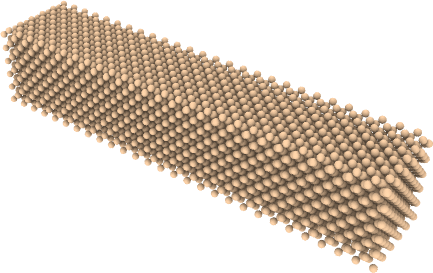
(a)	(b)

Figure 1: (a) Schematic illustration of the set-up for evaluating thermal conductivity of Si using NEMD. (b) Arrangement of Si atoms prior to the application of temperature gradient.

The set of inputs to LAMMPS is provided below in Table 1. Note that specific values for the length of the bar and the applied temperature gradient are not provided since we investigate thermal conductivity trends for a range of values of the two parameters as discussed later in Section 3. A careful analysis focused on minimizing temperature fluctuations during different stages of the simulation was performed to optimize for the choice of height and width of the bar as well as the duration of the simulation.

Lattice Constant, $a$ (Å)	5.43
Width, Height (Å)	22$a$
$\Delta t$ (ps)	0.0005
Simulation Run Length (ps)	320
Boundary Condition	Periodic
Lattice Structure	Diamond
Inter-atomic Potential	Stillinger-Weber

Table 1: Set of inputs for the NEMD simulation to estimate thermal conductivity in a Si bar using LAMMPS.

The NEMD simulation has three stages associated with it as illustrated below in the flow diagram. In the first stage, the NVT ensemble equilibrates the system to a specified bulk temperature, i.e., the temperature at which thermal conductivity is to be estimated. In the second stage, the NVE ensemble equilibrates the thermostats at their respective temperatures. It is followed by another NVE ensemble that captures the trajectory of individual atoms and results in a steady state estimate for the thermal energy exchange between the two thermostats.

NVT       $\rightarrow$       NVE       $\rightarrow$       NVE

[Equilibrate system to 300 K]    [Equilibrate thermostats]         [Generate Data]

N: Number of Atoms   V: Volume   T: Temperature   E: Energy

The steady state exchange energy ($q$) is used in Fourier’s law to estimate bulk thermal conductivity ($\kappa$) for the Si bar:

$$\kappa=\frac{q^{\prime\prime}}{\left|\frac{dT}{dz}\right|}$$ (1)

where $q^{\prime\prime}$ denotes the steady state heat flux (W/m²) and $\left|\frac{dT}{dz}\right|$ denotes the magnitude of the applied temperature gradient along the direction of heat flow (see Figure 1(a)).

3 Response Surface of the Discrepancy

As discussed earlier in Section 1, bulk thermal conductivity estimates using NEMD simulations are lower than measured values primarily due to reduction in mean free path associated with phonon transport. Additionally, the introduction of thermostats causes significant fluctuations in the applied temperature gradient, especially in their vicinity. We illustrate this phenomenon by plotting the temperature distribution along the length of the bar in Figure 2.

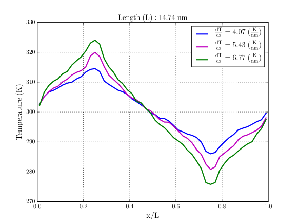
Figure 2: Temperature distribution along a Si bar of length 14.74 nm for different scenarios of applied temperature gradient.

In this section, we focus on the impact of system size, specifically the length of the Si bar as well as the applied temperature gradient on the discrepancy in bulk thermal conductivity between NEMD predictions and experimental data. For this purpose, we consider a range of values for the bar length and the temperature gradient. In order to determine the discrepancy trends, one might consider evaluating the thermal conductivity using NEMD simulations for a large set of values of length and temperature gradient. However, considering the computational expense associated with each pair of values, this approach quickly becomes computationally prohibitive. Instead, we construct a response surface using a 2D PC representation of the discrepancy which requires NEMD predictions for a small number of combinations of length and temperature gradient values as discussed in the following section.

3.1 Polynomial Chaos Response Surface

The PC response surface approximates the functional relationship between independent and uncertain inputs $(\bm{\theta})$ to a model with the output $\mathcal{Y}$. Essentially, it is a truncated expansion with polynomial basis functions that converges in a least-squares sense. For an accurate PC representation, the output should vary smoothly with respect to the uncertain inputs [24] and must be L-2 integrable:

$$\mathbb{E}[\mathcal{Y}^{2}]=\int_{\mathcal{D}_{\bm{\theta}}}\mathcal{Y}^{2}\mathbb{P}(\bm{\theta})d\bm{\theta}<\infty$$ (2)

where $\mathcal{D}_{\bm{\theta}}$ is the domain of the input parameter space and $\mathbb{P}(\bm{\theta})$ is the joint probability distribution of individual components of $\bm{\theta}$. In the present setting, $\bm{\theta}$: $\{L,\frac{dT}{dz}\}$ and the output, $\mathcal{Y}$ is the discrepancy ($\epsilon_{\mbox{\tiny{d}}}$ = $\lvert\kappa_{\mbox{\tiny{MD}}}$ - $\kappa_{\mbox{\tiny{E}}}\rvert$) in bulk thermal conductivity predictions from NEMD ($\kappa_{\mbox{\tiny{MD}}}$) and experimental data ($\kappa_{\mbox{\tiny{E}}}$), at a given temperature, $T$. The PC representation of $\epsilon_{\mbox{\tiny{d}}}$ is given as:

$$\epsilon_{\mbox{\tiny{d}}}\approx\mathcal{\epsilon}_{\mbox{\tiny{d}}}^{\mbox{\tiny{PCE}}}=\sum_{\bm{k}\in\mathcal{I}}c_{\bm{k}}(T)\Psi_{\bm{k}}(\bm{\xi(\theta)})$$ (3)

Individual components of the uncertain input vector, $\bm{\theta}$ are parameterized in terms of canonical random variables, $\bm{\xi}$ distributed uniformly in the interval $[-1,1]$. $\Psi_{\bm{k}}$’s are multivariate polynomial basis functions, orthonormal with respect to the joint probability distribution of $\bm{\xi}$. The degree of truncation in the above expansion is denoted by $\bm{k}$, a subset of the multi-index set $\mathcal{I}$ that comprises of individual degrees of univariate polynomials in $\Psi_{\bm{k}}$. The PC coefficients, $c_{\bm{k}}$’s can be estimated using either numerical quadrature or advanced techniques involving basis pursuit de-noising [25], compressive sampling [26], and least angle regression [27] suited for large-dimensional applications. However, in our case, since the response surface is 2D, we use Gauss-Legendre quadrature to obtain accurate estimates of the PC coefficients.

In order to construct the response surface of the discrepancy, we consider respective intervals for the Si bar length, $L$ and the applied temperature gradient, $\frac{dT}{dz}$ as $[50a,100a]$ (Å) and $[\frac{1.5}{a},\frac{2.5}{a}]$ ($\frac{\mbox{\tiny{K}}}{\tiny{\mbox{\AA}}}$); $a$ being the lattice constant. For the considered length interval, the number of atoms in the simulation were observed to range from 201344 to 379456. It must be noted that our focus is on illustrating a methodology for constructing a response surface that sufficiently captures the relationship between the inputs: $L$, $\frac{dT}{dz}$ and the discrepancy, $\epsilon_{d}$. Hence, we believe that the considered range for $L$ is large enough to be able to capture the input-output trends as presented further below, while ensuring reasonable computational effort. Additionally, the underlying noise associated with NEMD simulations was found to be negligible in the considered range for $\frac{dT}{dz}$ since we use average temperature at the bin point during the data production NVE ensemble.

NEMD predictions of $\kappa_{\text{MD}}$ are obtained at 25 Gauss-Legendre quadrature nodes (or points) in the 2D parameter space as highlighted in Figure 4(a) and 4(b). Note that 5 points are considered along $L$ and $\frac{dT}{dz}$ assuming that a fourth order polynomial basis would be sufficient in both cases, and the associated computational effort is not too large. Later, we assess the validity of our assumption by verifying the accuracy of the resulting response surface.

The discrepancy between $\kappa_{\mbox{\tiny{MD}}}$ and $\kappa_{\mbox{\tiny{E}}}$ is computed at the quadrature nodes as illustrated in Figure 3(a) to estimate the PC coefficients. The spectrum of resulting PC coefficients is illustrated in Figure 3(b). Note that the value of $\kappa_{\mbox{\tiny{E}}}$ is considered to be 149 W/m/K as provided in [12]. Response surfaces constructed at the bulk temperature, $T$ = 300 K and 500 K are illustrated in Figure 4(a) and 4(b) respectively.

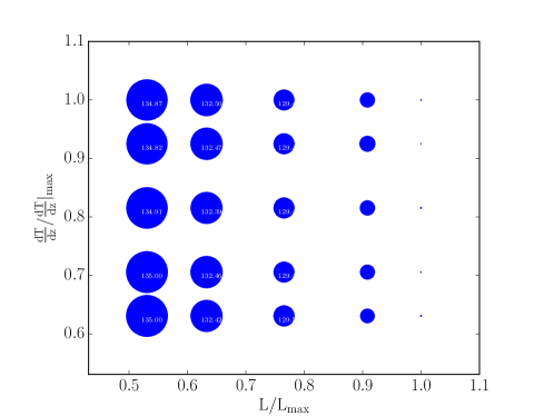
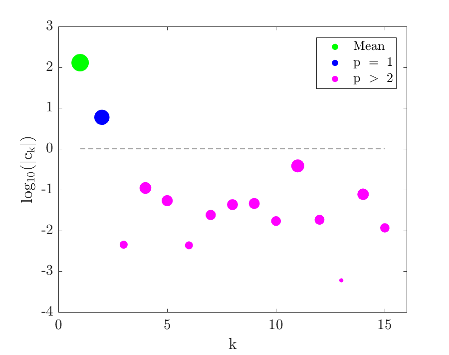
(a)	(b)

Figure 3: (a) Realizations of discrepancy in bulk thermal conductivity at the Gauss-Legendre quadrature notes are depicted using circles. The size of the circle in each case is proportional to the discrepancy estimate, also provided in cases where it is observed to be relatively large. (b) Spectrum of PC coefficients is depicted using circles of varying sizes, proportional to the log value of their magnitude. The above computations were performed at 300 K.

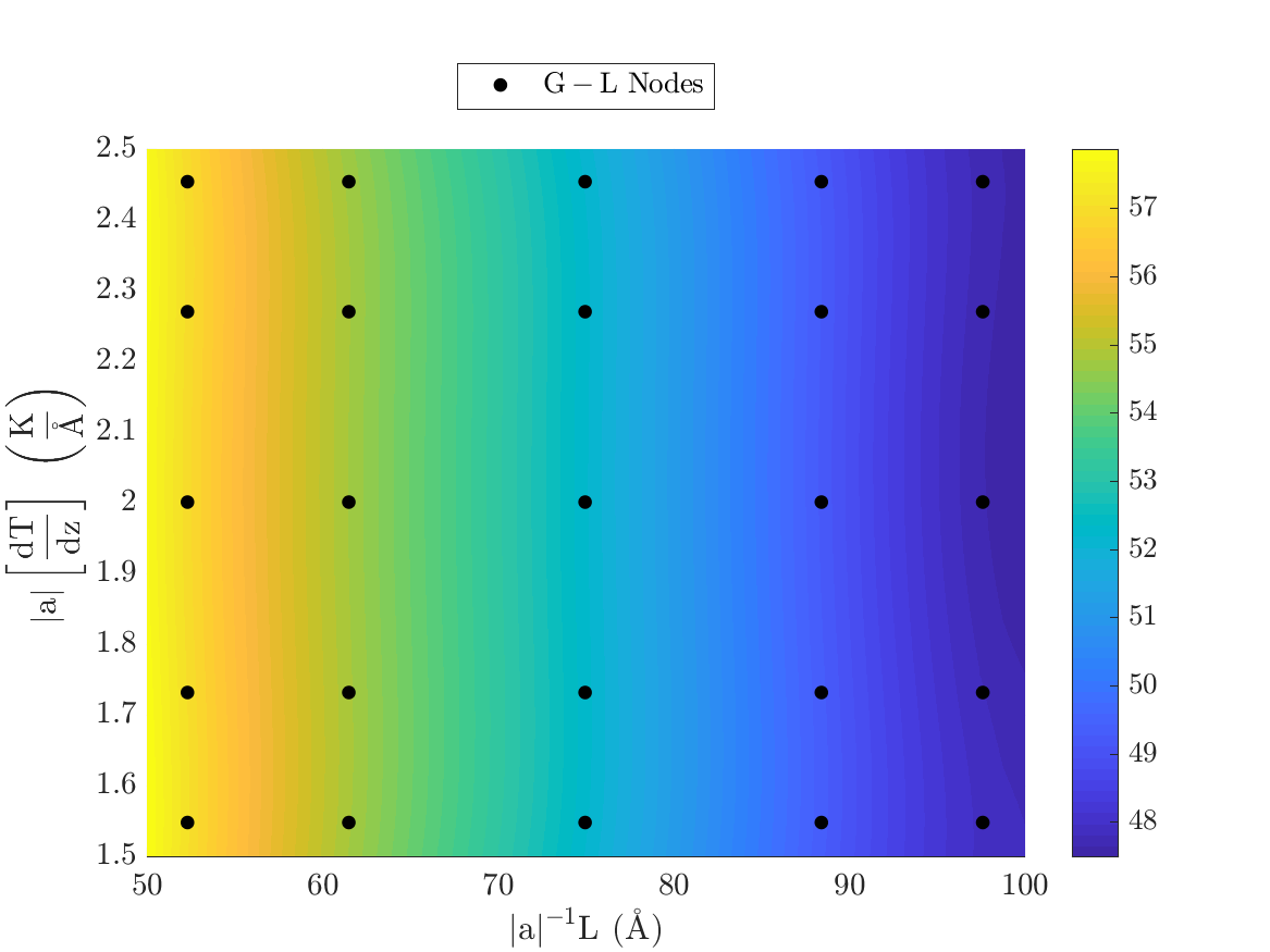
(a)	(b)

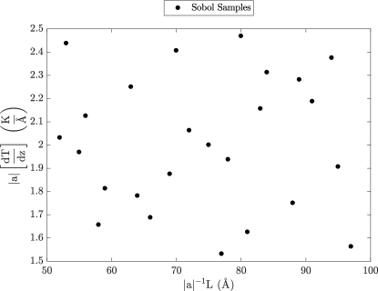
(c)

Figure 4: Response surface of the discrepancy in bulk thermal conductivity at (a) $T$ = 300 K and (b) $T$ = 500 K. Gauss-Legendre quadrature nodes are highlighted in both cases. (c) Sobol samples in the 2D domain used for verifying the accuracy of the response surfaces. Here, $|a|$ denotes the magnitude of the lattice constant.

As expected, the discrepancy is observed to decrease with the bar length ($L$) due to increase in the mean free path. It is however interesting to note that the variation in discrepancy due to changes in the applied temperature gradient in the considered range is found to be negligible. The accuracy of the response surface is verified by computing a relative L-2 norm of the error ($\varepsilon_{\tiny{\mbox{L-2}}}$) on an independent set of Sobol samples [28] (see Figure 4(c)) in the 2D parameter domain as follows:

$$\varepsilon_{\tiny{\mbox{L-2}}}=\frac{\left[\sum_{j}(\epsilon_{\tiny{\mbox{d},j}}^{\mbox{\tiny{MD}}}-\epsilon_{\tiny{\mbox{d},j}}^{\mbox{\tiny{PCE}}})^{2}\right]^{\frac{1}{2}}}{\left[\sum_{j}(\epsilon_{\tiny{\mbox{d},j}}^{\mbox{\tiny{MD}}})^{2}\right]^{\frac{1}{2}}}$$ (4)

A response surface was also constructed at $T$ = 1000 K (plot not included for brevity) and the impact of varying the temperature gradient on the discrepancy was still observed to be negligible. In all cases, $\varepsilon_{\tiny{\mbox{L-2}}}$ in Eq. 4 was estimated to be of $\mathcal{O}(10^{-3})$ thereby indicating that the response surfaces could be used to predict the discrepancy for a given point ($L$,$\frac{dT}{dz}$) in the considered domain with reasonable accuracy. As an additional verification step, we plot the inverse of thermal conductivity against the inverse of bar length using data from NEMD simulations as well as predictions from the response surface ($\kappa_{\mbox{\tiny{MD}}}~{}=~{}\kappa_{\mbox{\tiny{E}}}~{}-~{}\epsilon_{\mbox{\tiny{d}}}$) in Figure 5.

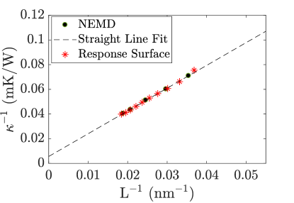
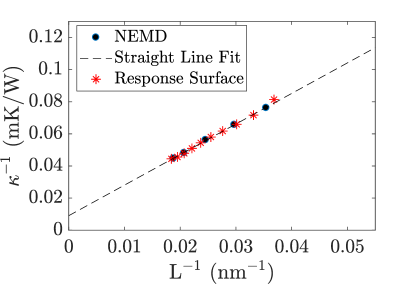
(a)	(b)

Figure 5: Inverse of the bulk thermal conductivity estimates are plotted against the inverse of Si bar length using predictions from NEMD as well as estimates from the response surface at (a) $T$ = 300 K and (b) $T$ = 500 K. A straight line fit to the estimates is also illustrated in each case.

It is observed that the response surface estimates exhibit an expected linear trend, consistent with NEMD predictions. Using the y-intercept of the straight line fit, the bulk thermal conductivity was estimated as 178.52 W/m/K and 110.64 W/m/K at 300 K and 500 K respectively. Using a wider range for system length would help improve these estimates. However, as discussed earlier, our focus is on demonstrating a methodology for quantifying the uncertainties (with limited resources) in bulk thermal conductivity predictions using NEMD as opposed to determining accurate estimates for the same. Constructing response surfaces using a relatively small number of NEMD predictions thus offers potential for huge computational savings for studies aimed at predicting thermal conductivity trends and quantifying the discrepancy with measurements for a wide range of system sizes, applied temperature gradients as well as bulk temperatures.

In the following sections, we shift our focus towards understanding the impact of the uncertainty in SW potential parameter values on the uncertainty in NEMD predictions for bulk thermal conductivity in Si.

4 Sensitivity Analysis of the Inter-atomic Potential

As discussed earlier in Section 1, bulk thermal conductivity estimates in NEMD are dependent on the choice of the inter-atomic potential as well as values associated with the individual potential parameters. In the case of silicon, the Stillinger-Weber (SW) is a commonly used inter-atomic potential (see [29, 30, 31, 32, 33] and references therein). Functional form of the SW potential is given as follows:

$$\Phi=\sum\limits_{i,j(i<j)}\phi_{2}(A,B,p,q,\alpha)\hskip 2.84526pt+\sum\limits_{i,j,k(i<j<k)}\phi_{3}(\lambda,\gamma)$$ (5)

where $\phi_{2}$ and $\phi_{3}$ represent two-body and three-body atomic interactions respectively [14].

Although the SW potential is used for a wide variety of Si systems, according to Stillinger and Weber, the set of nominal values as provided below in Table 2 were based on a constrained search in the 7D parameter space to ensure structural stability and agreement with the available experimental data [14].

$A$	$B$	$p$	$q$	$\alpha$	$\lambda$	$\gamma$
7.049556277	0.6022245584	4.0	0.0	1.80	21.0	1.20

Table 2: Nominal values of the parameters of the Stillinger-Weber inter-atomic potential [14].

It is noteworthy that the underlying analysis which led to these estimates of the nominal values did not account for the presence of uncertainty due to measurement error, noise inherent in MD predictions, inadequacies pertaining to the potential function, and parametric uncertainties. It is therefore likely that the proposed nominal estimates could be improved depending upon the application. Hence, it is critical to understand the effects of uncertainty in SW potential parameters on bulk thermal conductivity predictions using NEMD. For this purpose, a possible approach could involve a global sensitivity analysis of NEMD predictions on the SW potential parameters by estimating the so-called Sobol' indices [34]. However, obtaining converged estimates of Sobol' indices typically requires tens of thousands of model evaluations to be able to numerically approximate multi-dimensional integrals associated with the expectation and variance operators, especially in case $\bm{\theta}$, the vector of uncertain model inputs is high-dimensional:

$$\mathcal{T}_{i}=\frac{\mathbb{E}_{\bm{\theta}\sim i}[\mathbb{V}_{\theta_{i}}(\mathcal{G}|\bm{\theta}_{\sim i})]}{\mathbb{V}(\mathcal{G})}$$ (6)

where $\mathcal{T}_{i}$ is the Sobol' total-effect index, $\mathcal{G}$ denotes the model output, $\mathbb{E}_{\bm{\theta}\sim i}[]$ is an expectation over all but the $i^{\mbox{th}}$ component of $\bm{\theta}$, and $\mathbb{V}_{\theta_{i}}()$ is the variance taken over $\theta_{i}$. Li and Mahadevan recently proposed a computationally efficient method for estimating the first-order Sobol' index [35]. However, since NEMD is compute-intensive, estimating the Sobol' indices directly would be impractical in the present scenario. Hence, instead of estimating Sobol' sensitivity indices, we focus our attention on the upper bound of the Sobol' total-effect index to determine the relative importance of SW potential parameters. It is observed that for a given application, it might be possible to converge to the upper bound on Sobol' index with only a few iterations ($\mathcal{O}(10^{1})$) [36]. In that case, estimates of the upper bound could be used in lieu of the Sobol' indices to determine relative importance of the parameters and hence reduce the associated computational effort by several order of magnitude. The upper bound of the Sobol' total effect index ($\mathcal{T}_{i}$) can be expressed in terms of a derivative-based sensitivity measure (DGSM), $\mu_{i}$, the Poincaré constant ($\mathcal{C}_{i}$), and the total variance of the observed quantity ($V$) [37, 38] as follows:

$$\mathcal{T}_{i}\leq\frac{\mathcal{C}_{i}\mu_{i}}{V}~{}(\propto\hat{\mathcal{C}_{i}\mu_{i}})$$ (7)

The derivative-based sensitivity measure, $\mu_{i}$ for a given parameter, $\theta_{i}$ is defined as an expectation of the derivative of the output ($G(\bm{\theta})$) with respect to that parameter:

$$\mu_{i}=\mathbb{E}\left[\left(\frac{\partial G(\bm{\theta})}{\partial\theta_{i}}\right)^{2}\right]$$ (8)

Latin hypercube sampling in the 7D parameter space is used to estimate $\mu_{i}$. Note that $G$ must exhibit a smooth variation with each parameter so that the derivative in Eq. 8 can be estimated with reasonable accuracy, analytically or numerically. We define a normalized quantity, $\hat{\mathcal{C}_{i}\mu_{i}}$ to ensure that its summation over all parameters is 1:

$$\hat{\mathcal{C}_{i}\mu_{i}}=\frac{\mathcal{C}_{i}\mu_{i}}{\sum_{i}\mathcal{C}_{i}\mu_{i}}$$ (9)

The choice of $\mathcal{C}_{i}$ is specific to the marginal probability distribution of the uncertain model parameter, $\theta_{i}$. The underlying methodology for implementing DGSM to the present application involving thermal transport in bulk Si, and our key findings are discussed in the following section.

4.1 DGSM for SW potential parameters

We aim to compute the DGSM and hence the corresponding upper bound on the Sobol' total effect index ($\mathcal{T}_{i}$) for each parameter in the SW potential. For this purpose, we introduce small perturbations ($\mathcal{O}(10^{-5})n_{i}$; $n_{i}$ being the nominal value) to the nominal values associated with each parameter and estimate the partial derivatives in Eq. 8 using finite difference. Hence, in order to compute $\mu_{i}$ using $N$ points in the d-dimensional parameter space, we require $N(d+1)$ model realizations. The SW potential parameters are considered to be uniformly distributed in a small interval around the nominal value in which case $\mathcal{C}_{i}$ is given as $(u-l)^{2}/\pi^{2}$ [38]; $u$ and $l$ being the upper and lower bounds of the interval respectively.

Performing NEMD simulations using perturbed values of the SW potential parameters could however be challenging. For certain combinations of the SW potential parameter values, the steady-state thermal energy exchange between the thermostats was found to be non-physical at the end of the simulation. We believe that this was observed in situations where the structure had deviated too far from the equilibrium state, and therefore the structural integrity of the bar was lost as illustrated in Figure 6(a).

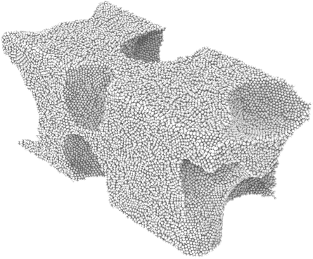
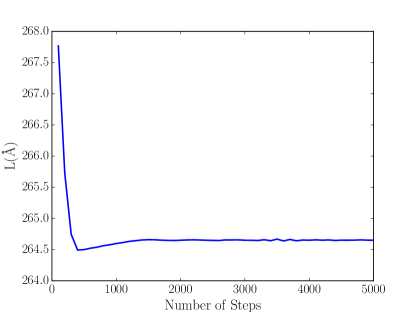
(a)	(b)

Figure 6: (a) A snapshot of the arrangement of atoms illustrating loss of structural integrity of the Si bar. (b) Si bar length is plotted against the number of time steps during the NPT ensemble stage of the simulation.

To avoid this issue, we added an NPT ensemble prior to NVT in the NEMD simulation as shown in the following diagram:

NPT       $\rightarrow$       NVT       $\rightarrow$       NVE       $\rightarrow$       NVE

[Relax the system] [Equilibrate system to 300 K]    [Equilibrate thermostats]         [Generate Data]

N: Number of Atoms   P: Pressure   V: Volume   T: Temperature   E: Energy

The NPT stage of the simulation was allowed to continue for a sufficiently long duration to ensure that the system is relaxed to a steady value of the bar length as shown in Figure 6(b).

The following algorithm provides the sequence of steps that were used to obtain approximate estimates of the sensitivity measures for the SW potential parameters. Note that the algorithm has been adapted to the specific application in this work. A generalized methodology with a more detailed discussion and its application to different class of problems will be presented in [39].

  Algorithm 1 Estimating parameter ranks using DGSM.

 

1:procedure DGSM

2:     Generate $n_{1}$ points in $\mathbb{R}^{d}$.$\triangleright$ $d$: Number of parameters i.e. 7 in this case

3:     Perturb each point along the $d$ directions to obtain a set of $n_{1}(d+1)$ points.

4:     Compute $\mu_{i}$ using model evaluations at the $n_{1}(d+1)$ points in Eq. 8

5:     Determine initial ranks, $\mathcal{R}^{old}$ based on $\hat{\mathcal{C}_{i}\mu_{i}}$ values for $\theta_{i}$.

6:     set $k$ = 1$\triangleright$ Iteration counter

7:     do

8:         Generate $n_{k}$ new points in $\mathbb{R}^{d}$.

9:         Perturb each point along the $d$ directions to obtain a set of $n_{k}(d+1)$ points.

10:         Compute and store model evaluations at the $n_{k}(d+1)$ points.

11:         Compute $\mu_{i}$ using prior model evaluations at $(d+1)(n_{1}+\sum_{j}^{k}n_{j})$ points.

12:         Determine new ranks, $\mathcal{R}^{new}$ based on updated $\hat{\mathcal{C}_{i}\mu_{i}}$ values.

13:         Compute $max\_pdev$ = max$\left(\frac{|\mu_{i,k}-\mu_{i,k-1}|}{\mu_{i,k-1}}\right)$.$\triangleright$ $max\_pdev$: Maximum percentage deviation in $\mu_{i}$ between successive iterations.

14:         set $k$ = $k$ + 1

15:     while ($\mathcal{R}^{\tiny{new}}$ $\neq$ $\mathcal{R}^{\tiny{old}}$ or $max\_pdev$ $>~{}\tau$)$\triangleright$ $\tau$: Tolerance

16:end procedure

 

For the present application, we begin with $n_{1}$ = 10 samples in the 7D parameter space and add 5 points at each iteration. Using a tolerance, $\tau$ = 0.05, the above algorithm took 4 iterations i.e. 25 points to provide approximate estimates for $\mu_{i}$. Since finite difference was used to estimate the derivatives in Eq. 8, it required 25(7+1) i.e. 200 MD runs. It must be noted that although the computational effort pertaining to the estimation of DGSM can be substantial, it is nevertheless several orders of magnitude smaller than directly estimating the Sobol' indices as mentioned earlier. In Figure 7, we plot $\hat{\mathcal{C}_{i}\mu_{i}}$ as obtained for the SW parameters at the end of 4 iterations. It appears that $\gamma$ is significantly more important than other parameters, whereas NEMD predictions are relatively less sensitive to $B$ and $p$. Large sensitivity towards $\gamma$ and $\alpha$ (cut-off radius) is in fact expected since these two parameters impact the lattice constant and hence the mean free path associated with the bulk thermal conductivity directly.

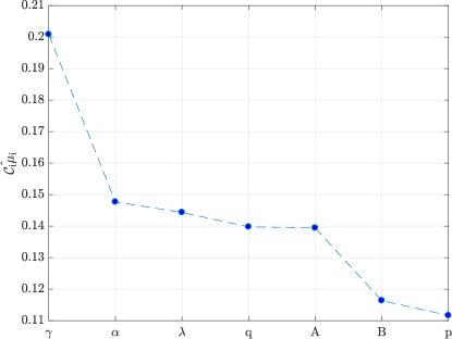
Figure 7: The quantity $\hat{\mathcal{C}_{i}\mu_{i}}$ as computed after 4 iterations and data at 200 points is plotted for each SW potential parameter.

In the following section, we exploit these observations based on DGSM to construct a reduced order surrogate. The surrogate enables forward propagation of uncertainty in the SW potential to the bulk thermal conductivity estimates, and the estimation of Sobol' sensitivity indices with minimal computational effort.

5 Reduced-order Surrogate

In this section, we focus our attention on constructing a surrogate that captures the dependence of uncertainty in NEMD predictions of the bulk thermal conductivity ($\kappa$) on input uncertainty in the SW potential parameters. The surrogate is a powerful tool that greatly minimizes the computational effort required for forward propagation of the uncertainty from input parameters to the output, Sobol' sensitivity analysis, and Bayesian calibration of the uncertain model parameters. Once again, we use polynomial chaos (used to construct response surfaces for discrepancy in Section 3) to construct the surrogate of the following functional form:

$$\kappa=\sum\limits_{\bm{s}\in\mathcal{A}}c_{\bm{s}}(T)\Psi_{\bm{s}}(\bm{\xi})$$ (10)

As discussed earlier in Section 3, several strategies are available to estimate the PC coefficients, $c_{\bm{s}}$. However, since the polynomial basis functions ($\Psi_{\bm{s}}(\bm{\xi}$)) are relatively high dimensional, we use a computationally efficient approach proposed by Blatman and Sudret to construct a PCE with sparse basis($\mathcal{A}$) using the LAR algorithm [27]. Furthermore, since the NEMD simulations are compute-intensive, estimating the PC coefficients in the 7D parameter space would still require a large amount of computational resources. Hence, we explore the possibility of reducing the dimensionality of the surrogate. For this purpose, we exploit our observations in Figure 7 where a significant jump in the $\hat{\mathcal{C}_{i}\mu_{i}}$ estimate is seen from $A$ to $B$ and thereby construct the PC surrogate in a 5D parameter space by fixing $B$ and $p$ at their nominal values. In the above equation, $\bm{\xi}:~{}\{\xi_{1}(A),\xi_{2}(q),\xi_{3}(\alpha),\xi_{4}(\lambda),\xi_{5}(\gamma)\}$ is a set of five canonical random variables, $\xi_{i}$ distributed uniformly in the interval [-1,1]. Prior intervals for the uncertain SW parameters are considered to be $\pm~{}10\%$ of their respective nominal estimates except for $q$ in which case it is [0,0.1]. In Figure 8, we plot the leave-one-out cross-validation error ($\epsilon_{\tiny{\mbox{LOO}}}$) [40], defined below in Eq. 11, against the number of model realizations used to construct the 5D PC surrogate. The software, UQLab [41] was used for estimating $\epsilon_{\tiny{\mbox{LOO}}}$ and constructing the surrogate. The leave-one-out cross validation error ($\epsilon_{\tiny{\mbox{LOO}}}$) is computed as:

$$\epsilon_{\tiny{\mbox{LOO}}}=\frac{\sum\limits_{i=1}^{N}\left(\mathcal{M}(\bm{x}^{(i)})-\mathcal{M}^{PCE\setminus i}(\bm{x}^{(i)})\right)^{2}}{\sum\limits_{i=1}^{N}\left(\mathcal{M}(\bm{x}^{(i)})-\hat{\mu}_{Y}\right)^{2}}$$ (11)

where $N$ denotes the number of realizations, $\mathcal{M}(\bm{x}^{(i)})$ is the model realization and $\mathcal{M}^{PCE\setminus i}(\bm{x}^{(i)})$ is the corresponding PCE estimate at $\bm{x}^{(i)}$. Note that the PCE is constructed using all points except $\bm{x}^{(i)}$. The quantity, $\hat{\mu}_{Y}$ = $\frac{1}{N}\sum\limits_{i=1}^{N}\mathcal{M}(\bm{x}^{(i)})$ is the sample mean of the realizations.

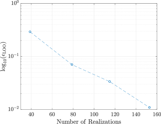
Figure 8: A convergence study for the 5D PCE wherein the leave-one-out error, $\epsilon_{\tiny{\mbox{LOO}}}$ is plotted against the number of realizations or NEMD runs used to estimate the PC coefficients.

It is found that in order for the PCE to converge to an accuracy of $\mathcal{O}(10^{-2})$ with respect to $\epsilon_{\tiny{\mbox{LOO}}}$, we require approximately 160 NEMD runs. In the following section, we focus on verifying the accuracy of the 5D PCE against the set of available NEMD predictions in the original 7D parameter space.

5.1 PC Surrogate Verification

The accuracy of the 5D PC surrogate is verified using two different strategies. The first strategy involves computing the relative L-2 norm of the difference between the available NEMD predictions (used earlier to estimate DGSM in Section 4) and estimates using the 5D surrogate as follows:

$$\epsilon_{\mbox{\tiny{L-2}}}=\frac{\left[\sum\limits_{i=1}^{N=25}\left(\mathcal{M}(\bm{\theta}_{\mbox{\tiny{7D}}}^{(i)})-\mathcal{M}^{PCE}(\bm{\theta}_{\mbox{\tiny{5D}}}^{(i)})\right)^{2}\right]^{\frac{1}{2}}}{\left[\sum_{i=1}^{N}\left(\mathcal{M}(\bm{\theta}_{\mbox{\tiny{7D}}}^{(i)})\right)^{2}\right]^{\frac{1}{2}}}\approx 6.88\times 10^{-2}$$ (12)

where $\mathcal{M}(\bm{\theta}_{\mbox{\tiny{7D}}}^{(i)})$ is the NEMD prediction in the original 7D parameter space, and $\mathcal{M}^{PCE}(\bm{\theta}_{\mbox{\tiny{5D}}}^{(i)})$ is the corresponding estimate using the reduced order surrogate (5D). Since $\epsilon_{\mbox{\tiny{L-2}}}$ is found to be $\mathcal{O}(10^{-2})$, the 5D surrogate can be considered as reasonably accurate from the perspective of relative L-2 error norm.

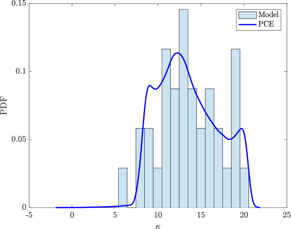
Figure 9: Comparison of bulk thermal conductivity ($\kappa$) distribution of Si based on a histogram plot using NEMD predictions (Model) at 25 points in the 7D parameter space and a probability distribution obtained using kernel density estimation of reduced-order surrogate estimates of $\kappa$ for 10⁶ samples in the 5D parameter space.

In the second strategy, we compare NEMD predictions and estimates from the 5D surrogate in a probabilistic sense. As shown in Figure 9, a histogram plot based on the available set of NEMD predictions for bulk thermal conductivity in the 7D parameter space is compared with its probability distribution, obtained using the reduced order surrogate and 10⁶ samples in the 5D parameter space described by the SW potential parameters: $\{A,q,\alpha,\lambda,\gamma\}$. It is observed that the probability density function (PDF) based on estimates from the reduced-order surrogate compares favorably with the histogram. Specifically, the corresponding mode values for $\kappa$ from the two plots are in close agreement, and the PDF reasonably captures the peaks as well as the spread in the bulk thermal conductivity distribution as observed in the histogram. Hence, the reduced-order surrogate is verified for accuracy in both cases.

As mentioned earlier, a PC surrogate can be used to estimate the Sobol' global sensitivity indices in a straightforward manner [42]. The Sobol' first order and total effect sensitivity indices estimated using the reduced-order surrogate and $10^{6}$ samples in the 5D parameter space are plotted using bar-graphs in Figure 10.

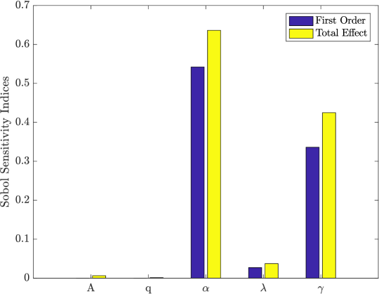
Figure 10: Sobol' first-order and total effect sensitivity indices of the SW potential parameters w.r.t the bulk thermal conductivity as obtained using the reduced order PC surrogate and 10⁶ samples in the 5D parameter space.

It is found that $\kappa$ is predominantly sensitive towards the choice of $\alpha$ and $\gamma$. This observation is consistent with our initial findings based on DGSM using 25 samples in the 7D parameter space. However, the DGSM estimate for $\gamma$ was found to be the highest in that case. While sensitivity towards $A$, $q$, and $\lambda$ is observed to be comparatively less in both cases, the Sobol' indices for the three parameters are estimated to be smaller by an order of magnitude compared to those for $\alpha$ and $\gamma$. Large quantitative disagreement in parametric sensitivity between DGSM and the Sobol' indices is however not unexpected essentially because the two metrics differ by construction. The former is based on an expectation of partial derivatives while the later is based on variance. Nevertheless, significant qualitative agreement pertaining to parameter importance in the two approaches is quite encouraging. Moreover, verification of the reduced-order surrogate for accuracy increases our confidence in implementing DGSM to ascertain the relative importance of the SW potential parameters and hence perform uncertainty analysis for the present application with minimal computational effort.

6 Bayesian Calibration

As discussed earlier in Section 1, the underlying methodology for determining the nominal estimates for SW potential parameters did not account for measurement error, inadequate functional form of the potential, inherent noise in MD predictions, and parametric uncertainties. Hence, there is a possibility of improving the estimates since using the same set of values for a wide variety of systems and applications is not ideal. A robust approach to calibrating the parameters in the presence of such uncertainties is made possible by using a Bayesian framework. The methodology aims at evaluating the so-called joint posterior probability distribution (referred to as the ‘posterior’) of the uncertain model parameters to be calibrated, using Bayes’ rule:

$$\mathcal{P}(\bm{X}|\bm{Y})\propto\mathcal{P}(\bm{Y}|\bm{X})\mathcal{P}(\bm{X})$$ (13)

where $\bm{X}$ is the set of uncertain model parameters, and $\bm{Y}$ is the available set of experimental data i.e. bulk thermal conductivity at different temperatures in the present case. We exploit our findings based on sensitivity analysis in Figure 10 and focus on calibrating $\alpha$ and $\gamma$ i.e. $\bm{X}:\{\alpha,\gamma\}$. $\mathcal{P}(\bm{X}|\bm{Y})$ is regarded as the posterior, $\mathcal{P}(\bm{Y}|\bm{X})$ is the ‘likelihood’, and $\mathcal{P}(\bm{X})$ is the joint prior probability distribution (referred to as the ‘prior’) of $\bm{X}$. The likelihood accounts for measurement error, and the discrepancy between experiments and model predictions, whereas, the prior is an initial guess for the distribution of uncertain model parameters in an interval. It also accounts for the availability of the expert opinion pertaining to their estimates. The posterior provides an estimate of the most likely value of the uncertain model parameters based on prior uncertainty, experimental data used for calibration and the associated measurement error, and model discrepancy. Additionally, the posterior is often used to quantify the uncertainty associated with model predictions. Several algorithms based on the Markov chain Monte Carlo (MCMC) technique are available for sampling the posterior [43, 44, 45].

Evaluating the joint posterior of $\alpha$ and $\gamma$ using MCMC typically requires a large amount of computational effort and is not the focus of this work. Instead, we compute and plot the joint likelihood on a 2D cartesian grid described by $\alpha$ and $\gamma$ using Eq. 14 as illustrated in Figure 11(a). For this purpose, we consider the priors of $\alpha$ and $\gamma$ to be independent and uniformly distributed in the intervals, [1.62,1.98] and [1.08,1.32] respectively. Consequently, the posterior is proportional to the likelihood, considered to be a Gaussian:

$$\mathcal{P}(\bm{Y}|\bm{X})=\frac{1}{\sqrt{2\pi\sigma^{2}}}\exp\left[-\frac{(\kappa_{\tiny{\mbox{E}}}-\kappa_{\tiny{\mbox{MD}}})^{2}}{2\sigma^{2}}\right]$$ (14)

where $\sigma$ is the standard deviation of the measurement error, and $(\kappa_{\tiny{\mbox{E}}}-\kappa_{\tiny{\mbox{MD}}})$ is the discrepancy between NEMD predictions ($\kappa_{\tiny{\mbox{MD}}}$) and experimental data ($\kappa_{\tiny{\mbox{E}}}$). Experimental data for $\kappa_{\tiny{\mbox{E}}}$ at 300 K (149 W/m/K [12]) is used to compute the joint likelihood. It must be noted that the likelihood function in Eq. 14 could be refined further by accounting for a model discrepancy term and hence calibrating the associated parameters in addition to the uncertain model inputs [46, 47].

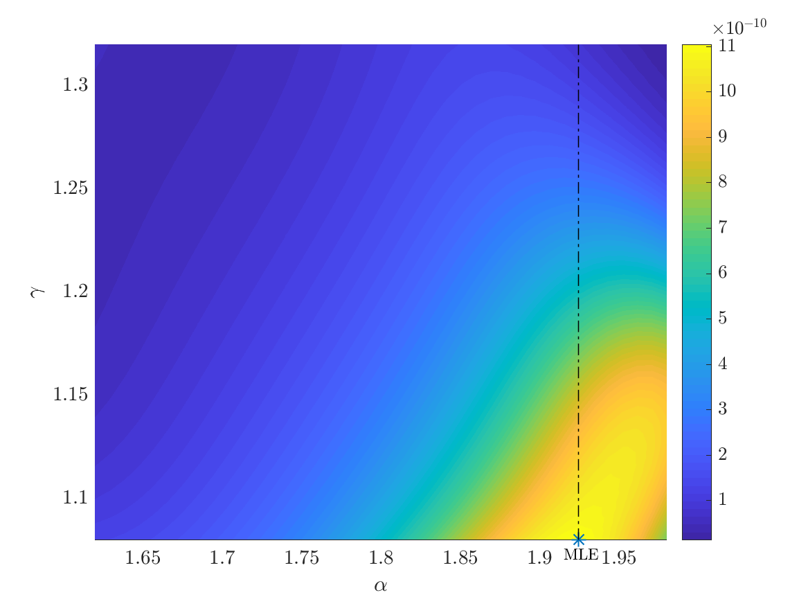
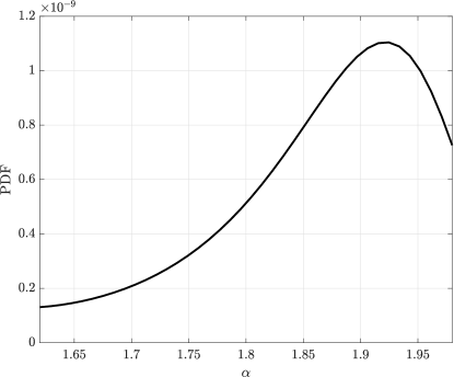
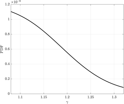
(a) (b) (c)

Figure 11: (a) The joint likelihood of ($\alpha$,$\gamma$) as estimated using Eq. 14 is plotted on a 2D cartesian grid. The maximum likelihood estimate (MLE) is also highlighted. Marginal likelihoods for $\alpha$ and $\gamma$ are plotted in (b) and (c) respectively.

Marginal distributions for $\alpha$ and $\gamma$ are shown in Figure 11(b) and Figure 11(c) respectively. As mentioned above, the joint likelihood plot is based on the bulk thermal conductivity measurement at 300 K. An enhanced set of experimental measurements at different bulk temperatures would help improve the accuracy of the calibration process considering the measurement noise is not too large. Moreover, it would help capture the correlation between calibration parameters across temperatures at which the data is available. However, a reduced-order surrogate would be needed at each temperature in order to make the MCMC tractable.

7 Summary and Discussion

In this paper, we have attempted to identify and address some of the challenges pertaining to uncertainty quantification of bulk thermal conductivity predictions using non-equilibrium molecular dynamics (NEMD) simulations. Specifically, we focused on investigating the impact of system size, and fluctuations in the applied thermal gradient on predictions. In order to quantify the discrepancy between NEMD predictions and experiments, response surfaces were constructed at bulk temperatures, $T$ = 300 K, 500 K, and 1000 K. It was found that the discrepancy is predominantly impacted by size while the effect of fluctuations in the applied thermal gradient is negligible in the considered interval. The response surface approach presented here relies on a small number of MD runs and enables an accurate estimation of discrepancy at a given temperature and a point in the 2D parameter space described by system-size and the applied thermal gradient.

A possible enhancement of nominal SW parameter estimates for a given application and the choice of material system is also highlighted in this work. To enable this, we focus our efforts on understanding the sensitivity of predictions on individual potential parameters. In order to reduce the computational effort, we estimate the derivative-based sensitivity measures (DGSM) and hence the upper bound on Sobol' total-effect sensitivity index using random samples in the 7D parameter space. While individual measures for the 7 parameters are not too distant from each other, the predictions seem to be most sensitive towards $\gamma$. Sensitivity measures for $\alpha$, $\lambda$, $q$, and $A$ are found to be comparable while those for $B$ and $p$ are relatively small.

A polynomial chaos surrogate model for the bulk thermal conductivity (observable) as a function of SW potential parameters at the bulk temperature of 300 K is constructed. The surrogate helps reduce the computational effort required for forward propagation of the uncertainty from parameters to the observable as well as for estimating the Sobol' sensitivity indices. Furthermore, the surrogate could be used to accelerate parameter calibration in a Bayesian setting. However, since the surrogate relies on NEMD predictions, the underlying computational effort is nevertheless significantly large. To circumvent this challenge, we exploit our initial findings based on DGSM and construct a reduced-order surrogate in 5 dimensions by fixing the parameters, $B$ and $p$. We verify its accuracy by estimating the relative L-2 norm of the error between NEMD predictions in the full space and the reduced-order surrogate predictions, and by comparing the probability density of the bulk thermal conductivity in Figure 9. Furthermore, our initial sensitivity trends based on DGSM-analysis using 25 samples seem to agree favorably with Sobol' sensitivity analysis based on 10⁶ samples. Hence, it can be said that DGSM-based analysis with a few samples could offer huge computational gains by reliably reducing the dimensionality of a surrogate for uncertainty analysis.

Finally, we highlight key aspects of parameter calibration in a Bayesian setting. The underlying motivation stems from the fact that the nominal estimates of the SW parameters did not consider measurement error, simulation noise, model form error, and parametric uncertainties. Calibration in a Bayesian framework allows us to incorporate such errors and uncertainties in an efficient manner and provides a joint posterior distribution of the uncertain parameters. To minimize computational costs pertaining to the calibration process, we suggest the following sequence of steps: First, perform DGSM analysis to identify parameters that are not so important. Second, construct a reduced-order surrogate based on DGSM-analysis and verify its accuracy. Third, compute the Sobol' sensitivity indices using the surrogate to identify parameters for calibration. Fourth, construct a second surrogate in the reduced subspace described by the calibration parameters, and quantify the surrogate error to be accounted for in calibration. Fifth, evaluate the joint posterior using an efficient MCMC-based algorithm such as adaptive Metropolis [43] and its variants [44, 48].

It is important to note that the strategies presented in this work are not restricted to a Si bar and the Stillinger-Weber potential, and could be extended to a wide range of applications and inter-atomic potentials for the purpose of uncertainty quantification.

References

- [1] T. Dumitrica. Trends in Computational Nanomechanics: Transcending Length and Time Scales, volume 9. Springer Science & Business Media, 2010.
- [2] P.K. Schelling, S.R. Phillpot, and P. Keblinski. Comparison of atomic-level simulation methods for computing thermal conductivity. Physical Review B, 65(14):144306, 2002.
- [3] J.E. Turney, E.S. Landry, A.J.H. McGaughey, and C.H. Amon. Predicting phonon properties and thermal conductivity from anharmonic lattice dynamics calculations and molecular dynamics simulations. Physical Review B, 79(6):064301, 2009.
- [4] X. W. Zhou, S. Aubry, R. E. Jones, A. Greenstein, and P. K. Schelling. Towards more accurate molecular dynamics calculation of thermal conductivity: Case study of gan bulk crystals. Phys. Rev. B, 79:115201, Mar 2009.
- [5] E.S. Landry and A.J.H. McGaughey. Thermal boundary resistance predictions from molecular dynamics simulations and theoretical calculations. Physical Review B, 80(16):165304, 2009.
- [6] A.J.H. McGaughey and M. Kaviany. Phonon transport in molecular dynamics simulations: Formulation and thermal conductivity prediction. Advances in Heat Transfer, 39:169–255, 2006.
- [7] B. Ni, T. Watanabe, and S.R. Phillpot. Thermal transport in polyethylene and at polyethylene–diamond interfaces investigated using molecular dynamics simulation. Journal of Physics: Condensed Matter, 21(8):084219, 2009.
- [8] L. Shi, D. Yao, G. Zhang, and B. Li. Size dependent thermoelectric properties of silicon nanowires. Applied Physics Letters, 95(6):063102, 2009.
- [9] S.-C. Wang, X.-G. Liang, X.-H. Xu, and T. Ohara. Thermal conductivity of silicon nanowire by nonequilibrium molecular dynamics simulations. Journal of Applied Physics, 105(1):014316, 2009.
- [10] N. Papanikolaou. Lattice thermal conductivity of sic nanowires. Journal of Physics: Condensed Matter, 20(13):135201, 2008.
- [11] W.M. Haynes. CRC handbook of chemistry and physics. CRC press, 2014.
- [12] H.R. Shanks, P.D. Maycock, P.H. Sidles, and G.C. Danielson. Thermal conductivity of silicon from 300 to 1400 k. Physical Review, 130(5):1743, 1963.
- [13] W. Evans, R. Prasher, J. Fish, P. Meakin, P. Phelan, and P. Keblinski. Effect of aggregation and interfacial thermal resistance on thermal conductivity of nanocomposites and colloidal nanofluids. International Journal of Heat and Mass Transfer, 51(5-6):1431–1438, 2008.
- [14] F.H. Stillinger and T.A. Weber. Computer simulation of local order in condensed phases of silicon. Physical review B, 31(8):5262, 1985.
- [15] Z. Wang, S. Safarkhani, G. Lin, and X. Ruan. Uncertainty quantification of thermal conductivities from equilibrium molecular dynamics simulations. International Journal of Heat and Mass Transfer, 112:267–278, 2017.
- [16] F. Rizzi, H.N. Najm, B.J. Debusschere, K. Sargsyan, M. Salloum, H. Adalsteinsson, and O.M. Knio. Uncertainty quantification in md simulations. part i: Forward propagation. Multiscale Modeling & Simulation, 10(4):1428–1459, 2012.
- [17] P. Marepalli, J.Y. Murthy, B. Qiu, and X. Ruan. Quantifying uncertainty in multiscale heat conduction calculations. Journal of Heat Transfer, 136(11):111301, 2014.
- [18] L.C. Jacobson, R.M. Kirby, and V. Molinero. How short is too short for the interactions of a water potential? exploring the parameter space of a coarse-grained water model using uncertainty quantification. The Journal of Physical Chemistry B, 118(28):8190–8202, 2014.
- [19] D. Xiu and G.E. Karniadakis. The wiener–askey polynomial chaos for stochastic differential equations. SIAM journal on scientific computing, 24(2):619–644, 2002.
- [20] R. Ghanem and P.D. Spanos. Polynomial chaos in stochastic finite elements. Journal of Applied Mechanics, 57(1):197–202, 1990.
- [21] O. Le Maître and O.M. Knio. Spectral methods for uncertainty quantification: with applications to computational fluid dynamics. Springer Science & Business Media, 2010.
- [22] I.M. Sobol and S. Kucherenko. Derivative based global sensitivity measures. Procedia-Social and Behavioral Sciences, 2(6):7745–7746, 2010.
- [23] S. Plimpton, P. Crozier, and A. Thompson. Lammps-large-scale atomic/molecular massively parallel simulator. Sandia National Laboratories, 18:43–43, 2007.
- [24] M. Vohra, J. Winokur, K.R. Overdeep, P. Marcello, T.P. Weihs, and O.M. Knio. Development of a reduced model of formation reactions in zr-al nanolaminates. Journal of Applied Physics, 116(23):233501, 2014.
- [25] J. Peng, J. Hampton, and A. Doostan. A weighted l1-minimization approach for sparse polynomial chaos expansions. Journal of Computational Physics, 267:92–111, 2014.
- [26] J. Hampton and A. Doostan. Compressive sampling of polynomial chaos expansions: Convergence analysis and sampling strategies. Journal of Computational Physics, 280:363–386, 2015.
- [27] G. Blatman and B. Sudret. Adaptive sparse polynomial chaos expansion based on least angle regression. Journal of Computational Physics, 230(6):2345–2367, 2011.
- [28] A. Saltelli, P. Annoni, I. Azzini, F. Campolongo, M. Ratto, and S. Tarantola. Variance based sensitivity analysis of model output. design and estimator for the total sensitivity index. Computer Physics Communications, 181(2):259–270, 2010.
- [29] M. Laradji, D.P. Landau, and B. Dünweg. Structural properties of Si 1- x Ge x alloys: A monte carlo simulation with the stillinger-weber potential. Physical Review B, 51(8):4894, 1995.
- [30] X. Zhang, H. Xie, M. Hu, H. Bao, S. Yue, G. Qin, and G. Su. Thermal conductivity of silicene calculated using an optimized stillinger-weber potential. Physical Review B, 89(5):054310, 2014.
- [31] J.-W. Jiang. Parametrization of stillinger–weber potential based on valence force field model: application to single-layer MoS2 and black phosphorus. Nanotechnology, 26(31):315706, 2015.
- [32] T. Watanabe and I. Ohdomari. Modeling of SiO2/Si (100) interface structure by using extended-stillinger-weber potential. Thin Solid Films, 343:370–373, 1999.
- [33] X.W. Zhou, D.K. Ward, J.E. Martin, F.B. Van Swol, J.L. Cruz-Campa, and D. Zubia. Stillinger-weber potential for the ii-vi elements Zn-Cd-Hg-S-Se-Te. Physical Review B, 88(8):085309, 2013.
- [34] I.M. Sobol. Global sensitivity indices for nonlinear mathematical models and their monte carlo estimates. Mathematics and computers in simulation, 55(1-3):271–280, 2001.
- [35] C. Li and S. Mahadevan. An efficient modularized sample-based method to estimate the first-order Sobol index. Reliability Engineering & System Safety, 153:110–121, 2016.
- [36] S. Kucherenko and B. Iooss. Derivative-based global sensitivity measures. Handbook of Uncertainty Quantification, pages 1–24, 2016.
- [37] M. Lamboni, B. Iooss, A.-L. Popelin, and F. Gamboa. Derivative-based global sensitivity measures: general links with Sobol indices and numerical tests. Mathematics and Computers in Simulation, 87:45–54, 2013.
- [38] O. Roustant, J. Fruth, B. Iooss, and S. Kuhnt. Crossed-derivative based sensitivity measures for interaction screening. Mathematics and Computers in Simulation, 105:105–118, 2014.
- [39] M. Vohra, A. Alexanderian, C. Safta, and S. Mahadevan. Sensitivity-driven adaptive construction of reduced-space surrogates. arXiv preprint arXiv:1806.06285, 2018.
- [40] G. Blatman and B. Sudret. An adaptive algorithm to build up sparse polynomial chaos expansions for stochastic finite element analysis. Probabilistic Engineering Mechanics, 25(2):183–197, 2010.
- [41] S. Marelli and B. Sudret. UQLab: A framework for uncertainty quantification in matlab. In Vulnerability, Uncertainty, and Risk: Quantification, Mitigation, and Management, pages 2554–2563. 2014.
- [42] B. Sudret. Global sensitivity analysis using polynomial chaos expansions. Reliability Engineering & System Safety, 93(7):964–979, 2008.
- [43] H. Haario, E. Saksman, J. Tamminen, et al. An adaptive Metropolis algorithm. Bernoulli, 7(2):223–242, 2001.
- [44] H. Haario, M. Laine, A. Mira, and E. Saksman. Dram: efficient adaptive MCMC. Statistics and Computing, 16(4):339–354, 2006.
- [45] M. Xu, B. Lakshminarayanan, Yee W. Teh, J. Zhu, and B. Zhang. Distributed bayesian posterior sampling via moment sharing. In Advances in Neural Information Processing Systems, pages 3356–3364, 2014.
- [46] M.C. Kennedy and A. O’Hagan. Bayesian calibration of computer models. Journal of the Royal Statistical Society: Series B (Statistical Methodology), 63(3):425–464, 2001.
- [47] Y. Ling, J. Mullins, and S. Mahadevan. Selection of model discrepancy priors in bayesian calibration. Journal of Computational Physics, 276:665–680, 2014.
- [48] P.J. Green and A. Mira. Delayed rejection in reversible jump metropolis–hastings. Biometrika, 88(4):1035–1053, 2001.