X-ray short-time lags in the Fe-K energy band produced by scattering clouds in active galactic nuclei

Abstract

X-rays illuminating the accretion disc in active galactic nuclei give rise to an iron K line and its associated reflection spectrum which are lagged behind the continuum variability by the light-travel time from the source to the disc. The measured lag timescales in the iron band can be as short as $\sim R_{g}/c$, where $R_{g}$ is the gravitational radius, which is often interpreted as evidence for a very small continuum source close to the event horizon of a rapidly spinning black hole. However, the short lags can also be produced by reflection from more distant material, because the primary photons with no time-delay dilute the time-lags caused by the reprocessed photons. We perform a Monte-Carlo simulation to calculate the dilution effect in the X-ray reverberation lags from a half-shell of neutral material placed at $100\,R_{g}$ from the central source. This gives lags of $\sim 2\,R_{g}/c$, but the iron line is a distinctly narrow feature in the lag-energy plot, whereas the data often show a broader line. We show that both the short lag and the line broadening can be reproduced if the scattering material is outflowing at $\sim 0.1c$. The velocity structure in the wind can also give shifts in the line profile in the lag-energy plot calculated at different frequencies. Hence we propose that the observed broad iron reverberation lags and shifts in profile as a function of frequency of variability can arise from a disc wind at fairly large distances from the X-ray source.

1 Introduction

Reverberation lags in AGNs give important clues about nature and geometry of the material around the central super-massive black hole. The intrinsic hard X-ray corona illuminates the material, producing an iron K (Fe-K) emission line and continuum reflection which includes strong soft X-ray emission if the material is partially ionised. The reprocessed emission lags behind the primary emission due to the light-travel distance. This kind of lag was first significantly detected in XMM-Newton observations of 1H 0707–495 (Fabian et al. 2009), in which the light curve of the fast variability in the soft X-ray band (0.3–1 keV) was lagged by $\sim 30$ s behind the same variability seen in a hard band (1–4 keV). This corresponds to $\sim 3\,R_{g}/c$ for the black-hole mass of 1H 0707–495 ($M_{\mathrm{BH}}=2\times 10^{6}M_{\odot}$; Zhou & Wang 2005), where $R_{g}=GM_{\mathrm{BH}}/c^{2}$ and $M_{\mathrm{BH}}$ is the black hole mass. Lags were also detected in this object in the energy band containing the Fe-K line (Kara et al. 2013a), such that photons in the Fe-K energy band lag behind those in the adjacent energy bands by $\simeq 50$ s, corresponding to $\sim 5\,R_{g}/c$. The full lag-energy plot for the fast variability in 1H 0707–495 shows that the lags associated with the Fe-K line emission are significant across the entire 5–7 keV band, so this is a broad feature. To date, there are $\sim 20$ AGNs where such broad Fe-K reverberation lags can be measured, with amplitudes of $1-9\,R_{g}/c$, at frequencies of order $10^{-4}(10^{7}M_{\odot}/M_{\mathrm{BH}})$ Hz (Kara et al. 2016).

Both the observed short lag times and the broad Fe-K feature can be explained by extreme relativistic disc-reflection around a high spin Kerr black hole (Fabian et al. 2009; Kara et al. 2013a). In this scenario, a very compact X-ray corona just above the black hole (lamppost geometry) illuminates the innermost regions of the disc. The light-travel time from the corona to the disc is several $R_{g}/c$, explaining the observed small lag times, while the Fe-K line in the reflected spectrum is broadened and skewed due to the fast velocities and strong gravity experienced by the disc material close to the black hole (e.g., Zoghbi et al. 2011; Kara et al. 2013a, b, 2014; Cackett et al. 2014; Wilkins et al. 2016; Chainakun et al. 2016).

However, the observed lag amplitude underestimates the light-travel distance due to the “dilution” effect. The iron line band contains continuum photons as well as the lagged line emission, and these correlate with the continuum variability in a reference band with no lag. The observed lag is then given by the intrinsic lag multiplied by the fraction of photons in the band lagged by this light-travel time. Therefore, the observed short lag timescales do not necessarily indicate that the reprocessing matter is close. The short lags in 1H 0707–495 and other AGNs can also be explained by distant clouds at $\gtrsim 1000$ light-seconds, corresponding to $\gtrsim 100-600\,R_{g}/c$ (Miller et al. 2010a, b). Turner et al. (2017) also proposed that distant materials at $\sim 100\,R_{g}$ explain the lag-frequency plot of NGC 4051. The short lags can then be interpreted in a very different geometry, one where there is substantial material above the disc at $\sim 100\,R_{g}$ from the black hole, plausibly arising from a wind. This is especially attractive for 1H 0707–495 as its multi-wavelength spectrum clearly implies that the accretion flow is super-Eddington (Done & Jin 2016). This object should power strong winds, and emission/absorption from this wind can fit the strong and broad Fe-K emission features observed in the spectrum without requiring extreme relativistic effects and extreme super-solar iron abundances (Hagino et al. 2016).

While Miller et al. (2010a, b) and Turner et al. (2017) showed that lags from a cloud at $\sim 100\,R_{g}$ could explain the lag-frequency plots, they did not explain the observed Fe-K broad features in the lag-energy plots. Thus, in this paper, we investigate the energy dependence of the lag amplitudes created by more distant scattering materials. We examine if both the observed short lag timescales (corresponding to $\sim$several $R_{g}/c$) and the broad Fe-K features can be explained in this model. We use a Monte-Carlo simulation, as this is most suitable to quantitatively study the energy-dependent lag features produced by reverberation in arbitrary geometries. First, we explain the method of Monte-Carlo simulations and our assumed geometry in §2, and show the resultant spectra and lag features in §3. Then we discuss whether distant reflection can explain the observed short lag amplitude and the broad Fe-K lag feature in §4, and finally give our conclusions in §5.

In this paper, we assume that (1) the scattering material is neutral rather than ionised, (2) its velocity structure is only radial rather than including azimuthal components, and (3) the material is homogeneous rather than clumpy. Also, we take only reverberation lags into consideration, rather than including propagation lags which could be intrinsic to a stratified accretion flow close to the black hole (see e.g., Kotov et al. 2001; Arévalo & Uttley 2006). All these processes are expected to contribute to shaping the observed lags (see e.g., Gardner & Done 2014, 2015), and we will extend our work to include them in subsequent papers.

2 Method

We use a Monte-Carlo simulation code, MONACO (MONte Carlo simulation for Astrophysics and COsmology; Odaka et al. 2011), which is a general-purpose framework for synthesizing X-ray radiation from astrophysical objects. This code employs the Geant4 toolkit library (Agostinelli et al. 2003; Allison et al. 2006) for photon transport in complicated geometries, but with physical processes for the interaction of photons with matter based on the original implementation provided by Odaka et al. (2011). In this work, we consider photoelectric effects followed by fluorescence emission, together with all scattering by electrons (i.e., Compton, Raman, and Rayleigh scatterings). These calculations can handle multiple scatterings and Doppler effects from velocity structure in the material. General relativistic effects are not taken into account because the scattering medium is assumed to be located far from the central BH.

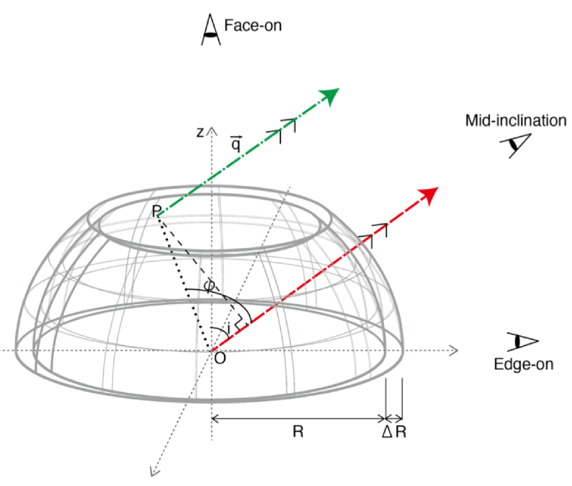
Figure 1: Assumed geometry of the ambient scattering medium and photon paths in our simulations. The scattering medium (grey solid line) is a ring-shaped part of the upper-half of a spherical shell, whose thickness ($\Delta R$) is $0.1R$. The point $P$ is the location where the photon interacts last in the shell, and $\vec{q}$ is a velocity vector the photon has. $i$ is the inclination angle and $\phi$ is the scattering angle. The red dashed/green dot-dashed lines show paths of the primary/reprocessed photons toward the line-of-sight.

We assume a simplified geometry, in which photons are emitted radially from a central point source (though in practice, this should have finite extent, which we assume is $5-10\,R_{g}$). We assume that the scattering medium is a section of a spherical shell (Fig. 1). The shell radius is from $R=100\,R_{g}$ to $110\,R_{g}$ across zenith angles $45^{\circ}$–$90^{\circ}$ (i.e., $\Omega/2\pi=0.7$). Photons emitted downwards are assumed to be blocked by the accretion disc. These will give an additional contribution to the lagged emission but here we are interested in the signatures of larger scale reflecting material so we neglect this. We assume $M_{\mathrm{BH}}=10^{7}\,M_{\odot}$, which means that the light-travel time to the shell is 5000 s. We note that the simulational results simply scale with $M_{\rm BH}$.

We consider two cases for the shell dynamics. We first explore what happens with a static shell, and secondly assume that the shell is formed by a wind. Typically, winds have outflow velocity similar to the escape velocity from its launch point, i.e. $0.14c=42,000$ km s^-1 for a launch radius of $100R_{g}$ (Tombesi et al. 2011). We assume that the turbulent velocity is $1000$ km s^-1 (Hagino et al. 2015). We set the hydrogen radial column density ($N_{\mathrm{H}}$) of the shell as $2\times 10^{23}\,\mathrm{cm}^{-2}$. Incident photons have a power-law spectrum whose photon index is 2. The number of input photons is $7\times 10^{8}$ in each case, injected as a delta function in time from 2–50 keV. Time-lags in the soft energy band ($<2$ keV) is also important (e.g., Fabian et al. 2009), but we do not treat this band because we now focus on the Fe-K feature around 5–8 keV and most of the soft photons are absorbed by the shell for our assumption of neutral material.

Fig. 1 shows the assumed geometry. The red dashed line shows the path of primary X-ray photons which pass through the shell on the line of sight to the observer. These have unit vector is $\vec{q}$. Other photons emitted along this path are absorbed or scattered in the shell and do not reach us. The green dot-dashed line shows the path of a reprocessed photon which does reach the observer. The point $P$ is the location where the photon interacts last in the shell at a time $t_{\mathrm{P}}$ after being emitted from the central source, no matter how many times it has been scattered previously. This photon has a time-delay of $t_{\mathrm{P}}-(\vec{P}\cdot\vec{q})/c$. Since MONACO keeps track of $t_{\mathrm{P}}$, $\vec{P}$ and $\vec{q}$, we can calculate the time-delay of each scattered photon relative to the direct photons as well as a scattering angle $\phi\equiv\arccos(\vec{p}\cdot\vec{q})$, where $\vec{p}$ is a unit vector of $\vec{P}$.

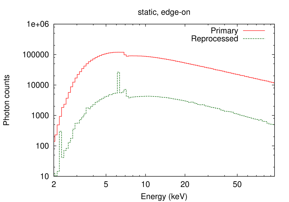
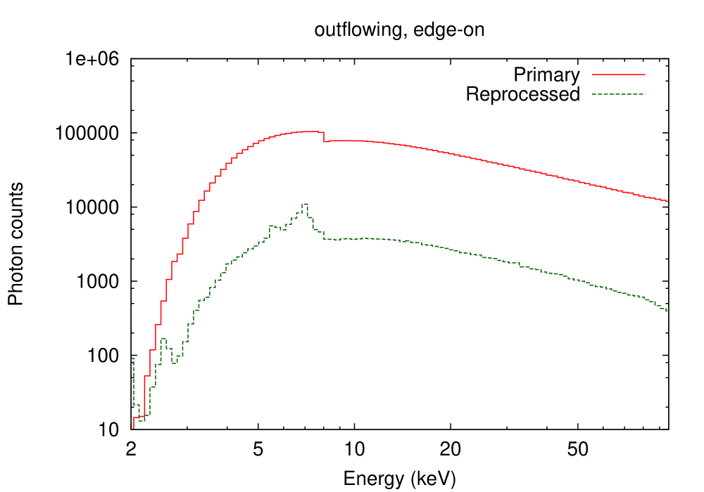
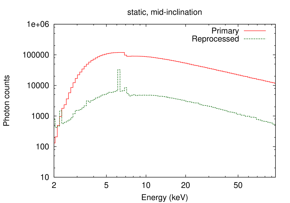
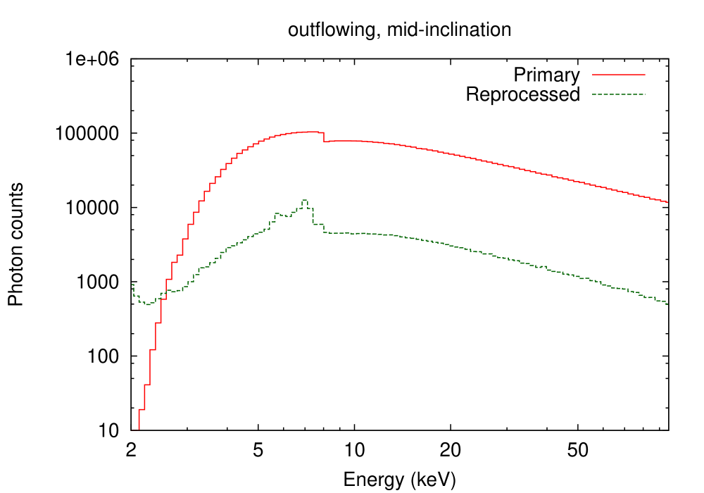
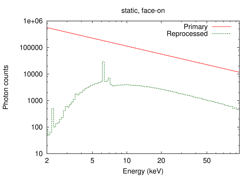
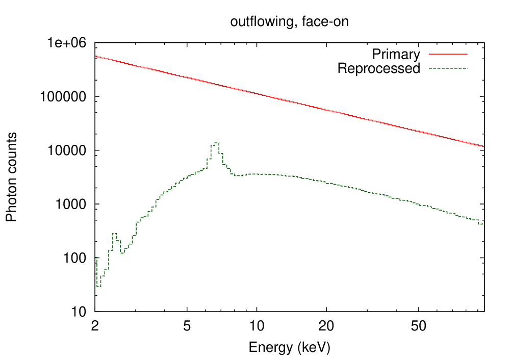
Figure 2: Energy spectra of primary/reprocessed components with different inclinations for each of the static shell (left) and the outflowing shell (right). Each energy-bin-width is made logarithmically equal ($\Delta\log E\,({\rm keV})=0.017$). Note that the reprocessed photons are dominant below $\sim 3$ keV in the outflowing mid-inclination case, which significantly affects the energy/frequency dependent lag features.

In this paper we assume a fixed size scale and the geometry as shown in Fig. 1. However, it is fairly simple to assess the impact of these parameter choices. The reprocessed fraction is set by the total solid angle of the reprocessing material and its optical depth, $\tau=n\sigma_{\rm T}\Delta R$, so that

$$f_{\rm rep}\sim\frac{\Omega}{2\pi}\tau\propto(1-\cos\theta_{\rm op})(n\Delta R),$$ (1)

where $\theta_{\rm op}$ is the half opening angle of the torus and the total column density in the wind is $N_{\rm H}=n\Delta R$. Thus changing the geometry from a spherical shell to a cylinder makes very little difference as long as $\theta_{\rm op}$ stays constant. The scattered fraction scales with total column density in the wind, so the fraction of lagged photons will depend linearly on $N_{\rm H}$. The delay-time ranges are from $\min\{0,R/c\,[1-\sin(\theta_{\rm op}+i)]\}$ (near side of the wind to the observer) to $R/c\,(1+\sin i)$ (far side) where $i$ is the zenith angle, so these depend linearly on the scale of the scatter. Thus the results shown here can be easily scaled to give an approximate result for changes in $R$, $\theta_{\rm op}$, and $n\Delta R$.

We show results along three different inclination angles, collecting photons in $\cos i$ ranges between 14/15 and 15/15 (face-on), between 7/15 and 8/15 (mid-inclination, which just intercepts the wind for our assumed $\theta_{\rm op}=45^{\circ}$), and between 0/15 and 1/15 (edge-on).

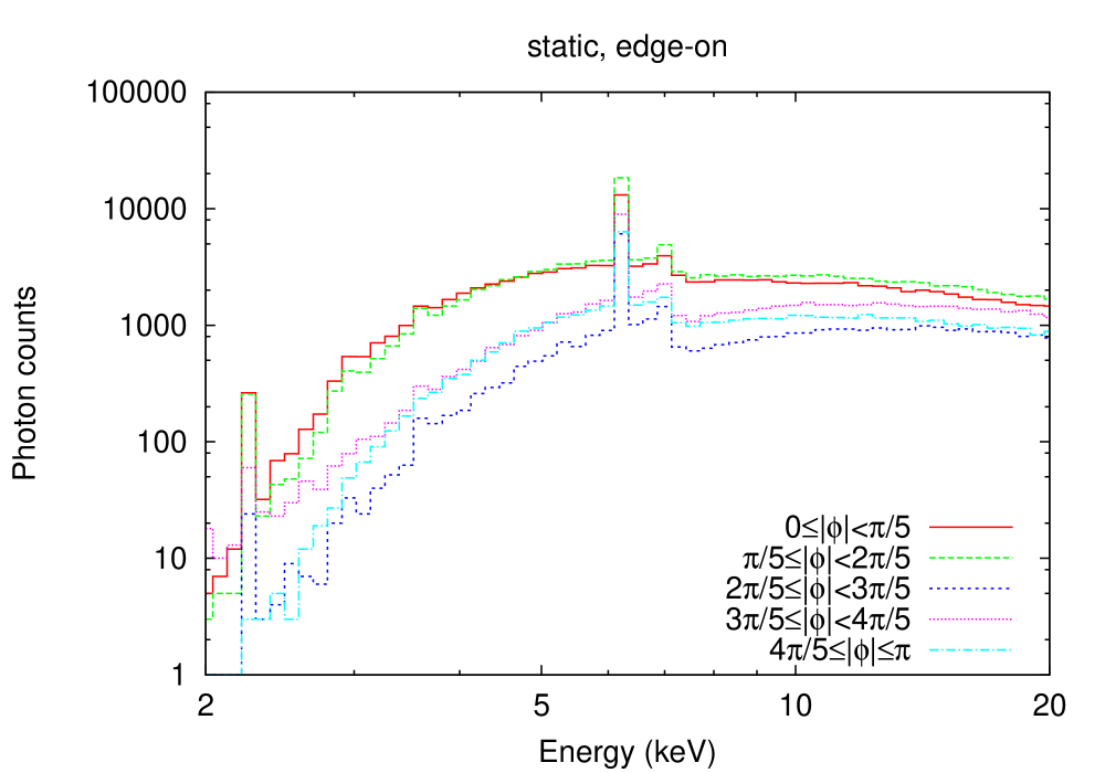
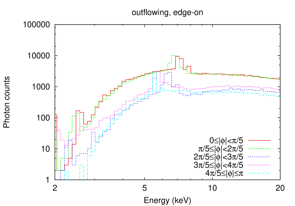
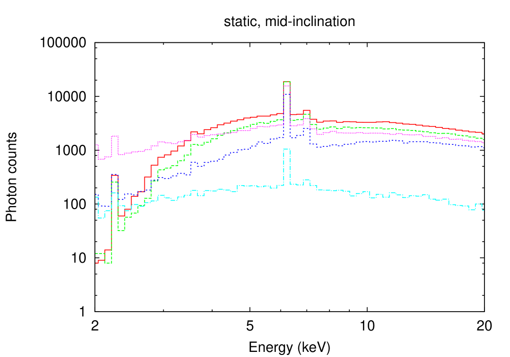
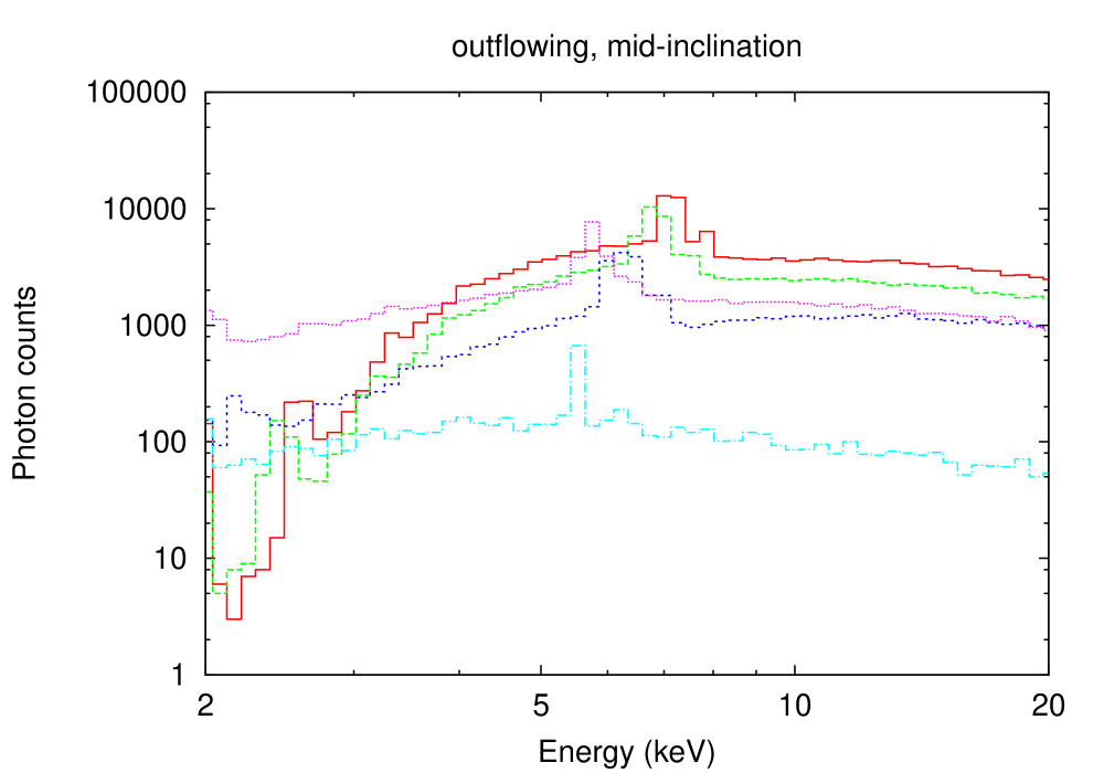
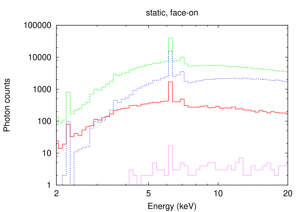
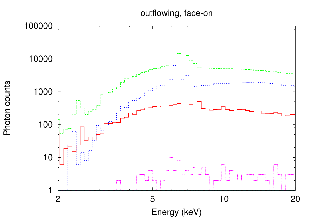
Figure 3: Energy spectra of the reprocessed components with different scattering angles ($\phi$), for each of the static shell (left) and the outflowing shell (right). The scattering angles are shown in the top panels.

3 Results

3.1 Spectra and transfer functions

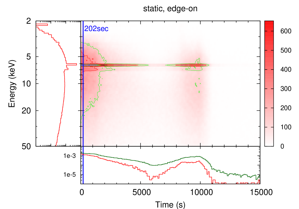
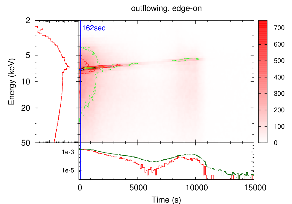
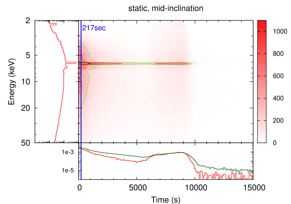
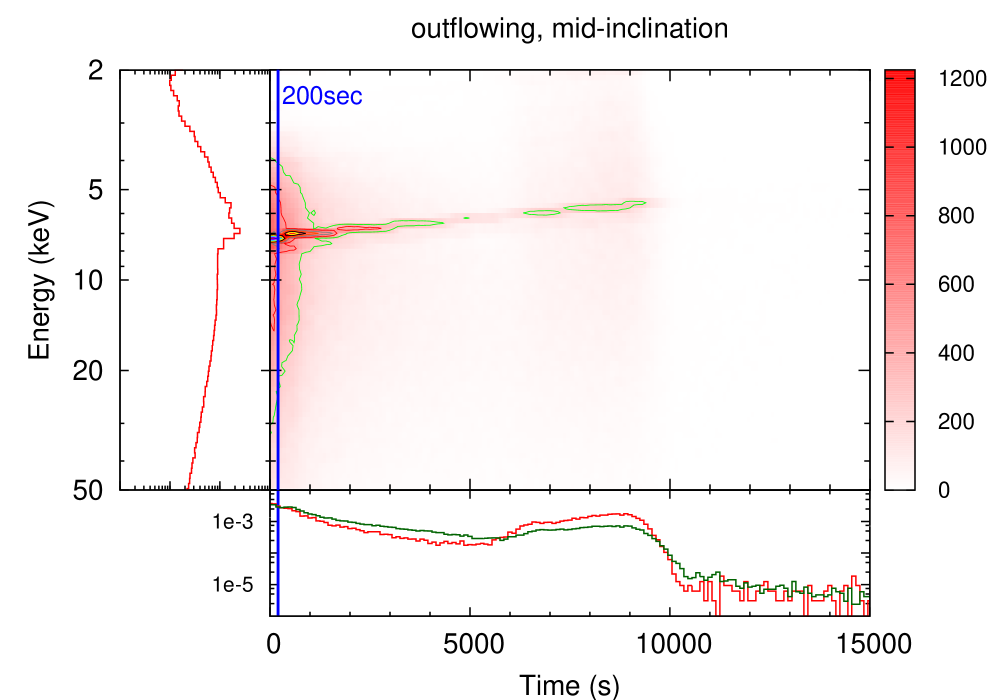
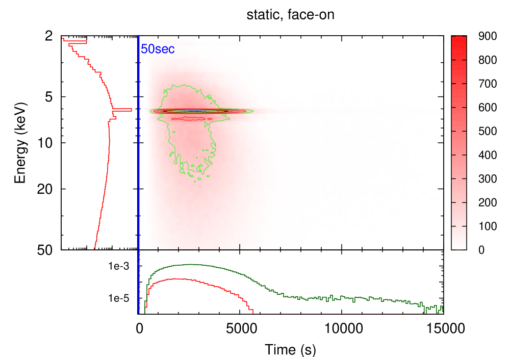
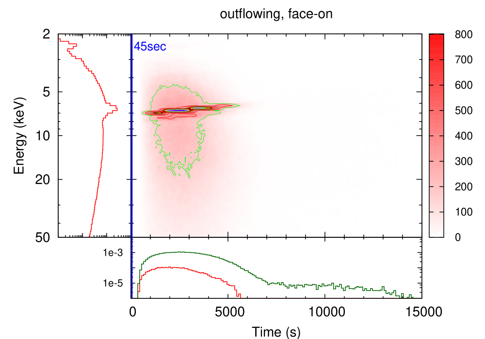
Figure 4: Main panels: Two dimensional transfer function $R(E,t)$ for the static (left) and wind (right) geometries for a distant shell at $R=10^{2}\,R_{g}$ around the $M_{\mathrm{BH}}=10^{7}\,M_{\odot}$ black hole ($R/c=5000$ s), at different inclination angles. The green contour shows where the count is 0.1 of the peak count. The blue vertical lines show the average delay time of all photons including primary ones. This is much smaller than $R/c$ as there are many more primary photons with zero lag than reprocessed photons with lag $\sim R/c$. The contour plots show where the response is at one-tenth of the peak count. The left panel on each plot shows the two dimensional response integrated over time, giving the reprocessed spectra. The bottom panel on each plot shows the two dimensional response integrated over the 3-5 keV (red) and 5-7 keV (green) energy bands, normalised with respect to the primary component.The difference in response at these two energies gives the observed lags between these two bands.

The resultant spectra from the Monte-Carlo simulations have two components; the primary one without time delay and the reprocessed one with a range of time delays. Fig. 2 shows these spectral components for the three inclination angles, for each of the static shell and the outflowing shell. The primary component (red lines) in the edge-on and mid-inclination case are strongly absorbed by the near side of the shell in the line of sight. The absorption in the soft energy band is stronger in the outflowing shell, because the source spectrum is redshifted to lower energies in the wind rest frame due to the Doppler shift. The reprocessed components (green lines) have fluorescent Fe-K lines at rest energies of 6.40 keV and 7.05 keV, an Fe-K edge at 7.1 keV, and a Compton hump above $\sim$20 keV. The Fe-K features in the outflowing shell are broadened, whereas they are sharp in the static shell.

Fig. 3 shows the reprocessed spectra for the static and outflowing cases for different scattering angles ($\phi$). This is mainly determined by the azimuthal angle of the point of last scattering, so this also sets the light-travel time lag. Photons with the longest lag time come from the far side of the wind so these are redshifted, whereas those with the shortest lag time are from the near side of the wind, so are blueshifted, while photons from the sides, with light travel time $\sim R/c$ are at the rest energy (though this will change if rotation of the wind is included). The superposition of these different Fe-K energies gives a broad line feature in the integrated response (Fig. 2, right panels).

In the edge-on case, photons in the soft energy bands are absorbed in all $\phi$ values. In the mid-inclination case, soft photons are not absorbed when $\phi$ gets larger as the far side of the shell can be seen directly even when the central source is obscured. In the face-on case, there are few photons whose $\phi$ is larger than $3\pi/5$. When an incident photon is emitted in the $x$ direction, $\vec{p}=(-1,0,0)$, and $\vec{q}=(\sqrt{29}/15,0,14/15)$, the maximum $\phi$ value is 111^∘.04, only slightly larger than $3\pi/5\,\mathrm{rad}=108^{\circ}$.

Fig. 4 shows counts of reprocessed photons in each time- (bin size of $100$ s) and energy-bin (bin size of $\Delta\log E\,({\rm keV})=0.017$) after the delta function continuum injection at $t=0$. This corresponds to the “two-dimensional transfer function” times the input photon spectrum. The left panels show projection on the $y$-axis, which gives the total energy spectrum of all the reprocessed photons. This picks out the energy bands of iron emission lines and Compton hump where the reprocessed photons are concentrated. The bottom panels plot counts of the reprocessed photons in 3–4 keV (red) and 5–7 keV (green) energy bands against the delay time. This corresponds to the response function in these bands (see e.g. Epitropakis et al. 2016). The measured lag between these bands is the difference between these two responses.

It is easy to see that the normalisation of the response is higher in the 5–7 keV band than in the 3–4 keV band for all simulations except for the outflowing, mid inclination case discussed previously. Thus the hard band will lag behind the soft as it has a higher contribution from the reprocessed flux. In both the edge-on and the mid-inclination cases, the response functions have two peaks, the first from 0–4000 s ($\lesssim 1R/c$) from scattering on the near side of the shell with a small scattering angles $\phi$, and the second peak at $\sim 9000$ s ($\simeq 2R/c$) from scattering on the far side of the shell with large $\phi$. These two merge into a single peak for the face-on case. These all span the range in lag times predicted in Section 2, i.e., $\sim 0-2R/c$ for edge on inclination and $\sim(1-\sin\theta_{\rm op})R/c-R/c$ for face on.

The blue vertical lines show the average delay time, i.e., the sum of all the reprocessed photons at all energies times their lag time, divided by the total number of photons (primary plus reprocessed over the entire energy band). The number of reprocessed photons is much less than that of the primary photons, and thus the average delay time is much shorter than the light-travel time of the reprocessed photons (dilution effect). In the edge-on and mid-inclination cases, the average delay time is $\sim$200 s, corresponding to $4\,R_{g}/c$. This is much shorter than the light-travel time from the source to the reflection shell by more than one order of magnitude. In the face-on case, the average delay time is even shorter, $\sim$50 s, which corresponds to $R_{g}/c$, because there are more primary photons and thus the dilution effect is more significant.

3.2 Lag-frequency plot

The frequency-dependent lag, $\tau(f)$, is defined as

$$\begin{split}\tau(f)&=\mathrm{arg}[C(f)]/(2\pi f)\\ C(f)&=\mathcal{S}(f)\mathcal{H}^{*}(f),\end{split}$$ (2)

where ^∗ denotes complex conjugate and $\mathcal{S}(f)$ and $\mathcal{H}(f)$ are Fourier transforms of soft- and hard-band light curves, $s(t)$ and $h(t)$ (Vaughan & Nowak 1997; Nowak et al. 1999), which is called as a cross spectrum. We use the standard convention that a positive lag means that photons in the hard band lag behind those in the soft band (e.g., Kara et al. 2013a). In other words, $s(t)$ is a light curve in a reference band, and $h(t)$ is the one in an energy band of interest.

An observed light curve at a given energy bin $E$ is expressed as the sum of the primary emission and the reprocessed emission. The primary emission is expressed as $P(E)g(t)$, where $P(E)$ is the (power-law) spectrum of the primary component and $g(t)$ is the intrinsic flux variability, which is assumed to have no $E$-dependence, i.e., the continuum varies only in normalisation. We define $R(E,k)$ as photon counts of the reprocessed component in each energy-bin ($E$) and time-bin ($k$), which is shown in Fig. 4. The reprocessed emission is expressed as $\sum_{k=0}^{k_{\rm max}}R(E,k)g(t-kt_{\rm bin})$, where $t_{\mathrm{bin}}$ is a time bin-size of the light curve ($=100$ s in this paper). We take $k_{\rm max}=400$, so we consider lags between 0–40,000 s. Here, the light curve at a given energy bin $E$ is written as

$$l(E,t)=P(E)g(t)+\sum_{k=0}^{k_{\rm max}}R(E,k)g(t-kt_{\rm bin}),$$ (3)

and its Fourier transform is expressed as

$$\mathcal{L}(E,f)=P(E)\mathcal{G}(f)+\sum_{k=0}^{k_{\rm max}}R(E,k)\exp[-2\pi i(kt_{\mathrm{bin}})f]\mathcal{G}(f),$$ (4)

where $\mathcal{L}(E,f)$ and $\mathcal{G}(f)$ are Fourier transforms of $l(E,t)$ and $g(t)$. Thus the soft- and hard-band light curves and their Fourier transforms are expressed as

$$\begin{split}s(t)&=\sum_{E\in{\rm\,soft\,band}}l(E,t)\\ h(t)&=\sum_{E\in{\rm\,hard\,band}}l(E,t),\end{split}$$ (5)

and

$$\begin{split}\mathcal{S}(f)&=P_{s}\mathcal{G}(f)+\sum_{k}R_{s}(k)\exp[-2\pi i(kt_{\mathrm{bin}})f]\mathcal{G}(f)\\ \mathcal{H}(f)&=P_{h}\mathcal{G}(f)+\sum_{k}R_{h}(k)\exp[-2\pi i(kt_{\mathrm{bin}})f]\mathcal{G}(f),\end{split}$$ (6)

where $P_{s}=\sum_{E\in{\rm\,soft\,band}}P(E)$, $R_{s}(k)=\sum_{E\in{\rm\,soft\,band}}R(E,k)$, and $P_{h}$ and $R_{h}(E)$ are those in the hard band. Therefore, equation (2) is calculated as

$$C(f) =\mathcal{S}(f)\mathcal{H}^{*}(f)$$

$$=\left(P_{s}+\sum_{k}R_{s}(k)\exp[-2\pi i(kt_{\mathrm{bin}})f]\right)$$

$$\>\>\>\>\>\>\left(P_{h}+\sum_{k}R_{h}(k)\exp[2\pi i(kt_{\mathrm{bin}})f]\right)|\mathcal{G}(f)|^{2}$$ (7)

and

$$\tau(f) =\frac{1}{2\pi f}\;\mathrm{arg}\left[\left(P_{s}+\sum_{k}R_{s}(k)\exp[-2\pi i(kt_{\mathrm{bin}})f]\right)\right.$$

$$\>\>\>\>\>\>\>\>\>\>\>\>\>\>\>\>\>\>\>\>\>\>\>\left.\left(P_{h}+\sum_{k}R_{h}(k)\exp[2\pi i(kt_{\mathrm{bin}})f]\right)\right].$$ (8)

Note that the frequency-dependent lag amplitudes do not depend on the functional form of the intrinsic variation, as long as the lags are caused by the reverberation. Hereafter, we calculate lags based on equation (8).

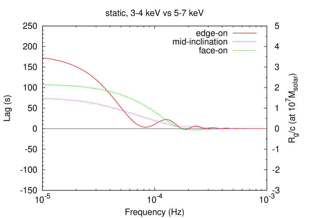
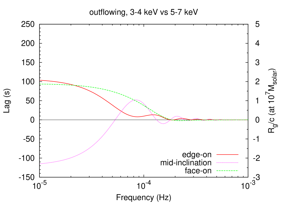
Figure 5: Lag-frequency plots when comparing 3-4 keV with 5-7 keV, derived from the Monte-Carlo simulation. Positive means hard lags, and vice versa.

Fig. 5 shows the lag-frequency plots, comparing a soft band (3–4 keV, where there is (generally) least contribution from the reprocessed component so that this is the best estimator of the continuum light curve; Fig. 2) with a hard band (5–7 keV, where the Fe-K emission peaks). In all cases except for the outflowing mid-inclination case, hard lags are seen with an amplitude of $\lesssim 150$ s, which is much shorter than the light-travel time to the shell (5000 s) and comparable to the weighted average delay time (Fig. 4). In the outflowing mid-inclination case, soft lags with an amplitude of $\sim 100$ s are seen because the reference 3–4 keV band has a higher fraction of reprocessed flux in this case than the others, so the “continuum” band is actually more dominated by lagged photons than the other cases. The lags are attenuated in all the cases for frequencies $>2\times 10^{-4}$ Hz, because variations on timescales faster than $R/c$ are smeared by the light-travel time across the shell.

We can get a useful analytic expression for the dilution by approximating the full response function by a single (average) intrinsic delay time, $\Delta\tau$($=k_{0}t_{\rm bin}$). Then equation (8) can be evaluated in a simple way as equation (5) becomes

$$\begin{split}s(t)&=P_{s}g(t)+R_{s}g(t-\Delta\tau)\\ h(t)&=P_{h}g(t)+R_{h}g(t-\Delta\tau),\end{split}$$ (9)

where $R_{s}$ and $R_{h}$ are the reprocessed component in the soft- and hard-band. In this case, $\tau(f)$ is calculated as

$$\tau(f) =\frac{1}{2\pi f}\mathrm{arg}\left[\left(P_{s}+R_{s}\exp[-2\pi i\Delta\tau f]\right)\left(P_{h}+R_{h}\exp[2\pi i\Delta\tau f]\right)\right]$$

$$=\frac{1}{2\pi f}\arctan\left(\frac{(P_{s}R_{h}-R_{s}P_{h})\sin(2\pi\Delta\tau f)}{P_{s}P_{h}+R_{s}R_{h}+(P_{s}R_{h}+R_{s}P_{h})\cos(2\pi\Delta\tau f)}\right).$$ (10)

In the $f\rightarrow 0$ limit,

$$\tau(f\rightarrow 0)=\frac{P_{s}R_{h}-R_{s}P_{h}}{(P_{s}+R_{s})(P_{h}+R_{h})}\Delta\tau=\mathrm{DF}\Delta\tau,$$ (11)

where the dilution factor DF can be calculated directly from the primary and reprocessed emission in each band. For example, when we use the parameters of the static edge-on case, then the soft band (3–4 keV) counts in the primary and reprocessed flux give $P_{s}=34.1$ and $R_{s}=1$, while the hard band (5–7 keV) has $P_{h}=111.6$ and $R_{h}=7.2$ (see Fig. 2), so ${\rm DF}=3.17\times 10^{-2}$. This predicts that DF reduces the observed lags by more than one order of magnitude. The mean intrinsic lag is of order $\Delta\tau\sim R/c=5000$ s, so this predicts an observed lag at low frequencies of $158$ s, which is very close to the $\sim 170$ s seen in the right panel of Fig. 5 for the edge-on case (red-solid line) as $f\to 0$. The difference comes from the mean intrinsic lag time being different from $R/c$ by a small factor (see the energy-compressed response in Fig. 4).

Equation (11) explicitly shows that the measured lag amplitudes are not a direct diagnostic of the size scale of the region; indeed they depend on the relative contribution of primary and reprocessed emission in each band. However, the frequency at which the lags go to zero is a much more robust constraint. For the delta-function approximation, equation (10) shows that this occurs where $2\pi\Delta tf=n\pi$ where $n$ is an integer, so the first zero crossing picks out $f_{0}=1/(2\Delta t)=c/2R$ Hz. Fig. 6 illustrates the light-travel time dependence of the lag frequencies, which is analytically calculated from equation (10) for different size scales of the reprocessor. The lags drop to zero at $f_{0}$, giving a clear diagnostic of the intrinsic size scale, and then oscillate around zero with decreasing amplitude (see also Fig. 21 of Uttley et al. 2014). The observed lag frequencies are $\sim 10^{-4}\,(10^{7}M_{\odot}/M_{\rm BH})$ Hz, which corresponds to $R=100\,R_{g}$. This means that materials located at $R\lesssim 100\,R_{g}$ contribute to the observed lag features.

However, the real response function covers a range in timescales from $\tau_{\rm min}<t<\tau_{\rm max}$ (see Fig. 4) rather than being a delta function at a single response time. We repeat the analysis assuming uniform response (a top-hat function: Appendix A). The spectral dilution factor is unchanged, so the lag as $f\to 0$ is the same as before (see also Fig. 21 of Uttley et al. 2014). However, the finite width of the response smooths out the oscillations around zero at high frequencies, and increases the attenuation so that the response drops more gradually. In the limit of a top hat from $0-2R/c$, the response never becomes negative, so there is no zero crossing, but there is still a minimum close to $\sim f_{0}$ (as shown in Fig. 5 where the relevant response shown in Fig. 4 is approximately a top hat from $0-2R/c$).

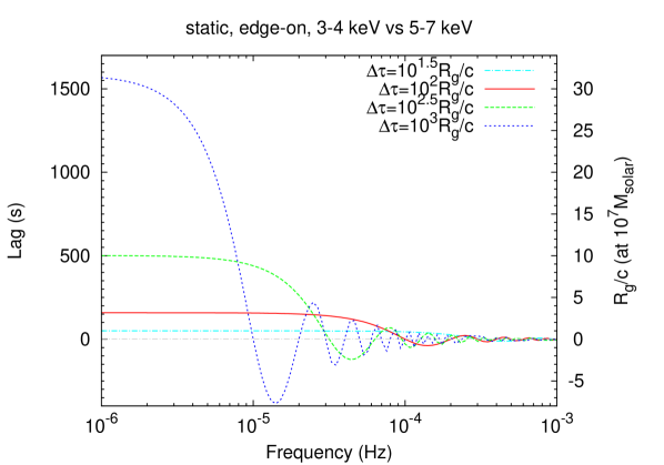
Figure 6: Lag-frequency plots with different size scales for the reprocessor assuming that the response is a delta-function at $R/c$. Parameters of the static edge-on case are used. The time delay $\Delta\tau$ gets shorter from top to bottom at $10^{-6}$ Hz.

3.3 Lag-energy plot

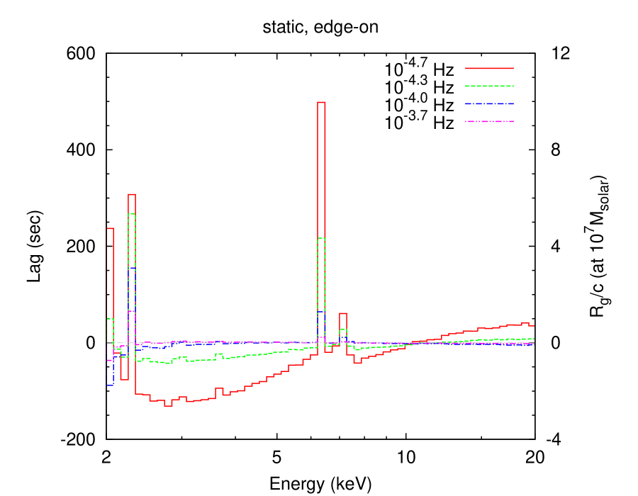
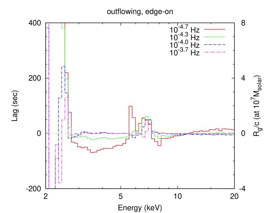
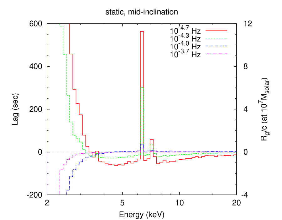
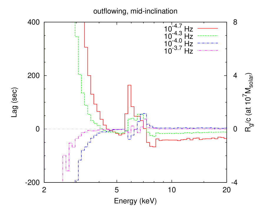
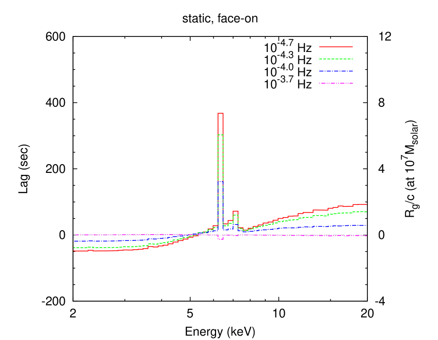
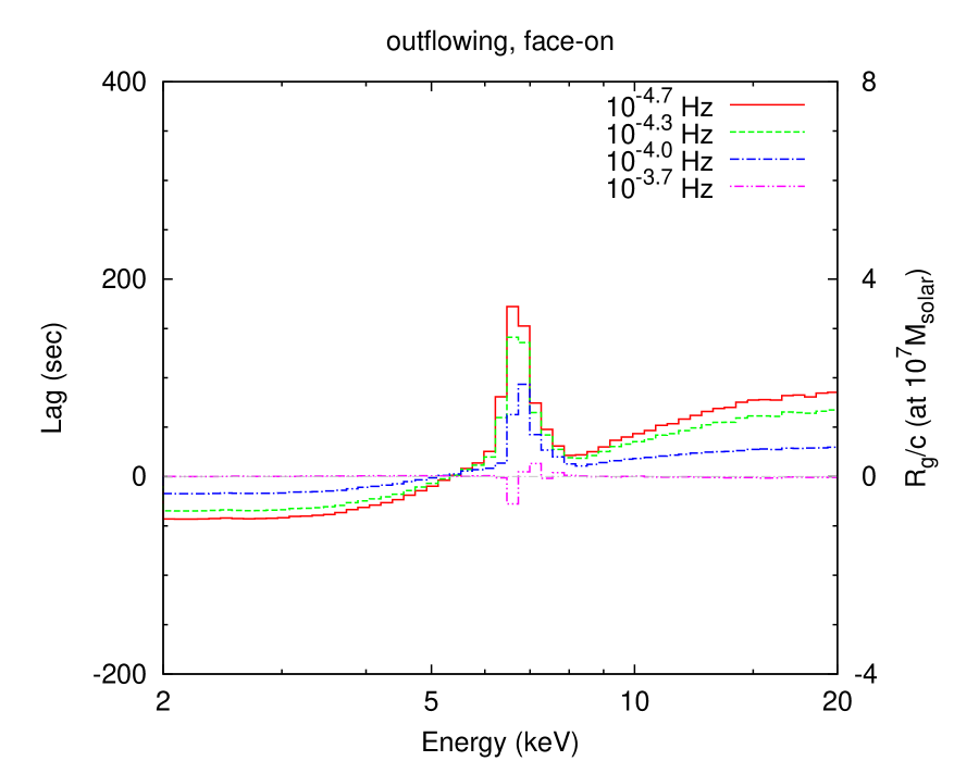
Figure 7: Lag-energy plots at various frequencies derived from the Monte-Carlo simulation.

We use the same formalism to describe the lag-energy plots. We use each energy bin as a band of interest $h(t)$ and the entire 2–20 keV (except for the energy bin of interest) as a reference band $s(t)$, to get maximum statistics (e.g., Uttley et al. 2014; Kara et al. 2016). Fig. 7 shows the lag-energy plots derived over four different frequencies to illustrate how this changes as a function of variability timescale. The Fe-K lag timescale (as well as all other lag features) become smaller as the frequency increases past $f_{0}=c/(2R)$ as the light travel time smears out faster variability. For lower frequencies, narrow Fe-K lines are seen from the static shell, while the line feature is smaller in lag and broader in energy for the wind. The large lags are seen in the soft energy band because the primary photons are heavily absorbed by the neutral shell. Such large lags would disappear when we consider ionised materials.

In the low frequency limit ($f\to 0$) the lags as a function of energy including the effect of dilution can be calculated analytically. Appendix B1 shows that the lag as a function of energy, $\tau(E)$, can written as

$$\Delta\tau(E)={\rm DF}(E)(f\rightarrow 0)\Delta\tau\approx\Bigl{(}\frac{R(E)}{P(E)}-\frac{R_{\rm tot}}{P_{\rm tot}}\Bigr{)}\Delta\tau$$ (12)

where $\Delta\tau$ is again the mean intrinsic lag of $R/c\sim 5000$ s. The measured lag times on the lowest frequency lag-energy plots are indeed close to these values: at the iron line energy then for the outflowing, edge on geometry this equation predicts that $\Delta\tau(6.8~{}{\rm keV})\sim 0.029\times\Delta\tau\sim 150$ s (see Appendix B.1 and Fig. 9). The iron line feature is narrow in the static case, so the lags at the iron line energy are longer as the lagged line photons are concentrated in a single energy bin so the effect of dilution is not so marked.

At higher frequencies, the iron line lag becomes smaller as the fast variations are smeared out by the light-travel time across the shell (see Fig. 6) in both the outflowing and static geometries, going towards zero as the frequency increases towards $2\times 10^{-4}$ Hz. For the static case, the lag-energy at frequencies approaching this limit shows a simple decrease in amplitude around zero. However, for the outflow, the line energy correlates with $\phi$, which correlates with the lag time. Hence the centroid energy of the broad Fe-K line in the lag-energy plot shifts depending on the variability timescale. Long variability times are required to see the longest lags, which come from material on the far side of the shell, where the line is redshifted. On the other hand, material on the near side of the shell, where the line is blueshifted, can respond to the shorter variability timescales. Thus the lag-energy plots for the outflowing shell have the line energy shifting from red to blue as the variability timescale decreases, correlated with decreasing line amplitude as the shell contributes less at higher frequencies. This is the first demonstration that a wind can also produce changes in iron line profile with Fourier frequency in lag-energy spectra.

4 Discussion

Reverberation techniques were first used in AGN to try to constrain the geometry of the broad line region. In this case the line can be spectrally separated from the continuum, and the observed lags directly show the difference of the light-travel time between the illuminating source and the scattering materials (e.g., Peterson 1993). However, in X-ray reverberation, both the continuum and the lagged emission share the same energy band, and thus the observed lag does not correspond to the light-travel time. In fact, Figs. 4 and 5 show that the average delay times of the simulated photons are much shorter than the light-travel time to the scattering medium because the primary continuum photons are dominant even in the Fe-K energy band. In other words, the primary photons “dilute” the lag amplitude of the reprocessed photons, reducing the observed lags in both lag-frequency and lag-energy plots. As was already stressed by several authors (e.g., Miller et al. 2010a; Kara et al. 2013b; Uttley et al. 2014; Gardner & Done 2014), the observed lag time is not a clean diagnostic of the size of the region. Instead, it depends on the dilution factor, which is given by the spectral decomposition, and this is generally not unique. Dilution of the lag exists in both lag-frequency and lag-energy plots. This dilution depends on the amount of reprocessed emission in the reference band, as well as the amount of primary emission in the lagged band. Thus the short lag times observed at the Fe-K line energy in several objects (Kara et al. 2016) do not necessarily indicate that this is produced very close to the event horizon of the black hole.

Instead, we have argued that the frequency at which the lags are attenuated is a more robust estimator of the size scale, with the reverberation lags being seen below $\sim c/R$ Hz. Thus even the most extreme object, 1H 0707–495, where the Fe-K band lag is of order of 50 s, has reverberation lags which are detected up to $7\times 10^{-3}$ Hz (Kara et al. 2013a). This indicates a firm upper limit to location of the reverberating region of $143$ s, i.e., $\sim 14\,R_{g}$. This size scale is of the same order as the launching radius of a super-Eddington wind inferred from the data, $\sim 20\,R_{g}$ (Done & Jin 2016), and the observed broad profile in the lag-energy plot can be naturally explained by the Doppler shifts in the wind.

The equivalent width of Fe-K emission line in our calculation is $\sim 50-100$ eV with Doppler broadening of $\sim 0.7$ keV (for edge-on and mid-inclination) and $\sim 0.3$ keV (for face-on) in the outflowing cases, which is less than the observed Fe-K skewed emission line. Whereas scattering on the shell cannot produce the observed Fe-K spectral feature, the Fe-K absorption edge due to the shell may mimic the broad spectral feature if the shell is clumpy and partially covers the X-ray source, (e.g., Tanaka et al. 2004; Mizumoto et al. 2014). Hagino et al. (2016) also argued that the blueshifted absorption line due to disc winds can mimic the spectral feature in 1H 0707–495. In these manners, we suggest that the distant materials can explain both the energy spectra and the lag features in the Fe-K band simultaneously. Here we do not consider disc reflection for simplicity, but of course, disc within $100\,R_{g}$ must exist and affect the reverberation lags. Reverberation of the Compton hump seen in some targets (e.g., Zoghbi et al. 2014; Kara et al. 2015) might trace such disc reflection, because the hump expected by our picture is little.

The lag-energy plots show that the correlation of velocity with position as in a radial outflow leads to shifts in the line energy and amplitude. Such shifts are seen in NGC 4151 (Zoghbi et al. 2012), where at frequencies $\leq 2\times 10^{-5}$ Hz there is a distinct feature around the iron line energy, which becomes much broader, i.e., much less distinct at higher frequencies (see Figs. 2 and 7 of Zoghbi et al. 2012). This is similar to the behaviour of the line in the lag-energy spectra with an outflow shown in our Fig. 7 (right column, middle panel). The line response is strongly suppressed on frequencies smaller than $c/R$, so the data from NGC 4151 are then consistent with being from a wind at a few 100’s of $R_{g}$ rather than $\sim 5\,R_{g}$ as modelled by Cackett et al. (2014).

5 Conclusion

We calculate the X-ray reverberation lags produced by a quite distant matter around AGN via a Monte-Carlo simulation. In our simulations, the scattering material is assumed to be a neutral, part-spherical thin shell at $100\,R_{g}$ with the black-hole mass of $10^{7}\,M_{\odot}$, which can be either static or outflowing at $0.14c$. We compiled results for each simulation over three different inclination angles.

We found short-time ($\lesssim 150$ s) hard lags between a continuum (3–4 keV) and Fe-K band (5–7 keV) in the frequency range of $\lesssim 10^{-4}$ Hz, which is much shorter than the light-travel time (5000 s). The short lag amplitude compared to the light-travel time is explained by the dilution effect, where the majority of the photons in the Fe-K energy band are primary photons without time-delay, whereas the time-delayed reprocessed photons make a subtle contribution. The line is broadened in the lag-energy plots when the scattering material is an outflowing wind; photons scattered on the near side are blueshifted, whereas those on the far side are redshifted. This makes a broad feature with short lag time in lag-energy plots, similar to that seen in 1H0707-495. The correlation of line of sight velocity in the wind and lag time leads to shifts in the observed energy of the line as a function of frequency, similar to those seen in NGC 4151 (Zoghbi et al. 2012). Hence we show that the observed X-ray reverberation lag features can be produced by the outflowing matter such as disc winds at $\sim 100\,R_{g}$. This is a viable alternative geometry to a compact corona close to the event horizon of a high spin black hole.

Appendix A Response of a top-hat function

In §3.2, we derived equation (10) assuming that the reprocessed component can be represented by a single intrinsic delay time, or the response is a delta-function. However, this assumption is too simplified, because the response function (see bottom panels in Fig. 4) is not like a delta-function; it is rather like a top-hat function. In this section, we analytically evaluate the lags with response of the top-hat function.

First, we rewrite equation (5) as

$$\begin{split}s(t)&=P_{s}g(t)+R_{s}\int\!\!dt^{\prime}\psi_{s}(t^{\prime})g(t-t^{\prime})\\ h(t)&=P_{h}g(t)+R_{h}\int\!\!dt^{\prime}\psi_{h}(t^{\prime})g(t-t^{\prime}),\end{split}$$ (13)

where $R_{s}$ and $R_{h}$ show the reprocessed components in the soft- and hard-band, and $\psi_{s}$ and $\psi_{h}$ are normalised response functions ($\int\!\!dt\,\psi_{s}(t)=\int\!\!dt\,\psi_{h}(t)=1$). In this case,

$$\mathcal{S}(f)\mathcal{H}^{*}(f)=\{P_{s}+R_{s}\Psi_{s}(f)\}\{P_{h}+R_{h}\Psi^{*}_{h}(f)\}|\mathcal{G}(f)|^{2},$$ (14)

where $\Psi_{s}(f)$ and $\Psi_{h}(f)$ is a Fourier transform of $\psi_{s}(t)$ and $\psi_{h}(t)$. Under the assumption that $\psi_{s}(t)=\psi_{h}(t)=\psi(t)$, or $\Psi_{s}(f)=\Psi_{h}(f)=\Psi(f)=a(f)+ib(f)$, $\tau(f)$ is calculated as

$$\tau(f)=\frac{1}{2\pi f}\arctan\left(\frac{-b(P_{s}R_{h}-R_{s}P_{h})}{P_{s}P_{h}+R_{s}R_{h}+a(P_{s}R_{h}+R_{s}P_{h})}\right).$$ (15)

When the response is a top-hat function,

$$\psi(t)=\begin{cases}1/\Delta\tau&(\tau_{\rm min}\leq t\leq\tau_{\rm max})\\ 0&(\mathrm{otherwise}),\end{cases}$$ (16)

$\Psi(f)$ is written as

$$\Psi(f) =\frac{1}{-2\pi if\Delta\tau}\left(\exp[-2\pi if\tau_{\rm max}]-\exp[-2\pi if\tau_{\rm min}]\right)$$

$$=\frac{1}{2\pi f\Delta\tau}\left[\left\{2\cos\left(2\pi f\tau_{\rm ave}\right)\sin\left(2\pi f\frac{\Delta\tau}{2}\right)\right\}\right.$$

$$\>\>\>\>\>\>\>\>\>\>\>\>\>\>\>\>\>\>\>\>\>\>\left.-i\left\{2\sin\left(2\pi f\tau_{\rm ave}\right)\sin\left(2\pi f\frac{\Delta\tau}{2}\right)\right\}\right],$$ (17)

where $\tau_{\rm ave}=(\tau_{\rm max}+\tau_{\rm min})/2$ and $\Delta\tau=(\tau_{\rm max}-\tau_{\rm min})/2$. In a limit of $f\rightarrow 0$, we see lags on the longest timescale, so a finite width of the top-hat function can be ignored and the response can be treated as a delta function, and we can use the same dilution factor (equation 11). Fig. 8 illustrates the light-travel time dependence of the lag frequencies, with the top-hat function ($\tau_{\rm min}=0$ and $\tau_{\rm max}=2\Delta\tau$). The lags oscillate around zero at high frequencies, and almost disappear on $c/R$, which is same as the delta-function case (Fig. 6).

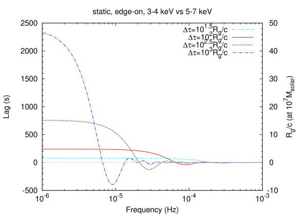
Figure 8: Same as Fig. 6, but the top-hat function is assumed ($\tau_{\rm min}=0$ and $\tau_{\rm max}=2\Delta\tau$ in equation 17).

Appendix B Details of the dilution effect

B.1 Dilution factor as a function of energy

The dilution factor is derived in equation (11) in the $f\to 0$ limit. The energy-dependent dilution factor ${\rm DF}(E)$ is similarly expressed as

$$\mathrm{DF}(E)=\frac{P_{\rm tot}R(E)-R_{\rm tot}P(E)}{(P_{\rm tot}+R_{\rm tot})(P(E)+R(E))},$$ (18)

where $P(E)$ and $R(E)$ are the primary and reprocessed components in the energy bin of interest, and $P_{\rm tot}$ and $R_{\rm tot}$ are those in the total energy band, like equation (10). Under the assumption that $R_{\rm tot}/P_{\rm tot}\ll 1$ and $R(E)/P(E)\ll 1$, equation (18) is approximated as

$$\mathrm{DF}_{\rm approx}(E)=\frac{R(E)}{P(E)}-\frac{R_{\rm tot}}{P_{\rm tot}}.$$ (19)

In other words, ${\rm DF}_{\rm approx}$ is calculated as difference between relative flux of the reprocessed component to the primary component in the energy bin of interest and that in the total energy band. These equations work very well to describe the lag-energy spectrum seen from the static shell at low frequencies. Fig. 9 shows comparison of the lag-energy plot in the low-frequency range with $\mathrm{DF}(E)$. We can see that $\tau_{f\to 0}(E)\simeq{\rm DF}(E)\Delta\tau\simeq{\rm DF}_{\rm approx}(E)\Delta\tau$, with only several differences around the line profile.

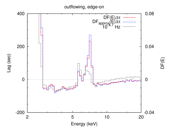
Figure 9: The plot of ${\rm DF}(E)\Delta\tau$ (red-solid, shown by equation 18), ${\rm DF_{approx}(E)\Delta\tau}$ (blue-dot-dashed, shown by equation 19), and the lag-energy plot in the outflowing edge-on case at $10^{-4.7}$ Hz (grey-dashed), which is same as the one in the right upper panel of Fig. 7). The right axis shows the ${\rm DF}(E)$ values.

In all the cases, both static and outflowing, the Fe-K lag amplitudes correspond to several $R_{g}/c$, much shorter than $R/c=100\,R_{g}/c$. Calculating this explicitly for the outflowing case, at $E=6.8\,{\rm keV}$ (slightly lower energy than the blue peak of the outflowing line) gives

$$\mathrm{DF}_{\rm approx}(E=6.8\,{\rm keV}) =\frac{R(E)}{P(E)}-\frac{R_{\rm tot}}{P_{\rm tot}}$$

$$=0.081-0.052$$

$$=0.029,$$ (20)

which means that the lag amplitude is diluted by almost two orders of magnitude (see Fig 9). The lag at the iron line energy in the lag-energy spectrum can be as affected by dilution as is the broader energy band used for the lag-frequency spectrum.

B.2 Separating lagged and primary emission

We have studied the dilution effect in the low-frequency limit in the above subsection (e.g., equation 19). In this subsection, we investigate the dilution effect in all the frequency ranges. We explained that lags are diluted because the primary and reprocessed components share the same energy band, so here we calculate lags when they do not share the same band. Since this is a simulation, we can separate out the lagged and primary emission. In an ideal situation, first, let us consider that a reference band has only primary emission, whereas an energy band of interest has the only reprocessed emission. In this case, the lag amplitudes are written as

$$\tau_{f}(E)=\frac{1}{2\pi f}{\rm arg}\left[P_{\rm tot}\sum_{k}R(E,k)\exp[2\pi ikt_{\rm bin}f]\right].\\$$

The resultant lag-energy plot is shown in Fig. 10(a). This plot is not affected by dilution and the lag amplitude is an order of $R/c=5000$ s, as expected, but it does have energy dependence due to the lag weighting of the numerator. We investigate this in the low-frequency limit, where

$$\tau_{f}(E) \xrightarrow[f\to 0]{}\frac{1}{2\pi f}{\rm arg}\left[\sum_{k}R(E,k)+iR(E,k)2\pi kt_{\rm bin}f\right]$$

$$=\frac{1}{2\pi f}\arctan\left(\frac{\sum_{k}R(E,k)2\pi kt_{\rm bin}f}{\sum_{k}R(E,k)}\right)$$

$$\to\frac{\sum_{k}kt_{\rm bin}R(E,k)}{\sum_{k}R(E,k)}.$$ (21)

In effect, the difference between the reprocessed emission lagged by $kt_{\rm bin}$ and the time averaged lagged spectrum produces the energy dependence.

Next, we explore the situation where the energy bin of interest contains the primary component as well as the reprocessed one. This has a very similar profile to the measured lag-energy plot (Fig. 10b), but the dilution effect takes place. In the low-frequency limit, this plot is expressed as

$$\tau_{f}(E)\xrightarrow[f\to 0]{}\frac{\sum_{k}kt_{\rm bin}R(E,k)}{P(E)+\sum_{k}R(E,k)}.$$ (22)

We can see that the $P(E)$ component in the denominator acts as a diluting factor. The plot is shifted by $\sim 150$ s because we ignored the reprocessed component in the reference band. Indeed, the effect of $R_{\rm tot}$ is estimated as $(R_{\rm tot}/P_{\rm tot})\tau$ from equation (19), and $R_{\rm tot}/P_{\rm tot}\simeq 0.053$ and $3000\,{\rm s}\times 0.053\sim 150$ s, where 3000 s is the average value of equation (21).

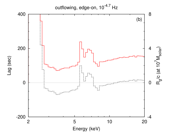
Figure 10: (a) The lag-energy plot when the reference band has only the primary component and the energy bin of interest has only the reprocessed component in the outflowing edge-on case at $10^{-4.7}$ Hz, derived from the Monte-Carlo simulation. (b) The one when the reference band has only the primary component but the energy bin of interest has both the primary and reprocessed components (red-solid). The grey dashed line is same as the one in Fig. 9.

References

- Agostinelli et al. (2003) Agostinelli S., et al., 2003, Nuclear Instruments and Methods in Physics Research A, 506, 250
- Allison et al. (2006) Allison J., et al., 2006, IEEE Transactions on Nuclear Science, 53, 270
- Arévalo & Uttley (2006) Arévalo P., Uttley P., 2006, MNRAS, 367, 801
- Cackett et al. (2014) Cackett E. M., Zoghbi A., Reynolds C., Fabian A. C., Kara E., Uttley P., Wilkins D. R., 2014, MNRAS, 438, 2980
- Chainakun et al. (2016) Chainakun P., Young A. J., Kara E., 2016, MNRAS, 460, 3076
- Done & Jin (2016) Done C., Jin C., 2016, MNRAS, 460, 1716
- Epitropakis et al. (2016) Epitropakis A., Papadakis I. E., Dovčiak M., Pecháček T., Emmanoulopoulos D., Karas V., McHardy I. M., 2016, A&A, 594, A71
- Fabian et al. (2009) Fabian A. C., et al., 2009, Nature, 459, 540
- Gardner & Done (2014) Gardner E., Done C., 2014, MNRAS, 442, 2456
- Gardner & Done (2015) Gardner E., Done C., 2015, MNRAS, 448, 2245
- Hagino et al. (2015) Hagino K., Odaka H., Done C., Gandhi P., Watanabe S., Sako M., Takahashi T., 2015, MNRAS, 446, 663
- Hagino et al. (2016) Hagino K., Odaka H., Done C., Tomaru R., Watanabe S., Takahashi T., 2016, MNRAS, 461, 3954
- Kara et al. (2013a) Kara E., Fabian A. C., Cackett E. M., Steiner J. F., Uttley P., Wilkins D. R., Zoghbi A., 2013a, MNRAS, 428, 2795
- Kara et al. (2013b) Kara E., Fabian A. C., Cackett E. M., Uttley P., Wilkins D. R., Zoghbi A., 2013b, MNRAS, 434, 1129
- Kara et al. (2014) Kara E., Cackett E. M., Fabian A. C., Reynolds C., Uttley P., 2014, MNRAS, 439, L26
- Kara et al. (2015) Kara E., et al., 2015, MNRAS, 446, 737
- Kara et al. (2016) Kara E., Alston W. N., Fabian A. C., Cackett E. M., Uttley P., Reynolds C. S., Zoghbi A., 2016, MNRAS, 462, 511
- Kotov et al. (2001) Kotov O., Churazov E., Gilfanov M., 2001, MNRAS, 327, 799
- Miller et al. (2010a) Miller L., Turner T. J., Reeves J. N., Lobban A., Kraemer S. B., Crenshaw D. M., 2010a, MNRAS, 403, 196
- Miller et al. (2010b) Miller L., Turner T. J., Reeves J. N., Braito V., 2010b, MNRAS, 408, 1928
- Mizumoto et al. (2014) Mizumoto M., Ebisawa K., Sameshima H., 2014, PASJ, 66, 122
- Mizumoto et al. (2018) Mizumoto M., Moriyama K., Ebisawa K., Mineshige S., Kawanaka N., Tsujimoto M., 2018, PASJ, accepted (arXiv: 1802.07554)
- Niedźwiecki et al. (2016) Niedźwiecki A., Zdziarski A. A., Szanecki M., 2016, ApJ, 821, L1
- Nowak et al. (1999) Nowak M. A., Vaughan B. A., Wilms J., Dove J. B., Begelman M. C., 1999, ApJ, 510, 874
- Odaka et al. (2011) Odaka H., Aharonian F., Watanabe S., Tanaka Y., Khangulyan D., Takahashi T., 2011, ApJ, 740, 103
- Peterson (1993) Peterson B. M., 1993, PASP, 105, 247
- Tanaka et al. (2004) Tanaka Y., Boller T., Gallo L., Keil R., Ueda Y., 2004, PASJ, 56, L9
- Tombesi et al. (2011) Tombesi F., Cappi M., Reeves J. N., Palumbo G. G. C., Braito V., Dadina M., 2011, ApJ, 742, 44
- Turner et al. (2017) Turner T. J., Miller L., Reeves J. N., Braito V., 2017, MNRAS, 467, 3924
- Uttley et al. (2014) Uttley P., Cackett E. M., Fabian A. C., Kara E., Wilkins D. R., 2014, A&A Rev., 22, 72
- Vaughan & Nowak (1997) Vaughan B. A., Nowak M. A., 1997, ApJ, 474, L43
- Wilkins et al. (2016) Wilkins D. R., Cackett E. M., Fabian A. C., Reynolds C. S., 2016, MNRAS, 458, 200
- Zhou & Wang (2005) Zhou X.-L., Wang J.-M., 2005, ApJ, 618, L83
- Zoghbi et al. (2011) Zoghbi A., Uttley P., Fabian A. C., 2011, MNRAS, 412, 59
- Zoghbi et al. (2012) Zoghbi A., Fabian A. C., Reynolds C. S., Cackett E. M., 2012, MNRAS, 422, 129
- Zoghbi et al. (2014) Zoghbi A., et al., 2014, ApJ, 789, 56