Universal thermodynamic properties of the intracluster medium over two decades in radius in the X-COP sample

Abstract

Context. The hot plasma in a galaxy cluster is expected to be heated to high temperatures through shocks and adiabatic compression. The thermodynamical properties of the gas encode information on the processes leading to the thermalization of the gas in the cluster’s potential well and on non-gravitational processes such as gas cooling, AGN feedback, shocks, turbulence, bulk motions, cosmic rays and magnetic field.

Aims. In this work we present the radial profiles of the thermodynamic properties of the intracluster medium (ICM) out to the virial radius for a sample of 12 galaxy clusters selected from the Planck all-sky survey. We determine the universal profiles of gas density, temperature, pressure, and entropy over more than two decades in radius, from 0.01$R_{500}$ to 2 $R_{500}$.

Methods. We exploited X-ray information from XMM-Newton and Sunyaev-Zel’dovich constraints from Planck to recover thermodynamic properties out to $2R_{500}$. We provide average functional forms for the radial dependence of the main quantities and quantify the slope and intrinsic scatter of the population as a function of radius.

Results. We find that gas density and pressure profiles steepen steadily with radius, in excellent agreement with previous observational results. Entropy profiles beyond $R_{500}$ closely follow the predictions for the gravitational collapse of structures. The scatter in all thermodynamical quantities reaches a minimum in the range $[0.2-0.8]R_{500}$ and increases outward. Somewhat surprisingly, we find that pressure is substantially more scattered than temperature and density.

Conclusions. Our results indicate that once accreting substructures are properly excised, the properties of the ICM beyond the cooling region ($R>0.3R_{500}$) follow remarkably well the predictions of simple gravitational collapse and require few non-gravitational corrections.

1 Introduction

Galaxy clusters are the largest bound structures in the Universe. In the hierarchical structure formation scenario, they grow from primordial density fluctuations to form the massive structures we observe today (e.g., Kravtsov & Borgani, 2012). Pristine gas falls into the dark matter potential and is progressively heated up to temperatures of $10^{7}-10^{8}$ K, such that the majority of the baryons end up in the form of a fully ionized plasma, the intracluster medium (ICM), which produces X-ray emission through bremsstrahlung radiation and line emission. In addition, photons of the cosmic microwave background (CMB) crossing galaxy clusters are subject to inverse Compton scattering off the hot ICM electrons. This produces a spectral shift in the CMB signal, the Sunyaev-Zel’dovich (SZ) effect (Sunyaev & Zeldovich, 1972), which is detectable at microwave wavelengths. X-ray emission and the SZ effect thus provide highly complementary diagnostics of the state of the ICM.

The thermodynamical properties of the ICM encode valuable information on the processes governing the formation and evolution of galaxy clusters. At first approximation, the state of the gas is determined by the properties of the gravitational potential and the merging history of the host halo alone. Gravitational collapse implies the existence of tight scaling laws between ICM properties and cluster mass (the self-similar model, Kaiser, 1986; Bryan & Norman, 1998) and non-radiative cosmological simulations predict that the scaled thermodynamical profiles of massive systems are nearly universal (e.g., Frenk et al., 1999; Borgani et al., 2005; Voit, 2005). Thus, the distribution of the thermodynamical properties across the ICM is a powerful tool for probing the formation of galaxy clusters. Deviations from gravitational collapse predictions can be used as a way to quantify the impact of non-gravitational physics such as gas cooling and feedback from supernovae and active galactic nuclei (AGN) (Tozzi & Norman, 2001; Kay et al., 2002; Borgani et al., 2004; Kravtsov et al., 2005; Gaspari et al., 2014) and to probe hydrodynamical phenomena induced by structure formation such as shocks, turbulence and bulk motions (Dolag et al., 2005; Rasia et al., 2006; Vazza et al., 2009; Burns et al., 2010), cosmic rays (Pfrommer et al., 2007), and magnetic fields (Dolag et al., 1999). In recent years, hydrodynamical simulations of increasing complexity have attempted to model simultaneously all known non-gravitational effects and to determine their impact on the structural properties of galaxy clusters (e.g., Le Brun et al., 2014; Hahn et al., 2017; Planelles et al., 2017; Barnes et al., 2017; Gaspari et al., 2018). These simulations highlight the role played by AGN feedback in maintaining the cooling/heating balance and regulating the star formation efficiency.

In the past decade, X-ray observations have provided constraints of increasing quality on the distribution of gas density (Croston et al., 2006; Eckert et al., 2012), temperature (De Grandi & Molendi, 2002; Vikhlinin et al., 2006; Pratt et al., 2007; Leccardi & Molendi, 2008), pressure (Arnaud et al., 2010), and entropy (Cavagnolo et al., 2009; Pratt et al., 2010) throughout the ICM. However, these observations sampled a radial range limited to less than half of the virial radius, and thus the majority of the cluster volume, and the entirety of the accretion region, remained unexplored. Thanks to its low instrumental background, the Suzaku satellite allowed us to extend the accessible radial range to the virial radius in a dozen clusters (e.g., Reiprich et al., 2013; Akamatsu et al., 2011; Simionescu et al., 2011, 2017; Walker et al., 2012a, b; Urban et al., 2014). Somewhat surprisingly, most studies find steeply decreasing temperature profiles and a flattening of the entropy at $R_{500}$ and beyond, at odds with the predictions of gravitational collapse. Possible explanations for these behaviors include biases in X-ray measurements caused by gas clumping (Nagai & Lau, 2011; Simionescu et al., 2011; Vazza et al., 2013; Roncarelli et al., 2013), non-equilibrium between electrons and ions (Hoshino et al., 2010; Avestruz et al., 2015), breakdown of hydrostatic equilibrium caused by turbulence and bulk motions (Lapi et al., 2010; Okabe et al., 2014; Avestruz et al., 2015; Khatri & Gaspari, 2016), or as-yet-unknown systematics in the subtraction of the Suzaku background. Clearly, accurate observational data out to the virial radius are required to understand the origin of these deviations.

Since the first X-ray observations of galaxy clusters it has become evident that clusters can be divided into two categories differing only in their central properties (Jones & Forman, 1984). The origin of these two populations is still unclear; however, several recent works (Rossetti et al., 2017; Lovisari et al., 2017; Andrade-Santos et al., 2017) point out that there is a clear difference between X-ray and SZ selected samples, also generating possible biases in the measured thermodynamic quantities.

In this paper, we present the universal thermodynamical properties of the galaxy clusters in the XMM Cluster Outskirts Project (X-COP), a sample of 12 massive, local galaxy clusters ($z<0.1$) with deep XMM-Newton and Planck data covering the entire azimuth out to the virial radius. Unlike previous studies that exclusively utilized the X-ray signal, we take advantage of the high signal-to-noise ratio of our clusters in the Planck survey (Planck Collaboration XXIX, 2014), and combine X-ray and SZ data to increase the precision of our measurements while keeping a good control of systematic errors. This method was applied to reconstruct the thermodynamical properties of a few clusters (Basu et al., 2010; Eckert et al., 2013; Adam et al., 2015; Ruppin et al., 2017), and we demonstrated the ability of XMM-Newton and Planck to measure accurately the state of the gas out to the virial radius in two pilot studies (Tchernin et al., 2016; Ghirardini et al., 2017).

This paper is the first in a series presenting the results of the analysis of the full X-COP sample. Here we consider the global properties of the X-COP sample and present universal functional forms describing the structural properties of the ICM over more than two decades in radius ($[0.01-2]R_{500}$). We also determine the slope and intrinsic scatters of the various quantities as a function of radius. In Ettori et al. (2018) we present our reconstruction of the mass profiles of our clusters, whereas in Eckert et al. (2018) we estimate the amount of non-thermal pressure support affecting our sample.

The paper is organized as follows. In Sect. 2 we describe the available dataset and the analysis procedures. In Sect. 3 we present our results on the universal thermodynamic profiles, slopes, and intrinsic scatter. Our findings are discussed in Sect. 4. Throughout the paper, we assume a flat $\Lambda$CDM cosmology with $\Omega_{m}=0.3$, $\Omega_{\Lambda}=0.7$, and $H_{0}=70$ km s^-1 Mpc^-1. All our fitting is performed using the Bayesian nested sampling algorithm MultiNest (Feroz et al., 2009) unless otherwise stated.

2 Dataset and analysis procedures

2.1 The X-COP project

X-COP (Eckert et al., 2017) is a very large program (VLP) on XMM-Newton whose aim is to advance our understanding of the virialization region of galaxy clusters. The strategy adopted for the project is to target the most significant Sunyaev-Zel’dovich (SZ) sources in the Planck survey in order to combine X-ray and SZ information out to the virial radius. This strategy was already applied to the cases of A2142 (Tchernin et al., 2016) and A2319 (Ghirardini et al., 2017) and it was shown to allow the detection and characterization of the ICM out to $R_{200}$ and even beyond. The sample was selected from the first Planck SZ catalogue (PSZ1, Planck Collaboration XXIX, 2014) according to the following criteria:

• PSZ1 S/N ¿ 12 : we select only the sources with the strongest SZ signal to ensure detection at high significance beyond $R_{500}$;

• $\mathbf{0.04<z<0.1}$ : this criterion allows us to select objects for which the region of interest can be covered with five XMM-Newton pointings (one central and four offset);

• $\mathbf{\theta_{500}}$$\mathbf{>10}$ arcmin : given the 7 arcmin Planck beam, this criterion ensures that the clusters are well resolved by Planck;

• $\mathbf{N_{H}}$$\mathbf{<10^{21}\,cm^{-2}}$ : since we use a soft energy band ([0.7-1.2] keV, see below) to extract surface brightness and gas density profiles, this cut avoids objects for which the X-ray flux is strongly suppressed below $\sim 1$ keV.

These criteria lead to a set of 16 clusters from the PSZ1 catalogue. Of these systems, we excluded four: two (A754 and A3667) because they exhibit strongly disturbed morphologies, rendering an azimuthally averaged analysis difficult; one (A2256) because of its bad visibility for XMM-Newton; and one (A3827) because its apparent size $\theta_{500}$ is very close to our cut and so may not be properly resolved by Planck. The final list of clusters is given in Table 1, together with some basic properties of these systems and classification into the cool-core and non-cool-core classes, using the value of $K_{0}$ from Cavagnolo et al. (2009) as discerning value (see also Sect. 3.7 for further details). Like other Planck-selected samples (Rossetti et al., 2017; Andrade-Santos et al., 2017; Lovisari et al., 2017), the X-COP sample is dominated by non-cool-core systems (8 out of 12).

The nominal XMM-Newton exposure time was set to 25 ks per pointing, which allows us to reach a limiting surface brightness of $3\times 10^{-16}$ ergs cm^-2 s^-1 arcmin^-2 in the [0.5-2.0] keV band. Including central and archival pointings, the total observing time is about 2 Ms. The observation log, observation IDs, and observing time, after applying flare filtering, are given in Table LABEL:tab:log.

Table 1: Basic properties of the X-COP sample.

Cluster	redshift	S/N	$M_{500}$	$R_{500}$	$M_{200}$	$R_{200}$	$K_{0}$	R.A.	Dec
		Placnk	$10^{14}$ $M_{\odot}$	kpc	$10^{14}$ $M_{\odot}$	kpc	keV cm2	deg	deg
A1644	0.0473	13.2	$3.48\pm 0.20$	$1054\pm 20$	$6.69\pm 0.58$	$1778\pm 51$	19.0 (CC)	194.3015	-17.409729
A1795	0.0622	15.0	$4.63\pm 0.14$	$1153\pm 12$	$6.53\pm 0.23$	$1755\pm 21$	19.0 (CC)	207.21957	26.589602
A2029	0.0766	19.3	$8.65\pm 0.29$	$1414\pm 16$	$12.25\pm 0.49$	$2155\pm 29$	10.5 (CC)	227.73418	5.744432
A2142	0.0909	21.3	$8.95\pm 0.26$	$1424\pm 14$	$13.64\pm 0.50$	$2224\pm 27$	68.1 (NCC)	239.58615	27.229434
A2255	0.0809	19.4	$5.26\pm 0.34$	$1196\pm 26$	$10.33\pm 1.23$	$2033\pm 81$	529.1 (NCC)	258.21604	64.063058
A2319	0.0557	30.8	$7.31\pm 0.28$	$1346\pm 17$	$10.18\pm 0.52$	$2040\pm 35$	270.2 (NCC)	290.30276	43.94501
A3158	0.0597	17.2	$4.26\pm 0.18$	$1123\pm 16$	$6.63\pm 0.39$	$1766\pm 35$	166.0 (NCC)	55.717984	-53.627728
A3266	0.0589	27.0	$8.80\pm 0.57$	$1430\pm 31$	$15.12\pm 1.44$	$2325\pm 74$	72.5 (NCC)	67.843372	-61.429731
A644	0.0704	13.9	$5.66\pm 0.48$	$1230\pm 35$	$7.67\pm 0.73$	$1847\pm 59$	132.4 (NCC)	124.35736	-7.5086903
A85	0.0555	16.9	$5.65\pm 0.18$	$1235\pm 13$	$8.50\pm 0.36$	$1921\pm 27$	12.5 (CC)	10.459403	-9.3029207
RXC1825	0.0650	13.4	$4.08\pm 0.13$	$1105\pm 12$	$6.15\pm 0.26$	$1719\pm 24$	217.9 (NCC)	276.33547	30.436748
ZW1215	0.0766	12.8	$7.66\pm 0.52$	$1358\pm 31$	$13.03\pm 1.23$	$2200\pm 69$	163.2 (NCC)	184.42191	3.6557217

2.2 XMM-Newton data analysis

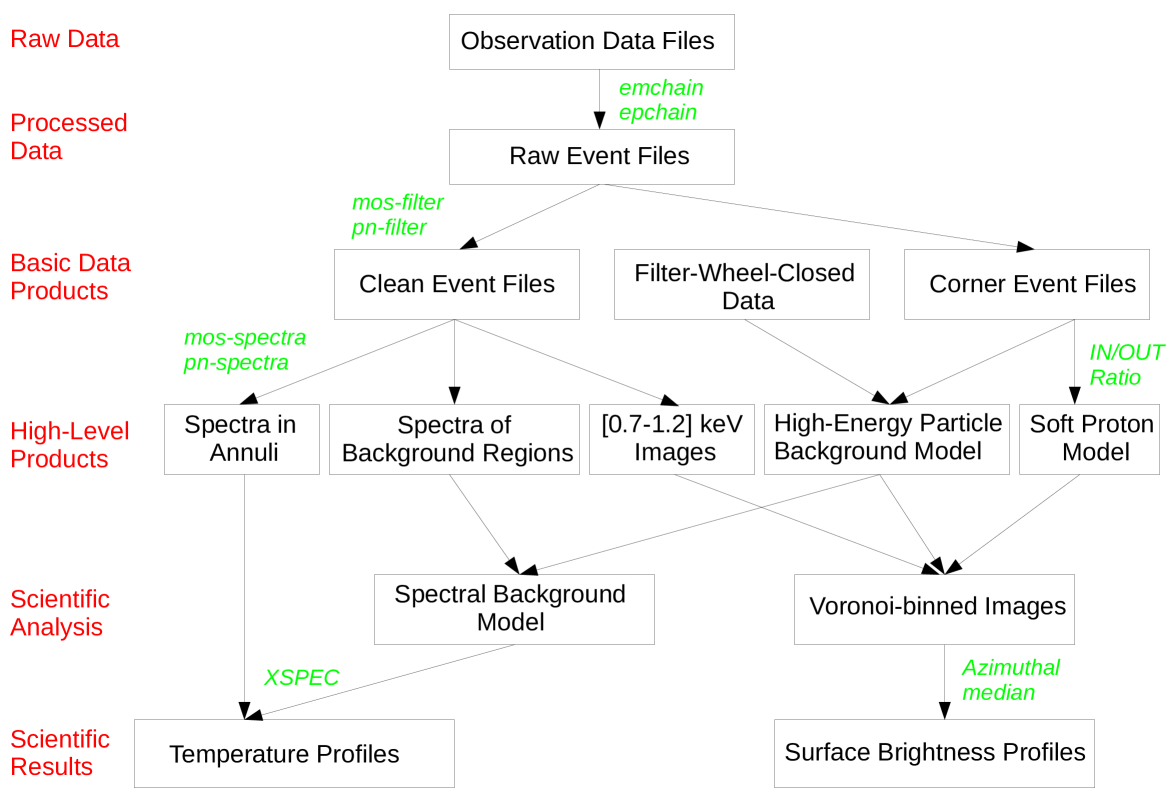
Here we describe in detail the data analysis pipeline that we set up for the analysis of the XMM-Newton data. A flow chart describing the main steps of the analysis is presented in Fig. 1.

Figure 1: Flow chart of the XMM-Newton data analysis pipeline. The steps of the analysis are shown in red, the main intermediate and final products are described in the black boxes, and the procedures are shown in green italics.

2.2.1 Data reduction

We reduced all the data using XMMSAS v13.5 and the Extended Source Analysis Software (ESAS) data reduction scheme (Snowden et al., 2008). To perform basic data reduction, we used the emchain and epchain pipelines to extract calibrated event files from the observations, and we reran epchain in out-of-time mode to create event files for pn out-of-time events. To filter out time periods affected by soft proton flares we ran the mos-filter and pn-filter executables, which extract the light curve of each observation in the hard band, and applied a sigma-clipping technique to exclude time intervals with enhanced background. We used the unexposed corners of the MOS detectors to monitor the particle background level during each observation, and measured the count rates in the high-energy band ([7.5-11.8] keV) of the MOS from the regions located inside and outside the field of view (FOV) of the telescope (hereafter IN and OUT). The comparison between IN and OUT count rates was then used to estimate the contamination of residual soft protons to the spectrum (De Luca & Molendi, 2004; Leccardi & Molendi, 2008; Salvetti et al., 2017).

2.2.2 Image extraction and preparation

We extracted photon count images from the three EPIC detectors in the [0.7-1.2] keV band. This narrow band maximizes the ratio between source and background emission and is thus best suited to minimize the systematics in the subtraction of the EPIC background (Ettori et al., 2010). We used eexpmap to compute exposure maps taking vignetting effects into account for all three detectors independently. To create total EPIC images, we summed the count maps of the three detectors and repeated the same operation with the exposure maps, multiplying the pn exposure maps by a factor of 3.44 representing the ratio of pn to MOS effective areas in our band of interest. The high-energy particle background are modeled and subtracted by simple subtraction of the rescaled background images, taken from the unexposed corners of the detectors.

Even after cleaning the light curves from soft-proton flares, it is known that a fraction of residual soft proton contamination remains within the datasets. This component can introduce systematics at the level of $\sim 20\%$ in the subtraction of the EPIC background in our band of choice (Tchernin et al., 2016). To model the contribution of residual soft protons, we follow the method outlined in Ghirardini et al. (2017), which was calibrated using a large set of $\sim 500$ blank-sky pointings. Namely, we measure the high-energy ([7.5-11.85] keV) MOS count rates in the exposed (IN) and unexposed (OUT) parts of the FOV, and we use the difference between IN and OUT count rates as an indicator of the contamination of each observation by residual soft protons (see Salvetti et al., 2017, for a detailed overview of this approach). We use our large blank field dataset to calibrate an empirical relation between the IN-OUT indicator and the required intensity of the soft proton component (see Appendix A of Ghirardini et al., 2017), and we use this relation to create a 2D soft proton model. This procedure was shown to bring the systematics in the subtraction of the EPIC background to an accuracy better than 5%.

Figure 2: Adaptively smoothed and exposure corrected XMM-Newton mosaic images in the [0.7-1.2] keV energy band for all X-COP clusters. The superimposed white contours represent the Planck SZ S/N maps between 70 and 857 GHz. The contour levels correspond to 1, 3, 5, 7, 10, 15, 20, 30, 40, and 50$\sigma$. The spatial scale is given by the red thick lines, which have a common length of 15 arcmin. The color scale is given below the images in units of cts s^-1 pixel^-1, and is the same for all clusters.

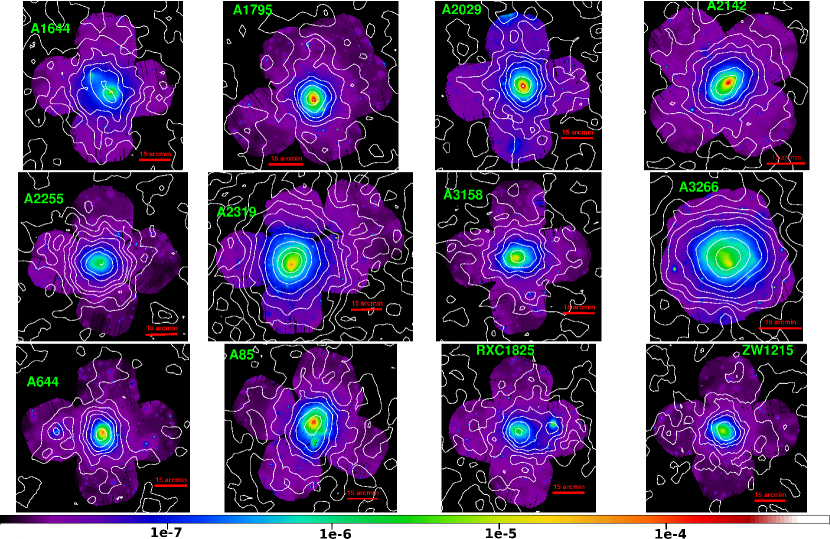
For each cluster, we combine the resulting EPIC count maps in the [0.7-1.2] keV from each individual observation (central or offset) to create a mosaic image. We apply the same procedure to the combined EPIC exposure maps and to the background maps, summing the non-X-ray background components (quiescent particle background and residual soft protons). We then obtain mosaicked photon maps, exposure maps, and non-X-ray background maps for each source. In Fig. 2 we show the resulting background-subtracted and exposure-corrected mosaics, which we adaptively smoothed using the asmooth code (Ebeling et al., 2006).

2.2.3 Point source subtraction

To detect point sources present within the field, we extract photon count maps from the three detectors in a soft ([0.5-2] keV) and a hard ([2-7] keV) band, and we use the XMMSAS tool ewavelet with wavelet scales in the range 1–8 pixels and signal-to-noise ratio threshold of 5.0. We then cross-match the soft and hard band detections between the multiple (central and offset) observations of each cluster to create a global point source list per cluster. Since the vignetting and the point spread function of the XMM-Newton telescopes depend on off-axis angle, the sensitivity threshold for source detection depends on the position of a source on the detector. At a fixed observing time, XMM-Newton thus detects point sources down to lower fluxes near the aim point than close to the edge of the FOV, and the fraction of the cosmic X-ray background (CXB) that is resolved by the instrument is spatially dependent. To correct for this effect, we draw the distribution of measured count rates from the detected sources and we determine the count rate at which the distribution peaks. Since the logN-logS of distant sources contributing to the CXB is a monotonically decreasing function (e.g., Moretti et al., 2003) the peak in the count rate distribution of our observation roughly corresponds to the threshold down to which our source detection is complete. We then excise only the sources with a measured count rate greater than our threshold and leave the fainter sources to enforce a constant flux threshold across the FOV and avoid biasing local measurements of the CXB intensity.

2.2.4 Surface brightness profiles

An important complication with the analysis of X-ray data of cluster outskirts lies in the presence of accreting structures and inhomogeneities in the gas distribution, which are expected to contribute substantially to the measured X-ray flux beyond $\sim R_{500}$ (e.g., Nagai & Lau, 2011; Vazza et al., 2013; Roncarelli et al., 2013). Since the X-ray emissivity is proportional to the square of the gas density, overdense regions contribute predominantly to the measured X-ray flux and can bias high the recovered gas density. To avoid this problem we apply the azimuthal median method outlined in Eckert et al. (2015). Numerical simulations show that the median surface brightness in concentric annuli is robust against the presence of outliers in the gas density distribution (Zhuravleva et al., 2013). We thus construct background-subtracted and exposure-corrected surface brightness maps using a Voronoi tessellation technique (Cappellari & Copin, 2003) with a target number of 20 counts per bin.

The intensity of the sky background is determined by averaging the surface brightness distribution in the regions with $R>2R_{500}$, where we assume the cluster emission to be negligible. A systematic uncertainty of 5% of the background level (see Sect. 2.2.2) was added in quadrature to the error budget of the surface brightness profiles. This procedure was applied to all clusters except A3266, for which the current mosaic does not extend out to $2R_{500}$. In this case, we estimate the sky background intensity from the ROSAT all-sky survey background tool and included a systematic error of 30% in quadrature to the full error budget.

To compute the surface brightness profiles, we draw the surface brightness distribution from the Voronoi-binned images in concentric radial bins starting from the X-ray peak and then choosing the annuli such that the emissivity in each bin is almost constant. The errors on the azimuthal median are estimated from $10^{4}$ bootstrap resampling of the pixel distribution. Circular regions of 30 arcsec radius are excised around the positions of point sources selected through the procedure described in Sect. 2.2.3, corresponding to an encircled energy fraction of 90% of the point source flux.

2.3 Deprojection and gas density profiles

To extract gas density profiles, we take advantage of the fact that the X-ray surface brightness in our energy band of choice is proportional to the squared gas density integrated along the line of sight. To convert surface brightness profiles into emission measure, we describe the emissivity of the source with a thin-plasma model absorbed by the Galactic $N_{H}$ and folded through the on-axis EPIC/MOS effective area. This approach allows us to calculate the conversion between the observed count rate in MOS units and the normalization of the APEC model, which is related to the plasma emission measure as

$$\mbox{Norm}=\frac{10^{-14}}{4\pi[d_{A}(1+z)]^{2}}\int_{V}n_{e}n_{H}\,dV,$$ (1)

where $d_{A}$ is the angular diameter distance of the source, and $n_{e}$ and $n_{H}$ are the electron and ion number densities in units of cm^-3, with $n_{e}=1.17n_{H}$ in a fully ionized plasma (Anders & Grevesse, 1989). Since we are using a soft energy band, the conversion between count rate and emission measure shows little dependence on the temperature as long as the temperature exceeds $\sim 1.5$ keV, which is the case in all X-COP systems. The resulting emission measure profiles can then be deprojected under the assumption of spherical symmetry by computing the projected volumes V of each spherical shell onto each 2D annulus. To recover the 3D emissivity and density profiles from the projected data, we apply two different deprojection methods that we briefly outline here.

• L1 regularization: This method builds on the non-parametric regularization approaches developed by Croston et al. (2006) and Ameglio et al. (2007), introducing a penalty term on the modulus of the second derivative of the 3D density profile to kill spurious small-scale fluctuations introduced by the random nature of the data (Diaz-Rodriguez et al., 2017). Given an observed 2D emission measure profile ${EM=(EM_{1}\dots EM_{n}})$ and corresponding uncertainties ${\sigma_{EM}=(\sigma_{EM,1}\dots\sigma_{EM,n}})$ , the values of the 3D emissivity profile ${\epsilon=(\epsilon_{1}\dots\epsilon_{n}})$ are obtained by maximizing the following likelihood function

  $$-2\log\mathcal{L}=\chi^{2}=\sum\frac{(V\#\epsilon-EM)^{2}}{\sigma_{EM}^{2}}+\lambda\sum\left|\frac{\partial^{2}\log\epsilon}{\partial\log r^{2}}\right|,$$ (2)

  where $V_{i,j}$ is the geometrical matrix volume of the jth shell intercepted by the ith annulus, $\#$ is the symbol for matrix product, and the sum is performed along all the annuli. Moreover the second derivative of the emissivity is computed as a numerical derivative of the $\epsilon(r)$ vector. The parameter $\lambda$ controls the degree of regularization of the profile. To maximize the likelihood function described in Eq. 2, we use the Markov chain Monte Carlo (MCMC) tool emcee (Foreman-Mackey et al., 2013), leaving the value of the 3D density profile at each radius as a free parameter and setting a logarithmic prior (i.e., uniform prior in logarithmic space) on each parameter value to enforce positivity of the resulting profile. The value of the parameter $\lambda$ is chosen such that the log-likelihood is about 1 per data point, to allow for typical statistical deviations of $1\sigma$. We note that $\lambda=0$ is equivalent to using the onion-peeling technique directly (see Kriss et al., 1983; Ettori et al., 2002, 2010).

• Multiscale fitting: This method follows the technique developed in Eckert et al. (2016), whereby the projected emission measure profile is decomposed into a sum of analytical multiscale functions which can be individually deprojected. Following Eckert et al. (2016) we write the observed 2D profile as a sum of $N$ King functions with fixed core radii and normalizations and slopes allowed to vary while fitting, choosing $N=N_{points}/4$; i.e., one model component is added for every set of four data points, fixing a core radius to the mean radial value of these four data points. Since the projection kernel is linear, each King function can be individually deprojected and the 3D profile can be analytically reconstructed from the fit to the projected data. As above, we use emcee to optimize for the parameters and reconstruct the error envelope around the best fitting curve.

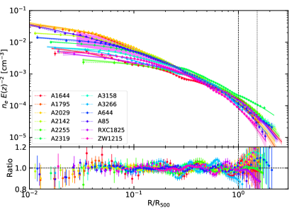
In the top left panel of Fig. 3 we compare the density profiles reconstructed with the two methods and find a remarkable agreement between them, with an average scatter $<5\%$ at each radius. By construction, the profiles reconstructed with the L1 regularization method shows more pronounced features as the method imposes fewer constraints on the shape of the profile, whereas the profiles obtained with the multiscale method are smoother. Thus, we adopt the results of the L1 regularization when attempting to determine the exact shape of our profiles, whereas the multiscale technique is preferred when reconstructing hydrostatic mass profiles to provide better control over the gradient.

2.4 Spectral analysis

2.4.1 Spectral extraction

We extract spectra in concentric annuli around the X-ray peak covering approximately the radial range $[0-1]R_{500}$, removing the point sources which contaminates the spectra (see Sec. 2.2.3). In the spectral analysis, differently from the imaging case in Sect. 2.2.2, we compute models of the high-energy particle background using the ESAS tools mos-spectra and pn-spectra in imaging mode. To this end, we select the filter-wheel-closed observations recorded at the nearest possible time to the observation, and we use the spectra of the unexposed corners of the detectors to rescale the filter-wheel-closed observations. This procedure is performed individually for all CCDs, and the CCDs operating in anomalous mode are discarded. We then extract an image from the rescaled filter-wheel-closed data in the [0.7-1.2] keV band using the mos-back and pn-back executables, which we use as our model for the high-energy particle background. In the case of the pn, we repeat the operation with the out-of-time event files and create a model for the intensity and spatial distribution of out-of-time events.

We selected the binning such that the width of the bins increases exponentially, but choosing a minimum width of 0.5 arcmin for the innermost bins such that the instrumental PSF does not contribute much to the photon in each bin. We group the output spectra with a minimum of five counts per bin to ensure stable fitting results, and discard the data below 0.5 keV where the EPIC calibration is uncertain. We then use Xspec v12.9 and the C-statistic (Cash, 1979) to fit the spectra and determine the plasma parameters (see Sect. 2.4.2).

2.4.2 Spectral modeling

To extract spectral diagnostics from the observed spectra (see Sect. 2.4.1), we proceeded using a full spectral modeling approach following the method described in detail in Eckert et al. (2014). Here we describe our approach to model all the individual background components and the source spectra.

• High-energy particle background : We use the rescaled filter-wheel-closed spectra to determine the intensity and spectral shape of the particle background. We fit the filter-wheel-closed spectra using a diagonal response matrix and a phenomenological model including a broken power law and several Gaussians to reproduce the shape of the continuum and fluorescence lines. We then apply the fitted model to the source spectrum, leaving the normalization free to vary within $\pm 10\%$ to account for possible systematics in the scaling of the filter-wheel-closed data.

• Sky background : We model the X-ray background and foreground emission as the sum of three components: i) an absorbed power law with a photon index fixed to 1.46 to describe the residual CXB (De Luca & Molendi, 2004); ii) an absorbed APEC thermal plasma model with a temperature allowed to vary in the range [0.15-0.6] keV to model the Galactic halo emission (McCammon et al., 2002); and iii) an unabsorbed APEC model with a temperature fixed to 0.11 keV to represent the local hot bubble. The Galactic hydrogen column density $N_{H}$ was fixed to the LAB value (Kalberla et al., 2005). Similarly to what was done for the imaging case, the parameters of the sky emission model are fitted to the spectra of background regions located at $R>2R_{500}$ from the cluster core. Again the exception to this procedure is A3266, for which we use the ROSAT all-sky survey background tool to determine the sky background parameters. The best fit model is then applied to the source spectra, rescaling the intensity of the components according to the area of each region.

• Residual soft protons : In cases where our IN-OUT indicator of soft proton contamination is found to be high (IN-OUT¿0.1 counts/s), we include an additional model component to the particle background model to take soft protons into account. We model the soft proton component as a broken power law with fixed spectral shape (slopes 0.4 and 0.8 and break energy 5 keV, Leccardi & Molendi, 2008) and leave the normalization of this component free to vary in the overall fitting procedure.

• Source : We model the source emission in each annulus as an absorbed single-temperature APEC model with temperature, emission measure, and metal abundance free to vary. In cases where multiple observations were available for the same regions, we fit all the available spectra jointly, tying the source parameters between the different spectra. The solar abundance table is set to Anders & Grevesse (1989). Since our objects are nearby and extended on scales much larger than the XMM-Newton PSF, we neglect the potential cross-talk between the various annuli.

All the spectra were fitted in the energy range [0.5-12] keV using Xspec v12.9, ATOMDB v3.0.7, and the C-statistic (Cash, 1979). When several observations of the same region were available, we extracted the spectra from each individual pointing and fit them jointly. We ignored the energy ranges [1.2-1.9] keV (MOS) and [1.2-1.7] keV, [7.0-9.2] keV (pn) where bright and time-variable fluorescence lines were present. We then constructed projected gas temperature profiles from the best fit results. We also deprojected our 2D temperature profiles using the projection matrix V and the emissivity in each annulus as weights, adopting the spectroscopic-like temperature scaling of Mazzotta et al. (2004).

2.5 Planck data analysis

The signal was recovered from the Planck survey (Tauber et al., 2010; Planck Collaboration et al., 2016a) making use of the six frequency maps provided by the High Frequency Instrument (HFI Lamarre et al., 2010; Planck HFI Core Team et al., 2011). They were combined with a modified internal linear combination algorithm (MILCA, Hurier et al., 2013) to produce Comptonization parameter maps, i.e., $y$-maps tracing the intensity of the SZ effect. The maps used for the X-COP project are provided with a resolution of 7 arcmin FWHM.

The intra-cluster gas thermal pressure integrated is recovered from the $y$ parameter (Sunyaev & Zeldovich, 1972) as

$$y(\theta)=\frac{\sigma_{T}}{m_{e}c^{2}}\int P(\ell)d\ell,$$ (3)

where the integral is computed along the line of sight, $\theta$ is the angular distance to the cluster core, $\sigma_{T}$ is the Thomson cross-section, $m_{e}$ is the mass of the electron, and $c$ is the speed of light.

As illustrated for the cases of A2142 (Tchernin et al., 2016) and A2319 (Ghirardini et al., 2017), we followed for the whole X-COP sample the methodology presented and used in Planck Collaboration et al. (2013). Assuming azimuthal symmetry of the cluster, we computed the $y$ radial profile for each cluster over a regular grid scaled in units of $R_{500}$ with radial bins of size $\Delta\theta/\theta_{500}=0.2$ out to $10\times R_{500}$. The local background is assumed to be flat and constant and is computed from the area beyond $5\times\theta_{500}$. A covariance matrix is computed for each profile to account for the correlation between points due to the profile binning, and intrinsic noise correlation introduced from the $y$ map construction.

We corrected from the Planck beam redistribution through a real space deconvolution of the instrument PSF. Further assuming the spherical symmetry of the source, we reconstructed each pressure profile through a geometrical deprojection. The two steps follow the method initially presented in Croston et al. (2006). The associated covariance matrix for the pressure profile is obtained via a Monte Carlo procedure by randomizing over the initial $y$ profile covariance matrix. In the following we ignore the innermost three Planck data points because of the difficulty deconvolving from the large Planck beam.

As an alternative method, we also extracted Planck pressure profiles using the forward-modeling approach of Bourdin et al. (2017). In this case, a spectral model for the relevant components is constructed (CMB, dust, synchrotron, and thermal SZ). The model is folded through the Planck response and fitted to the multi-frequency data points (see Bourdin et al., 2017, for details). In Appendix B we compare the results obtained with this approach to the results of the MILCA component separation method and show their consistency. For the remainder of the paper, we use the MILCA pressure profiles as our default choice.

Figure 3: Top left panel: Density profiles for all X-COP clusters obtained with two different deprojection methods: L1 regularization (data points) and multiscale fitting (solid lines). The magenta shaded area represents the scatter of the median profile in Eckert et al. (2012). The bottom panel represents the ratio of the two methods for each individual system. Top right panel: Joint fit to all the density profiles using piecewise power laws in several radial ranges (color-coded). The best fits and $1\sigma$ error envelope are shown by the solid lines, while the dashed lines represent the intrinsic scatter. Bottom left panel: Joint fit to the density profiles using the functional form introduced by Vikhlinin et al. (2006), in red, with the shaded area indicating the 1$\sigma$ error envelope around the best fit. The dashed lines represent the intrinsic scatter in the functional form as a function of radius. Bottom right panel: Slope of the density profiles as a function of radius. The green data points show the results of the piecewise power law fits, whereas the red curve indicates the fit to the entire radial range using the Vikhlinin et al. (2006) functional form. In all panels, the vertical dashed and dotted lines represent the location of $R_{500}$ and $R_{200}$, respectively.

Figure 4: Same as Fig. 3 for the pressure profiles rescaled by the self-similar quantity $P_{500}$ (Eq. 8). The squares indicate data points obtained from the deprojection of the SZ signal, while the filled circles are computed by combining the X-ray gas density profiles with the spectroscopic temperature. The solid red curve in the bottom panels shows the joint best fit to the data with the generalized NFW functional form (Nagai et al., 2007, see Eq. 9). In all these plots the dotted and dashed-dotted lines represent the result of Planck Collaboration et al. (2013) and Arnaud et al. (2010) respectively. The shadow areas represent the envelope obtained by Planck Collaboration et al. (2013) and the Early release SZ sample(XMM-ESZ, Planck Collaboration et al., 2011).

Figure 5: Same as Fig. 3 for the projected temperature profiles rescaled by the self-similar quantity $T_{500}$ (Eq. 10). The filled circles show the measurements of the X-ray spectroscopic temperature (see Sect. 2.4.2), whereas the filled squares indicate the data points obtained by combining the SZ pressure with the gas density, projected along the line of sight assuming the spectroscopic-like scaling of Mazzotta et al. (2004). The solid red curves in the bottom panels show the best fit to the joint dataset with the functional form introduced by Vikhlinin et al. (2006) (see Eq. 11).

Figure 6: Same as Fig. 3 for the entropy profiles rescaled by the self-similar quantity $K_{500}$ (Eq. 12). The filled circles show the measurements obtained from the X-ray spectroscopic temperature as $K=k_{B}T/n_{e}^{2/3}$, whereas the filled squares indicate the data points obtained by combining the SZ pressure with the gas density as $K=P_{e}/n_{e}^{5/3}$. The solid red curves in the bottom panels indicate the best fit to the entire population with the functional form presented in Eq. 13, whereas the solid black line shows the prediction of pure gravitational collapse (Voit et al., 2005).

2.6 Mass estimates

To estimate scale radii and self-similar scaling quantities, we use the high-precision hydrostatic mass reconstructions presented in Ettori et al. (2018). The mass models were obtained by combining X-ray and SZ information for each individual system and solving the hydrostatic equilibrium equation. For the present work, we adopt as our reference mass model the backward NFW results, which were obtained by assuming that the mass profile follows a Navarro-Frenk-White shape (Navarro et al., 1996) with scale radius and concentration $c_{200}$ as free parameters. This method was shown to provide the best representation of the data (Ettori et al. 2018) and at $R_{500}$ it matches the results obtained without assuming a functional form for the mass profile with an accuracy of $\sim 5\%$. Comparison of our mass reconstruction with weak lensing and SZ estimates (Ettori et al. 2018) and convergence toward the expected universal gas fraction (Eckert et al. 2018) show that our masses and the corresponding values of $R_{500}$ are accurate at the $10\%$ and $3\%$ level, respectively. For more details on the reconstruction of hydrostatic masses and estimates of systematic uncertainties we refer to Ettori et al. (2018) and Eckert et al. (2018).

3 Thermodynamic properties

In the following section we describe how we derived the universal profiles, slopes, and intrinsic scatter of all our thermodynamic variables. We then present our main results and provide best fitting functional forms describing the X-COP cluster population.

3.1 Fitting procedure

We adopt two different approaches to fit the thermodynamic properties:

• Piecewise power law fits: In this case, we split our data into several radial ranges as a fraction of $R_{500}$ and we approximate the global behavior of the population in each range as a power law with free log-normal intrinsic scatter

  $$\frac{Q(x)}{Q_{500}}=A\cdot x^{B}\cdot\exp(\pm\sigma_{\rm int})$$ (4)

  with $x=R/R_{500}$; $Q/Q_{500}$ the rescaled thermodynamic quantity at an overdensity of 500; and $A$, $B$, and $\sigma_{\rm int}$ the normalization, slope, and intrinsic scatter in the radial range of interest. The values of $Q_{500}$ are computed adopting the virial theorem as in Voit et al. (2005), and are shown in Eq. (8), (10), and (12). The fitting procedure thus has three free parameters ($A$, $B$, and $\sigma_{\rm int}$) in each of the chosen radial ranges. We note that this procedure provides model independent measurements of the slope and intrinsic scatter at different radii.

• Global functional forms: In this case, we describe the radial dependence of the thermodynamic quantity of interest throughout the entire radial range with a parametric functional form found in the literature

  $$\frac{Q(x)}{Q_{500}}=f(x)\cdot\exp\left[\pm\sigma_{\rm int}(x)\right]$$ (5)

  with $Q/Q_{500}$ the rescaled thermodynamic quantity at an overdensity of 500, as in Eq. (4), and $f(x)$ the chosen functional form for the thermodynamic quantity $Q$. In this case, since we model the whole radial range covered by our measurements, we allow the intrinsic scatter to vary with radius following a quadratic functional form to model the radial dependence of the intrinsic scatter

  $$\sigma_{\rm int}(x)=\sigma_{1}\log^{2}\left(\frac{x}{x_{0}}\right)+\sigma_{0}$$ (6)

  with $\sigma_{1}$ the width of the log-parabola, and $x_{0}$ and $\sigma_{0}$ respectively the location and the intercept of the minimum of the log-parabola. A total of $n+3$ parameters are allowed to vary during the fitting procedure, with $n$ the number of parameters of the adopted functional form $f(x)$. Optimizing jointly for the parameters of the intrinsic scatter profile allows us to determine the shape of $\sigma_{\rm int}(x)$.

In Figs.  3– 6 we show our rescaled thermodynamic quantities for the gas density, pressure, temperature, and entropy. The best fits with piecewise power laws and using functional forms are presented as well, together with the slopes for the parametric and non-parametric cases.

3.2 Density

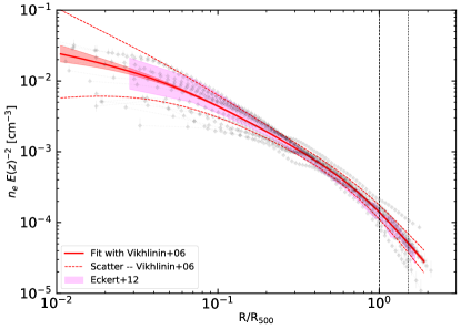
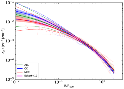
We rescaled our density profiles by the self similar quantities, $E^{2}(z)=\Omega_{m}(1+z)^{3}+\Omega_{\Lambda}$ and $R_{500}$ for density and radius, respectively. In Fig. 3 we compare our scaled gas density profiles with the “universal” density profiles from Eckert et al. (2012) from a sample of 31 clusters with available ROSAT/PSPC pointed data. We observe excellent agreement with their results; A2319 is the only exception that deviates at large radii, as shown in Ghirardini et al. (2017), because of its large non-thermal pressure support.

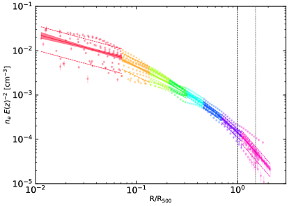
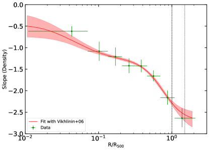
In the top right panel of Fig. 3 we show our density profiles fitted with piecewise power laws in several radial ranges, we show the best fitting parameters in Table 2. We parametrize the behavior of our density profiles over the whole radial range by adopting the Vikhlinin et al. (2006) functional form

$$f^{2}(x)=n_{e}^{2}(x)=n_{0}^{2}\frac{(x/r_{c})^{-\alpha}}{(1+x^{2}/r_{c}^{2})^{3\beta-\alpha/2}}\frac{1}{(1+x^{\gamma}/r_{s}^{\gamma})^{\epsilon/\gamma}}$$ (7)

with $x=R/R_{500}$ and $\gamma=3$ fixed. The form thus has six free parameters ($n_{0}$, $r_{c}$, $\alpha$, $\beta$, $r_{s}$, and $\epsilon$) and is able to reproduce both the core and the outer parts of the density profile. We apply flat priors in logarithmic space to $n_{0}$, $r_{c}$, and $r_{s}$ and flat priors in linear space to the remaining parameters, constraining $\epsilon<5$ (we specify the priors adopted in Table 3). We show the posterior distributions of the parameters of this functional form in Fig. 14 and the covariance between them.

The resulting profile is consistent at all radii with the universal envelope computed by Eckert et al. (2012). We can see in all panels how the profiles become progressively less scattered going toward the outskirts. While the core is affected by a large scatter likely caused by cooling, AGN feedback and different merger states, the profiles show a high degree of self-similarity in the radial range $[0.3-1]R_{500}$. Then in the outskirts the scatter increases again, likely caused by different accretion rates from one system to another. We note from the plot in bottom right panel in Fig. 3 that the slope of the density profiles steepens steadily with radius. The slopes computed from the piecewise power law fits and from the global fit with Eq. 7 agree within 1$\sigma$ at all points. Again, this result agrees with the findings of Eckert et al. (2012) and Morandi et al. (2015), but is at variance with the relatively flat slopes reported in several clusters observed by Suzaku. For instance, several papers report density slopes flatter than $-2.0$, for example $-1.7$ in the outskirts of the Perseus cluster (Urban et al., 2014) or even as low as $-1.2$ in A1689 (Kawaharada et al., 2010) and Virgo (Simionescu et al., 2017). These measurements are clearly in tension with the slope of $-2.5$ at $R_{200}$ measured here for the X-COP cluster population. It must be noted, however, that thanks to the azimuthal median technique, our gas density profiles are essentially free of the clumping effect, whereas the Suzaku studies could not properly excise overdense regions because of the lower resolution of the instrument and/or observations performed along narrow arms.

3.3 Pressure

Pressure in galaxy clusters is usually the smoothest thermodynamic quantity along the azimuth, if the cluster is not affected by an ongoing merger.

We recover the gas pressure both through the combination of X-ray gas density and spectral temperature and through the direct deprojection of the SZ effect. In the former case, we deproject the spectral X-ray temperature (e.g., Mazzotta et al., 2004, see Sect. 2.4.2) and combine the deprojected temperature with the gas density interpolated on the same grid to infer the pressure $P_{X}=k_{B}T_{X}\times n_{e}$. In the latter we recover the pressure directly from the Planck data by deprojecting the measured $y$ profiles (see Sect. 2.5) from which we exclude the first three points from the analysis. We thus combine the higher resolution and precision of XMM-Newton in the inner region with the high quality of the Planck data at $R_{500}$ and beyond, which allows us to constrain the shape and intrinsic scatter of the pressure profiles in the radial range $[0.01-2.5]R_{500}$. We rescale our pressure profiles by the self-similar quantities at an overdensity of 500,

$$P_{500}=3.426\times 10^{-3}\text{\ keV}\text{\ cm}^{-3}\left(\frac{M_{500}}{h_{70}^{-1}10^{15}M_{\odot}}\right)^{2/3}E(z)^{8/3}\cdot\\ \cdot\left(\frac{f_{b}}{0.16}\right)\left(\frac{\mu}{0.6}\right)\left(\frac{\mu_{e}}{1.14}\right),$$ (8)

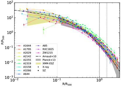
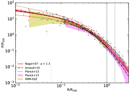
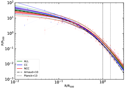
where $f_{b}$ is the Universal gas fraction, which we take to be $\Omega_{b}/\Omega_{m}=0.16$ (Planck Collaboration et al., 2016c, rounding the number to 2 significant figures), $\mu$ and $\mu_{e}$ are the mean molecular weight per particle and mean molecular weight per electron for which we adopt the values measured by Anders & Grevesse (1989). In Fig. 4 we show the scaled pressure profiles of our 12 objects obtained through X-ray and SZ measurements of the ICM. We note that our profiles agree with the results obtained by the Planck Collaboration for a sample of 62 clusters (Planck Collaboration et al., 2013), falling well within the two envelopes, with the exception, as in the case of the density, of A2319 (see the discussion in Ghirardini et al., 2017).

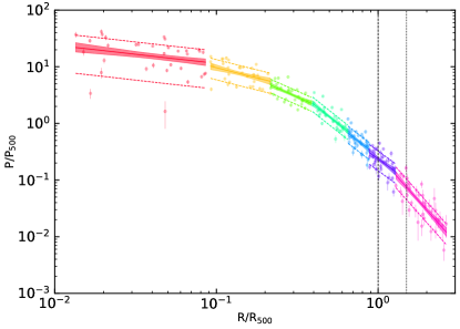
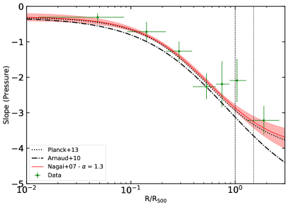
Similarly to the density, we fitted the profiles using piecewise power laws in several radial ranges, also obtaining in this case a scatter that decreases with radius out to $R_{500}$ and then (as for the density) that increases in the outskirts; these profiles become progressively steeper with radius, see Table 2. Our profiles in the outskirts are compatible with the results of the Planck Collaboration, both for the central value and the slope. We also fitted our data using the generalized NFW functional form introduced by Nagai et al. (2007)

$$f(x)=\frac{P(x)}{P_{500}}=\frac{P_{0}}{(c_{500}x)^{\gamma}[1+(c_{500}x)^{\alpha}]^{\frac{\beta-\gamma}{\alpha}}},$$ (9)

where $x=R/R_{500}$, with five free parameters $P_{0}$, $c_{500}$, and three slopes, $\gamma$, $\alpha$, and $\beta$ representing respectively the inner, intermediate, and outer slopes (we specify the priors adopted in Table 3). Since the parameters are strongly degenerate, it was advised to fix at least one of the slopes (Arnaud et al., 2010); therefore, we fixed the central slope $\alpha$ to the best fit value of 1.3 estimated by the Planck Collaboration (Planck Collaboration et al., 2013). The resulting best fit, the intrinsic scatter around the median profile, and the slope computed from the fit are shown in Fig. 4. The posterior distributions of the parameters and the covariance between them are shown in Fig. 15.

Similar to the case of the gas density, we find that the slope of the profiles steepens steadily with radius, as expected for a gas in hydrostatic equilibrium within a NFW potential. The best fit with the generalized NFW functional form does an excellent job of reproducing the slopes estimated from the piecewise power law fits.

In the range where pressure measurements are available both from XMM-Newton and Planck, we find excellent agreement between the two (see Appendix A) even though the pressure profiles were obtained using completely independent probes. This shows that X-ray and SZ observations provide a consistent picture of the state of the ICM and gives us confidence that systematics in our measurements are small and under control.

3.4 Temperature

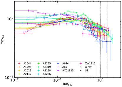
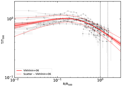
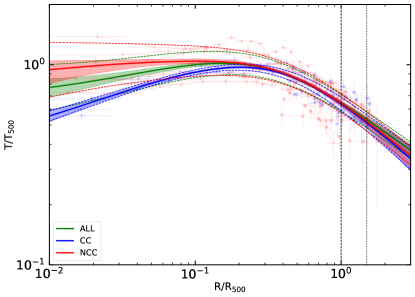
Temperature profiles in X-ray studies are usually obtained by performing spectral fitting in concentric annuli (see Sect. 2.4.2), called the spectroscopic temperature. In addition, we also use our Planck SZ pressure profiles and combine them with the X-ray density profiles to obtain gas-mass-weighted temperatures $T_{gmw}=P_{SZ}/n_{e}$, which are then projected (using the X-ray emissivity as weight, as in Mazzotta et al., 2004) on the plane of the sky and overplotted on the spectroscopic temperatures. Our X-ray and SZ measurements of pressure and temperature cover different radial ranges. X-ray spectroscopy probes the temperature of the gas within $R_{500}$, while SZ probes temperatures from $0.7R_{500}$ to $2R_{500}$ (excluding the first three SZ data points), which highlights the complementarity of the two ICM diagnostics. In Fig. 5 we show our 2D spectral temperature profiles rescaled by $T_{500}$, defined as

$$T_{500}=8.85\text{\ keV}\left(\frac{M_{500}}{h_{70}^{-1}10^{15}M_{\odot}}\right)^{2/3}E(z)^{2/3}\left(\frac{\mu}{0.6}\right)$$ (10)

While density and pressure change by three to four orders of magnitude going from the center to the outskirts of the cluster, temperature shows much milder variations. In particular, it is almost constant out to $\sim 0.5R_{500}$, and then declines beyond this point.

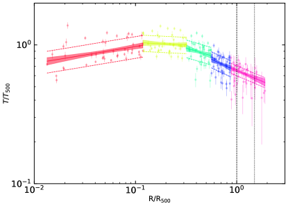
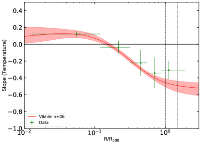
In Fig. 5 we show the results of the piecewise power law fits in several radial ranges. We perform a global fit to the temperature profiles with the functional form described in Vikhlinin et al. (2006), which is able to describe the temperature profiles of both the core and the outer parts of galaxy clusters

$$f(x)=\frac{T(x)}{T_{500}}=T_{0}\frac{\frac{T_{min}}{T_{0}}+\left(\frac{x}{r_{cool}}\right)^{a_{cool}}}{1+\left(\frac{x}{r_{cool}}\right)^{a_{cool}}}\frac{1}{\left(1+\left(\frac{x}{r_{t}}\right)^{2}\right)^{\frac{c}{2}}}$$ (11)

with $x=R/R_{500}$, and six free parameters: $T_{0}$, $T_{min}$, $r_{cool}$, $a_{cool}$, $r_{t}$, and $c$ (we specify the priors adopted in Table 3). The posterior distribution of these parameters and the covariances are shown in Fig. 16. This functional form provides an accurate description of the shape of the temperature profiles. The slopes estimated from the global fit follow the slopes measured from the piecewise power law fits at different radial ranges within $1\sigma$ at every radius.

The average slope of the temperature profiles is slightly positive in the central regions because of effects due to cooling, especially in cool-core clusters. Beyond $\sim 0.5R_{500}$ the slope remains relatively flat at a value of $-0.3$. This value is consistent with the slopes measured inside $R_{500}$ from XMM-Newton and Chandra data (Leccardi & Molendi, 2008; Pratt et al., 2007), but it is flatter than the typical slopes measured in Suzaku data. From a collection of a dozen clusters with published Suzaku temperature profiles, Reiprich et al. (2013) report that the universal shape of the profiles can be well described by the form $T/\langle T\rangle=1.19-0.84(R/R_{200})$, i.e., the data are consistent with a slope of -1.0 in the outskirts, which is much steeper than the results presented here. Again, the low angular resolution of Suzaku may have prevented the authors from removing cool, overdense regions that could bias low the measured spectroscopic temperature. On the other hand, SZ pressure profiles are much less sensitive to gas clumping (e.g., Khedekar et al., 2013; Roncarelli et al., 2013) and our density profiles were corrected for the statistical effect of gas clumping (see Sect. 2.2.2), thus our X/SZ temperatures are closer to gas-mass-weighted temperatures (see the discussion in Adam et al., 2017).

3.5 Entropy

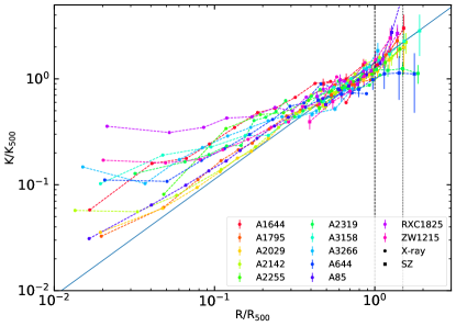
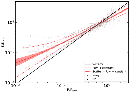
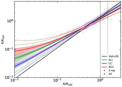
Entropy traces the thermal evolution of the ICM plasma, which can be altered via cooling/heating, mixing, and convection. Simulations predict that in the presence of non-radiative processes only, entropy increases steadily with radius out to $\sim 2\times R_{200}$, following a power law with a slope of 1.1 (Tozzi & Norman, 2001; Voit et al., 2005; Borgani et al., 2005; Lau et al., 2015). The entropy profiles of the cluster population should scale self-similarly when rescaled by the quantity

$$K_{500}=1667\text{\ keV cm}^{2}\left(\frac{M_{500}}{h_{70}^{-1}10^{15}M_{\odot}}\right)^{2/3}E(z)^{-2/3}\cdot\\ \cdot\left(\frac{f_{b}}{0.16}\right)^{-2/3}\left(\frac{\mu}{0.6}\right)\left(\frac{\mu_{e}}{1.14}\right)^{2/3}$$ (12)

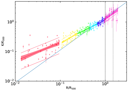
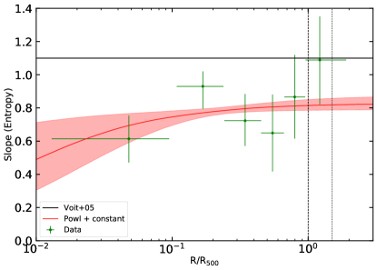
Similarly to pressure and temperature, entropy can be recovered from X-ray-only quantities as $K=k_{B}T_{X}\times n_{e}^{-2/3}$ (using the deprojected temperature; see Sect. 2.4.2) or by combining SZ pressure with X-ray density as $K=P_{SZ}\times n_{e}^{-5/3}$ (ignoring the first three Planck points). We show our scaled entropy profiles in Fig. 6. Our profiles very closely match the predicted power law model beyond $0.3R_{500}$, with just A2319 showing a significant flattening not compatible within the error bars. In the central regions our profiles flatten, with non-cool-core clusters flattening more than cool-core clusters, as already noted in numerous studies (e.g., Pratt et al., 2010; Cavagnolo et al., 2009, and references therein).

By fitting the profile using piecewise power laws we observe a gradual steepening of the entropy slope, which becomes consistent with the predictions of gravitational collapse (Voit et al., 2005) beyond $\sim 0.5R_{500}$, i.e., from a slope of $\sim 0.6$ in the core to $\sim 1.1$ in the outskirts. As for the previous cases, we fitted our profiles throughout the entire radial range with the functional form introduced by Cavagnolo et al. (2009), which consists of a power law with a constant entropy floor

$$f(x)=\frac{K(x)}{K_{500}}=K_{0}+K_{1}\cdot x^{\alpha}$$ (13)

with $x=R/R_{500}$, and three free parameters $K_{0},K_{1}$, and $\alpha$ (we specify the priors adopted in Table 3). The posterior distributions of the parameters and the covariances are shown in Fig. 17. We note that this functional form does not provide an accurate description of the data in the outer parts of the profiles where it is not able to follow the observed gradual change in slope throughout the radial range covered. At large radii, the best fitting slope using Eq. 13 reads $\alpha=0.84\pm 0.04$ (see Table 3), whereas the data prefer a slope consistent with the self-similar prediction of 1.1 beyond $0.6R_{500}$ (see Table 2).

Table 2: Results of the piecewise power law fits (normalizations, slopes, and intrinsic scatter; see Eq. 4) for the various thermodynamic quantities in several radial ranges, marked by the inner and outer rescaled radii $x_{in}$ and $x_{out}$. $\rho_{A,B}$ is the correlation coefficient between A and B.

Density $x_{in}$ $x_{out}$ A ($10^{-4}\rm{cm}^{-3}$) B (slope) $\sigma_{int}$ $\rho_{A,B}$ 0.01 0.07 $13.00\pm 3.83$ $-0.48\pm 0.10$ $0.38\pm 0.04$ 0.9884 0.07 0.13 $3.44\pm 1.73$ $-1.04\pm 0.24$ $0.28\pm 0.03$ 0.9969 0.13 0.21 $2.60\pm 0.79$ $-1.21\pm 0.19$ $0.18\pm 0.02$ 0.9974 0.21 0.31 $2.85\pm 0.72$ $-1.16\pm 0.21$ $0.15\pm 0.01$ 0.9963 0.31 0.46 $1.84\pm 0.31$ $-1.60\pm 0.20$ $0.15\pm 0.01$ 0.9938 0.46 0.72 $1.63\pm 0.17$ $-1.80\pm 0.21$ $0.18\pm 0.02$ 0.9767 0.72 1.14 $1.42\pm 0.06$ $-2.38\pm 0.29$ $0.27\pm 0.03$ 0.7102 1.15 2.00 $1.53\pm 0.19$ $-2.47\pm 0.31$ $0.37\pm 0.04$ -0.8783

Pressure $x_{in}$ $x_{out}$ A B (slope) $\sigma_{int}$ $\rho_{A,B}$ 0.01 0.09 $5.75\pm 2.39$ $-0.31\pm 0.13$ $0.65\pm 0.09$ 0.9353 0.09 0.22 $1.84\pm 1.06$ $-0.72\pm 0.28$ $0.39\pm 0.05$ 0.9321 0.22 0.39 $0.68\pm 0.24$ $-1.27\pm 0.28$ $0.27\pm 0.04$ 0.9550 0.39 0.65 $0.27\pm 0.07$ $-2.27\pm 0.36$ $0.29\pm 0.04$ 0.9636 0.65 0.88 $0.26\pm 0.05$ $-2.19\pm 0.65$ $0.34\pm 0.05$ 0.9371 0.89 1.28 $0.24\pm 0.02$ $-2.09\pm 0.61$ $0.38\pm 0.06$ -0.3866 1.29 2.65 $0.27\pm 0.07$ $-3.21\pm 0.40$ $0.40\pm 0.07$ -0.9363

Temperature $x_{in}$ $x_{out}$ A B (slope) $\sigma_{int}$ $\rho_{A,B}$ 0.01 0.12 $1.29\pm 0.16$ $0.12\pm 0.04$ $0.18\pm 0.02$ 0.9713 0.12 0.32 $0.96\pm 0.11$ $-0.04\pm 0.07$ $0.14\pm 0.02$ 0.9804 0.32 0.56 $0.74\pm 0.10$ $-0.22\pm 0.15$ $0.14\pm 0.02$ 0.9789 0.56 0.87 $0.65\pm 0.04$ $-0.34\pm 0.18$ $0.13\pm 0.02$ 0.9388 0.88 1.90 $0.65\pm 0.02$ $-0.31\pm 0.11$ $0.08\pm 0.02$ -0.4798

Entropy $x_{in}$ $x_{out}$ A B (slope) $\sigma_{int}$ $\rho_{A,B}$ 0.01 0.10 $0.82\pm 0.38$ $0.61\pm 0.14$ $0.56\pm 0.07$ 0.9394 0.11 0.24 $1.57\pm 0.32$ $0.93\pm 0.11$ $0.28\pm 0.03$ 0.9665 0.24 0.45 $1.14\pm 0.20$ $0.72\pm 0.16$ $0.16\pm 0.02$ 0.9783 0.45 0.66 $1.11\pm 0.16$ $0.65\pm 0.23$ $0.16\pm 0.02$ 0.9748 0.67 0.95 $1.20\pm 0.08$ $0.87\pm 0.25$ $0.14\pm 0.02$ 0.9057 0.96 1.90 $1.27\pm 0.08$ $1.09\pm 0.27$ $0.21\pm 0.05$ -0.6778

Figure 7: Measured intrinsic scatter of all our thermodynamic quantities, density (red), pressure (green), temperature (blue), and entropy (black). The data points indicate the results of piecewise power law fits on several radial ranges, whereas the dashed lines and shaded areas show the intrinsic scatter described as a log-parabola (Eq. 6) around the best fitting functional forms.

3.6 Scatter

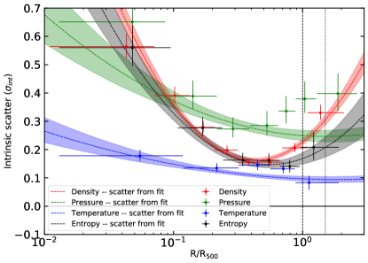
The high data quality of X-COP allows us to probe the intrinsic scatter of our profiles as a function of radius. The piecewise fit using power laws allows us to measure the scatter in a nearly model independent way, whereas the global fit with functional forms and scatter described as a log-parabola provides a consistent description of both the profile shape and the intrinsic scatter throughout the entire radial range. In Fig. 7 we show the scatter of all our thermodynamic quantities obtained in both cases. We recall that our definition of the intrinsic scatter is relative: a value of 0.1 on the $y$-axis indicates that the considered quantity is intrinsically scattered by 10% of its value.

We notice that our thermodynamic profiles generally exhibit a high scatter in the central parts of the profile. The scatter decreases toward the outskirts, reaching a minimum in the range $[0.2-0.8]R_{500}$, and increases slightly beyond this point. We find that temperature is the least scattered thermodynamic quantity, with intrinsic scatters ranging from 10% to 20%. On the contrary, and surprisingly, pressure is the most scattered quantity at all radii (looking at the scatter reconstructed from the piecewise power law fits), ranging from 25% to 60%.

In all cases, we note that our profiles present a high degree of self-similarity in the radial range $[0.2-0.8]R_{500}$, with a typical intrinsic scatter less than 0.3 ($\sim$ 0.1 dex) in all the measured quantities. This radial range corresponds to the region where gravity dominates and baryonic physics (gas cooling, AGN, and supernova feedback) is relatively unimportant, whereas gas accretion still plays a subdominant role. This is consistent with tightly self-regulated mechanical AGN feedback (e.g., via chaotic cold accretion Gaspari et al., 2012), which can only affect the region $<0.1\,R_{500}$, with predicted moderate scatter in T/$n_{e}$ as similarly retrieved here.

We note that the intrinsic scatter profiles shown in Fig. 7 include the scatter that is induced by uncertainties on the cluster mass, hence on the self-similar scaling quantities. In Appendix C we estimate numerically the residual scatter coming from uncertainties in the self-similar scaling on the various thermodynamic quantities. We found that the scaled pressure is the quantity that is most strongly affected by mass uncertainties, which introduce a scatter of $\sim 11\%$ at $R_{500}$, compared to $6\%$ for the temperature, $5\%$ for the density, and $3\%$ for the entropy. However, this effect appears insufficient to fully explain the difference in scatter between density and pressure at $0.5R_{500}$. We also checked whether the higher scatter in pressure could be explained by intrinsic differences between X-ray and SZ pressure profiles (see Appendix A). However, we find no statistically significant differences between the pressure profiles measured with the two methods, and the scatter in pressure remains the same when considering X-ray and SZ data separately.

Figure 8: Thermodynamic quantities of the X-COP clusters dividing the clusters into cool-core (CC, in blue) and non-cool-core (NCC, in red) populations, compared with the entire population (ALL, in green). Top left: Density profiles fitted using the functional form presented in Eq. (7), overplotted on the data and on the “universal” density profile of Eckert et al. (2012, pink shaded area). Top right: Pressure profiles fitted using the functional form presented in Eq. (9), overplotted on the data and compared to the Planck results (Planck Collaboration et al., 2013, dotted black line) and the universal pressure profile of Arnaud et al. (2010, dash-dotted black line). Bottom left: Temperature profiles fitted using the functional form presented in Eq. (7) and overplotted on the data. Bottom right: Entropy profiles fitted using the functional form presented in Eq. (13), overplotted on the data and on the gravitational collapse predictions (Voit et al., 2005, solid black line).

Table 3: Best fit parameters of the functional forms describing the universal thermodynamic quantities. In all cases, we provide the results of the fit to the entire population (ALL) and to the cool-core (CC) and non-cool-core (NCC) populations separately. $\sigma_{1}$, $\sigma_{0}$, and $x_{0}$ are the parameters of the log-parabola describing the behavior of the intrinsic scatter. We indicate the priors adopted on the parameters, indicating uniform priors between a and b with $U(a,b)$.

Density: Eq. (7)

Data	$\log(n_{0})$	$\log(r_{c})$	$\log(r_{s})$	$\alpha$	$\beta$	$\epsilon$	$\sigma_{1}$	$x_{0}$	$\sigma_{0}$
Priors	U(-7, -2)	U(-7, -2)	U(-2.5, 2.5)	U(0, 5)	U(0, 5)	U(0, 5)	U(0, 0.5)	U(0, 1)	U(0, 0.5)
ALL	$-4.4\pm 0.5$	$-3.0\pm 0.5$	$-0.29\pm 0.15$	$0.89\pm 0.59$	$0.43\pm 0.02$	$2.86\pm 0.38$	$0.09\pm 0.01$	$0.43\pm 0.02$	$0.16\pm 0.01$
CC	$-3.9\pm 0.4$	$-3.2\pm 0.3$	$0.17\pm 0.07$	$0.80\pm 0.61$	$0.49\pm 0.01$	$4.67\pm 0.36$	$0.04\pm 0.01$	$0.88\pm 0.10$	$0.13\pm 0.01$
NCC	$-4.9\pm 0.4$	$-2.7\pm 0.5$	$-0.51\pm 0.17$	$0.70\pm 0.48$	$0.39\pm 0.04$	$2.60\pm 0.27$	$0.10\pm 0.01$	$0.38\pm 0.02$	$0.16\pm 0.01$

Pressure: Eq. (9)

Data	$P_{0}$	$c_{500}$	$\gamma$	$\alpha$	$\beta$	$\sigma_{1}$	$x_{0}$	$\sigma_{0}$
Priors	U(0, 14)	U(0, 5)	U(0, 0.8)	fix	U(2, 8)	U(0, 0.5)	U(0, 2)	U(0, 0.5)
ALL	$5.68\pm 1.77$	$1.49\pm 0.30$	$0.43\pm 0.10$	$1.33$	$4.40\pm 0.41$	$0.02\pm 0.01$	$1.63\pm 0.36$	$0.25\pm 0.02$
CC	$6.03\pm 1.61$	$1.68\pm 0.23$	$0.51\pm 0.10$	$1.33$	$4.37\pm 0.26$	$0.03\pm 0.01$	$1.52\pm 0.33$	$0.00\pm 0.00$
NCC	$7.96\pm 2.54$	$1.79\pm 0.38$	$0.29\pm 0.11$	$1.33$	$4.05\pm 0.41$	$0.01\pm 0.01$	$1.28\pm 0.52$	$0.30\pm 0.03$

Temperature: Eq. (11)

Data	$T_{0}$	$\log(r_{cool}$)	$r_{t}$	$\frac{T_{min}}{T_{0}}$	$a_{cool}$	$c/2$	$\sigma_{1}$	$x_{0}$	$\sigma_{0}$
Priors	U(0, 2)	U(-7, 0)	U(0, 1)	U(0, 1.5)	U(0, 3)	U(0, 1)	U(0, 0.5)	U(0, 3)	U(0, 0.5)
ALL	$1.21\pm 0.23$	$-2.8\pm 1.1$	$0.34\pm 0.10$	$0.50\pm 0.24$	$1.03\pm 0.78$	$0.27\pm 0.04$	$0.01\pm 0.01$	$2.13\pm 0.67$	$0.09\pm 0.01$
CC	$1.32\pm 0.25$	$-2.8\pm 0.7$	$0.40\pm 0.10$	$0.22\pm 0.17$	$0.74\pm 0.30$	$0.33\pm 0.06$	$0.01\pm 0.01$	$0.08\pm 0.04$	$0.03\pm 0.01$
NCC	$1.09\pm 0.10$	$-4.4\pm 1.8$	$0.45\pm 0.14$	$0.66\pm 0.32$	$1.33\pm 0.89$	$0.30\pm 0.07$	$0.01\pm 0.01$	$2.22\pm 0.63$	$0.11\pm 0.01$

Entropy: Eq. (13)

Data	$\log(K_{0})$	$K_{1}$	$\alpha$	$\sigma_{1}$	$x_{0}$	$\sigma_{0}$
Priors	U(-7, 0)	U(1, 2)	U(0, 2)	U(0, 0.5)	U(0, 1)	U(0, 0.5)
ALL	$-3.98\pm 1.22$	$1.21\pm 0.03$	$0.83\pm 0.04$	$0.06\pm 0.02$	$0.56\pm 0.11$	$0.14\pm 0.01$
CC	$-5.50\pm 1.10$	$1.35\pm 0.06$	$0.93\pm 0.04$	$0.03\pm 0.02$	$0.60\pm 0.22$	$0.17\pm 0.03$
NCC	$-2.77\pm 0.55$	$1.14\pm 0.03$	$0.84\pm 0.07$	$0.05\pm 0.02$	$0.57\pm 0.16$	$0.14\pm 0.01$

3.7 CC versus NCC

We divide our cluster sample into two populations based on the central entropy value, shown as the last column in Table 3. We use as an indicator of dynamical state the central entropy of our clusters as measured by Chandra (Cavagnolo et al., 2009), which has a better spatial resolution than XMM-Newton, and therefore is able to trace more accurately the behavior of the entropy profiles in the inner regions. Using this indicator we identify four clusters as cool-core (CC) and eight as non-cool-core (NCC) using the value of $K_{0}=30\ \rm{keVcm}^{2}$ as the cutoff value.

In Fig. 8 we show the data split into the CC and NCC populations, together with the fit using the functional forms used above, Eq. (7) for density, Eq. (9) for pressure, Eq. (11) for temperature, and Eq. (13) for entropy. The best fitting functional forms for the CC and NCC classes separately are provided in Table 3, and the results of piecewise power law fits to the two populations individually are given in Table 4 and Fig 12. We note that in the core, the CC and NCC systems separate out. However, we do not observe any significant differences between CC and NCC systems outside the core: the properties of our SZ selected clusters beyond 0.3$R_{500}$ are not influenced by the properties of the core. We remark that in the case of the temperature there is a slight difference between the two best fits, with NCC having steeper temperature profiles, however well within the 1$\sigma$ error envelope. The only marginally significant difference is found in the entropy profiles, which appear slightly flatter in the outskirts of NCC clusters. As shown in Table 3, we measure an outer slope $\alpha_{\rm CC}=0.95\pm 0.03$ for the CC populations, as opposed to $\alpha_{\rm NCC}=0.85\pm 0.07$. However, we note that this difference can be an artifact of the poor fit to the data obtained with a simple power law with an entropy floor (Eq. (13)). Indeed, similar to the case of the fit to the overall population, we find a steeper slope at large radii when fitting the data points for the two populations with a piecewise power law ($\alpha_{\rm CC}=1.23\pm 0.14$, $\alpha_{\rm NCC}=0.94\pm 0.14$, see Table 4), which is consistent with the self-similar slope of 1.1 within $1\sigma$. Thus, the evidence for a flatter entropy slope beyond $R_{500}$ in the NCC population is marginal.

4 Discussion

4.1 Systematic uncertainties

In this section we describe the potential systematic errors affecting our analysis.

• Gas density: As described in Sect. 2.2.2, we paid special attention to the minimization of the systematics in the subtraction of the XMM-Newton background. The method that we used to model the contribution of each individual background component was calibrated using a large set of $\sim 500$ blank-sky pointings and leads to residual systematics on the order of 3% on the subtraction of the local background (see Appendix A in Ghirardini et al., 2017). For the present work, we conservatively increased the level of systematics to 5% to include potential uncertainties associated with the application of the method to a cluster field instead of a blank field. A systematic error of 5% of the background value was thus added in quadrature to all our surface brightness measurements. We note that the systematic uncertainty becomes comparable to the statistical errors only beyond $\sim 2\times R_{500}$. At $R_{200}$ the systematic uncertainty is typically 20% or less of the measured signal. Further improvements in the modeling of the XMM-Newton background could allow us in the future to provide information beyond the current limiting radii since in many cases our SZ pressure profiles extend beyond $2\times R_{500}$.

• Pressure profiles: A possible source of systematics on the reconstruction of SZ pressure profiles is the relativistic corrections to the SZ effect (Itoh et al., 1998), which reduce the amplitude of the SZ increment in the high-frequency part of the CMB spectrum. Several recent works claimed a detection of the relativistic SZ corrections on stacked Planck data (Hurier, 2016; Erler et al., 2018). In particular, Erler et al. (2018) noted that the relativistic corrections could lead to an underestimate of the integrated SZ signal up to 15% for the hottest clusters, which could thus affect our pressure profiles too. However, we note that the gas temperature decreases by a factor of $2-2.5$ from the core to the outskirts, such that the impact of SZ corrections should be limited to the central regions, where spectroscopic X-ray measurements are preferred because of their higher signal-to-noise ratio and resolution. For typical temperatures of $\sim 5$ keV at $R_{500}$ and beyond the expected effect is less than 5% (Erler et al., 2018). For more discussion on the impact of systematic uncertainties we refer to Planck Collaboration et al. (2013).

• Spectroscopic temperatures: Although our modeling of the XMM-Newton spectra is fairly sophisticated (see Sect. 2.4.2), uncertainties in the subtraction of the XMM-Newton background can lead to systematics in our spectral measurements in the outermost regions considered. Following Leccardi & Molendi (2008) we do not attempt to perform spectral measurements in the regions where our signal is less than 60% of the background intensity to avoid introducing biases. Another potential source of systematics is the calibration of the telescope’s effective area. Schellenberger et al. (2015) reported systematic differences at the level of 15% between XMM-Newton and Chandra temperature measurements for the same regions, Chandra returning systematically higher temperatures than XMM-Newton. As shown in Fig. 4 and demonstrated in Appendix A, we observe a very good agreement between XMM-Newton and Planck pressure profiles; the only exception is ZwCl 1215, for which the pressure measured by XMM-Newton actually exceeds the SZ pressure by $\sim 20\%$, which could be explained by orientation effects since the X-ray and SZ signals have different line-of-sight dependencies. Since our X-ray and SZ pressure profiles are obtained in an independent way from different instruments and different techniques, we conclude that our spectral measurements are robust.

• Self-similar scaling: Given that the scaling quantities depend on the measured mass, and that we use as our reference mass model the backward NFW mass model (Ettori et al., 2010; Ghirardini et al., 2017), uncertainties on the mass measurements should be taken into account. In Ettori et al. (2018) we discuss the accuracy of our mass models by testing our mass measurements using various methods (forward fitting, Gaussian processes, and several functional forms for the mass model). We find that all the methods agree with the NFW mass reconstruction, with the mass profiles scattered by less than 5% at a fixed radius of 1.5 Mpc. The uncertainty in our scaling is therefore less than 3% on $P_{500}$ and $K_{500}$, and less than 2% on $R_{500}$. In Eckert et al. (2018) we also assess the level of non-thermal pressure support by comparing the X-COP gas fraction profiles with the expected universal gas fraction. We find that the bias in our mass measurements at $R_{500}$ is just 6% on average, again resulting in very small corrections in the self-similar quantities.

4.2 Regular outskirts

The wide radial range accessible with the X-COP data allows us to study the properties of the gas at $R_{500}$ and beyond and to constrain the shape of the universal thermodynamic profiles throughout the entire cluster volume for the first time. Compared to previous works addressing the state of the gas in cluster outskirts (e.g., with Suzaku data) the study presented here constitutes a substantial improvement in several ways: i) the ability of our azimuthal median method to excise overdense regions down to scales of 10–20 kpc depending on the cluster redshift (Eckert et al., 2015), which allows us to measure gas density profiles that are free of the effects of gas clumping on the scales we are able to resolve (typically 30 kpc); ii) a nearly uniform azimuthal coverage for all our clusters out to $R_{200}$, which guarantees that our measurements are representative of the global behavior and were not obtained along preferential directions; and iii) an exquisite control of systematic uncertainties even in the faint cluster outskirts regime (see above).

As described in Sect. 3, our reconstruction of clumping-free thermodynamic quantities leads to results that differ substantially from the typical results obtained with Suzaku. We recall that several studies found relatively flat density profiles, steep temperature profiles, and entropy profiles that fall below the prediction of gravitational collapse and sometimes even roll over (e.g., Kawaharada et al., 2010; Walker et al., 2012a, b; Urban et al., 2014; Simionescu et al., 2017). Conversely, our clumping-corrected reconstruction yields density and pressure profiles that steepen steadily with radius (see Figs. 3 and 4), temperature profile decreasing with a mild slope of $-0.3$ that is consistent with the slopes observed inside $R_{500}$ by XMM-Newton and Chandra (Leccardi & Molendi, 2008; Pratt et al., 2007; Vikhlinin et al., 2006), and entropy profiles rising with a slope that is consistent with the self-similar slope of 1.1 beyond $0.6R_{500}$ and all the way out to the largest radii considered ($2\times R_{500}$).

All the results presented here point to gas clumping as the primary origin for the deviations from the predictions reported so far by Suzaku, in agreement with the results presented in Tchernin et al. (2016) for the case of Abell 2142. The low resolution of Suzaku ($\sim 2$ arcmin) indeed prevented the authors from excising cool, overdense structures that would bias at the same time the gas density toward high values and the spectroscopic temperature toward low values, resulting in underestimated values for the entropy that are not representative of the bulk of the ICM. If the gas in such infalling structures is in pressure equilibrium with its environment, as usually predicted (e.g., Roncarelli et al., 2013; Planelles et al., 2017), pressure profiles reconstructed from the SZ effect are mildly affected by such inhomogeneities and the combination of SZ pressure and clumping-free gas density is representative of the state of the ICM well beyond $R_{500}$.

The only exception to this scenario is the case of Abell 2319 (Ghirardini et al., 2017), which deviates systematically from the measured universal profiles even when the profiles are corrected for clumping. In Ghirardini et al. (2017) we showed that the deviations from self-similarity cannot be explained by azimuthal variations, but rather that the ongoing merging activity causes a high level of non-thermal pressure support. This conclusion is supported by the high hydrostatic gas fraction of this system and a clear deficit of entropy beyond $R_{500}$, even after excising clumps. Abell 2319 is the only system within the X-COP sample that exhibits such a behavior (see also Eckert et al. 2018), which suggests that this system is currently experiencing a transient phase of high non-thermal pressure induced by a violent merger with a mass ratio of 3 to 1 (Oegerle et al., 1995).

Overall, the results presented here establish that in the majority of cases, the bulk of the ICM is virialized and follows the predictions of gravitational collapse out to $2\times R_{500}\approx R_{100}$. Accretion shocks that are expected to raise the entropy level of the smooth infalling gas should be located approximately at $3-4\times R_{500}$ (Lau et al., 2015), and we would expect the entropy of the ICM to turn over around this radius. These radii should also correspond to the approximate location of the splashback radius (Diemer & Kravtsov, 2014; Diemer et al., 2017), which represents a natural boundary of dark matter halos. Future X-ray and SZ facilities such as ATHENA (Nandra et al., 2013) and CMB-S4 (Abazajian et al., 2016) will attempt to detect the ICM at the cluster boundary to constrain the location of accretion shocks and the accretion rate. The results presented here highlight the need for relatively high angular resolution experiments with a low and highly reproducible background to reach these goals.

4.3 Self-similarity of the profiles

Our analysis shows that the thermodynamic profiles exhibit a high level of similarity once the profiles are rescaled according to the self-similar model (Kaiser, 1986). The level of self-similarity is particularly remarkable beyond the core ($R>0.3R_{500}$) and it reaches a maximum in the radial range $[0.2-0.8]R_{500}$. As already discussed in Sect. 3.6, the region of minimum scatter observed in this study corresponds to the region where the gas is highly virialized and baryonic effects are negligible. In the central regions ($R<0.3R_{500}$) baryonic effects (cooling, AGN feedback) lead to a substantial scatter within the cluster population. Beyond $\sim R_{500}$, we again observe an increase in the measured scatter, which might be explained by different accretion rates from one system to another. Importantly, our study shows that the properties of the X-COP cluster population beyond $0.3R_{500}$ are not correlated with the core state (CC or NCC). While the core state probably retains memory of past major mergers, it does not trace the accretion rate on large scales at the present epoch. This result agrees with the predictions of Planelles et al. (2017), which did not find differences in the accretion rate of simulated CC and NCC systems. For instance, the case of A2029 is striking. This cluster hosts a strong cool-core and it is one of the most regular in our sample. However, our large-scale mosaic reveals that it is located within a chain of at least three X-ray detected structures (see Fig. 2) with overlapping $R_{200}$, and the optical information shows that this system is part of a larger filamentary structure extending over $\sim 20$ Mpc (Smith et al., 2012).

Another important result of our study is that beyond the central regions pressure is the most scattered thermodynamic quantity (see Fig. 7). The scatter in $P_{e}=T_{X}\times n_{e}$ is about 50% larger than the scatter in either $T_{X}$ or $n_{e}$, which is expected when fluctuations in temperature and density are uncorrelated. This result is opposite to the widely accepted view that temperature and density variations are anti-correlated, which has lead people to postulate that the quantity $Y_{X}=M_{\rm gas}\times T_{X}$ has the lowest scatter at fixed mass (Kravtsov et al., 2006). Our results disagree with this conclusion and imply that the scatter in $M_{\rm gas}$ is less than the scatter in $Y_{X}$ at fixed mass. These results are consistent with the recent predictions of Truong et al. (2018), which found that in the simulation runs including gas cooling and subgrid thermal AGN feedback, temperature and density are essentially uncorrelated (see their Fig. 10), implying that the scatter in $M_{\rm gas}$ and $T_{X}$ is less than that in $Y_{X}$. Beyond the core, X-ray observables appear to behave self-similarly to a high level of precision. In the case a selection based on the integrated gas mass or the core-excised X-ray luminosity can be achieved, future X-ray surveys such as eROSITA (Predehl et al., 2010) will yield large cluster catalogues and low-scatter mass proxies, even in comparison to SZ surveys (Mantz et al., 2018).

5 Conclusion

In this paper, we presented the universal thermodynamic properties of the intracluster medium for 12 SZ selected galaxy clusters observed with XMM-Newton and Planck. Our observational strategy allowed us to construct radial profiles of gas density, pressure, temperature, and entropy over an unprecedentedly wide radial range from $0.01R_{500}$ to $2\times R_{500}$, i.e., covering the entire cluster volume. We fitted our self-similar scaled profiles with universal functional forms and provided estimates of the radial dependence of the slope and intrinsic scatter. Our findings can be summarized as follows:

• Our gas density and pressure profiles are in excellent agreement with previous determinations of the universal density (Eckert et al., 2012) and pressure profiles (Planck Collaboration et al., 2013). The typical uncertainties in the gas density and pressure at $R_{200}$ are at the level of $10\%$, allowing us to perform a detailed analysis of the shape and intrinsic scatter.

• The logarithmic slope of the density and pressure profiles steepens steadily with radius, reaching a value of $-2.5$ and $-3.0$ at $R_{200}$ for density and pressure, respectively. These results are consistent with the expectations for an ideal gas in hydrostatic equilibrium within a NFW potential well.

• Beyond $\sim 0.3R_{500}$ the temperature profiles decrease steadily with radius with a logarithmic slope of $-0.3$, which is somewhat shallower than the slope of $\sim-1.0$ observed in the outer regions of several systems with Suzaku (Reiprich et al., 2013).

• With the exception of one system, beyond $\sim 0.5R_{500}$ all clusters follow the gravitational collapse prediction for entropy generation in galaxy clusters (Voit et al., 2005) out to the largest radii considered ($2\times R_{500}$). This result is at odds with the conclusions usually reached from Suzaku observation, which often show a deficit of entropy beyond $R_{500}$. The difference is explained by the steep slope of the Suzaku temperature profiles compared to ours and by our treatment of gas clumping. We postulate that the impossibility of properly excising clumps in low-resolution Suzaku data is responsible for biasing the observed temperatures low and gas densities high.

• The outer regions of galaxy clusters exhibit a high level of self-similarity. Beyond $\sim 0.3R_{500}$ we find no significant difference between the cool-core and non-cool-core cluster populations in any of the quantities of interest. This result implies that the core properties are determined by the merging history of a system but do not trace efficiently the current accretion rate, which determines the state of the gas in the outskirts.

• We determined for the first time the scatter of each thermodynamical quantity within the cluster population as a function of radius. The scatter of all quantities is maximum in the core and reaches a minimum in the radial range $[0.2-0.8]R_{500}$ (see Table 2 and Fig. 7). We find that the gas temperature is the least scattered quantity at nearly all radii.

A recently accepted XMM-Newton program will extend the X-COP sample to objects that were initially excluded (A754, A3667, and A3827), which will allow us to perform a similar analysis on a statistically complete SZ-selected sample. Furthermore, since pressure profiles extend beyond $2\times R_{500}$, a further reduction of the systematics on the surface brightness profile would be useful to extend the thermodynamic profiles beyond the current limits, provided that observations with higher statistical quality can be performed.

•

Appendix A Consistency between X-ray and SZ pressure measurements

We checked the consistency between X-ray and SZ pressure profiles to test how our results are affected by discrepancies between the two measurements. To perform this check we introduced a parameter $\eta_{SZ}$, which is the ratio between the SZ and X-ray pressure profile, and proceeded with a joint fit, allowing the scatter on X-ray and SZ data to be independent. Mathematically we can write the following system of equations:

$$\begin{cases}P_{SZ}=\eta_{SZ}P_{model}\cdot\exp[\pm\sigma_{int,SZ}]\\ P_{X}=P_{model}\cdot\exp[\pm\sigma_{int,X}]\\ \end{cases},$$ (14)

where $\eta_{SZ}$, $\sigma_{int,SZ}$, and $\sigma_{int,X}$ are free parameters. For $P_{model}$ we checked both the piecewise powerlaw fit case in the radial range where we have both X-ray and SZ measurements, and the global functional form on the entire radial range. In both cases the measured scatters are in good agreement, and are compatible with the scatter shown in Fig. 7. More importantly, the parameter $\eta_{SZ}$ shows a distribution consistent with unity (see Fig. 9), indicating a very good general agreement between X-ray and SZ pressure measurements.

Figure 9: Posterior distribution of the parameter $\eta_{SZ}\approx P_{SZ}/P_{X}$. The shaded blue area indicates the region containing 68% of the posterior distribution.

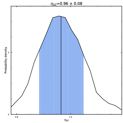
Appendix B Comparison between MILCA and forward-modeling pressure profiles

To test the robustness of our pressure profile measurements, we compared the MILCA results with the pressure measured using an alternative technique (see Bourdin et al. 2017). Following this technique, Planck-HFI frequency maps are first wavelet cleaned for CMB and thermal dust anisotropies, a parametric pressure template (Nagai et al. 2007) is subsequently projected onto the sky plane, convolved with the frequency dependent HFI beams and fitted to the CMB and dust cleaned maps. Being fully parametric, this technique allow us to take advantage of the frequency dependent angular resolution of each HFI channel during the template fitting. This angular resolution is about 9.7 and 7.3 arcmin at 100 and 143 GHz, respectively, but reaches about 5 arcmin in the energy range [217, 857] GHz (Planck Collaboration et al. 2016b).

In Fig. 10 we compare the resulting best fitting pressure profile from the above procedure with the MILCA maps (see Sect. 2.5). The residuals are shown in the left panel and show the nice agreement, within the statistical uncertainty, of the two different methods applied. In the right panel all the residuals are grouped together to create a distribution, which is compared with a Gaussian centered at 0 and width 1, showing that the residuals follow this distribution very closely, indicating that statistically the two pressure profiles are in very good agreement.

Figure 10: Left: Residuals of the comparison of the two different methods we used to estimate the SZ pressure profile. A remarkable good agreement within the statistical uncertainties is reached at all radii, especially excluding the first 3 MILCA points which are the most affected by the Planck PSF. Right: Distribution of the residuals compared with the statistical prediction of a set of residuals: a gaussian centered in zero and width one (red line).

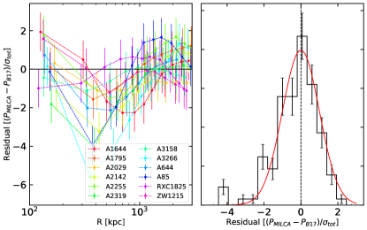
Appendix C Mass-induced scatter in thermodynamic profiles

Since the scaling of our thermodynamic quantities depends on the cluster mass both through the scale radius $R_{500}$ and the self-similar quantities $Q_{500}$ (see Sect. 3), the measured scatter profiles presented in Fig. 7 depend on the accuracy of the adopted masses. Both statistical and systematic fluctuations of the measured mass around the true mass will induce fluctuations of the scaling quantities, thus introducing an irreducible source of scatter originating from the limited accuracy of our mass calibration.

To take this effect into account, we estimated numerically the scatter in each quantity that is induced by uncertainties in our mass scaling. We started from scatter-free universal profiles following the measurements provided in Table 3, and perturbed the mass scaling according to the known statistical uncertainties and biases in our mass scaling. Namely, for each X-COP cluster we randomly drew new values of the observed mass $M_{\rm obs}$ as

$$M_{\rm obs}=\mbox{Gauss}((1-b)M_{\rm true},\Delta M)$$ (15)

with $M_{\rm true}$ the assumed true mass, $b$ the hydrostatic mass bias, and $\Delta M$ the statistical uncertainty in our hydrostatic masses (see Ettori et al. 2018 for details). For the hydrostatic mass bias, we used the distribution of non-thermal pressure values determined in Eckert et al. (2018) from the measured gas fraction. We then scaled the scatter-free profiles for each quantity $Q$ by the perturbed values of $R_{500}$ and $Q_{500}$.

We applied this procedure to each X-COP cluster and computed the resulting scatter as a function of radius. We repeated this procedure 1,000 times to get an idea of the uncertainty introduced by sample variance. In Fig. 11 we show the resulting mass-induced scatter for the scaled pressure, density, temperature, and entropy. We can see that the effect of the mass scaling is largest on the pressure and ranges between 6% and 12% as a function of radius. Conversely, the effect on the entropy is minimal (2%–3%). The scatter in temperature and density induced by uncertainties in the mass scaling lies somewhere in between. Pressure is more affected than the other thermodynamic quantities simply because its slope is the most steep among the quantities.

Figure 11: Scatter in the various thermodynamic profiles induced by uncertainties in the mass calibration. The shaded areas show the range of intrinsic scatter obtained from 1,000 simulations.

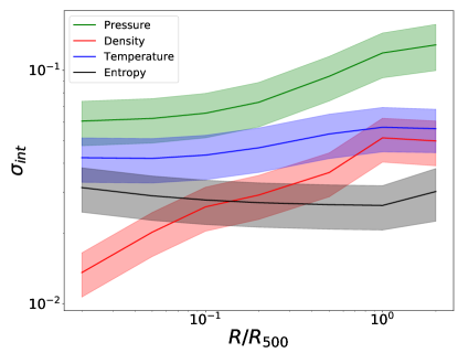
Appendix D Piecewise power law fits for CC and NCC clusters separately

In Fig. 12 and Table 4 we show the results of piecewise power law fits to the X-COP clusters divided into the CC and NCC populations. In Fig. 13 we also show the best fit scatter of the populations as a function of radius, split into CC and NCC clusters and compared with the full population. In this case, we caution that the number of systems in each category is small (four CC and eight NCC systems) and the measurements of the scatter may be unreliable.

Figure 12: Same as Fig. 8, but using the piecewise fit instead of global functional form. The cluster population of X-COP is divided into cool-core (CC, in blue) and non-cool-core clusters (NCC, in red), compared with the entire population (ALL, in green).

Table 4: Same as Table 2, but discriminating between cool-core and non-cool-core clusters.

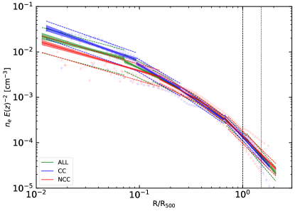
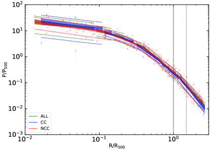
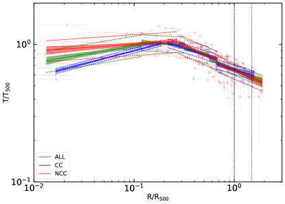
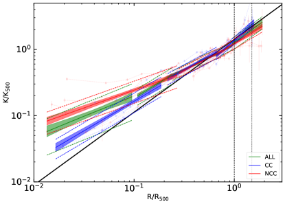
Density

cool-cores (CC)					Non-cool-cores (NCC)
$x_{in}$	$x_{out}$	A ($10^{-4}$ cm-3)	B (slope)	$\sigma_{int}$	$x_{in}$	$x_{out}$	A	B (slope)	$\sigma_{int}$
0.01	0.09	$10.16\pm 3.26$	$-0.80\pm 0.10$	$0.42\pm 0.04$	0.01	0.16	$8.33\pm 1.27$	$-0.66\pm 0.06$	$0.40\pm 0.03$
0.09	0.25	$2.46\pm 0.64$	$-1.32\pm 0.14$	$0.31\pm 0.03$	0.16	0.34	$2.66\pm 0.29$	$-1.21\pm 0.08$	$0.19\pm 0.01$
0.25	0.65	$1.68\pm 0.13$	$-1.56\pm 0.08$	$0.18\pm 0.02$	0.35	0.72	$1.75\pm 0.08$	$-1.64\pm 0.07$	$0.16\pm 0.01$
0.67	1.81	$1.31\pm 0.03$	$-2.47\pm 0.09$	$0.15\pm 0.02$	0.72	2.09	$1.39\pm 0.04$	$-2.23\pm 0.10$	$0.30\pm 0.02$

Pressure

cool-cores (CC)					Non-cool-cores (NCC)
$x_{in}$	$x_{out}$	A	B (slope)	$\sigma_{int}$	$x_{in}$	$x_{out}$	A	B (slope)	$\sigma_{int}$
0.02	0.11	$6.23\pm 2.63$	$-0.31\pm 0.15$	$0.76\pm 0.13$	0.01	0.15	$3.85\pm 1.51$	$-0.40\pm 0.13$	$0.48\pm 0.07$
0.12	0.29	$1.12\pm 0.48$	$-0.97\pm 0.25$	$0.26\pm 0.06$	0.16	0.37	$0.77\pm 0.23$	$-1.18\pm 0.21$	$0.33\pm 0.04$
0.32	0.66	$0.30\pm 0.05$	$-1.98\pm 0.23$	$0.20\pm 0.05$	0.39	0.71	$0.26\pm 0.06$	$-2.36\pm 0.37$	$0.36\pm 0.05$
0.69	1.17	$0.22\pm 0.02$	$-2.52\pm 0.35$	$0.19\pm 0.05$	0.71	1.08	$0.26\pm 0.03$	$-2.07\pm 0.58$	$0.39\pm 0.06$
1.23	2.65	$0.30\pm 0.07$	$-3.54\pm 0.39$	$0.31\pm 0.10$	1.12	2.50	$0.27\pm 0.05$	$-3.03\pm 0.36$	$0.43\pm 0.08$

Temperature

cool-cores (CC)					Non-cool-cores (NCC)
$x_{in}$	$x_{out}$	A	B (slope)	$\sigma_{int}$	$x_{in}$	$x_{out}$	A	B (slope)	$\sigma_{int}$
0.02	0.19	$1.40\pm 0.05$	$0.19\pm 0.01$	$0.04\pm 0.01$	0.01	0.27	$1.13\pm 0.09$	$0.05\pm 0.03$	$0.17\pm 0.02$
0.22	0.66	$0.72\pm 0.04$	$-0.23\pm 0.05$	$0.07\pm 0.02$	0.28	0.68	$0.68\pm 0.05$	$-0.31\pm 0.09$	$0.15\pm 0.02$
0.66	1.57	$0.66\pm 0.02$	$-0.22\pm 0.10$	$0.08\pm 0.03$	0.69	1.90	$0.64\pm 0.02$	$-0.31\pm 0.10$	$0.13\pm 0.02$

Entropy

cool-cores (CC)					Non-cool-cores (NCC)
$x_{in}$	$x_{out}$	A	B (slope)	$\sigma_{int}$	$x_{in}$	$x_{out}$	A	B (slope)	$\sigma_{int}$
0.02	0.19	$1.30\pm 0.29$	$0.90\pm 0.08$	$0.33\pm 0.05$	0.01	0.27	$0.83\pm 0.14$	$0.54\pm 0.06$	$0.37\pm 0.04$
0.22	0.66	$1.26\pm 0.16$	$0.81\pm 0.12$	$0.19\pm 0.03$	0.28	0.68	$1.19\pm 0.09$	$0.78\pm 0.09$	$0.15\pm 0.02$
0.66	1.57	$1.37\pm 0.06$	$1.32\pm 0.17$	$0.12\pm 0.04$	0.69	1.90	$1.22\pm 0.04$	$0.92\pm 0.13$	$0.17\pm 0.03$

Table 5: Stacked thermodynamic profiles. $N_{X}$ and $N_{SZ}$ indicates the number or objects reaching the indicated radius in X.ray and SZ data respectively. We indicate the median of the 12 cluster profiles, and with the subscripts _low and _high we indicate the values that contain 68% of the objects.

Density
$\frac{R}{R_{500}}$	$n_{e}E(z)^{-2}$	$(n_{e}E(z)^{-2})_{low}$	$(n_{e}E(z)^{-2})_{high}$	$N_{X}$
-	cm-3	cm-3	cm-3	-
1.058e-02	8.814e-03	6.543e-03	1.503e-02	12
1.179e-02	8.751e-03	6.224e-03	1.416e-02	12
1.313e-02	8.684e-03	6.018e-03	1.457e-02	12
1.463e-02	8.712e-03	5.929e-03	1.421e-02	12
1.630e-02	8.409e-03	5.839e-03	1.324e-02	12
1.816e-02	8.110e-03	5.666e-03	1.269e-02	12
2.024e-02	8.007e-03	5.560e-03	1.314e-02	12
2.255e-02	7.720e-03	5.432e-03	1.100e-02	12
2.513e-02	7.627e-03	5.440e-03	1.167e-02	12
2.799e-02	7.593e-03	5.445e-03	1.165e-02	12
3.119e-02	7.513e-03	5.503e-03	1.133e-02	12
3.475e-02	7.334e-03	5.534e-03	1.089e-02	12
3.872e-02	7.086e-03	5.271e-03	1.058e-02	12
4.314e-02	6.889e-03	5.086e-03	1.000e-02	12
4.807e-02	6.675e-03	4.839e-03	9.519e-03	12
5.356e-02	6.408e-03	4.531e-03	8.860e-03	12
5.967e-02	6.161e-03	4.246e-03	8.219e-03	12
6.649e-02	5.628e-03	3.817e-03	7.509e-03	12
7.408e-02	5.255e-03	3.550e-03	6.841e-03	12
8.254e-02	4.875e-03	3.359e-03	6.049e-03	12
9.197e-02	4.473e-03	3.196e-03	5.461e-03	12
1.025e-01	4.141e-03	2.992e-03	4.983e-03	12
1.142e-01	3.813e-03	2.728e-03	4.495e-03	12
1.272e-01	3.429e-03	2.527e-03	4.023e-03	12
1.417e-01	3.011e-03	2.327e-03	3.565e-03	12
1.579e-01	2.678e-03	2.123e-03	3.089e-03	12
1.759e-01	2.385e-03	1.854e-03	2.676e-03	12
1.960e-01	2.142e-03	1.650e-03	2.296e-03	12
2.184e-01	1.892e-03	1.478e-03	1.992e-03	12
2.434e-01	1.675e-03	1.328e-03	1.723e-03	12
2.712e-01	1.444e-03	1.159e-03	1.475e-03	12
3.021e-01	1.193e-03	1.038e-03	1.238e-03	12
3.366e-01	1.013e-03	9.677e-04	1.039e-03	12
3.751e-01	8.583e-04	8.375e-04	8.741e-04	12
4.179e-01	7.145e-04	6.885e-04	7.349e-04	12
4.656e-01	5.997e-04	5.689e-04	6.211e-04	12
5.188e-01	4.926e-04	4.631e-04	5.208e-04	12
5.780e-01	4.043e-04	3.744e-04	4.390e-04	12
6.440e-01	3.391e-04	3.190e-04	3.530e-04	12
7.176e-01	2.742e-04	2.657e-04	2.832e-04	12
7.995e-01	2.199e-04	2.106e-04	2.277e-04	12
8.908e-01	1.783e-04	1.691e-04	1.843e-04	12
9.925e-01	1.423e-04	1.312e-04	1.493e-04	12
1.106e+00	1.142e-04	1.051e-04	1.213e-04	11
1.232e+00	8.635e-05	7.469e-05	9.571e-05	11
1.373e+00	6.274e-05	5.512e-05	6.934e-05	11
1.530e+00	4.767e-05	4.269e-05	5.336e-05	10
1.704e+00	3.720e-05	3.132e-05	4.402e-05	5
1.899e+00	2.769e-05	2.355e-05	3.228e-05	2
Continued on next page

Table 5: continued.

Pressure
$\frac{R}{R_{500}}$	$\left(\frac{P}{P_{500}}\right)_{X}$	$\left(\frac{P}{P_{500}}\right)_{X,low}$	$\left(\frac{P}{P_{500}}\right)_{X,high}$	$N_{X}$	$\left(\frac{P}{P_{500}}\right)_{SZ}$	$\left(\frac{P}{P_{500}}\right)_{SZ,low}$	$\left(\frac{P}{P_{500}}\right)_{SZ,high}$	$N_{SZ}$
2.283e-02	2.396e+01	1.380e+01	2.829e+01	10	-	-	-	-
2.909e-02	2.110e+01	1.243e+01	2.603e+01	10	-	-	-	-
3.706e-02	2.198e+01	1.420e+01	2.376e+01	11	-	-	-	-
4.723e-02	1.995e+01	1.447e+01	2.123e+01	11	-	-	-	-
6.018e-02	1.569e+01	1.025e+01	1.847e+01	12	-	-	-	-
7.669e-02	1.318e+01	8.647e+00	1.557e+01	12	-	-	-	-
9.772e-02	1.086e+01	7.665e+00	1.283e+01	12	-	-	-	-
1.245e-01	8.800e+00	7.024e+00	1.022e+01	12	-	-	-	-
1.587e-01	6.847e+00	5.763e+00	7.680e+00	12	-	-	-	-
2.022e-01	5.144e+00	4.492e+00	5.694e+00	12	-	-	-	-
2.577e-01	3.896e+00	3.390e+00	4.181e+00	12	-	-	-	-
3.283e-01	2.702e+00	2.537e+00	2.837e+00	12	-	-	-	-
4.184e-01	1.834e+00	1.748e+00	1.921e+00	12	-	-	-	-
5.331e-01	1.093e+00	1.059e+00	1.152e+00	12	9.885e-01	9.060e-01	1.077e+00	11
6.794e-01	6.140e-01	5.636e-01	6.594e-01	12	6.075e-01	5.461e-01	6.765e-01	12
8.657e-01	3.260e-01	2.643e-01	3.803e-01	8	3.571e-01	3.031e-01	4.056e-01	12
1.103e+00	-	-	-	-	1.939e-01	1.562e-01	2.242e-01	12
1.406e+00	-	-	-	-	9.760e-02	7.288e-02	1.132e-01	12
1.791e+00	-	-	-	-	4.649e-02	3.710e-02	5.343e-02	11

Temperature
$\frac{R}{R_{500}}$	$\left(\frac{T}{T_{500}}\right)_{X}$	$\left(\frac{T}{T_{500}}\right)_{X,low}$	$\left(\frac{T}{T_{500}}\right)_{X,high}$	$N_{X}$	$\left(\frac{T}{T_{500}}\right)_{SZ}$	$\left(\frac{T}{T_{500}}\right)_{SZ,low}$	$\left(\frac{T}{T_{500}}\right)_{SZ,high}$	$N_{SZ}$
2.283e-02	7.606e-01	7.049e-01	8.741e-01	10	-	-	-	-
2.909e-02	7.776e-01	7.338e-01	8.823e-01	10	-	-	-	-
3.706e-02	8.259e-01	7.814e-01	9.534e-01	11	-	-	-	-
4.723e-02	8.485e-01	8.086e-01	9.598e-01	11	-	-	-	-
6.018e-02	8.759e-01	8.434e-01	9.510e-01	12	-	-	-	-
7.669e-02	9.102e-01	8.705e-01	9.650e-01	12	-	-	-	-
9.772e-02	9.460e-01	9.028e-01	9.913e-01	12	-	-	-	-
1.245e-01	9.669e-01	9.314e-01	1.011e+00	12	-	-	-	-
1.587e-01	9.717e-01	9.425e-01	1.021e+00	12	-	-	-	-
2.022e-01	9.816e-01	9.354e-01	1.024e+00	12	-	-	-	-
2.577e-01	9.751e-01	9.518e-01	1.005e+00	12	-	-	-	-
3.283e-01	9.540e-01	9.347e-01	9.794e-01	12	-	-	-	-
4.184e-01	9.317e-01	8.946e-01	9.662e-01	12	-	-	-	-
5.331e-01	8.714e-01	8.409e-01	8.970e-01	12	7.616e-01	7.053e-01	8.134e-01	11
6.794e-01	7.529e-01	7.093e-01	7.937e-01	12	7.253e-01	6.779e-01	7.748e-01	12
8.657e-01	6.540e-01	6.061e-01	6.917e-01	8	6.872e-01	6.461e-01	7.280e-01	12
1.103e+00	-	-	-	-	6.381e-01	6.001e-01	6.673e-01	12
1.406e+00	-	-	-	-	5.664e-01	5.317e-01	6.012e-01	11
1.791e+00	-	-	-	-	4.852e-01	4.380e-01	5.406e-01	6

Entropy
$\frac{R}{R_{500}}$	$\left(\frac{K}{K_{500}}\right)_{X}$	$\left(\frac{K}{K_{500}}\right)_{X,low}$	$\left(\frac{K}{K_{500}}\right)_{X,high}$	$N_{X}$	$\left(\frac{K}{K_{500}}\right)_{SZ}$	$\left(\frac{K}{K_{500}}\right)_{SZ,low}$	$\left(\frac{K}{K_{500}}\right)_{SZ,high}$	$N_{SZ}$
2.283e-02	9.245e-02	5.696e-02	1.159e-01	10	-	-	-	-
2.909e-02	1.058e-01	5.736e-02	1.192e-01	10	-	-	-	-
3.706e-02	1.116e-01	7.998e-02	1.377e-01	11	-	-	-	-
4.723e-02	1.303e-01	8.800e-02	1.516e-01	11	-	-	-	-
6.018e-02	1.455e-01	1.059e-01	1.643e-01	12	-	-	-	-
7.669e-02	1.701e-01	1.403e-01	1.863e-01	12	-	-	-	-
9.772e-02	2.024e-01	1.745e-01	2.263e-01	12	-	-	-	-
1.245e-01	2.367e-01	2.107e-01	2.637e-01	12	-	-	-	-
1.587e-01	2.879e-01	2.584e-01	3.121e-01	12	-	-	-	-
2.022e-01	3.412e-01	3.060e-01	3.960e-01	12	-	-	-	-
2.577e-01	4.147e-01	3.895e-01	4.615e-01	12	-	-	-	-
3.283e-01	4.881e-01	4.737e-01	5.074e-01	12	-	-	-	-
4.184e-01	6.452e-01	5.985e-01	6.999e-01	12	-	-	-	-
5.331e-01	7.886e-01	7.595e-01	8.156e-01	12	6.631e-01	6.304e-01	6.973e-01	11
6.794e-01	8.852e-01	8.467e-01	9.227e-01	12	8.607e-01	8.225e-01	8.982e-01	12
8.657e-01	1.027e+00	9.461e-01	1.104e+00	8	1.107e+00	1.046e+00	1.168e+00	12
1.103e+00	-	-	-	-	1.460e+00	1.360e+00	1.569e+00	12
1.406e+00	-	-	-	-	2.060e+00	1.779e+00	2.389e+00	11
1.791e+00	-	-	-	-	2.774e+00	1.658e+00	4.491e+00	6

Figure 13: Scatter of our thermodynamic quantities dividing our cluster sample in CC and NCC

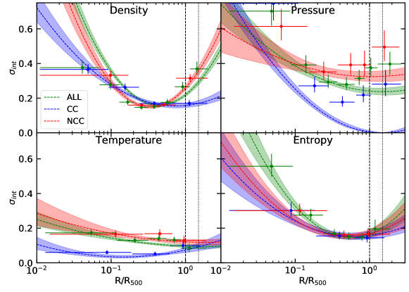
Appendix E Marginalized posterior likelihood

Figure 14: Parameter distribution for the best fit on the density of all clusters using the Vikhlinin et al. (2006) functional form, Eq. (7). The priors on the parameters are shown in Table 3.

Figure 15: Parameter distribution for the best fit on the pressure of all clusters using the Nagai et al. (2007) gNFW functional form, Eq. (9), fixing the intermediate slope $\alpha$. The priors on the parameters are shown in Table 3.

Figure 16: Parameter distribution for the best fit on the temperature of all clusters using the Vikhlinin et al. (2006) functional form, Eq. (11). The priors on the parameters are shown in Table 3.

Figure 17: Parameter distribution for the best fit on the entropy of all clusters using a power law plus constant functional form, Eq. (13). The priors on the parameters are shown in Table 3.

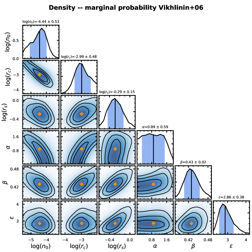
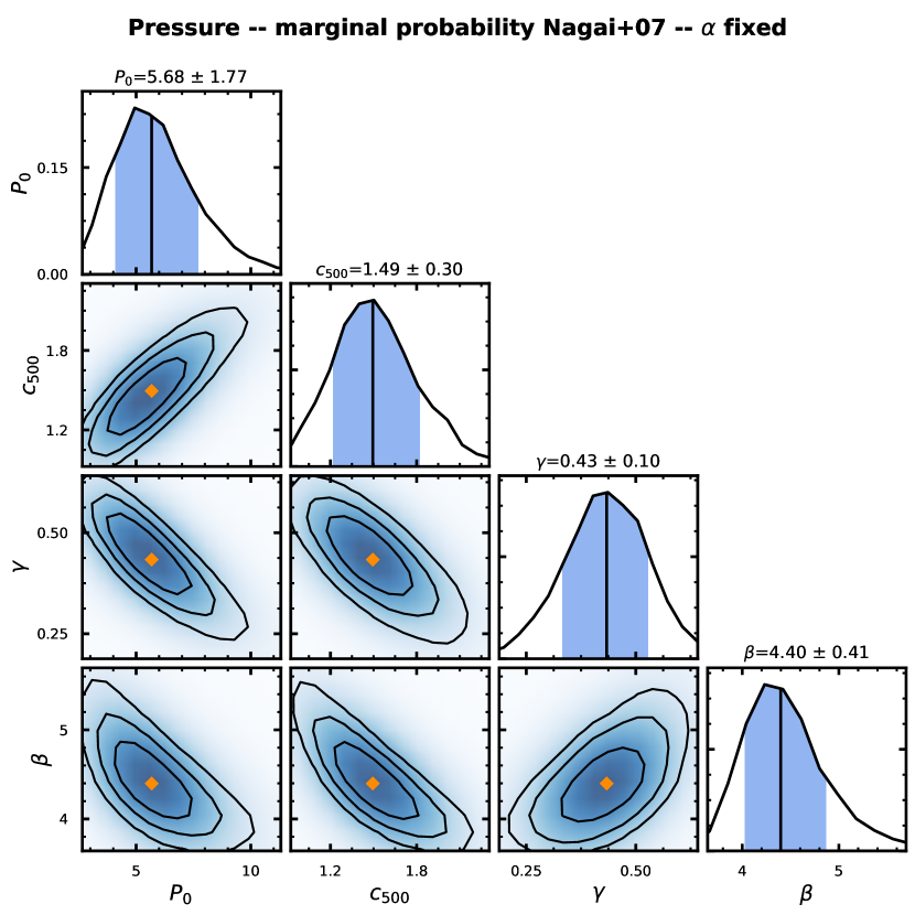
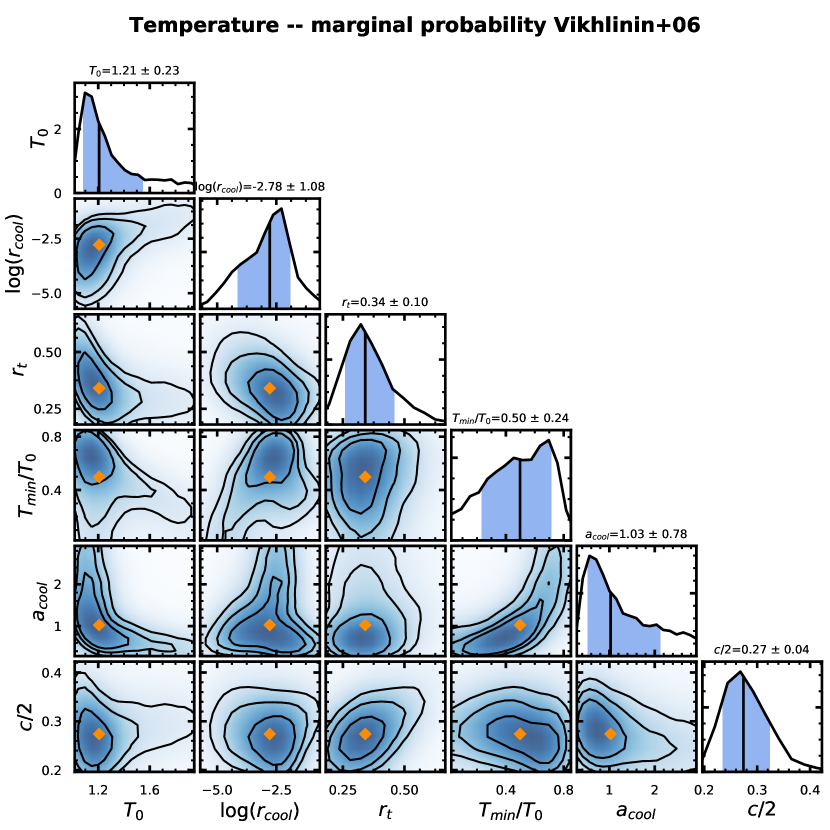
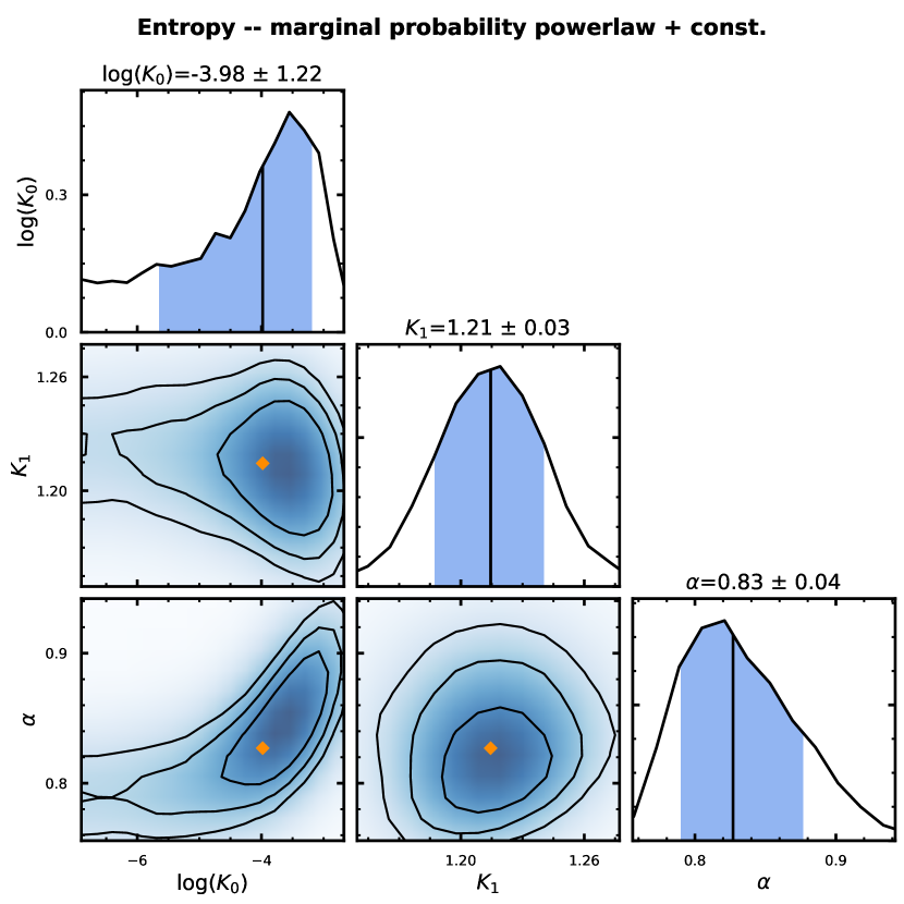
Appendix F Log of scientific observations

Table 6: Log of X-COP observations.

Target	Obs.Id.	Obs.Date	$N_{H}$	$t_{M1}$	$t_{M2}$	$t_{pn}$
		[yr/mm/dd]	[$10^{20}\rm cm^{-2}$]	[ks]	[ks]	[ks]
A1644 Center	0010420201	2001-01-08	4.2	13.5	13.6	11.9
A1644 E	0744413001	2015-01-01	4.3	15.5	17.5	10.3
A1644 N	0744412701	2014-12-29	3.9	27.5	28.4	14.8
A1644 S	0744412901	2014-12-31	4.4	10.2	11.3	4.7
A1644 W	0744412801	2015-06-30	3.8	29.2	28.7	21.7
A1795 Center	0097820101	2000-06-26	1.2	36.1	36.5	26.0
A1795 E	0744412101	2015-06-16	1.2	19.3	25.1	10.4
A1795 N	0744412001	2015-01-05	1.2	15.3	16.3	11.2
A1795 NW	0205190201	2004-01-25	1.2	22.5	22.9	21.1
A1795 S	0109070201	2003-01-13	1.2	52.6	53.5	52.1
A1795 W	0205190101	2004-01-25	1.1	29.2	28.9	27.0
A2029 Center 1	0551780201	2008-07-17	3.2	33.1	34.0	15.1
A2029 Center 2	0551780301	2008-07-19	3.2	39.0	40.9	27.4
A2029 E	0744411201	2015-01-31	3.2	26.0	26.7	20.6
A2029 N	0744410901	2015-02-08	3.0	17.5	22.3	6.6
A2029 S	0744411101	2015-02-22	3.4	11.0	16.6	4.9
A2029 W	0744411001	2015-07-27	3.2	42.6	43.3	39.2
A2142 Center	0674560201	2011-07-13	3.8	52.3	53.8	48.8
A2142 NE	0694440201	2012-07-14	3.8	33.2	33.1	29.8
A2142 NW	0694440101	2012-07-14	3.7	19.6	18.5	12.5
A2142 SE	0694440501	2012-07-16	4.0	33.2	32.5	29.8
A2142 SW	0694440601	2012-07-18	3.9	30.3	31.5	24.1
A2255 E	0744410801	2014-03-30	2.5	12.1	17.8	9.4
A2255 N	0744410501	2014-03-14	2.5	14.0	19.9	7.5
A2255 S	0744410701	2014-03-28	2.5	23.4	23.8	12.4
A2255 W	0744410601	2014-04-27	2.4	28.6	30.2	22.1
A2255 Center	0112260801	2002-12-07	2.5	7.7	8.2	2.3
A2319 E	0744410401	2014-04-08	9.1	14.5	15.9	10.9
A2319 N	0744410101	2014-03-15	8.8	23.9	24.2	21.8
A2319 S	0744410301	2014-04-04	8.2	13.8	14.3	8.2
A2319 W	0744410201	2014-04-09	7.7	23.8	25.4	11.1
A2319 Center 1	0302150101	2005-10-10	8.1	15.7	15.6	10.6
A2319 Center 2	0302150201	2005-11-14	8.1	16.0	15.5	12.4
A3158 Center	0300210201	2005-11-22	1.4	19.8	19.7	11.2
A3158 E	0744411601	2015-08-29	1.4	31.2	31.7	26.2
A3158 N	0744411301	2014-11-12	1.3	28.1	28.6	21.5
A3158 S	0744411501	2015-05-31	1.3	28.0	28.6	19.3
A3158 W	0744411401	2015-03-01	1.3	20.8	20.2	16.4
A3266 f1	0105260701	2000-10-01	1.5	19.1	19.5	15.5
A3266 f2	0105260801	2000-10-11	1.5	19.6	19.6	15.5
A3266 f3	0105260901	2000-10-09	1.6	23.4	23.1	17.9
A3266 f4	0105262201	2000-09-27	1.5	3.0	2.9	3.2
A3266 f5	0105262101	2000-09-25	1.8	5.8	6.1	4.1
A3266 f5b	0105261101	2000-09-25	1.8	11.3	12.3	7.1
A3266 f6	0105262001	2000-09-23	1.7	6.2	5.6	2.5
A3266 f6c	0105262501	2003-03-15	1.7	6.3	6.8	3.1
A644 Center	0744412201	2014-04-07	7.5	19.7	25.4	11.8
A644 E	0744412601	2014-05-18	6.7	20.5	24.3	8.6
A644 N	0744412301	2014-10-22	7.4	35.1	35.8	30.3
A644 S	0744412501	2014-10-24	7.0	32.3	32.2	26.2
A644 W	0744412401	2015-04-08	7.5	30.6	30.4	18.9
A85 Center	0723802201	2013-06-18	2.8	95.8	97.9	85.2
A85 E	0744411901	2014-12-11	2.8	28.2	29.0	19.5
A85 N	0744411701	2015-01-12	2.9	22.0	23.4	14.8
A85 S	0065140201	2002-01-07	2.7	12.2	12.1	9.4
A85 W	0744411801	2015-06-06	2.8	28.4	28.2	21.1
A85 NW	0744930301	2014-06-23	2.8	29.2	30.4	21.0
RXCJ1825 Center	0744413501	2014-04-11	9.4	48.1	48.2	39.1
RXCJ1825 E	0744413901	2014-04-13	10.0	31.7	32.4	16.2
RXCJ1825 N	0744413601	2014-04-12	8.9	20.0	20.2	14.3
RXCJ1825 S	0744413801	2014-04-14	9.5	25.5	29.5	12.4
RXCJ1825 W	0744413701	2014-10-02	9.2	41.4	40.8	36.8
ZwCl1215 Center	0300211401	2006-06-24	1.7	23.3	24.0	16.3
ZwCl1215 E	0744413401	2015-12-17	1.7	26.0	26.0	21.1
ZwCl1215 N	0744413101	2014-12-06	1.7	18.2	18.5	10.1
ZwCl1215 S	0744413301	2015-06-04	1.8	28.9	28.7	24.4
ZwCl1215 W	0744413201	2015-06-11	1.8	21.4	24.2	12.9

Table 6: continued.

Columns: 1. Target name; 2. Observation identifier; 3. Observation date; 4. Equivalent hydrogen column density as estimated from 21 cm maps (Kalberla et al. 2005); 4. Exposure time for MOS1 detector after flare removal; 5. Exposure time for MOS2 detector after flare removal; 6. Exposure time for pn detector after flare removal.