1 Introduction
Stochastic partial differential equations (SPDEs) are widely used to mathematically model random phenomena
appearing in the fields of physics, chemistry, biology, finance and many other branches of science.
Over the past decades, there have been plenty of research articles analyzing numerical discretizations of
parabolic SPDEs, see, e.g., monographs lord2014introduction ; kruse2014strong
and references therein. In contrast to an overwhelming majority of literature
focusing on numerical analysis of SPDEs with globally Lipschitz nonlinearity,
only a limited number of papers investigated numerical SPDEs in the non-globally Lipschitz regime
becker2017strong ; brehier2018strong ; brehier2018analysis ; brehier2018weak ; feng2017finite ; gyongy2016convergence ; jentzen2015strong ; kovacs2015discretisation ; becker2016strong ; hutzenthaler2016strong ; jentzen2016exponential ; liu2018strong ; kovacs2015backward and it is still far from being well-understood.
As a typical example of parabolic SPDEs with non-globally Lipschitz nonlinearity, stochastic Allen-Cahn equations,
perturbed by additive or multiplicative noises, have received increasing attention in the last few years.
Recently, several research works were reported on numerical approximations of such equations
feng2017finite ; katsoulakis2011noise ; kovacs2015backward ; liu2017wong ; liu2018strong ; brehier2018strong ; Majee2017optimal ; brehier2018weak ; wang2018efficient ; brehier2018analysis ; kovacs2015discretisation .
The present work makes further contributions in this direction,
by successfully recovering optimal strong convergence rates for finite element semi-discretization and spatio-temporal
full discretization of stochastic Allen-Cahn equations with additive noise, including both the space-time white noise in
space dimension and the trace-class noise in multiple space dimensions.
Let be a bounded open spatial domain with smooth boundary
and let be the real separable Hilbert space endowed with usual inner product
and norm.
Throughout this article we are interested in the following semi-linear parabolic SPDE in ,
|
|
|
(1.1) |
where is a linear, densely defined,
positive self-adjoint unbounded operator with compact inverse (e.g., with homogeneous Dirichlet boundary condition)
in , generating an analytic semigroup in .
Moreover, is an -valued (possibly cylindrical) -Wiener process on a filtered probability space
with respect to the normal filtration .
The nonlinear mapping is assumed to be a Nemytskij operator, given by
Such problem is often referred to as stochastic Allen-Cahn equation.
Under further assumptions specified later, particularly including
|
|
|
(1.2) |
it is proved in Theorems 2.1, 2.2 that the problem (1.1) possesses a unique mild solution,
|
|
|
(1.3) |
which enjoys the Sobolev and Hölder regularity properties
|
|
|
(1.4) |
and
for and ,
|
|
|
(1.5) |
Here stands for the Hilbert-Schmidt norm,
and the parameter coming from (1.2)
quantifies
the spatial regularity of the covariance operator of the driving noise process
(Assumption 2.3). The setting covers both the space-time white noise in space dimension
and the trace-class noise in multiple space dimensions (see Remark 1 for details).
The obtained space-time regularity coincides with that in kruse2012optimal for SPDEs with globally Lipschitz nonlinearity
and is thus optimal in the spirit of kruse2012optimal .
Let , be an open convex polynomial domain and
with . Let be a finite element space
of piecewise continuous linear functions
and the finite element spatial approximation of the mild solution , which can be represented by
|
|
|
(1.6) |
Here is the strongly continuous semigroup generated by the discrete Laplace operator .
The resulting spatial approximation error is measured as follows (Theorem 3.1)
|
|
|
(1.7) |
where is determined by the assumption (1.2).
The obtained convergence rate in space is called optimal since it exactly coincides with the order of
optimal spatial regularity of the solution (thomee2006galerkin, , Chapter 1).
Discretizing the semi-discrete problem by a backward Euler time-stepping scheme, we also investigate
a fully discrete scheme for (1.3), given by
|
|
|
(1.8) |
where is the fully discrete approximations of and .
Equivalently, the one-step recursion (1.8) can be reformulated as
|
|
|
(1.9) |
As stated in Theorem 4.1,
the corresponding strong approximation error reads,
|
|
|
(1.10) |
This indicates how the strong convergence rate of the full discretization relies on the regularity of the driven noise process.
Particularly when the condition (1.2) is fulfilled with , a classical convergence rate of order
for the backward Euler-finite element full discretization is reachable, even in multiple spatial dimensions
(see Remark 1). These findings are identical to those in wang2017strong ,
where the strong convergence rate of the linear implicit Euler finite element scheme was analyzed for SPDEs with globally Lipschitz nonlinearity.
Once the nonlinearity grows super-linearly, one can in general not expect the usual nonlinearity-explicit time-stepping schemes
that work well in the globally Lipschitz setting converge in the strong sense (see comments following Theorem 2 in jentzen2009pathwise
and the relavant divergence result hutzenthaler2011strong ).
To address this issue, we therefore take the backward Euler, a nonlinearity-implicit scheme, for the temporal discretization.
Although some error estimates are taken from kruse2012optimal ; kruse2014optimal ; wang2017strong ,
the presence of the non-globally Lipschitz (cubic) nonlinearity in the underlying model brings about essential difficulties in
the error analysis (see the proof of Theorems 3.1, 4.1)
and the error analysis becomes much more involved than that in the globally Lipschitz SPDE setting.
In the following, we take error estimates of the spatial semi-discretization to illuminate our approach of the error analysis.
By introducing an auxiliary approximation process , defined by
|
|
|
(1.11) |
we separate the spatial error into two parts,
|
|
|
(1.12) |
Subtracting (1.11) from (1.3), one can treat the first error term
directly and get ,
with the aid of existing estimates for the error operators
and regularity properties of the mild solution
(see estimates of in the proof of Theorem 3.1 for details).
To bound the remaining error term , we subtract
(1.6) from (1.11) to eliminate the stochastic convolution and thus
is time differentiable and satisfies
|
|
|
(1.13) |
Deterministic calculus together with the monotonicity of the nonlinearity, regularity properties of ,
the previous estimate of and Gronwall’s inequality facilitates the derivation of
(see (3.32)-(3.34)).
In the same manner as the semi-discrete case, we introduce an auxiliary process
|
|
|
(1.14) |
and decompose the full discretization error as
|
|
|
(1.15) |
Then following the basic line as above, but with much more efforts made to exploit discrete versions of arguments
as used in the semi-discrete scenario, enables us to attain the desired error bounds for the full discretization
(cf. section 4).
As usual, the strong convergence rate analysis of numerical SPDEs with super-linearly growing nonlinearities are
carried out based on appropriate uniform a priori moment -bounds of approximations becker2017strong ; liu2018strong ; feng2017finite ; Majee2017optimal .
Originally we develop a new approach of error analysis here, which does not rely on
high-order spatial regularity properties (e.g., a priori moment -bounds) of approximation processes , .
As already illustrated above, the new approach proposed for the error analysis is easy to understand
and can be extended to the error analysis for the stochastic Cahn-Hilliard equation kovacs2011finite ; furihata2018strong ; qi2018strong .
Before closing the introduction part, we recall a few existing closely relevant works.
The backward Euler time semi-discretization was also examined in kovacs2015backward ; kovacs2015discretisation
for the problem (1.1), with no spatial discretization. Under assumption (1.2) taking ,
i.e., ,
only a strong convergence rate of order was attained in kovacs2015discretisation .
In brehier2018analysis ; brehier2018strong ; brehier2018weak , pure time semi-discretizations of splitting type were studied
for (1.1). Particularly, the authors of brehier2018strong used exponential integrability properties of exact and
numerical solutions to identify a strong convergence rate of order , but only valid in one space dimension,
when the additive noise is moderately smooth, i.e., in (1.2).
Besides, various discretizations were investigated in becker2017strong ; becker2016strong ; liu2018strong ; wang2018efficient
for the space-time white noise case
and in feng2017finite ; Majee2017optimal for the multiplicative one-dimensional noise case (gradient type noise in feng2017finite ),
only involved with a standard -valued Brownian motion.
The outline of this paper is as follows. In the next section, some preliminaries are collected and the
well-posedness and regularity properties of the considered problem are elaborated.
Section 3 is devoted to error estimates of the finite element spatial semi-discretization
and section 4 provides error estimates of the backward Euler-finite element full discretization.
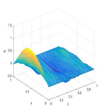
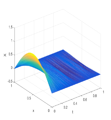
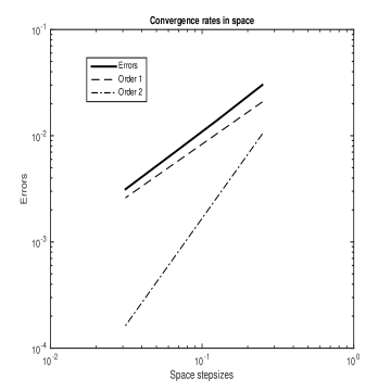
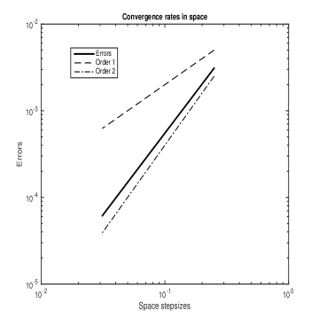
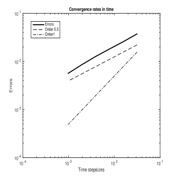
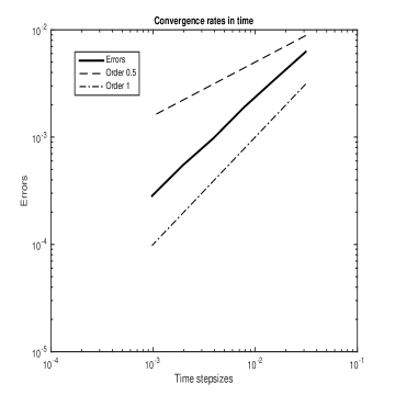
At the end of the article, some numerical examples are presented, illustrating the above theoretical findings.
3 Error estimates of the spatial semi-discretization
This section is devoted to error estimates of the finite element approximation of the stochastic problem (1.1).
For the sake of simplicity, from here to section 4 we always assume that , is an open convex polynomial domain and with .
In order to introduce the semi-discrete finite element approximation,
we present some notation and operators on the finite element space. Let , be the space of
continuous functions that are piecewise linear over the triangulation of .
Then we introduce a discrete Laplace operator defined by
|
|
|
(3.1) |
and a generalized projection operator given by
|
|
|
(3.2) |
It is well-known that, the operators and obey
|
|
|
(3.3) |
The semi-discrete finite element method for the problem (1.1) is to find such that
|
|
|
(3.4) |
Let be the strongly continuous semigroup generated by the discrete Laplace operator .
Then it is easy to check that the semi-discrete problem (3.4) admits a unique solution in ,
given by and
|
|
|
(3.5) |
with
.
The resulting spatial approximation error is measured as follows.
Theorem 3.1
Let and be the mild solutions of (1.1) and (3.4), respectively. If Assumptions 2.1-2.4 are valid, then ,
|
|
|
(3.6) |
Its proof is postponed after we have been well-prepared with some important lemmas.
Define the semi-discrete approximation operator as follows,
|
|
|
(3.7) |
The following results listed in (kruse2014optimal, , Lemmas 4.1, 4.2) on the error operator are crucial
in the error estimates of the semi-discrete finite element approximation.
Lemma 3
Under Assumption 2.1, the following estimates for the error operator
hold.
(i) For , it holds that
|
|
|
(3.8) |
(ii) Let . Then
|
|
|
(3.9) |
(iii) Let . Then
|
|
|
(3.10) |
Additionally, we need smoothing properties of the semigroup , as described below.
Lemma 4
Under Assumption 2.1, the following estimates for the discrete semigroup hold,
|
|
|
|
(3.11) |
|
|
|
|
(3.12) |
Lemma 5
Suppose Assumptions 2.1-2.4 hold. Let be the solution of (3.4) and denote
, with
. Then
|
|
|
(3.13) |
Proof of Lemma 5.
Recall first that
Then is time differentiable and obeys
|
|
|
(3.14) |
By multiplying both sides of (3.14) by , taking the inner product and using (2.7), we obtain
|
|
|
|
|
|
|
|
|
|
|
|
(3.15) |
which, after integration over and using the Gronwall inequality, gives that
|
|
|
(3.16) |
Then, using (2.5), (2.8), (2.17), (3.3), (3.12) and the Burkholder-Davis-Gundy-type inequality shows
|
|
|
(3.17) |
This combined with Assumption 2.4 shows the desired assersion.
We are now ready to prove Theorem 3.1.
Proof of Theorem 3.1.
By introducing the following auxiliary process,
|
|
|
(3.18) |
we separate the considered error term as
|
|
|
(3.19) |
In view of (2.13), (2.17), (3.3) and (3.11),
we acquire that, for any ,
|
|
|
(3.20) |
Noting that , as implied by (3.17),
we know that
|
|
|
(3.21) |
With this we start to bound the first error term in (3.19).
Subtracting (3.18) from (1.3) yields
|
|
|
|
|
|
|
|
|
|
|
|
|
|
|
|
|
|
|
|
(3.22) |
Subsequently and will be treated separately. For the first term , we utilize (3.8) with to derive
|
|
|
(3.23) |
Employing (2.13) and (3.9) with enables us to obtain
|
|
|
(3.24) |
To handle , we recall (2.25) and (2.13), which together imply,
for any fixed number ,
|
|
|
(3.27) |
Therefore, using (3.8) with ,
and also taking (3.27) into consideration result in
|
|
|
(3.28) |
Now it remains to bound . Combining the Burkholder-Davis-Gundy type inequality and
(3.10) with results in
|
|
|
(3.29) |
Finally, putting the above estimates together gives
|
|
|
(3.30) |
Next we turn our attention to the error , which is time differentiable and
|
|
|
(3.31) |
Note that Lemma 5 and (3.20)
guarantee that .
Multiplying both sides of (3.31) by ,
and applying (2.7), (2.19), (3.2) and (3.1)
tell us
|
|
|
(3.32) |
Then integrating over and using Hölder’s inequality give that
|
|
|
(3.33) |
Using Gronwall’s inequality before employing (3.20), (3.30)
and Theorem 2.1, one can arrive at
|
|
|
(3.34) |
which in a combination with (3.30) shows (3.6), as required.
4 Error estimates of the spatio-temporal full discretization
In the present section, we proceed to study a full discretization based on the finite element semi-discretization.
Let , be a uniform time-step size and write , for .
We discrete (3.4) in time with a backward Euler scheme and the resulting fully discrete problem is to
find -adapted -valued random variables such that,
|
|
|
(4.1) |
or equivalently,
|
|
|
(4.2) |
where we write , for brevity.
Observe that the time-stepping scheme (4.2) is implicit in the nonlinear term.
The first main issue concerns the well-posedness of the scheme, which is addressed by
Proposition 4.1 below.
To implement the time-stepping scheme in the numerical experiment later, we simply used the fixed point iteration to
obtain approximation solutions to the nonlinear implicit systems.
Proposition 4.1 (Well-posedness of the fully discrete scheme)
Let Assumptions 2.1-2.4 hold and let .
The fully discrete scheme (4.1) (or (4.2))
has a unique solution
in , which is -adapted.
Proof of Proposition 4.1.
For and fixed, we define a function on the finite dimensional space , by
.
In the light of (2.3), (2.7), (3.1),
properties of and the assumption ,
it is not difficult to check that is continuous in and
|
|
|
(4.3) |
where we used to mean the first eigenvalue of .
Thanks to (stuart1996dynamical, , Theorem C.2), the implicit equation for any admits a unique solution in . This implies the well-posedness of the fully discrete scheme (4.1), as required.
Further, the recurrence (4.2) promises
|
|
|
(4.4) |
Theorem 4.1
Let be the mild solution of (1.1) and let be produced by (4.2).
If Assumptions 2.1-2.4 are valid and , then it holds that
|
|
|
(4.5) |
Its proof is also postponed.
Define the fully discrete approximation operators as
|
|
|
(4.6) |
The forthcoming two lemmas, coming from (kruse2014optimal, , Lemmas 4.3, 4.4),
are a temporal version of Lemmas 3,4,
and play a significant role in the error estimates of the full-discrete approximation.
Lemma 6
Under Assumption 2.1, the following estimates hold.
(i) For , it holds that
|
|
|
(4.7) |
(ii) For , it holds that
|
|
|
(4.8) |
(iii) For , it holds that
|
|
|
(4.9) |
Lemma 7
Under Assumption 2.1, the following estimates for hold, for any
|
|
|
|
(4.10) |
|
|
|
|
(4.11) |
Lemma 8
Suppose Assumptions 2.1-2.4 hold and .
Let be produced by (4.2) and denote
with defined as in (4.4).
Then
|
|
|
(4.12) |
Proof of Lemma 8.
Note first that satisfies
|
|
|
(4.13) |
It is straightforward to verify that satisfies
|
|
|
(4.14) |
Multiplying this equation by and using (2.7), (3.1) imply
|
|
|
(4.15) |
Further, using the fact
and summation on shows
|
|
|
(4.16) |
which, after rearrangement and noting , shows
|
|
|
(4.17) |
By virtue of the Gronwall inequality, we infer that
|
|
|
(4.18) |
Let for and by we denote the characteristic function
of a set . Then can be reformulated as . As in (3.17), employing (2.17), (3.3),
(4.11) and Burkholder-Davis-Gundy-type inequality helps us to deduce
|
|
|
(4.19) |
for any .
This together with Assumption 2.4 shows (4.12).
Next we prove Theorem 4.1.
Proof of Theorem 4.1.
Similarly to the semi-discrete case, by introducing the auxiliary problem,
|
|
|
(4.20) |
whose solution can be recasted as
|
|
|
(4.21) |
we decompose the considered error term into two parts:
|
|
|
(4.22) |
Resorting to (2.13), (2.17), (3.3), (4.10) and
(4.11),
one can infer that, for any ,
|
|
|
(4.23) |
which together with the fact , implied by (4.19), yields
|
|
|
(4.24) |
As the first step, we aim to bound the error .
Subtracting (4.21) from (1.3),
the error can be splitted into the following three terms:
|
|
|
|
|
|
|
|
|
|
|
|
|
|
|
|
(4.25) |
In the same manner as (3.23), the first term can be estimated with the aid of (4.7),
|
|
|
(4.26) |
To treat the term , we decompose it into two terms as follows:
|
|
|
(4.27) |
Since the term is easy, we treat it first. Performing standard variable transformations ,
and using (2.13), (3.27), (4.7)
and (4.8) yield
|
|
|
|
|
|
|
|
|
|
|
|
|
|
|
|
|
|
|
|
|
|
|
|
|
|
|
|
(4.28) |
where for any fixed number , for
and for by (3.27).
In the next step, we start the estimate of .
Noting that, for
|
|
|
(4.29) |
and thus using the Taylor formula helps us to split into four terms:
|
|
|
(4.30) |
Here the remainder term reads,
|
|
|
(4.31) |
In the sequel we treat the above four terms one by one.
Thanks to (2.4), (2.18), (2.14),
(2.12), (2.6) and Hölder’s inequality,
we derive, for and any fixed ,
|
|
|
(4.32) |
For the second term , using (2.4), (2.18), (2.13),
(2.12) and (2.6)
implies, for any fixed
|
|
|
(4.33) |
To estimate ,
we first apply the stochastic Fubini theorem (e.g. see
(da2014stochastic, , Theorem 4.18)) and the Burkholder-Davis-Gundy-type inequality to obtain
|
|
|
(4.34) |
Further, we employ the Hölder inequality, (2.6), (2.12),
the Sobolev embedding inequality
and (2.22)
with to get
|
|
|
(4.35) |
where is any ON-basis of and the last inequality holds due to and .
At the moment we are in a position to bound the term .
Owing to (2.4) with and using (2.6),
(2.15), (2.12),
(2.17) and Hölder’s inequality, we learn that
|
|
|
(4.36) |
Putting the above four estimates together results in
|
|
|
(4.37) |
which together with (4.27) and (4) shows
|
|
|
(4.38) |
Concerning the term , (4.9), (2.8)
and the Burkholder-Davis-Gundy type inequality show
|
|
|
(4.39) |
Gathering the above three estimates together implies
|
|
|
(4.40) |
Next we turn our attention to the estimate of , which obeys
|
|
|
(4.41) |
By multiplying this equation by ,
one can observe
|
|
|
(4.42) |
Here we also used the definition of in (3.1) and the fact
.
Thanks to (2.7) and (2.19),
|
|
|
(4.43) |
Since Lemma 8 and (4.23) ensure
by summation on and calling the Gronwall inequality and the fact , it holds
|
|
|
(4.44) |
Therefore,
|
|
|
(4.45) |
which together with (4.40) shows (4.5)
and thus finishes the proof.
