Reducing Noise for PIC Simulations Using Kernel Density Estimation Algorithm

Abstract

Noise is a major concern for Particle-In-Cell (PIC) simulations. We propose a new theoretical and algorithmic framework to evaluate and reduce the noise level for PIC simulations based on the Kernel Density Estimation (KDE) theory, which has been widely adopted in machine learning and big data science. According to this framework, the error on particle density estimation for PIC simulations can be characterized by the Mean Integrated Square Error (MISE), which consists of two parts, systematic error and noise. A careful analysis shows that in the standard PIC methods noise is the dominate error, and the noise level can be reduced if we select different shape functions that are capable of balancing the systematic error and the noise. To improve performance, we use the von Mises distribution as the shape function and seek an optimal particle width that minimizes the MISE, represented by a Cross-Validation (CV) function. This procedure significantly reduces both the noise and the MISE for PIC simulations. A particle-wise width adjustment algorithm and a width update algorithm are further developed to reduce the MISE. Simulations using the examples of Langmuir wave and Landau Damping demonstrate that the KDE algorithm developed in the present study reduces the noise level on density estimation by 98%, and gives a much more accurate result on the linear damping rate compared to the standard PIC methods. Meanwhile, it is computational efficient that can save 40% time to achieve the same accuracy.

I Introduction

Noise is a major concern in particle-in-cell (PIC) simulations Dawson (1983); Hockney and Eastwood (1988); Birdsall and Langdon (2004); Okuda (1972); Cohen et al. (1982); Langdon et al. (1983); Lee (1983); Cohen et al. (1989); Liewer and Decyk (1989); Friedman et al. (1991); Eastwood (1991); Cary and Doxas (1993); Villasenor and Buneman (1992); Parker et al. (1993); Grote et al. (1998); Decyk (1995); Qin et al. (2000a, b); Qiang et al. (2000); Davidson and Qin (2001); Chen and Parker (2003); Qin et al. (2001); Esirkepov (2001); Vay et al. (2002); Nieter and Cary (2004); Huang et al. (2006); Chen et al. (2011); Squire et al. (2012); Xiao et al. (2013, 2015a, 2015b); Qin et al. (2016); He et al. (2016); Kraus et al. (2017); XIAO et al. (2018). This problem stems from the usage of pseudo-particle. The spirit of pseudo-particle is to combine a large group of real particles into a pseudo one in order to reduce the computation cost. However, the reduction of simulation particles boosts the noise in simulation because the noise level is inversely proportional to the square root of the number of particles. To handle this, an appropriate choice of shape function can effectively reduce the noise. To balance the accuracy and computational costs, a triangular function shape with a width of double grid size is used in standard PIC methods, which is known as the first order weighting scheme Birdsall and Langdon (2004). This simple shape function alleviates some noise, meanwhile it leaves a large room to improve. The kernel density estimation (KDE) algorithm Friedman et al. (2001); Silverman (1986); Li and Racine (2007); Fukunaga and Hostetler (1975), which is a nonparametric method developed in machine learning and widely applied in big data science DiNardo et al. (1995); Peterka et al. (2016), computer vision Elgammal et al. (2002), biology statistics Valouev et al. (2008); Taylor et al. (2012); Vermeesch (2012), and quantitative finance Li and Racine (2007), provides a path forward to find a high cost performance ratio estimator of the density function.

According to the KDE theory, the probability density is estimated by summing up kernel functions, namely the shape functions, located at all samples, which are simulation particles in PIC simulations. The key point is to determine the kernel function, and it can be solved by two steps. First, the shape of the kernel function is designed. Second, the size of the kernel function is selected. Setting the shape triangular and length of kernel double the length of spatial grid, the KDE algorithm is the same as the standard PIC method. If the shape and size of the kernel function are allowed to vary, the KDE method provides a tool to systematically reduce the noise level of the PIC simulations. In this paper, we initiate an investigation in this direction.

Of course, different noise reduction techniques had been investigated in the past. For example, low-pass filters Birdsall and Langdon (2004) can be used to filter out high frequency components, which may contain undesirable noise. Another important technique is the delta-f method Parker et al. (1993); Chen and Parker (2003); Qin et al. (2000a); Qin (2003); Qin et al. (2003, 2008), applicable for simulating system with small perturbations. The KDE algorithm developed in the present study can be viewed as a new attempt in this endeavor using modern techniques exemplified by machine learning and big data science.

We adopt the wrapped normal distribution Gumbel et al. (1953); Oliveira et al. (2012); Taylor (2008) as the shape of kernel function. This function can be closely approximated by Von Mises distribution Collett and Lewis (1981), which is infinitely differentiable everywhere and satisfies the periodic boundary conditions. And there are many efficient algorithms Press (2007); Harrison (2009) to compute this function.

The width of kernel function will be optimized according to the KDE theory Ushakov and Ushakov (2012); Heidenreich et al. (2013); Hardle et al. (1990); Sheather and Jones (1991). The goal is to minimize the Mean Integrated Square Error (MISE) Rosenblatt (1956), which is the integrated square of the difference between the estimated distribution and the true distribution. The MISE consists of two parts, the bias and the variance. The former corresponds to the systematic error, and the latter is the noise for PIC simulations. The optimized width is the one that minimizes the MISE. This is different from the standard PIC methods, where one selects a small fixed width, i.e., the double grid size, which yields a small system error (bias), but a large noise (variance). Obviously, the KDE algorithm has an advantage, because it balances the bias and variance. The bias-variance trade-off is a key issue in all types of supervised machine leaning. It is interesting to realize that it is also the dominant factor in the selection of particle shape function and width for PIC algorithms.

Since the knowledge of true density distribution is always absent in practice, the MISE cannot be calculated directly. To estimate it, there are two approachesLi and Racine (2007); Silverman (1986). One is the plugin method, which uses a pivot width to obtain an approximate density for estimating the MISE by a first order expansion. However, the results involve the second derivative of the density function in the denominator. In PIC simulations, density perturbations often contains small, short wavelength structures. The reciprocal of second derivative of density function can be so large that introduces significant numerical error. Therefore, the plugin method is not applicable for simulation purpose.

Instead, we adopt the other method, i.e., the cross-validation (CV) method Silverman (1986); Friedman et al. (2001); Li and Racine (2007). The idea is to estimate the true distribution using a leave-one-out distribution, constructed by summing through all samples expect for the one at the position of evaluation. With this technique, the MISE can be estimated up to a constant by which the optimization can then be carried out.

Some distribution may have sharp peaks or narrow valleys. Because judgment of the optimal width is evaluated according to an integrated sense, the estimated distribution may “cut the peak and fill the valley”Silverman (1986). To overcome this difficulty, a variate width adjustment is utilized. The width is shrunk around high density areas and is enlarged in low density places. This adjustment will further reduces the MISE, because it lightens the bias when the density is large and alleviates the variance when the density is small.

After determining the shape and the criteria optimal width, we further allow the width to be updated through simulations. For this purpose, steps must be decided at which the width should be resized. The simplest approach is to recalculate the width at every time-step. But it suffers from two critical disadvantages. First, the computational cost is quite expansive since one has to solve a optimization problem at each time-step. Second, when the distribution is close to a uniform distribution, the optimal width will be infinitely. Therefore, an more sophisticated update algorithm is needed. We will adjust the kernel size only at the steps at which the density is significantly non-uniform as calibrated by the Anderson-Darling testAnderson and Darling (1954); Mohd Razali and Yap (2011), meanwhile the density changed significantly since the previous width update. At all other time-steps, the kernel size is not changed.

We note that the idea of KDE has appeared previously in the smoothed particle hydrodynamics (SPH) method Monaghan (1992); Price (2012) in fluid simulations. In this context, the kernel width is determined by solving simultaneous equations involving one exogenous parameter, which is selected according to human experience. Therefore, the SPH method does not determine an optimal kernel size using a closed systematic approach based on first principles. Diego and Kai used wavelets as kernels to estimate the density van yen et al. (2010). However, the order of wavelet transformation is left to be selected manually. Since the order implicitly decides the width of wavelet kernels, this estimation does not provide a data-driven width selection mechanism either. The KDE algorithm provides a self-consistent path to determine the kernel width.

As numerical examples, Langmuir wave and its linear Landau damping are simulated by a PIC method using the KDE algorithm to estimate the density. For the Langmuir wave, we compare the MISE of optimal width for the CV function and standard PIC method to demonstrate the reduction of total error by the KDE algorithm. The density and electric field calculated by the KDE algorithm show a significant reduction in noise level as well, compared with the standard PIC method. In addition, the relation between the optimal kernel width and the number of simulation particles is investigated. A larger number of particles requires a smaller optimal width. For the Landau damping, simulation results using the common random numbers variance reduction techniqueLaw et al. (2007); Platen and Bruti-Liberati (2010) show that the linear damping rate is improved significantly when the KDE algorithm is applied. [!!!This place need more summaries!!!]

This paper is organized as follows. Section II introduces the methodology of the KDE algorithm with four subsections on von Mises distribution, width selection, sample-wise adaptive method, and width update algorithm. In Section III., Langmuir wave and its Landau damping are simulated to demonstrate the noise-reduction effect of the KDE algorithm.

II Noise reduction using the KDE algorithm

II.1 The von Mises Distribution

Among the various boundary conditions for plasma simulations, periodical boundary condition is frequently used Birdsall and Langdon (2004). To apply the KDE algorithm to PIC simulations, we select a kernel that satisfies the periodic boundary condition. The normal distribution function is a commonly used as a kernel in KDE algorithm with infinite smoothness Li and Racine (2007). However, the normal distribution is defined on the entire real line and does not satisfy the periodic boundary condition. This conflict is resolved by using the following wrapped normal distribution Gumbel et al. (1953) as the kernel,

$$f_{WN}(\theta;\mu,\sigma)=\frac{1}{\sigma\sqrt{2\pi}}\sum_{k=-\infty}^{+\infty}\exp\left[\frac{-(\theta-\mu+2\pi k)^{2}}{2\sigma^{2}}\right].$$ (1)

The wrapped normal distribution is just the sum of all normal distribution shifted by periods of $2\pi$. To reflect the periodic property of this distribution, the position is denoted as $\theta$ instead of $x$. Obviously, it automatically satisfies the periodical boundary condition.

The parameter $\mu$ controls the peak position of the distribution, and the parameter $\sigma$ is not the variance but convey a similar concept. A small $\sigma$ results in a sharp peak, and the distribution converges to normal distribution when $\sigma/2\pi\ll 1.$ A large $\sigma$ flattens the distribution, and the distribution converge to uniform distribution as $\sigma$ goes to infinity.

Instead of summing up the infinite series directly, the wrapped normal distribution can be approximated by the von Mises distribution Collett and Lewis (1981) defined as

$$f(\theta|\mu,\kappa)=\frac{e^{\kappa cos(\theta-\mu)}}{2\pi I_{0}(\kappa)},$$ (2)

where $I_{0}$ is the modified Bessel function of order 0. The parameter $1/\kappa$, analogous to the $\sigma^{2}$ in the wrapped normal distribution, measures the concentration. The von Mises function can be efficiently computed using many algorithms Harrison (2009), and we implement the polynomial fit procedure Press (2007).

II.2 The optimized size using CV optimization

According to the KDE theory, given $n$ independent samples $\{X_{i}|i=1\ldots n\}$ from identical distribution $f(x)$, the probability density distribution can be estimated according to the following formula,

$$\hat{f}(x)=\frac{1}{n}\sum_{i=1}^{n}\frac{1}{h}K\left(\frac{X_{i}-x}{h}\right).$$ (3)

Here, $K$ is the kernel function, $h$ is the bandwidth, or called the width of the kernel. A larger width results in a lower and flatter shape function, and a smaller width gives a higher and narrower shape function. If the kernel function satisfies

$$\int K(x)dx=1,$$ (4)

$$K(x)=K(-x),$$ (5)

$$\int x^{2}K(x)dx<\infty,$$ (6)

the estimation is consistent Silverman (1986).

The optimized width that minimizes the error of the density estimator is sought. Before we dive into the error analysis, we must clarify how the error of the density estimator is defined. In standard PIC methods, the accuracy of the density distribution is evaluated on sampling grid points, as measured by the bias error. However, it is not the only error that matters, because the variance error of the estimation is also important. If a larger width is chosen, the kernel function will be flatter, and will give a smoother density estimation. It loses detailed information of the distribution. If a small width is chosen, the resulting density estimation will be spikier, and it reflects more details of the density information. As a price paid, it introduces more statistical noise in the density estimation, yielding to a large variance. An optimal density estimator needs to keep a balance between bias and variance. This is the well-known bias-variance trade-off problem.

Quantitatively, the error of a density estimator is defined as the Mean Integrated Square Error (MISE) Rosenblatt (1956),

$$MISE=E\int_{0}^{2\pi}\left[f(x)-\hat{f}(x)\right]^{2}\,dx.$$ (7)

In this paper, the expectation $E$ is taken on random variables $\{X_{i}|i=1\ldots n\}$, contained in the definition of $\hat{f}(x)$. The MISE essentially is the sum of squared bias and variance, because at each $x$ we can decompose the mean square error as

$$E\left\{[f(x)-\hat{f}(x)]^{2}\right\} =E\left\{[f(x)-E\hat{f}(x)+E\hat{f}(x)-\hat{f}(x)]^{2}\right\}$$ (8)

$$=\left[f(x)-E\hat{f}(x)\right]^{2}+E\left\{[\hat{f}(x)-E\hat{f}(x)]^{2}\right\}$$ (9)

$$=bias^{2}+variance.$$ (10)

The bias part, by definition, indicates the deviation of the estimated density from the true value, and thus corresponds to a systematic error. The variance part measures the fluctuation of the density estimation, which is known as noise for PIC simulations. The MISE is the integral of sum of the variance and the square of the bias over all $x$, which provides a global measure of estimation error.

The key problem now is to find the minimum of MISE. There are several approaches. A common and simple way is to use the plugin method in circular data Oliveira et al. (2012); Taylor (2008). For the von Mises kernel defined in Eq. (2), as the sample number goes to infinity, the variance is asymptotically proportional to $\kappa^{1/2}$, and the bias is proportional to $\kappa^{-2}$ asymptotically Di Marzio et al. (2009); Taylor (2008); Oliveira et al. (2012). The size of kernel decreases as $\kappa$ increases, the bias will be reduced and the variance will be enlarged. On the contrary, when the size of kernel increase, the bias will become large and the variance will be controlled. The multiplication of forth power of leading term of variance width the bias is a constant, so there will be an optimized point that minimized the MISE that best balance the variance and bias error. But this plugin method requires knowledge on the second derivative of the true distribution, which is hard to obtain. In addition, for a distribution with small, short-wave-length perturbation, calculation of the second derivative induces large numerical error. Instead, we will use the cross-validation (CV) method Friedman et al. (2001); Silverman (1986); Li and Racine (2007). The definition of MISE involves the true distribution of density, which is always unknown. The CV method provides a new pathway to estimate the MISE.

The MISE can be expanded as

$$MISE =E\int\left[\hat{f}(x)-f(x)\right]^{2}\,dx$$ (11)

$$=E\int\hat{f}(x)^{2}\,dx-2E\int\hat{f}(x)f(x)\,dx+\int f(x)^{2}\,dx.$$ (12)

The last term can be viewed as a constant since it depends only on $f(x)$ and thus independent from the kernel width. Given a width value, the first term can be calculated directly using Eq. (3), because it only involves the estimated density itself. The second term is more difficult, since the true density is involved. The second term can expressed in expectation form as

$$\int\hat{f}(x)f(x)\,dx=E_{X}[\hat{f}(X)].$$ (13)

The expectation on the right hand side of Eq. (13) could be estimated by the average of $\hat{f}(X_{i})$, i.e. $\sum_{i=1}^{n}\hat{f}(X_{i})/n$. However, this estimation leads to $h=0$ when minimizing the MISE. This fact is proved in Appendix A. To overcome this difficulty, the leave-one-out estimator Friedman et al. (2001) is applied. The expectation is estimated as

$$\hat{E}_{X}[\hat{f}(X)]=\frac{1}{n}\sum_{i=1}^{n}\hat{f}_{-i}(X_{i}),$$ (14)

where

$$\hat{f}_{-i}(X_{i})=\frac{1}{(n-1)h}\sum_{j\neq i,j=1}^{n}K\left(\frac{X_{i}-X_{j}}{h}\right)$$ (15)

is the leave-one-out estimator of Eq. (13). There also exists a similar jackknife re-sampling method Miller (1974) to achieve the same goal.

The CV function of kernel width $h$ is calculated by

$$CV(h) =\int\hat{f}(x)^{2}\,dx-2E[\hat{E}_{X}[\hat{f}(X)]]$$ (16)

$$=\frac{1}{n^{2}h^{2}}\sum_{i=1}^{n}\sum_{j=1}^{n}\int K\left(\frac{X_{i}-x}{h}\right)K\left(\frac{X_{j}-x}{h}\right)\,dx$$

$$\qquad-\frac{2}{n}\sum_{i=1}^{n}\left[\frac{1}{(n-1)h}\sum_{j\neq i,j=1}^{n}K\left(\frac{X_{i}-X_{j}}{h}\right)\right]$$ (17)

$$=\frac{1}{n^{2}h}\sum_{i=1}^{n}\sum_{j=1}^{n}\bar{K}\left(\frac{X_{i}-X_{j}}{h}\right)$$

$$\qquad-\frac{2}{n(n-1)h}\sum_{i=1}^{n}\sum_{j\neq i,j=1}^{n}K\left(\frac{X_{i}-X_{j}}{h}\right)$$ (18)

where $\bar{K}(x)=\int K(x-t)K(t)\,dt$ is the two-fold convolution Li and Racine (2007). It can be proved that $\bar{K}(x)$ is a symmetric probability density function as well.

Since it can be proved Silverman (1986) that

$$E[\hat{E}_{X}[\hat{f}(X)]]=E[E_{X}[\hat{f}(X)]],$$ (19)

in which the outer expectation $E$ is taken on $X_{i}$ and inner expectation $E_{X}$ is taken on $X$, function $CV(h)+\int f^{2}(x)dx$ is an unbiased estimator for the MISE. To minimize $E[CV(h)]$ is equivalent to minimize the MISE, since $\int f^{2}(x)dx$ is a constant independent from $h$. Assuming that $\hat{h}$ that minimizes $CV(h)$ also approximately minimizes $E[CV(h)]$, $\hat{h}$ is then taken as the optimal width for density estimation. Thus, the CV function can be used as the proxy of the MISE, and we can apply various algorithms, such as Newton gradient method, to minimize the CV function. The KDE algorithm replaces the fixed double grid width in the standard PIC methods with an optimal width that balances the variance error (noise) and the bias error (systematic error).

II.3 Adaptive width

By minimizing of the CV function, an optimal width is obtained. However, if the density has sharp peaks or narrow valleys, it is more likely that the density estimator that minimizes the mean and integrated error will “cut the peaks and fill the valleys”Silverman (1986).

To avoid this shortcoming, instead of using a constant width for all samples, the sample-wise adaptive widths will be used. The adaptive method generates different widths for all sample points, namely the particles, according to the priori density distribution of the CV-optimal width. It shrinks the widths for particles where the density is relatively high and enlarges the widths where the density is relatively low. This procedure can be intuitively understood as follows. When the priori density is high, there are more particles crowded, and the bias can be further reduced with smaller width because the bias error is the domain error. On the contrary, in the places where the priori density is low, the the variance error dominates, and it needs more particles to be included to reduce the variance of the estimation. Hence the width should be enlarged to include more particles in estimation. With this additional procedure, the MISE is further reduced.

We adopt the adaptive method described by Silverman Silverman (1986) to perform the adjustment. It is implemented with the following steps.

1. Find a pilot estimate $\tilde{f}(x)$ by minimizing the CV function.

2. Define local width factor $\lambda_{i}$ by

   $$\lambda_{i}=\{f(X_{i})/g\}^{-\alpha},$$ (20)

   where $g$ is the geometric mean of the $\tilde{f}(x)$, i.e.,

   $$\log(g)=\frac{1}{n}\sum\log\left(\tilde{f}(X_{i})\right).$$ (21)

   Here, $\alpha$ is a sensitive factor. Larger $\alpha$ corresponds to more sensitive dependence of the corrected density on the priori density. In general, $\alpha$ is chosen to be $0.5$, which keeps the same sensitivity relative to the priori density and to the samples.

3. Use the adjusted width to estimate the density function by summing up all kernels located on the samples,

   $$\hat{f}(t)=\frac{1}{n}\sum_{i=1}^{n}\frac{1}{h\lambda_{i}}K\left(\frac{t-X_{i}}{h\lambda_{i}}\right).$$ (22)

II.4 Width update strategy

Contrary to the density estimation scheme discussed above in which only a single estimation is necessary, density estimation in plasma simulation is a dynamical process. The density of particles is required in each step. Naively, we may wish to optimize the width of kernels for each step and estimate the density using it. But this brings two difficulties. It is expansive to solve the optimization. What is even worse, when the distribution is close to uniform, the optimal width is as large as the positive infinity, and the width should not be solved in this situation.

Therefore, we design an update algorithm to determine at which steps the width should be re-evaluated. The update algorithm developed in the present study utilizes a nonparametric test, the Anderson-Darling test Anderson and Darling (1954), to tell whether samples obey uniform distribution or not. The confidence level of the test is measured by p-value. Smaller p-value indicates a more sever deviation from uniform. If we have 99% confidence level, namely $p\leq 0.01$, on that the distribution is significantly different from a uniform, then we are able to perform the optimization. For the steps in which we cannot reject the hypothesis that the distribution is uniform, the width will not be updated. In order to effectively reduce the computational cost, the same width is used for successive time-steps until the change of distribution has significantly accumulated. To measure the level of change of the distribution, we use the difference between the p-values of the Anderson-Darling test at the two time-steps. In other words, we use the difference of deviation level from the uniform distribution as a measurement for the changes. Although the same p-value may correspond to different distributions, this situation happens only when the distribution experiences a sudden change. Since particle density varies continuously with time, the variation of the p-value is an adequate indicator for the change of the distribution. Only when the p-value at the a time-step reduces by half, we perform the CV optimization.

To sum up, we re-evaluate the width only when the distribution is different from the distribution of last optimization. The update algorithm can be summarized as follows.

if $\text{p-value}>2\times\text{threshold}$ then

     $\text{p-value}_{th}=2\times\text{threshold}$;

else if $\text{p-value}<0.5\times\text{p-value}_{th}$ then

     calculate $h_{opt}^{target}$ by minimizing $CV$;

     $\text{p-value}_{th}=\text{p-value}$;

end if

$h_{opt}=\text{adjust-rate}\times h_{opt}^{target}+(1-\text{adjust-rate})\times h_{opt}$

Here, the adjust-rate variable provides a smooth transition from the old width to the target optimal width. Empirically, it is chosen to be 0.05.

III Simulations of electrostatic Waves

III.1 The Langmuir Waves

Langmuir wave is a rapid electrostatic oscillation in plasma driven by Coulomb force. We compare the results of simulations of Langmuir wave using the standard PIC method and the KDE algorithm.

The equation of motion for electrons is

$$m\frac{dv}{dt} =-eE,$$ (23)

$$\frac{dx}{dt} =v.$$ (24)

It is discretized with the leap frog method,

$$m\frac{v^{n}-v^{n-1}}{\Delta t} =-eE_{n-1},$$ (25)

$$\frac{x^{n}-x^{n-1}}{\Delta t} =v^{n}.$$ (26)

The electric field $E$ is determined by Poisson equation

$$\nabla^{2}\phi=-\frac{\rho}{\epsilon_{0}}\quad or\quad\frac{\partial^{2}\rho}{\partial x^{2}}=-\frac{\rho}{\epsilon_{0}},$$ (27)

which is solved using the following finite difference method on the grids,

$$E_{j}=\frac{\phi_{j-1}-\phi_{j+1}}{2\Delta x},$$ (28)

$$\frac{\phi_{j-1}-2\phi_{j}+\phi_{j+1}}{\Delta x^{2}}=-\frac{\rho_{j}}{\epsilon_{0}}.$$ (29)

The density $\rho$ on the grid is determined using the KDE method. The leap frog scheme has a second order accuracy on time, and the density estimation converges to true density with rate $\log n/nh$ under $L_{2}$ normJiang (2017).

We follows the convention of Birdsall Birdsall and Langdon (2004) to normalize the physical quantities. The electron plasma oscillation frequency $\omega_{pe}$ is normalized to 1, so determined the normalized density by $\omega_{pe}^{2}=\rho e^{2}/m_{e}\epsilon_{0}$. The 1D spatial domain is $[0,2\pi]$ with 512 grid points, and time-step $\Delta t$ is chosen to be 0.01. We use $2^{14}$ particles in the simulations. The initial equilibrium density distribution $\rho_{0}$ is uniform and the perturbation is $\rho_{1}=0.02\cos(x)$. Temperature is set to zero. We run 10000 time-steps in the simulation and save the sampling particles’ positions and velocities at every time-step.

To demonstrate the MISE reduction effect of the KDE algorithm, the CV functions on given samples versus kernel widths is drawn in Fig. 1a. By subtracting$\int[E\hat{f}(x)]^{2}dx$ from the first term in Eq. (18), the variance term is recovered up to a constant that is independent from h. And similarly the bias squared term, up to a constant, can be constructed by subtracting the second term in Eq. (18) from$\int[E\hat{f}(x)]^{2}dx$. The blue curve is the variance, which decreases with width $h$. The orange curve is the bias squared, which increases with width when $h$ is greater than 0.1. Summing up the two curves, we obtained the total CV function (green curve) which drops dramatically at first, keeps a steady plateau for while, and then rises up slowly with increasing width. For the convenience of comparison, these three curves are shifted so that the minimum of the three curves are all zeros. The purple dot indicates the CV at $h=2\,dx$, the width used in standard PIC methods, and the red dot is the optimal point using the CV optimization. It is evident that at the purple dot, the dominant error is the variance, which reflects the well-known fact that the noise level in the standard PIC methods is large. More importantly, Fig. 1a suggests that variance error, or the noise, can be significantly reduced with a larger width. The MISE error is minimized at the red dot, which is what is used in our simulations with the KDE aglorithm.

According to the KDE algorithm, the optimal width decreases with the particle number. When the number is large, the bias error dominates. When more samples are added, the bias can be compensated by the additional information carried by the extra samples. To reduce the bias error, the width calculated by the KDE algorithm will decrease. We demonstrate the relation between the width and the particle numbers in Fig. 1b. It is clear that the mean of the width as indicated by the dashed black curve decreases with the number of particles increasing. The 95% confidence interval of t-distribution using 20 ensembles for the optimized width is plotted as the blue band , which shows the same trend.

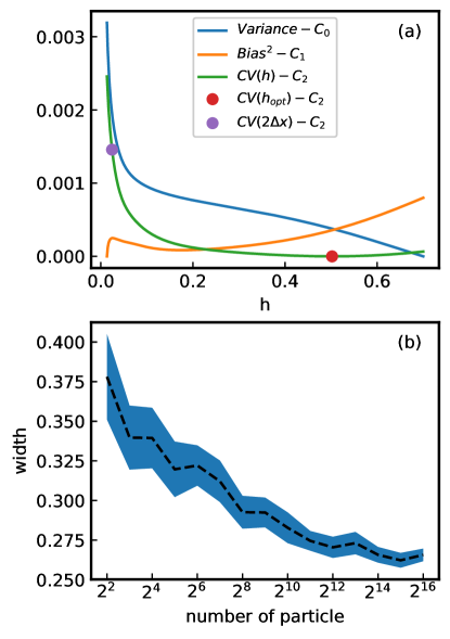
Figure 1: (a) The decomposition of the cross validation function. The blue curve and the orange curve indicate the variance and the bias squared term, respectively. The green curve is the total cross validation function. The purple dot and the red dot denote the $2\,dx$ for the standard PIC methods and the optimal width, respectively. (b) The relation between width and number of particles.The blue band is the 95% confidence interval with 20 ensembles and the dashed black curve is the mean.

To further reduce the MISE, adaptive width for each particle is calculated using the algorithms described in Section II.C. The density and electrical field at the initial time-step are shown in Fig. 2. The black dashed curve in Fig. 2a indicates the theoretical density function. The blue curve and the orange curve is estimated the density function using the standard PIC method and the KDE algorithm, respectively. The standard PIC method suffers from a large variance error. On the contrary, the KDE algorithm balances the variance and the bias error and results in a smooth curve near the the theoretical curve. The dashed black curve in Fig. 2b is the theoretical field. The blue curve and orange curve are the field obtained using the standard PIC method and the KDE algorithm, respectively. Even though the density is integrated to calculate the field, the standard PIC method still suffers from a large noise compared with the KDE algorithm using optimal width.

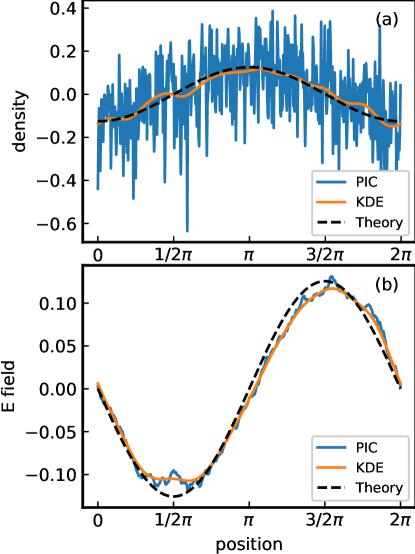
Figure 2: The density (a) estimated using the KDE algorithm (orange curve) and the standard PIC method (the blue curve), respectively. The black dashed curve is the theoretical density. The electric fields (b) calculated by the KDE algorithm (orange curve) and the standard PIC method (the blue curve), respectively. The black dashed curve is the theoretical electrical field.

The width is dynamically determined according to update algorithm described in Sec. II.D. The p-values of Anderson-Darling test is plotted in Fig. 3a. The width is updated at the time-steps in which p-values are less than the threshold and p-values decreases by half. Orange dots indicate the time-steps at which the widths are re-evaluated. In Fig. 3b, the width is plotted as a function of time.

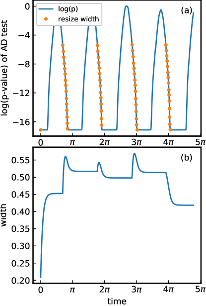
Figure 3: (a) The dynamics of log(p-values) of the Anderson-Darling test. The dots indicate the time-steps at which the optimal width is re-evaluated. (b) The width as a function of time according to the update algorithm.

Using the KDE algorithm, the Langmuir wave is simulated. The density and electric field at all time-steps are compared with those obtained using the standard PIC method in Fig. 4.

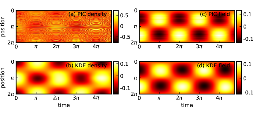
Figure 4: The density fluctuation of cold Langmuir wave as a function of time calculated by the standard PIC method (a) and the KDE algorithm (b). The electric field as a function of time calculated by the standard PIC method (c) and the KDE algorithm (d).

For this specific numerical example, the MISE can be calculated by definition according to Eq. (11), since the theoretical density is known. The MISE for density estimation using the standard PIC method is 0.1260, and that using the KDE algorithm is 0.0023. It is reduced by 98% using the KDE algorithm. Using the KDE algorithm leads to a 10% decrease in term of MISE from 0.112 to 0.101 compared to the standard PIC method.

The three noise reduction techniques, i.e., high order shape functions, kernel width optimization, and adaptive width adjustment can be applied combinatorially or individually. We have compared the noise reduction effects for different shape functions with and without kernel width optimizations using $2^{19}$ particles. The results are plotted in Fig. 5. In (a-d), for the first, second, third and fifth order shape functions with width $(order+1)\cdot dx$ as in standard PIC methods, the MISEs are $2.28031\times 10^{-3}$, $1.90144\times 10^{-3}$, $1.14667\times 10^{-3}$, and $0.74505\times 10^{-3}$ respectively. In (e), the von Mises shape is used with double grid width, and the MISE is $0.43698\times 10^{-3}$. In (f), by combining the first order shape with an optimized kernel width, the MISE is reduced to $0.17233\times 10^{-3}$. In (g), the von Mises shape with the optimized kernel width by the KDE method can reduce the MISE to $0.15423\times 10^{-3}$. And in (h), the von Mises shape with the optimal width by the adaptive KDE method further reduces the MISE to $0.13063\times 10^{-3}$.

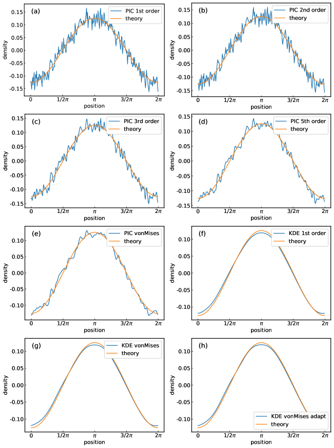
Figure 5: Noise reduction to different shape functions and kernel widths. In (a-d), the first, second, third and fifth order shape functions with width $(\text{order}+1)dx$ as in standard PIC method, (e) mixture of the von Mises shape with double grid width width as standard deviation, (f) mixture of the first order shape with optimized kernel width, (g) von Mises shape and optimized kernel width by the KDE method, and (h) the von Mises shape and optimal width by the adaptive KDE method.The Blue lines are the density estimations using each method and the orange lines are the theoretical results.

From these results we draw the following conclusions. Given the width of shape being $(\text{order}+1)\cdot dx$, the MISE decreases as the order of shape increases. The von Mises function is an infinitely differentiable function and can be viewed as an infinite order shape function. Hence it is the best estimator among all high order shape functions and reduces the MISE by 80.83%. But when using the optimal width, even the first order shape can reduce the MISE by 92.44%, outperforming all previous PIC methods. The noise reduction effects due to high order of shape functions and optimal kernel width are different. High order shape functions are aimed at reducing the bias. On the other hand, the optimized width method takes the variance into consideration and provides a smoother and more accurate density estimation. The combination of the von Mises shape function and optimal width can reduce the MISE by 93.23%. Finally, the adjusted width can further reduce MISE by 94.27%. The adjusted width effect will be significant when distribution functions contain sharp peaks and narrow valleys.

Performance of the three methods is also investigated from the viewpoint of computational cost. For comparison, we vary the number of simulation particles for different methods to achieve the same accuracy goal, which is chosen to be having an MISE less than $2.000\times 10^{-3}$. The computational time for different methods is measured and compared.

It is found that the standard PIC method requires $2^{19}$ particles to achieve an MISE of $1.997\times 10^{-3}$. The computation costs Central Processing Unit(CPU) time of 135 ms. The KDE method with the first order shape function requires only $2^{12}$ particles and MISE is $1.977\times 10^{-3}$. It runs for 81.3 ms. The KDE method with von Mises shape function requires $2^{12}$ particles as well and MISE is $1.949\times 10^{-3}$. But it needs 845 ms. According this result, the optimal strategy to achieve a given accuracy is to adopt the first order shape function and use the KDE to choose an optimal kernel width. Since the optimization to determine the optimal width is a fixed cost, it is more preferred to use KDE method in long-term simulations. This can then be neglected when averaged over each single time-step. The bottleneck using KDE method in parallel computation with Message Passing Interface(MPI) may hide in communication between processes since larger kernel length requires more data to exchange.

III.2 Linear Landau damping rate

When the electrons have a finite temperature, the Langmuir wave will be damped by the wave-particle interaction. This is the Landau damping Stix (1992). To simulate this phenomena, particles are drawn from an initial distribution which is perturbed in configuration space and Maxwellian with variance $\sigma_{v}^{2}$ in velocity space. One system consists of initial positions and velocities is call a ensemble. To do a fair comparison, the two methods should start from the same ensemble. With the same ensemble, we carry out simulations using the KDE algorithm and the standard PIC methods respectively.

In the simulation, the number of grid point is 256, the simulation time-step is 0.01, and $2^{15}$ particles are used. The initial velocity distribution is $f(v)=1/\sqrt{2\pi v_{th}^{2}}\exp[-v^{2}/(2v_{th}^{2})]$, where $v_{th}$ is the thermal velocity. The thermal velocity is normalized to $v_{th}=0.40$, which determines the spatial normalization. The initial density of electrons is uniform modulated by perturbation of the form $\rho_{1}=0.02\,\cos(1.0\,x)$. This simulation runs for 1500 steps.

For one specific ensemble, the density distribution with respect to time using the standard PIC method is plotted in Fig. 6a and result using the KDE algorithm is plotted in Fig. 6b. The electric field using the standard PIC method and the KDE algorithm are plotted in Fig. 6c and Fig. 6d, respectively. Compared with the standard PIC method, the KDE algorithm reduces the noise level on both the density and electrical field. This noise reduction is expected to render more accurate physical results. We now show that KDE algorithm generates a more accurate Landau damping rate.

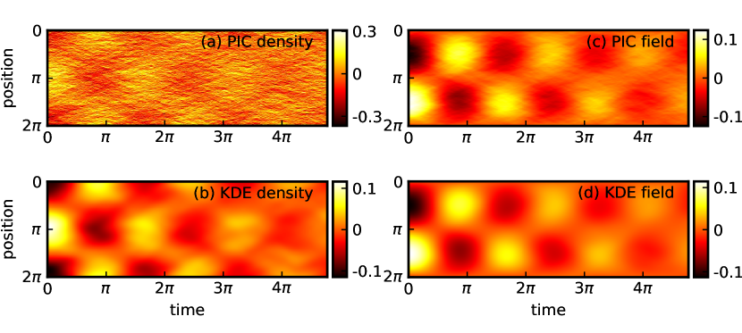
Figure 6: The density fluctuation of Landau damping as a function of time calculated by the standard PIC method (a) and the KDE algorithm (b). The electric field calculated by the standard PIC method (c) and the KDE algorithm (d). The normalized thermal velocity is $v_{th}=0.40$.

The Landau damping rate is calculated by the drop of energy of electric field. When the logarithm of electric energy is plotted, the slope of the line pass through the first two peaks after $t=0$ is assigned to be the damping rate. The logarithms of total electric field energy of this ensemble using the standard PIC method and the KDE algorithm are plotted in Fig. 7 with blue and red curves respectively. The energy peaks are marked by orange and purple dots. In this ensemble, theoretical damping rate is -0.096. Using the standard PIC method, the damping rate is -0.080, and the relative error is 16.4%. By contrast, using the KDE algorithm, the damping rate is -0.087, and the relative error is 9.4%.

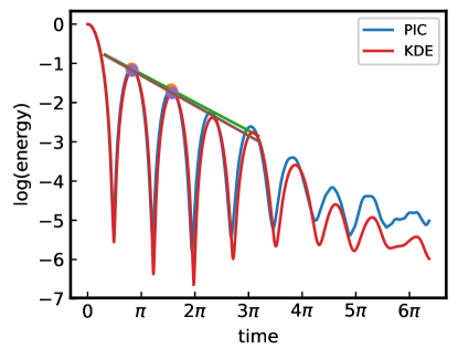
Figure 7: The logarithm of electric field energy as a function of time. The result using the standard PIC method (blue curve) is compared to that using the KDE algorithm (red curve).

However, comparison of the two methods on only one ensemble is not enough. To make the comparison more meaningful in statistical sense, the standard PIC method and the KDE method should be compared on the mean damping rate averaged over different ensembles corresponding to the same macroscopic state specified by plasma density, plasma temperature and velocity distribution. With the common random numbers variance reduction technique, we draw 30 different ensembles from the same distribution for both methods. The absolute error of the mean damping rate using the standard PIC method is 0.0113 with standard deviation of 0.0032, and the t-statistic is $t_{PIC}=3.82$. The absolute error of mean using the KDE algorithm is 0.0038 with standard deviation of 0.0034, and the t-static is $t_{KDE}=1.17$. At 95% confidence level, we cannot reject the null hypothesis that the damping rate obtained using the KDE algorithm is identical to the theoretical one. But the null hypothesis for the standard PIC method can be reject, that is to say, the damping rate from the standard PIC method deviates from theoretical result at 95% confidence level. Since the variace is reduced by the common random numbers technique, the null hypothesis that the error of the standard PIC method is the same as that of the KDE algorithm can be safely rejected at 95% confidence level. Therefore, we can draw the conclusion that the KDE algorithm improves the simulation result of the linear damping rate by reducing the noise level.

Next, we extend the results to different temperatures. We scan the thermal velocities from 0.20 to 0.45 for each step of 0.05. The results are plotted in Fig. 8a. The blue curve is the theoretical result, the green curve is the result using the KDE algorithm, and the orange is the that using the standard PIC method. It clear that KDE algorithm is closer to the theoretical values at every temperature. The numerical errors with error bar of 95% confidence interval is plotted in Fig. 8b, from which we can conclude that for each thermal velocity, the mean damping rate calculated by the KDE algorithm is more accurate than that calculated by the standard PIC method.

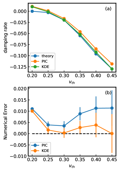
Figure 8: For the different thermal velocity, the simulations are run for 30 ensembles and the main damping rate is evaluated. The result using the KDE algorithm (green curve) is closer to the theoretical damping rate (blue curve) than that using the standard PIC method (orange curve) (a). The estimation error using the KDE algorithm (orange curve) and the standard PIC method (blue curve) are compared in (b). The 95% confidence intervals are plotted as error bar.

IV Conclusion And Discussion

In this paper, we proposed to use the Kernel Density Estimation (KDE) algorithm to reduce the noise for Particle-In-Cell (PIC) simulations. A framework for quantitatively evaluating and minimizing the error of density estimation for PIC simulations is established using the KDE theory. Under this framework, the error on particle density estimation for PIC algorithms, as measured by the Mean Integrated Square Error (MISE), consists of two parts, the bias error and the variance error. The bias error is the systematic error and the variance error is the familiar noise in PIC simulations. A careful analysis showed that the error on particle density estimation in the standard PIC methods is dominated by the variance error, which is consistent with well-known fact that PIC simulations suffer from large noise. Analysis also suggested that the noise level and total MISE can be significantly reduced by increasing the width of the kernel function, i.e., particle shape function. In the KDE algorithm developed in the present study, an optimal width is obtained by minimizing the MISE, represented by a Cross-Validation (CV) function, which is constructed using the leave-one-out estimation. The algorithm is further improved by adopting a particle-wise width optimization scheme. For the dynamics of the PIC systems, an efficient width update algorithm is also developed. To test the KDE algorithm, we carried out simulations study of the Langmuir wave and its Landau damping. Simulation results showed that relative to the standard PIC methods, the KDE algorithm can reduce the noise level on density estimation by 98%, and give a much more accurate result on the linear damping rate.

The next step of the research will mainly focus on the choice of different loss functions and optimization techniques. The utility of the MISE loss function has clear statistical meaning, i.e., it consists of the bias and the variance, moreover, the choice of loss function can be and has been extended to a wide range in the field of machine learning. Using the $L_{1}$ norm will enhance locality and improve the robustness for outliers. The cross entropy with leave one out estimation is another alternative. Furthermore, a more complex KDE method can be constructed to model the joined distribution of positions and velocities. The loss functions will not only measure the variance and bias of position, but also those of phase space as a whole. It will punish particles with outlier velocities as well. New optimization method, such as the SGD (stochastic gradient descent) method Friedman et al. (2001) will be explored to accelerate the optimal width algorithm without sacrificing accuracy.

Recently, structure-preserving geometric algorithms for plasma physics have been actively studied [28-35]. This new class of algorithms are designed to preserve the geometric structure of physical systems and bound globally for all simulation time-steps the errors on energy, momentum, etc. We plan to combine the KDE method with these the structure-preserving geometric algorithms to future improve the performance and accuracy of PIC simulations.

Though the density error is improved by  98% than the standard PIC method, the field error is only improved by  10%. The field is the integration of density function, and thus smoother than the density function. Nevertheless, it is valuable to have an effective tool for noise reduction on the density. There are physical situations, such as in turbulence transport, when the density fluctuation is important. On the other hand, to further improve the accuracy for the field, we can adopt a loss function to model the error of the field and perform optimization, which will be investigated in future studies.

Appendix A Leave-one-out Necessity

In this appendix, we prove the fact that $h=0$ minimizes the the KDE estimator defined by Eq. (3). In this case, the CV function is

$$CV(h) =\int\hat{f}(x)^{2}\,dx-2E[\hat{E}_{X}[\hat{f}(X)]]$$ (30)

$$=\frac{1}{n^{2}h}\sum_{i=1}^{n}\sum_{j=1}\bar{K}\left(\frac{X_{i}-X_{j}}{h}\right)$$

$$\qquad-\frac{2}{n^{2}h}\sum_{i=1}^{n}\sum_{j=1}^{n}K\left(\frac{X_{i}-X_{j}}{h}\right).$$ (31)

By extracting the terms with $i=j$, the CV function is rearranged into

$$CV(h) =\frac{1}{nh}\left(\bar{K}(0)-2K(0)\right)$$

$$\quad+\frac{1}{n^{2}h}\sum_{i=1}^{n}\sum_{j\neq i,j=1}^{n}\left[\bar{K}\left(\frac{X_{i}-X_{j}}{h}\right)-2K\left(\frac{X_{i}-X_{j}}{h}\right)\right].$$ (32)

Minimizing the MISE is equivalent to minimizing $E[CV(h)]$. We now investigate how the expectation of the CV function depends on the width $h$. First, we look at the expectation of kernel function,

$$E\left[K\left(\frac{X_{i}-x}{h}\right)\right] =\int f(\xi)K\left(\frac{\xi-x}{h}\right)\,d\xi$$ (33)

$$=\int f(x+h\eta)K(\eta)hd\eta$$ (34)

$$=h\int\left[f(x)+f^{\prime}(x)h\eta+\frac{1}{2}f^{\prime\prime}(x)h^{2}\eta^{2}+O(h^{3})\right]K(\eta)\,d\eta$$ (35)

$$=h\left[f(x)+\frac{h^{2}\kappa_{2}}{2}f^{\prime\prime}(x)+\frac{h^{4}\kappa_{4}}{4!}f^{(4)}(x)+O(h^{6})\right],$$ (36)

where $\kappa_{2}=\int\eta^{2}K(\eta)\,d\eta$ and $\kappa_{4}=\int\eta^{4}K(\eta)\,d\eta$ are constants depending only on the kernel.

Now we look at each term in the second part of CV function. Since $X_{i}$ and $X_{j}$ are independent, the first term is

$$E\left[\bar{K}\left(\frac{X_{i}-X_{j}}{h}\right)\right] =\frac{1}{h}E\int K\left(\frac{X_{i}-x}{h}\right)K\left(\frac{X_{j}-x}{h}\right)\,dx$$ (37)

$$=\frac{1}{h}\int E\left[K\left(\frac{X_{i}-x}{h}\right)\right]E\left[K\left(\frac{X_{j}-x}{h}\right)\right]\,dx$$ (38)

$$=\frac{1}{h}\int E\left[K\left(\frac{X_{i}-x}{h}\right)\right]^{2}\,dx$$ (39)

$$=h\int\left[f(x)+\frac{h^{2}\kappa_{2}}{2}f^{\prime\prime}(x)+\frac{h^{4}\kappa_{4}}{4!}f^{(4)}(x)\right]^{2}\,dx.$$ (40)

The second term is

$$E\left[K\left(\frac{X_{i}-X_{j}}{h}\right)\right] =\int f(x)dx\int K\left(\frac{\xi-x}{h}\right)f(\xi)d\xi$$ (41)

$$=h\int f(x)\left[f(x)+\frac{h^{2}\kappa_{2}}{2}f^{\prime\prime}(x)+\frac{h^{4}\kappa_{4}}{4!}f^{(4)}(x)\right]\,dx,$$ (42)

Therefore, the leading terms for the CV function are

$$CV(f)=\frac{1}{nh}\left(\bar{K}(0)-2K(0)\right)+h^{4}\frac{\kappa_{2}^{2}(n-1)}{4n}\int\left[f^{\prime\prime}(x)\right]^{2}\,dx-\frac{n-1}{n}\int f(x)^{2}dx+O(h^{5}).$$ (43)

Assuming that the kernel function has peak at $x=0$ such that for all $x$, $K(0)\geq K(x)$, which is the case for the von Mises distribution, we have

$$\bar{K}(0)-2K(0) =\int K(x)^{2}\,dx-2K(0)$$ (44)

$$\leq\int K(0)K(x)\,dx-2K(0)$$ (45)

$$=K(0)-2K(0)<0.$$ (46)

Meanwhile,

$$\frac{\kappa_{2}^{2}}{4}\int\left[f^{\prime\prime}(x)\right]^{2}\,dx>0.$$ (47)

It is thus straightforward to show that the the CV function goes to $-\infty$ when $h\to 0$. This proves the fact that $h=0$ minimizes the KDE estimator defined by Eq. (3).