Oscillating red giants in eclipsing binary systems: empirical reference value for asteroseismic scaling relation

Abstract

The internal structures and properties of oscillating red-giant stars can be accurately inferred through their global oscillation modes (asteroseismology). Based on 1460 days of Kepler observations we perform a thorough asteroseismic study to probe the stellar parameters and evolutionary stages of three red giants in eclipsing binary systems. We present the first detailed analysis of individual oscillation modes of the red-giant components of KIC 8410637, KIC 5640750 and KIC 9540226. We obtain estimates of their asteroseismic masses, radii, mean densities and logarithmic surface gravities by using the asteroseismic scaling relations as well as grid-based modelling. As these red giants are in double-lined eclipsing binaries, it is possible to derive their independent dynamical masses and radii from the orbital solution and compare it with the seismically inferred values. For KIC 5640750 we compute the first spectroscopic orbit based on both components of this system. We use high-resolution spectroscopic data and light curves of the three systems to determine up-to-date values of the dynamical stellar parameters. With our comprehensive set of stellar parameters we explore consistencies between binary analysis and asteroseismic methods, and test the reliability of the well-known scaling relations. For the three red giants under study, we find agreement between dynamical and asteroseismic stellar parameters in cases where the asteroseismic methods account for metallicity, temperature and mass dependence as well as surface effects. We are able to attain agreement from the scaling laws in all three systems if we use $\Delta\nu_{\rm ref,emp}=130.8\pm 0.9\,\mu$Hz instead of the usual solar reference value.

1 Introduction

Asteroseismology is the study of stellar oscillations with the aim of unravelling the structure and dynamics of stellar interiors. In-depth asteroseismic studies require either high-precision photometric time-series observations or time series of accurate radial velocity measurements (RVs). The former has been obtained by space missions such as MOST (e.g. Barban et al., 2007; Kallinger et al., 2008), CoRoT (e.g. Baglin et al., 2007; De Ridder et al., 2009) and Kepler (e.g. Borucki et al., 2010). From 2009 to 2013, the nominal Kepler mission provided nearly continuous photometric time-series data for more than $100\,000$ stars. These data are suitable for asteroseismic analyses and led to many discoveries in the field of red-giant seismology: determination of evolutionary stages (e.g. Bedding et al., 2011; Mosser et al., 2014; Elsworth et al., 2017), rotation studies (e.g. Beck et al., 2012; Mosser et al., 2012b), stellar parameter determinations (Kallinger et al., 2010; Huber et al., 2010; Hekker et al., 2013b), ensemble studies and galactic archaeology (e.g. Corsaro et al., 2012; Miglio et al., 2013; Casagrande et al., 2016), amongst others. For recent overviews see Hekker (2013) and Hekker & Christensen-Dalsgaard (2017).

Pulsating red giants exhibit solar-like oscillations that are driven by the turbulent convection in the stellar envelope. The physical properties of red giants, such as mean density and surface gravity and thus stellar mass and radius, can be determined through the study of their oscillations. The most commonly used asteroseismic method is based on scaling relations (e.g. Ulrich, 1986; Brown et al., 1991; Kjeldsen & Bedding, 1995) that use direct observables from the oscillation spectrum as input. These so-called global oscillation parameters can be measured in a large number of red giants for which high-precision photometric data are available. However, the asteroseismic scaling relations assume that all stars have an internal structure homologous to the Sun (e.g. Belkacem et al., 2013). Since evolved G and K giants span a wide range of masses, metallicities and evolutionary stages different than that of the Sun, the validity of these scaling relations, based on the principle of homology to the Sun, has to be tested. One possibility is to use eclipsing binary systems with a pulsating red-giant component. For double-lined eclipsing binaries, the stellar mass and radius of the red-giant component can be derived independently of asteroseismology through the binary orbit analysis using Kepler’s laws. The binary analysis is limited to the cases in which the orbital parameters can be resolved and require spectra covering the full orbital period of the system.

So far a number of eclipsing binary systems with a red-giant component were detected in Kepler data (e.g. Hekker et al., 2010; Gaulme et al., 2013). The first such system, KIC 8410637, was identified by Hekker et al. (2010), who carried out a preliminary asteroseismic study based on a month long photometric time series of data in which only one eclipse was detected. The stellar parameters of the red-giant star could be measured from both the solar-like oscillations and from spectroscopy. A detailed comparison between the asteroseismic and dynamical stellar mass and radius of the red giant was performed by Frandsen et al. (2013), who found agreement between the binary and asteroseismic results within uncertainties. When Huber (2014) repeated the asteroseismic analysis of KIC 8410637 with a longer Kepler dataset, he contested the findings of Frandsen et al. (2013) and reported large discrepancies between the asteroseismic and dynamical stellar parameters.

Beck et al. (2014) carried out a seismic and binary analysis of 18 red-giant stars among which was KIC 9540226. The red giant was not only found to be in an eccentric eclipsing binary, but also to exhibit an increase in flux during the actual periastron passage (Kumar et al., 1995; Remus et al., 2012). These stars are colloquially referred to as “heartbeat stars” (Thompson et al., 2012). Beck et al. calculated the orbital parameters of the system from high-resolution spectroscopy and estimated the stellar parameters of the red giant from the asteroseismic scaling relations. In a more recent study, the mass and the radius of the red-giant component of KIC 9540226 could be constrained from two consecutive binary analyses (Brogaard et al., 2016, 2018). Moreover, Brogaard et al. (2018) computed several estimates of its asteroseismic mass and radius based on different methodologies and by using the asteroseismic observables presented by Gaulme et al. (2016).

KIC 8410637, KIC 5640750 and KIC 9540226 were also part of several ensemble studies (Gaulme et al., 2013, 2014; Gaulme et al., 2016, hereafter G16). In these surveys, eclipse modelling and modelling of the radial velocities were used to derive the orbital and dynamical stellar parameters. In addition, masses and radii of the red-giant components were computed by using the asteroseismic scaling relations. In an extensive comparison between the results from detailed binary modelling and asteroseismology, they showed that the stellar masses and radii are systematically overestimated when the asteroseismic scaling relations are used.

In Table 1 we summarize the orbital and stellar parameters for the three red-giant stars (KIC 8410637, KIC 5640750 and KIC 9540226) that are the subject of this study.

For a number of red-giant components in eclipsing binary systems it has been found that the dynamical and asteroseismic stellar parameters differ significantly. This leads us to investigate three such systems in detail, both from the binary point of view including a dedicated spectral disentangling analysis as well as by obtaining individual frequencies. In addition to the observational analysis, we use an asteroseismic grid-based approach to model the three red-giant components. KIC 8410637, KIC 5640750, and KIC 9540226 belong to wide eclipsing binary systems where the components are not expected to be strongly influenced by tidal effects and/or mass transfer. All three systems were observed during the nominal four year long Kepler mission providing a large photometric dataset of unprecedented accuracy and supplemented with additional high-resolution spectra from ground-based observatories. We analyze these spectroscopic and photometric data and derive up-to-date values of the stellar parameters from both the asteroseismic and orbital analysis. Since the stellar parameters determined using Kepler’s laws are considered to be both accurate and precise, they provide a means to test the reliability of the asteroseismic mass and radius from the scaling laws.

For the current in-depth study we obtained orbital solutions and physical properties of three eclipsing binary systems from Kepler light curves and phase-resolved spectroscopy (Section 2). In addition, we analyzed the Fourier spectra of the red-giant components in these systems to derive both global oscillation parameters as well as individual frequencies (Section 3.3). We studied their asteroseismic stellar parameters and evolutionary states (Section 3.4). In Section 4 we discuss and compare stellar parameters obtained from different asteroseismic methods and from the binary orbit. In the same section we provide an overview of tests that we performed to investigate the importance of different observables that are used for the determination of the asteroseismic stellar parameters and we present the conclusions of our study in Section 5.

Table 1: Stellar and orbital parameters of the red giants studied here obtained from the literature (as per the rightmost column). The orbital periods ($P$) and eccentricities ($e$) are determined from orbital analysis of these binary systems. Stellar parameters ($M,R,\log g$) are based on either asteroseismic scaling relations or binary analysis. The latter are indicated with asterisks. Effective temperatures ($T_{\rm eff}$) and logarithmic surface gravities ($\log g$) are mostly derived from spectra within the study referred to. We indicate the cases where they were adopted from the original (^a, Brown et al., 2011) and revised (^b, Huber et al., 2014) Kepler input catalogs (KIC).

$P$ [days]	$e$	$R$ [$\rm R_{\odot}$]	$M$ [$\rm M_{\odot}$]	$\log g$	$T_{\rm eff}$ [K]	Evol. phase	Publication
KIC 8410637
$>75$		$11.80\pm 0.60$	$1.70\pm 0.30$	$2.700\pm 0.150$	$4650\pm 80$		Hekker et al. (2010)
$408.32$	$0.69$	$10.74\pm 0.11$*	$1.56\pm 0.03$*	$2.569\pm 0.009$*	$4800\pm 80$	RC	Frandsen et al. (2013)
		$11.58\pm 0.30$	$1.83\pm 0.14$	$2.572\pm 0.011$	$4800\pm 80$		Huber (2014)
$408.32$	$0.69$	$11.01\pm 0.26$	$1.61\pm 0.11$	$2.760\pm 0.400$b	$4872\pm 139$b	RC	Gaulme et al. (2014)
		$11.20\pm 0.20$	$1.70\pm 0.07$	$2.569\pm 0.005$	$4800\pm 100$		G16seis
		$10.75\pm 0.20$	$1.51\pm 0.07$	$2.555\pm 0.005$	$4605\pm 80$	RGB	This workseis
408.32	0.686	$10.60\pm 0.05$*	$1.47\pm 0.02$*	$2.556\pm 0.003$*	$4605\pm 80$		This workdyn
KIC 5640750
$987.40$	$0.32$	$14.27\pm 0.31$	$1.45\pm 0.09$	$2.561\pm 0.400$b	$4727\pm 142$b	RGB/AGB	Gaulme et al. (2014)
		$13.08\pm 0.26$	$1.15\pm 0.06$	$2.267\pm 0.005$	$4525\pm 75$	RGB	This workseis
987.40	0.323	$13.12\pm 0.09$*	$1.16\pm 0.01$*	$2.266\pm 0.006$*	$4525\pm 75$		This workdyn
KIC 9540226
$175.43$	$0.39$	$14.10\pm 0.30$	$1.60\pm 0.10$	$2.370\pm 0.010$	$4600\pm 150$a	RGB	Beck et al. (2014)
$175.46$	$0.39$	$14.01\pm 0.26$	$1.59\pm 0.08$	$2.346\pm 0.030$b	$4761\pm 143$b	RGB	Gaulme et al. (2014)
		$13.60\pm 0.20$	$1.45\pm 0.05$	$2.334\pm 0.004$	$4692\pm 65$		G16seis
$175.44$	$0.388$	$12.80\pm 0.10$*	$1.33\pm 0.05$*	$2.349\pm 0.008$*	$4692\pm 65$		G16dyn
		$13.06\pm 0.16$*	$1.38\pm 0.04$*	$2.345\pm 0.010$*	$4680\pm 80$		Brogaard et al. (2018)
		$12.94\pm 0.25$	$1.26\pm 0.06$	$2.314\pm 0.006$	$4585\pm 75$	RGB	This workseis
175.44	0.388	$13.43\pm 0.17$*	$1.39\pm 0.03$*	$2.326\pm 0.010$*	$4585\pm 75$		This workdyn

2 Physical properties of the systems from light curves and radial velocity time series

2.1 Kepler light curves and ground-based spectroscopic data

For the eclipse modelling, we extracted the light curves of each eclipse from the Kepler datasets. In this case, we retained all data obtained within three eclipse durations of the eclipse. The data were then converted from flux to magnitude units and a low-order polynomial was fitted to normalise the out-of-transit data to zero relative magnitude. This step removes any slow trends due to instrumental effects and stellar activity. We tested the effects of different treatment of the light curve normalisation (e.g. polynomial order), and found that it does not have a significant impact on the best-fitting parameters.

By definition the primary eclipse is deeper than the secondary eclipse, and occurs when the hotter star is eclipsed by the cooler star. For all three objects, the dwarf star is smaller and hotter than the giant, so the primary eclipse is an occultation and the secondary eclipse is a transit. This also means that according to standard terminology (e.g. Hilditch, 2001) the dwarf is the primary star and the giant is the secondary star. To avoid possible confusion, we instead refer to the stellar components as the “dwarf” (denoted as A) and “giant” (denoted as B).

Complementary to Kepler photometry we use spectroscopic data for the binary systems KIC 8410637, KIC 5640750 and KIC 9540226, which were obtained with the Hermes spectrograph (Raskin et al., 2011; Raskin, 2011) mounted on the 1.2m Mercator telescope in La Palma, Canary Islands, Spain. These spectra cover the wavelength range from $3\,750-9\,000\,\AA$ with a resolution of $R\simeq 85\,000$. Emission spectra of thorium-argon-neon reference lamps are provided in close proximity to each exposure to allow the most accurate wavelength calibration of the spectra possible. Some Hermes spectra for KIC 8410637 and KIC 9540226 were already used in previous studies by Frandsen et al. (2013) and Beck et al. (2014). Observations were continued to extend the number of spectra and time base of the spectroscopic data. Moreover, the long-period system KIC 5640750 has been monitored spectroscopically by members of our team since its discovery as a binary.

2.2 Spectroscopic orbital elements from cross-correlation function and spectral disentangling

2.2.1 Cross-correlation function (ccf)

For the three red giants under study we reanalyzed the archived Hermes data and obtained radial velocities by using the cross-correlation method (e.g. Tonry & Davis, 1979). Based on this approach each wavelength-calibrated spectrum in the range from $4\,780-6\,530\,\AA$ was cross-correlated with a line mask optimized for Hermes spectra (Raskin et al., 2011). In this case a red-giant-star template was used that contains spectral lines corresponding to the spectrum of Arcturus. This method provides excellent precision for deriving the RVs of red-giant stars showing solar-like oscillations (Beck et al., 2014). For KIC 8410637 those RVs with large measurement uncertainties were not included in the further analysis. This leaves 43 RVs for the giant, with a root mean square ($rms$) scatter of 0.23 km s^-1 around the best fit, and 20 for the dwarf with a scatter of 0.92 km s^-1 (Table 11). In the case of KIC 5640750 we only have RV data of the giant star (22 observations with a scatter of 0.08 km s^-1, Table 12), since we were not able to detect the signature of the dwarf component with ccf. As a further attempt to obtain its RVs we applied the least-squares deconvolution (LSD) method developed by Tkachenko et al. (2013). This technique is similar to a cross-correlation with a set of $\delta$ functions. It is sensitive to small contributions and thus more suitable for the detection of faint components in double-lined spectroscopic binary systems. Although the overall signal-to-noise ratio (S/N) was high, the contribution from the dwarf star was very weak and therefore difficult to detect. With LSD we were not able to measure sufficiently precise RVs for the dwarf component that could be used to further constrain the orbital parameters for the system KIC 5640750. For KIC 9540226 we derived 32 RVs for the giant with a scatter of 0.33 km s^-1 that we present in Table 13. These were supplemented by RV data for the dwarf star recently published by Gaulme et al. (2016) (7 RVs with a scatter of 0.91 km s^-1).

Based on the radial velocities determined for the stars in these binary systems we obtained orbital elements by using Kepler’s laws. The lack of RVs for the dwarf star of KIC 5640750 means we cannot measure the masses and radii of the component stars without additional constraints. As these parameters are important for our current study, we extended the spectroscopic analysis to detect the dwarf component of KIC 5640750 by using spectral disentangling.

Table 2: Spectroscopic orbital elements for KIC 8410637 (columns 2–3), KIC 5640750 (columns 4–6) and KIC 9540226 (columns 7–8) determined using cross-correlation (ccf) and spectral disentangling (spd). We adopted the solutions based on spd in the further analysis of these eclipsing binary systems. See Section 2.2.3 for parameter definitions. We note that $T_{0}$ is given in heliocentric julian date (HJD).

Parameter	KIC 8410637				KIC 5640750						KIC 9540226
	ccf		spd		ccf		spd 1		spd 2		ccf		spd
$P$ [d]	408.3248	$\pm$ 0.0004	-		987.398	$\pm$ 0.006	-		-		175.4438	$\pm$ 0.0008	-
$T_{0}$ [d]	398.9449	$\pm$ 0.0007	403.53	$\pm$ 0.06	269.215	$\pm$ 0.004	188.7	$\pm$ 1.1	188.5	$\pm$ 1.1	817.289	$\pm$ 0.002	841.71	$\pm$ 0.08
$e$	0.686	$\pm$ 0.001	0.694	$\pm$ 0.004	0.326	$\pm$ 0.002	0.323	$\pm$ 0.008	0.322	$\pm$ 0.008	0.3877	$\pm$ 0.0003	0.387	$\pm$ 0.003
$\omega$ [deg]	120.9	$\pm$ 0.1	120.7	$\pm$ 0.2	34.3	$\pm$ 0.7	34.0	$\pm$ 0.7	33.6	$\pm$ 0.7	183.5	$\pm$ 0.6	184.2	$\pm$ 0.7
$K_{\rm A}$ [km s-1]	30.33	$\pm$ 0.22	29.37	$\pm$ 0.12	-		17.21	$\pm$ 0.18	15.10	$\pm$ 0.19	31.48	$\pm$ 0.40	31.94	$\pm$ 0.32
$K_{\rm B}$ [km s-1]	25.76	$\pm$ 0.09	26.13	$\pm$ 0.08	14.64	$\pm$ 0.03	14.68	$\pm$ 0.05	14.66	$\pm$ 0.06	23.24	$\pm$ 0.21	23.33	$\pm$ 0.14
$q$	0.849	$\pm$ 0.008	0.890	$\pm$ 0.005	-		0.853	$\pm$ 0.011	0.971	$\pm$ 0.012	0.738	$\pm$ 0.016	0.730	$\pm$ 0.032

2.2.2 Spectral disentangling (spd)

The spectra of the binary stars under study are dominated by the spectra of the red-giant components since they contribute the prevailing fraction of the total light of the systems. From the light curve analysis (see light ratio between components in Table 3, Section 2.3) it was found that the dwarf companions contribute only about 9.2, 6.5, and 2.0 per cent to the total light of the system for KIC 8410637, KIC 5640750, and KIC 9540226, respectively. This makes the RVs of the Doppler shifts of the faint companions more difficult to detect, i.e. the $rms$ scatter of the dwarfs is about three times more uncertain than for the giants for KIC 8410637 and KIC 9540226 and undetectable for KIC 5640750. The spectral lines of both components are, however, present in the spectra and to extract both we apply spectral disentangling (spd).

The method of spd was developed by Simon & Sturm (1994). In this method, the individual spectra of the components as well as a set of orbital elements can be optimised simultaneously. During this process the fluxes of the observed spectra are effectively co-added. This results in disentangled spectra that have a higher S/N compared to the observed spectra. There is no need for template spectra like in the cross-correlation method. This is highly beneficial in the case of barely visible components’ spectrum, like in our case (see Mayer et al., 2013; Torres et al., 2014; Kolbas et al., 2015, for other examples). With the method of spd the spectra of the faint dwarf companions were successfully reconstructed with the fractional light in the visual spectral region at the extreme values of barely $\sim 1-2$ per cent.

For the present work, we used the spectral disentangling code fdbinary (Ilijic et al., 2004), which operates in Fourier space based on the prescription of Hadrava (1995) including some numerical improvements. In particular, the Discrete Fourier Transform is implemented in fdbinary, which gives more flexibility in selecting spectral segments for spd while still keeping the original spectral resolution. We used the wavelength range of the spectra from $5\,000-6\,000\,\AA$ for both the determination of the orbital elements and the isolation of the individual spectra of the components.

In fdbinary the optimisation is performed with a simplex routine (cf. Press et al., 1989). We performed 100 runs, each with 1000 iterations, examing a relatively wide parameter space around an initial set of parameters. In most cases of high S/N spectra, that are well distributed in the orbital phases, the convergence is achieved quite fast. The uncertainties in the determination of the orbital elements were then calculated with a novel approach using a bootstrapping method (Pavlovski et al. in prep.). The faint companion’s spectra for all three systems were extracted (see Figures 1 and 2).

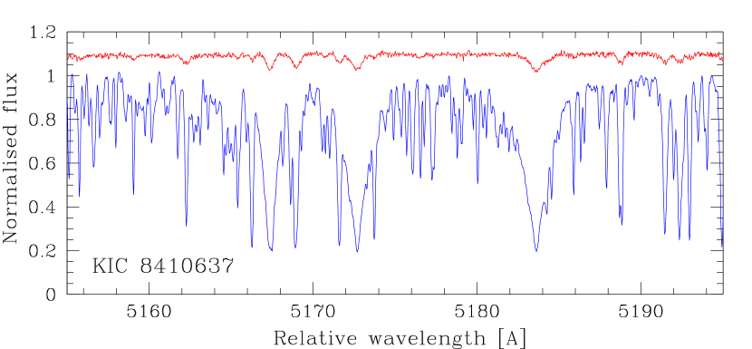
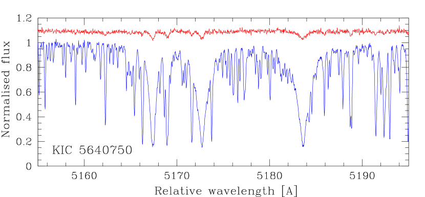
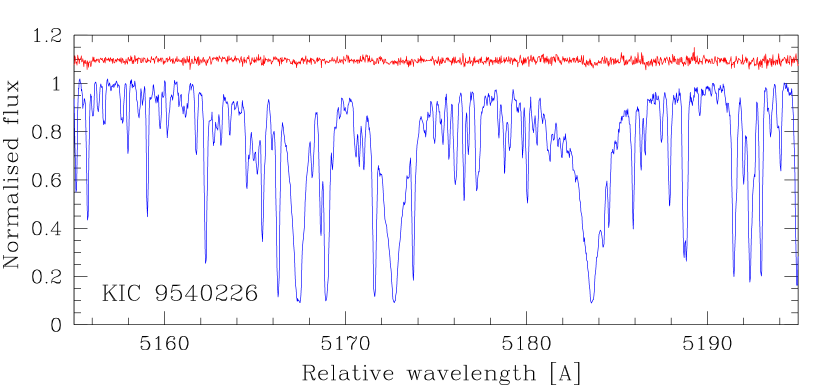
Figure 1: Disentangled spectra for the giant (blue) and dwarf (red) component of the eclipsing binary systems KIC 8410637 (top panel), KIC 5640750 (middle), and KIC 9540226 (bottom) centered on Mg i triplet at $\lambda=5168-5185$ Å. The spectra are normalized with respect to the composite continuum and for better visibility we use an arbitrary offset between the individual spectra of the binary components.

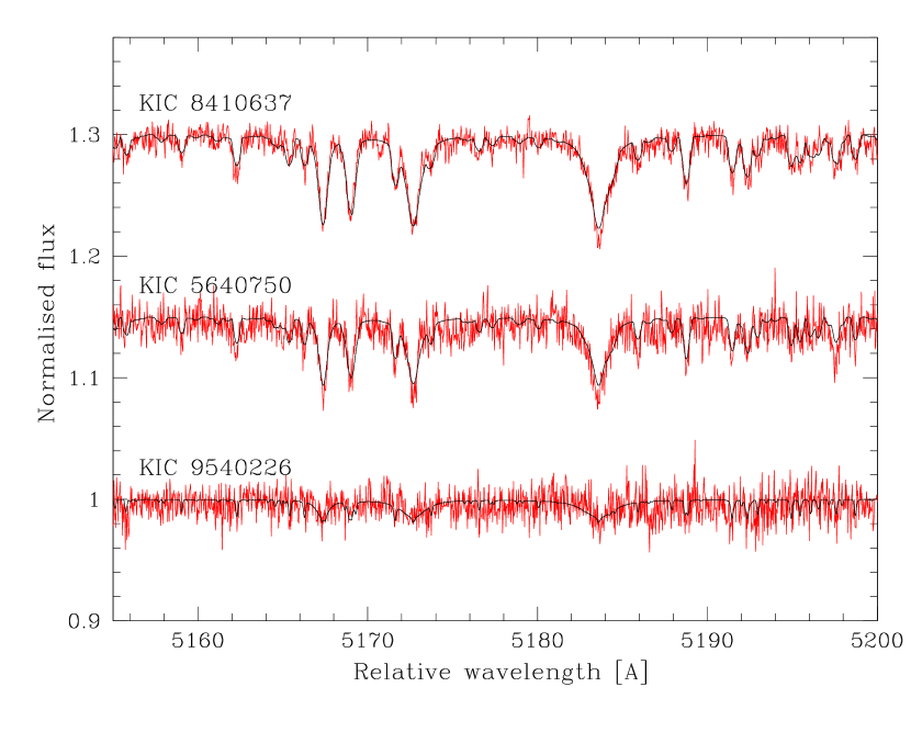
Figure 2: Close-ups of the disentangled spectra for the dwarf components (red) of the eclipsing binary systems KIC 8410637 (top panel), KIC 5640750 (middle), and KIC 9540226 (bottom) centered on Mg i triplet at $\lambda=5168-5185$ Å. Synthetic spectra are over-plotted in black. The spectra are normalized with respect to the composite continuum and for better visibility we use an arbitrary offset between the individual spectra of the dwarf components.

2.2.3 Orbital elements

For the three binary systems under study we report the spectroscopic orbital elements obtained from ccf and spd analysis in Table 2. These include the orbital period $P$, the time of periastron $T_{0}$, the eccentricity $e$, the longitude of periastron $\omega$, the radial velocity semi-amplitudes of the dwarf and giant component $K_{\rm A}$, $K_{\rm B}$ and the mass ratio $q=K_{\rm A}/K_{\rm B}$. The comparison of the results shows agreement between both methods. We note, however, that $T_{0}$ is different from spd and ccf for KIC 5640750 since about one third of the orbital phase is not covered by spectroscopic observations, which results in ambiguities regarding its orbital parameters (Figure 4). From spd we derived RV semi-amplitudes for all components in the three binary systems making the determination of the dynamical masses for all stars possible. Hence, we adopted these solutions for the further analysis.

KIC 5640750: In the current study we present the first spectroscopic orbit for this binary system based on both components. The ccf nor LSD analysis did reveal the radial velocities of the dwarf spectrum. According to our light curve analysis (Section 2.3) the companion star contributes only $\sim 6.5$ per cent to the total light in the visual passband. In addition, the long orbital period of 987 days makes the detection of the dwarf spectrum difficult since for such small Doppler shifts the spectral lines are along the whole cycle close to the prominent lines of the red-giant component. From the spd analysis we find two statistically significant solutions for this system which are indistinguishable and whose difference is barely visible in the disentangled spectra. This ambiguity arises due to an insufficient coverage of the orbital phase which lacks spectroscopic observations between 0 and 0.35 (see bottom left in Figure 4). Thus, only one extremum in the RV curve is covered by spectroscopic observations. As a result we obtain more than one local minimum in the spd analysis due to spurious patterns in the reconstructed spectra of the individual components, which can also affect the quality of the orbital solution (Hensberge et al., 2008). As a further attempt to lift the ambiguity between the two orbital solutions, we rerun the spd with fixed $e$ and $\omega$ without success. In any case, follow-up observations would be required to resolve this ambiguity by filling the gap in the orbital phases. In the current study, we use both solutions of this system to infer the stellar parameters of its components and we check these results for consistencies with asteroseismic stellar parameters. It should be noted that the RV semi-amplitudes for the giant are within 1$\sigma$ confidence level for all solutions.

KIC 8410637: In a comprehensive study by Frandsen et al. (2013) the first spectroscopic orbit was determined for this binary system. Even with about 10 per cent contribution to the total light, the dwarf companion is barely detectable due to a long orbital period of $P\sim 408$ days. Frandsen et al. used several methods to measure the radial velocities for both components; the line broadening function (Rucinski, 2002), the two-dimensional cross-correlation (2D-ccf, Zucker & Mazeh, 1994), and the Fourier spectral disentangling (Hadrava, 1995). These three sets of measurements gave consistent orbital parameters within 1$\sigma$ errors. Their final orbital solution is a mean of the results determined from the line broadening function and 2D-ccf, and reads, $K_{\rm A}=30.17\pm 0.39$  km s^-1, and $K_{\rm B}=25.85\pm 0.07$  km s^-1, with the mass ratio, $q=0.857\pm 0.011$. Comparing Frandsen et al. spectroscopic solution with our ccf and spd results, the agreement is only at a 3$\sigma$ confidence level for the RV semi-amplitudes, and at a 1$\sigma$ level for the geometric orbital parameters, i.e. the eccentricity, and the longitude of periastron. It is difficult to trace the source of these differences. Some systematics could arise because of the different methodology and different datasets that were used. Frandsen et al. worked with three spectroscopic datasets that were collected with different spectrographs of comparable spectral resolution, fies at the Nordic Optical Telescope, Hermes at the Mercator Telescope, and ces at the Thüringer Landessternwarte. We used Hermes spectra exclusively, hence our dataset is homogeneous, yet less extensive. Since there is no need for template spectra in the spd technique, this method is not liable to mismatch problems as the methods used by Frandsen et al. (2013), as shown in numerical experiments by Hensberge & Pavlovski (2007).

KIC 9540226: The first attempt to determine the spectroscopic orbit for this binary system was made by Beck et al. (2014). The cross-correlation method applied on 31 Hermes spectra did not reveal the dwarf’s spectrum. Hence, only the giant’s RV semi-amplitude was determined, $K_{\rm B}=23.32\pm 0.04$  km s^-1, and the geometric orbital parameters, the eccentricity $e=0.39\pm 0.01$, and the longitude of periastron $\omega=4.0\pm 0.6$ deg. The Kepler light curve solution published by Gaulme et al. (2016) shows that the dwarf component contributes barely $\sim 2$ per cent to the total light. Despite the low secondary contribution to the total flux, Gaulme et al. report a detection of the dwarf spectra in 7 out of 12 of their observations by using ccf. They used a new series of spectra secured with the 3.5m ARC telescope at Apache Point Observatory. It is encouraging that the spectroscopic orbital elements derived by Gaulme et al. (2016) and ours based on spd (Table 2) agree within 1$\sigma$ uncertainties.

2.2.4 Individual components’ spectra from spd

Spectral disentangling was performed in pure “separation” mode (Pavlovski & Hensberge, 2010) since the light curves do not show any significant light variations outside the eclipses. This is also true for the eccentric eclipsing binary system KIC 9540226 which shows flux modulations at periastron. However, these so-called heartbeat effects are extremely small amplitude that is why they only became widely known through the Kepler mission. Hence it is justified to use the pure separation mode for all three binary systems.

The disentangled spectra of the components still have a common continuum of a binary system. For the renormalisation of the separated spectra from a common continuum of the binary system to the components’ spectra with their individual continua we followed the prescription by Pavlovski & Hensberge (2005). First, an additive correction was made due to different line-blocking of the components. Then these spectra were multiplied for the dilution factor. This multiplicative factor is determined from the light ratio. Since Kepler photometry is very precise, we preferred the light ratio determined in the light curve analysis (Section 2.3), rather than the spectroscopically determined one. Disentangled spectra of all binary components could be extracted and are shown in Figures 1 and 2. The latter presents close-ups of the disentangled spectra for the dwarfs with decreasing S/N from top (KIC 8410637) to bottom (KIC 9540226). For the synthetic spectra we used the atmospheric parameters from Table 4 and the light ratios from Table 3. Since the dwarf component of KIC 5640750 is at the limit of detection, we did not obtain its atmospheric parameters and therefore we adjusted the projected rotational velocity to 10  km s^-1 for its synthetic spectrum in Figure 2.

2.3 Eclipse modelling

The available light curves of the three systems were modelled with the jktebop code (Southworth, 2013, and references therein) in order to determine their physical properties. jktebop parameterises the light curve using the sum and ratio of the fractional radii of the components, $r_{\rm A}+r_{\rm B}$ and $k=r_{\rm B}/r_{\rm A}$. The fractional radii are defined as $r_{\rm A}=R_{\rm A}/a$ and $r_{\rm B}=R_{\rm B}/a$, where $R_{\rm A}$ and $R_{\rm B}$ are the true radii of the stars and $a$ is the orbital semimajor axis. The parameters $r_{\rm A}+r_{\rm B}$ and $k$ were included as fitted parameters, as was the orbital inclination $i$. We fitted for the combination terms $e\cos\omega$ and $e\sin\omega$ where $e$ is the orbital eccentricity and $\omega$ is the argument of periastron. The orbital period, $P$, and midpoint of primary eclipse, $T_{0}$, were also fitted.

The radiative properties of the stars were modelled using the quadratic limb darkening law (Kopal, 1950), with linear coefficients denoted $u_{\rm A}$ and $u_{\rm B}$ and quadratic coefficients $v_{\rm A}$ and $v_{\rm B}$. We fitted for $u_{\rm B}$, which is well constrained by the shape of the light curve during totality. We fixed $v_{\rm B}$ to theoretical values interpolated from the tabulations of Sing (2010), as it is strongly correlated with $u_{\rm A}$ (e.g. Southworth et al., 2007; Carter et al., 2008). Both limb darkening coefficients for the dwarf stars ($u_{\rm A}$ and $v_{\rm A}$) were fixed to theoretical values because they are not well constrained by the available data. We also fitted for the central surface brightness ratio of the two stars, $J$.

According to the Kepler Input Catalog (Brown et al., 2011), all three systems have a small but non-zero flux contamination from nearby stars (0.001 for KIC 8410637, 0.021 for KIC 5640750 and 0.012 for KIC 9540226). We obtained solutions with third light, $L_{3}$, as a fitted parameter but found that they were not significantly different from solutions with $L_{3}=0$. In each case, the best-fitting value of $L_{3}$ was small and its inclusion had a negligible effect on the other fitted parameters.

We included measured RVs for the stars in the jktebop fit, and fitted for the velocity amplitudes of the two stars, $K_{\rm A}$ and $K_{\rm B}$. This was done to include constraints on $e\cos\omega$ and $e\sin\omega$ provided by the RVs and we found that the measured values of $K_{\rm A}$ and $K_{\rm B}$ were in agreement with the input values. However, we did not use them in the subsequent analysis because we prefer the homogeneous set for all dwarfs and giants from spd (Section 2.2.2). Note that RVs are not available for the dwarf component of KIC 5640750. We also fitted for the systemic velocities of the stars, $\gamma_{\rm A}$ and $\gamma_{\rm B}$, but did not require $\gamma_{\rm A}=\gamma_{\rm B}$ because the gravitational redshifts of the giants are significantly different to those of the dwarfs. The systemic velocities are formally measured to high precision, but have significantly larger systematic errors due to the intrinsic uncertainty in the stellar RV scale.

As we analysed the Kepler long-cadence data for each system, the jktebop model was numerically integrated to match the 1765 s sampling rate of these data (Southworth, 2012). This is one point of difference between the current analysis and the study of KIC 8410637 by Frandsen et al. (2013). We note that short-cadence data are available for KIC 9540226 but that we did not use them because the long-cadence data already provide a sufficient sampling rate for both the eclipses and pulsations (Section 3.1).

The best-fitting values of the fitted parameters for the three systems are listed in Table 3, where $M_{\rm A,B}$ are the masses, $R_{\rm A,B}$ the radii, $\log g_{\rm A,B}$ the surface gravities, $L_{\rm A,B}$ the luminosities and $a$ the orbital separation of the two stars. The light ratio $\ell_{\rm B}/\ell_{\rm A}$ of the giant to the dwarf is computed in the Kepler passband. The light curves and RV data for the three systems are shown in Figures 3, 4 and 5, superimposed on the best-fitting models from jktebop. Uncertainty estimates for each parameter were obtained via both Monte Carlo and residual-permutation algorithms (see Southworth, 2008), and the larger of the two uncertainty estimates is reported for each parameter. In most cases we found that the residual-permutation algorithm yielded uncertainties two to three times larger than those from the Monte Carlo algorithm. This is due to the presence of pulsations, which for the purposes of eclipse modelling are simply a source of correlated (red) noise.

Figure 3: Observational data for KIC 8410637 and the best-fitting model from jktebop. The red points give the data and the blue lines the best fits. The four panels show the phase folded light curve (top left), primary eclipse (top right), the RV curve as derived from ccf (left bottom), and secondary eclipse (right bottom). Each panel is accompanied by a plot of the residuals in the lower panel.

Figure 4: Same as Fig. 3 now for KIC 5640750.

Figure 5: Same as Fig. 3 now for KIC 9540226.

Table 3: Physical properties of the systems measured from the Kepler light curves and phase-resolved spectroscopy.

Parameter	KIC 8410637		KIC 5640750					KIC 9540226
Parameters fitted using jktebop:			$1^{\rm st}$ solution			$2^{\rm nd}$ solution
$T_{0}$ [BJD]	2454990.6201	$\pm$ 0.0007	2455269.2144		$\pm$	0.0042		2455817.2890	$\pm$ 0.0024
$P$ [d]	408.32476	$\pm$ 0.00035	987.3981		$\pm$	0.0060		175.44381	$\pm$ 0.00082
$e\cos\omega$	$-$0.35204	$\pm$ 0.00054	0.26916		$\pm$	0.00017		$-$0.38702	$\pm$ 0.00011
$e\sin\omega$	0.5884	$\pm$ 0.0017	0.1808		$\pm$	0.0029		$-$0.0235	$\pm$ 0.0042
$r_{\rm A}+r_{\rm B}$	0.03730	$\pm$ 0.00012	0.02701		$\pm$	0.00016		0.08180	$\pm$ 0.00087
$k$	6.811	$\pm$ 0.027	7.584		$\pm$	0.066		12.98	$\pm$ 0.11
$J$	0.2556	$\pm$ 0.0018	0.2695		$\pm$	0.0045		0.2974	$\pm$ 0.0046
$i$ [degrees]	89.614	$\pm$ 0.032	89.761		$\pm$	0.055		88.73	$\pm$ 0.19
$u_{\rm B}$	0.528	$\pm$ 0.024	0.573		$\pm$	0.047		0.466	$\pm$ 0.058
$K_{\rm A}$ [ km s-1]	30.33	$\pm$ 0.22	17.21	$\pm$ 0.18		15.098	$\pm$ 0.086	31.48	$\pm$ 0.40
$K_{\rm B}$ [ km s-1]	25.763	$\pm$ 0.090	14.676	$\pm$ 0.051		14.664	$\pm$ 0.056	23.24	$\pm$ 0.21
$\gamma_{\rm A}$ [ km s-1]	$-$45.42	$\pm$ 0.16						$-$11.70	$\pm$ 0.22
$\gamma_{\rm B}$ [ km s-1]	$-$46.445	$\pm$ 0.013	$-$32.993		$\pm$	0.013		$-$12.36	$\pm$ 0.11
Derived parameters:
$T_{\rm eff}$ of dwarf [K]	6066	$\pm$ 200	5844		$\pm$	200		5822	$\pm$ 200
$r_{\rm A}$	0.004775	$\pm$ 0.000027	0.003147		$\pm$	0.000034		0.005850	$\pm$ 0.000067
$r_{\rm B}$	0.032522	$\pm$ 0.000094	0.02387		$\pm$	0.00014		0.07595	$\pm$ 0.00082
$\ell_{\rm B}/\ell_{\rm A}$	9.860	$\pm$ 0.017	14.342		$\pm$	0.060		48.13	$\pm$ 0.16
Mass ratio	1.124	$\pm$ 0.006	1.173	$\pm$ 0.013		1.030	$\pm$ 0.007	1.369	$\pm$ 0.016
$M_{\rm A}$ [M⊙]	1.309	$\pm$ 0.014	1.292	$\pm$ 0.017		1.125	$\pm$ 0.011	1.015	$\pm$ 0.016
$M_{\rm B}$ [M⊙]	1.472	$\pm$ 0.017	1.515	$\pm$ 0.033		1.158	$\pm$ 0.014	1.390	$\pm$ 0.031
$R_{\rm A}$ [R⊙]	1.556	$\pm$ 0.010	1.853	$\pm$ 0.023		1.730	$\pm$ 0.020	1.034	$\pm$ 0.014
$R_{\rm B}$ [R⊙]	10.596	$\pm$ 0.049	14.06	$\pm$ 0.12		13.12	$\pm$ 0.09	13.43	$\pm$ 0.17
$\log g_{\rm A}$ (cgs)	4.171	$\pm$ 0.005	4.014	$\pm$ 0.010		4.014	$\pm$ 0.010	4.416	$\pm$ 0.010
$\log g_{\rm B}$ (cgs)	2.556	$\pm$ 0.003	2.323	$\pm$ 0.007		2.266	$\pm$ 0.006	2.326	$\pm$ 0.010
$\log L_{\rm A}$ [L⊙]	0.468	$\pm$ 0.058	0.555	$\pm$ 0.060		0.495	$\pm$ 0.060	0.042	$\pm$ 0.061
$\log L_{\rm B}$ [L⊙]	1.656	$\pm$ 0.030	1.871	$\pm$ 0.029		1.811	$\pm$ 0.029	1.854	$\pm$ 0.030
$a$ [AU]	1.5148	$\pm$ 0.0054	2.738	$\pm$ 0.016		2.557	$\pm$ 0.009	0.8218	$\pm$ 0.0052
$E(B-V)$	0.07	$\pm$ 0.02	0.16	$\pm$ 0.03		0.16	$\pm$ 0.03	0.16	$\pm$ 0.03
Distance [pc]	1005	$\pm$ 29	1569	$\pm$ 55		1464	$\pm$ 50	1667	$\pm$ 63

2.3.1 Physical properties of the systems

In Table 3 we list the physical properties of the systems derived from the spectral disentangling analysis and the jktebop analyses. These were calculated using the jktabsdim code (Southworth et al., 2005), and the uncertainties were propagated via a perturbation approach. We emphasise that the velocity amplitudes from the spectral disentangling analysis were preferred over those from the RV measurements because they are available for all six stars.

We also determined the distances to the systems using published optical and near-IR photometry (Brown et al., 2011; Henden et al., 2012; Skrutskie et al., 2006) and the bolometric corrections provided by Girardi et al. (2002). Values of $E(B-V)$ were obtained by requiring agreement between the distances at optical and near-IR wavelengths, being $0.16\pm 0.03$ mag for KIC 5640750, $0.07\pm 0.02$ mag for KIC 8410637 and $0.16\pm 0.03$ mag for KIC 9540226. We finally quote the distances determined from the 2MASS $K$-band apparent magnitudes, as these are the least affected by uncertainties in the effective temperatures and $E(B-V)$ values. We conservatively doubled the uncertainties in these measurement to account for some inconsistency in optical apparent magnitudes quoted by different sources. Our distance estimates (see Table 3) are much more precise than those from Gaia Data Release 1 (Gaia Collaboration et al., 2016); future data releases from the Gaia satellite will significantly improve the distance measurements to these three binary systems.

KIC 5640750: We are the first to determine dynamical stellar parameters for this long-period binary system. By using the first set of orbital parameters, denoted as spd 1 in Table 2, we obtained $M_{\rm B}=1.52\pm 0.03\rm\,M_{\sun}$ and $R_{\rm B}=14.06\pm 0.12\rm\,R_{\sun}$ for the red giant component in this system. The second orbital solution (spd 2) provided significantly lower stellar parameters with $M_{\rm B}=1.16\pm 0.01\rm\,M_{\sun}$ and $R_{\rm B}=13.12\pm 0.09\rm\,R_{\sun}$) for the same red-giant star, which results in a relative difference of $\sim 0.4\,\rm M_{\sun}$ in stellar mass and $\sim 0.9\rm\,R_{\sun}$ in stellar radius, respectively.

KIC 8410637: We found that the velocity amplitudes were different at a 3$\sigma$ level when measured from the RVs compared to the results from spectral disentangling. Our adoption of the velocity amplitudes from spectral disentangling means that we find significantly lower masses for the two components of this system compared to those found by Frandsen et al. (2013) and Gaulme et al. (2016). However, the discrepancy between the results found by Frandsen et al. (2013) and those from asteroseismic studies led us to investigate this system further. As the dominant source of noise is pulsations in the light curve, we investigated whether the measured radius of the giant was sensitive to which eclipses were included in the analysis. We did this by obtaining eight best fits with each of the eclipses (four primary and four secondary) omitted in turn. The standard deviation of the $R_{\rm B}$ values was 0.047, which is slightly smaller than the error estimate for this quantity in Table 3. We therefore conclude that our measured $R_{\rm B}$ is robust against the omission of parts of the input data.

KIC 9540226: For this star our measurements of the system parameters can be compared to those found by Gaulme et al. (2016), who worked with similar data and analysis codes. We find that the agreement between the two sets of results is reasonable but not perfect. Our value of $R_{\rm A}$ and $R_{\rm B}$ are larger by 2$\sigma$ and 2.6$\sigma$, respectively, and the mass measurements agree to within 1$\sigma$. Finally, the mass and the radius of the giant found by Brogaard et al. (2016) are somewhat larger (by 2.4$\sigma$ and 1.9$\sigma$ respectively). In their most recent study, Brogaard et al. (2018) re-analysed this system and obtained considerably lower values for both, the radius and the mass of the red giant. Compared to their latest measurements, our values of $M_{\rm B}$ and $R_{\rm B}$ agree to within 1$\sigma$ and 2$\sigma$ respectively.

Figure 6: Observed (in black) and best-fitting synthetic (in red) spectra for the giant components in the binary systems in the wavelength range between $5\,155-5\,195$ Å around the Mg i triplet.

2.4 Atmospheric parameters

For the extraction of the atmospheric parameters we used the Grid Search in Stellar Parameters (gssp; Tkachenko, 2015) software package to analyse the disentangled spectra of the evolved components of each of the eclipsing binary systems. gssp is a LTE-based software package that uses the SynthV (Tsymbal, 1996) radiative transfer code to compute grids of synthetic spectra in an arbitrary wavelength range based on a precomputed grid of plane-parallel atmosphere models from the LLmodels code (Shulyak et al., 2004). The atomic data were retrieved from the Vienna Atomic Lines Database (vald; Kupka et al., 2000). The optimisation was performed simultaneously for six atmospheric parameters: effective temperature ($T_{\rm eff}$), surface gravity ($\log g$; if not fixed to the value obtained from the light curve solution), micro- and macro-turbulent velocities ($v_{\rm micro}$, $v_{\rm macro}$), projected rotational velocity ($v\sin i$), and global metallicity ([M/H]). The grid of synthetic spectra was built from all possible combinations of the above-mentioned atmospheric parameters and the best-fit solution was obtained by minimising the $\chi^{2}$ merit function. The 1$\sigma$ errors were derived from $\chi^{2}$ statistics taking into account possible correlations between the parameters in question. In general, gssp allows for the analysis of single and binary star spectra, where both composite and disentangled spectra can be analysed for atmospheric parameters and elemental abundances of the individual binary components in the latter case. We refer the reader to Tkachenko (2015) for details on the method implemented in gssp and for several methodology tests on the simulated and real spectra of single and binary stars. In this work, we used the gssp-single module, where the spectra were treated as those of single stars. By doing so we take advantage of the fact that the light dilution effect could be corrected for based on the a priori knowledge of light factors from the light curve solution.

Figure 6 shows the best-fitting solutions to a short segment of each observed red-giant spectrum. The atmospheric parameters for KIC 8410637, KIC 5640750, and KIC 9540226 are reported in Table 4 except for the dwarf component of KIC 9540226. Due to the high noise level in the disentangled spectrum of this dwarf companion (see bottom panel in Figures 1 and 2), we are not able to obtain precise estimates of its atmospheric parameters from spectral fitting. From its mass and by assuming solar metallicity we can only infer that it is a dwarf star of early to intermediate G spectral type.

KIC 5640750: We are the first to determine the atmospheric parameters of the binary components of KIC 5640750. For the red-giant star we derived $T_{\rm eff}=4525\pm 75$ K and $\rm[M/H]=-0.29\pm 0.09$ dex and for its companion we obtained $T_{\rm eff}=6050\pm 350$ K and $\rm[M/H]=0.08\pm 0.25$ dex.

KIC 8410637: The atmospheric parameters for the stars in this binary system were also determined by Frandsen et al. (2013) from the disentangled spectra of the components. They used the Versatile Wavelength Analysis (vwa) package (Bruntt et al., 2004). The effective temperatures that they determined for the giant and dwarf component, $T_{\rm eff}=4800\pm 80$ K, and $T_{\rm eff}=6490\pm 160$ K, respectively, agree with our results (Table 4) at the 2$\sigma$, and 1$\sigma$ confidence level. The somewhat worse agreement in the effective temperature determinations could be explained as a metallicity effect. Whilst we found almost solar metallicity for the red giant component, Frandsen et al. determined [Fe/H] = $0.24\pm 0.15$ dex, which was based on numerous Fe i lines. Since in this temperature range the metal lines become deeper for lower $T_{\rm eff}$ both results could agree in case the degeneracy between the $T_{\rm eff}$ and metallicity can be lifted. This might also explain a better agreement for the $T_{\rm eff}$ of the dwarf companion. Frandsen et al. fixed the metallicity to [Fe/H] = 0.1 dex, which is closer to the value we derived, although the uncertainties in the determination of the $T_{\rm eff}$ of the dwarf star are considerably larger than in the case of the red giant component, due to the faintness of the dwarf companion. The fractional light dilution factor for the RG component is $l_{\rm RG}=0.9085$, and 0.9080, from the light curve analysis in Frandsen et al., and our present study, respectively. The light ratio used in both studies could be another source of slight discrepancies, however it seems unlikely given the small difference between these values.

KIC 9540226: For the red giant component in this binary system, Gaulme et al. (2016) determined the atmospheric parameters through spectroscopic analysis of Fe i and Fe ii lines. They used the MOOG spectral synthesis code (Sneden et al., 2012). It is not clear how they deal with the dilution effect of the secondary component, yet with its contribution of barely $\sim 2$ per cent its influence is very small if not negligible. Based on the ARCES spectra they adopted the following principal atmospheric parameters as final results of their work: $T_{\rm eff}=4692\pm 65$ K, $\log g=2.2\pm 0.2$, and [Fe/H] = $-0.33\pm 0.04$ dex. It is very encouraging that the result from Gaulme et al. (2016) and the analysis in this work agree within 1$\sigma$ uncertainties. Brogaard et al. (2016) first announced preliminary spectroscopic analysis results based mostly on previously published data, which was later on followed by a revised analysis of the same system (Brogaard et al., 2018). In both studies, they derived a lower metallicity ($\rm[Fe/H]=-0.21\pm 0.10$ and $\rm[Fe/H]_{rev}=-0.23\pm 0.10$) for the red-giant component. Moreover, their effective temperature measurements for the giant are considerably higher than ours with $T_{\rm eff}=4780\pm 55$ K and $T_{\rm eff,rev}=4680\pm 80$ K. This may again be due to the $T_{\rm eff}$ and metallicity degeneracy mentioned earlier.

The effective temperatures of the dwarf components were barely measurable during the spectroscopic analysis due to the low S/N of the disentangled spectra. Thus as a further test we obtained estimates by interpolating between theoretical spectra from the atlas9 model atmosphere code (Kurucz, 1993) and using the passband response function of the Kepler satellite. We determined the effective temperatures of the synthetic spectra which reproduced the central surface brightness ratios measured using jktebop versus synthetic spectra for the effective temperatures of the giant stars. The formal uncertainties on these parameters are similar to the uncertainties in the effective temperature measurements for the giants. We instead quote a uniform uncertainty of $\pm$200 K to account for systematic errors in this method such as dependence on theoretical calculations; the measured Kepler passband response function; and the metallicities of the stars. We report the effective temperatures of each dwarf component of the three eclipsing binary systems in Table 3. These results agree with $T_{\rm eff}$ measurements from spd for the dwarf companions of KIC 8410637 and KIC 5640750 albeit lower by $\sim 300$ K and $\sim 200$ K.

Table 4: Atmospheric parameters determined with the gssp code. The stellar surface gravities, $\log g$ were kept fixed to the values coming from the mass and the radius of the stars obtained through the combined photometric-spectroscopic solution (Table 3).

Parameter	KIC 8410637					KIC 5640750					KIC 9540226
	giant		dwarf			giant		dwarf			giant
$T_{\rm eff}$ [K]	4605	$\pm$ 80	6380	$\pm$ 250		4525	$\pm$ 75	6050	$\pm$ 350		4585	$\pm$ 75
$\log g$ (cgs)	2.56 [fixed]		4.17 [fixed]			2.32 [fixed]		4.01 [fixed]			2.33 [fixed]
$v_{\rm micro}$ [km s-1]	1.14	$\pm$ 0.18	1.95	$\pm$ 0.45		1.16	$\pm$ 0.17	0.55	${}^{+\,1.05}_{-\,0.55}$		1.22	$\pm$ 0.17
$v_{\rm macro}$ [km s-1]	5.0	$\pm$ 2.5	0.0 [fixed]			4.7	$\pm$ 2.5	0.0 [fixed]			5.1	$\pm$ 1.5
$v\sin i$ [km s-1]	2	${}^{+\,3}_{-\,2}$	17.4	$\pm$ 1.2		2	${}^{+\,3}_{-\,2}$	13.9	$\pm$ 1.8		1	${}^{+\,3}_{-\,1}$
$[{\rm M/H}]$ (dex)	0.02	$\pm$ 0.08	0.01	$\pm$ 0.14		-0.29	$\pm$ 0.09	0.08	$\pm$ 0.25		-0.31	$\pm$ 0.09

3 Stellar properties of oscillating red-giant stars from asteroseismology

We complement the binary analysis with a comprehensive study of the stellar oscillations of the systems’ red-giant components. For a star showing solar-like oscillations we can infer its asteroseismic mass and radius and thus study consistencies between asteroseismic and dynamical stellar parameters. The asteroseismic approach leads to a more complete description of red giants by revealing their evolutionary stages and ages. In our study, we use well-defined and consistent methods to obtain reliable seismic ($\nu_{\rm max}$ and $\Delta\nu$) and stellar parameters ($M,R,\bar{\rho}$ and $\log g$) for the three stars under study, which we describe here in detail.

3.1 Kepler corrected time-series data

For the asteroseismic analysis we use Kepler datasets that have been prepared according to Handberg & Lund (2014). During this procedure long-term variations, outliers, drifts and jumps were removed together with the primary and secondary eclipses. This is a necessary step as the presence of eclipses would interfere with the study of the global oscillations. Figure 7 shows the corrected Kepler light curves of KIC 8410637, KIC 5640750 and KIC 9540226. The light curve of KIC 9540226 contains large gaps due to its location on a broken CCD module for three months every year. The Fourier spectra of pulsating red-giant stars reveal a rich set of information consisting of both a granulation as well as an oscillation signal.

3.2 The background model

Some power in the red-giant Fourier spectrum originates from sources other than the pulsations, such as activity, granulation and photon noise. These signals together form a background on which the oscillations are superimposed. In order to fully exploit the oscillations, we first need to assemble a background model consisting of a constant white noise level and granulation components. Here we use two granulation components with different timescales and a fixed exponent of four. This was shown to be appropriate for describing the granulation background of red-giant stars and provides a global background fit similar to model F proposed by Kallinger et al. (2014):

Figure 7: Corrected concatenated Kepler light curves of the three red-giant stars. The KIC numbers are indicated in each panel. The observations span 1470 days.

$$P_{\rm bg}(\nu)=w_{\rm noise}+\eta(\nu)^{2}\left[\sum^{2}_{\rm i=1}\frac{\frac{2\sqrt{2}}{\pi}\frac{a_{\rm i}^{2}}{b_{\rm i}}}{1+(\nu/b_{\rm i})^{4}}\right].$$ (1)

Here, $w_{\rm noise}$ describes the white noise contribution to model the photon noise, $a_{\rm i}$ and $b_{\rm i}$ correspond to the root-mean-square ($rms$) amplitude and characteristic frequency of the granulation background component. The stellar granulation and oscillation signals are also influenced by an attenuation $\eta=\rm{sinc}\left(\frac{\pi}{2}\frac{\nu}{\nu_{\rm nyq}}\right)$ due to the integration of the intrinsic signal over discrete time stamps, which increases with higher frequencies approaching the Nyquist frequency $\rm\nu_{nyq}$.

We fitted the background model over a frequency range from $1\,\mu$Hz up to $283\,\mu$Hz, which is the Nyquist frequency for Kepler long-cadence data. To avoid influences of the oscillation modes, we excluded the frequency range of the oscillations during this procedure. We note here that we also checked the background fit by taking the oscillations into account simultaneously with a Gaussian-shaped envelope, for which we found agreeing results. To sample the parameter space of the variables given by Equation 1 we used our own implementation of a Bayesian Markov Chain Monte Carlo (MCMC) framework (e.g. Handberg & Campante, 2011; Davies et al., 2016, and references therein) that employs a Metropolis-Hastings algorithm. In this approach we draw random samples from a probabilistic distribution by using a likelihood function and a proposal distribution (priors) for each of the parameters of interest. We used the exponential log-likelihood introduced by Duvall & Harvey (1986) that is suitable for describing the Fourier power density spectrum (PDS) of a solar-like oscillator that has a $\chi^{2}$ distribution with two degrees of freedom (Appourchaux, 2003). As priors we considered uniform distributions for the global background parameters that are given in the top part of Table 5. The Metropolis-Hastings MCMC algorithm was run with multiple chains from different initial conditions. From trace plots we assessed the initial burn-in period and we checked that the chains are well mixed and that they explore the relevant parameter space. The initial values of the burn-in phase were then discarded and we ran the algorithm for another 150 000 iterations before we assessed the convergence of the chains to the posterior distributions. For each distribution we adopted the median as the best-fit parameter value and calculated its 68 per cent credible interval (Table 6).

Figure 8 shows the global background fits to the Fourier power density spectra. The oscillation power excesses, distinct for pulsating red-giant stars, are clearly visible in each spectrum. For illustrative purposes, we also present the background normalized spectra in the lower panels, which reveal that after correcting for the background only the oscillations are left in the spectra.

Table 5: Ranges of uniform prior distributions used for the global background and Gaussian parameters.

Parameter	Ranges of the uniform priors
Noise $w_{\rm noise}$	$<10\,\times$ mean power($0.75\times\nu_{\rm nyq}$ to $\nu_{\rm nyq}$)
$Rms$ amplitude $a_{1}$, $a_{2}$	$<\sqrt{\rm maximum~{}power}$
Frequency $b_{1}$, $b_{2}$	1 to $\nu_{\rm nyq}$ with $b_{1}<b_{2}$
Height of Gaussian $\Lambda_{\rm g}$	$<$ maximum power
Frequency $\nu_{\rm max}$	$\nu_{\rm max,guess}\pm 1.5\times\Delta\nu_{\rm guess}$
Standard deviation $\sigma_{\rm g}$	$0.05\times\nu_{\rm max,guess}$ to $0.5\times\nu_{\rm max,guess}$

Figure 8: Fourier power density spectra of KIC 8410637 (top), KIC 5640750 (middle) and KIC 9540226 (bottom) in black. The yellow solid lines represent the best global background fits to the data. The granulation background components are indicated by the red dashed lines, while the red horizontal dotted lines depict the constant white noise components. The oscillation excesses are modelled by Gaussians (yellow dashed lines, see Eq. 2, Section 3.3). The smaller panels below each power density spectrum show the background normalized spectra.

3.3 Solar-like oscillations

The Fourier spectrum of solar-like oscillators consists of several overtones of radial order ($n$) and spherical degree ($\ell$) modes. A zoom of the individual oscillation modes is shown in Figure 9. The dominant peaks are arranged in a well-defined sequence, which forms in an asymptotic approximation a so-called universal pattern (Tassoul, 1980; Mosser et al., 2011). This pattern reveals the structure of the radial and non-radial modes. In stellar time-series observations only low spherical degree modes ($\ell\leq 3$) are observable. Due to cancellation effects higher degree modes are not visible in observations of the whole stellar disk.

Figure 9: Normalized (by background, see Section 3.2) Fourier power density spectrum of KIC 8410637 centered around the frequency of maximum oscillation power. The large frequency separation $\Delta\nu$ and the small frequency separation $\delta\nu_{02}$ are indicated for some modes only. The dominant peaks represent modes of spherical degree $\ell=0,1$, and 2, as indicated.

3.3.1 The frequency of maximum oscillation power $\nu_{\rm max}$

The oscillation region of red giants is visible as excess power in the PDS (e.g. for KIC 8410637 at $\sim 45\,\mu$Hz as shown in the top panel of Figure 8). The centre of this power excess is known as the frequency of maximum oscillation power $\nu_{\rm max}$. This global seismic parameter is one of the direct observables used for deriving the asteroseismic mean density, mass, radius and surface gravity of the red giants that we study and thus has to be obtained accurately. We derived $\nu_{\rm max}$ from a Gaussian fit to the power excess according to:

$$P_{\rm g}(\nu)=P_{\rm bg}(\nu)+\eta(\nu)^{2}\left[\Lambda_{\rm g}\exp\left({\frac{-(\nu-\nu_{\rm max})^{2}}{2\sigma_{\rm g}^{2}}}\right)\right].$$ (2)

Here, $\Lambda_{\rm g}$ and $\sigma_{\rm g}$ indicate the height and the standard deviation of the Gaussian. To estimate the free parameters we applied the same Bayesian MCMC method including Metropolis-Hastings sampling which we described before in Section 3.2. The ranges for the uniform prior distributions of the Gaussian parameters are defined in the bottom part of Table 5. We used the frequency peak with the highest amplitude in the oscillation region as an initial guess for $\nu_{\rm max}$ ($\nu_{\rm max,guess}$) and we computed a first estimate of the large frequency separation ($\Delta\nu_{\rm guess}$, see Section 3.3.3) from the relation between the frequency of maximum oscillation power and the large frequency spacing (Hekker et al., 2009; Stello et al., 2009; Mosser et al., 2010). Since the global background was determined in a preceding step, we kept the parameters of $P_{\rm bg}(\nu)$ (Eq. 1) in the Gaussian model (Eq. 2) fixed. The Gaussian fits to the power excesses of KIC 8410637, KIC 5640750 and KIC 9540226 are shown in Figure 8. These are based on the model parameters that are reported in Table 6, as computed from the MCMC algorithm.

3.3.2 Determination of individual frequencies

Individual frequencies of oscillation modes contain valuable information about the stellar properties and provide essential constraints for detailed stellar modelling. In asteroseismology, the extraction of frequencies is often referred to as “peakbagging” analysis. Our aim is to extract all significant oscillation modes from the power density spectrum to calculate the mean large frequency spacing, which in combination with $\nu_{\rm max}$ and $T_{\rm eff}$ provides access to the stellar parameters of red-giant stars through so-called scaling relations (Ulrich, 1986; Brown et al., 1991; Kjeldsen & Bedding, 1995). Since frequencies with large power are found around the frequency of maximum oscillation power, we restricted the peakbagging analysis to the frequency range covering $\nu_{\rm max}\pm\,4\,\Delta\nu$. In this region, we used the asymptotic relation (Tassoul, 1980; Mosser et al., 2011) to obtain the spherical degree and initial frequencies of the modes. We only included the dominant peak of each degree per (acoustic) radial order without incorporating mixed or rotationally-split modes explicitly. These p-dominated mode frequencies are necessary to compute the mean large and small frequency separations. The resulting set of modes were simultaneously fit with Lorentzian profiles (e.g. Anderson et al., 1990; Corsaro et al., 2015b):

$$P_{\rm peaks}(\nu)=P_{\rm bg}(\nu)+\eta(\nu)^{2}\left[\sum^{\rm n}_{\rm i=1}\frac{A_{\rm i}^{2}/(\pi\Gamma_{\rm i})}{1+4(\frac{\nu-\nu_{\rm i}}{\Gamma_{\rm i}})^{2}}\right].$$ (3)

Each Lorentzian $i$ consists of a central mode frequency $\nu_{\rm i}$, mode amplitude $A_{\rm i}$ and mode linewidth $\Gamma_{\rm i}$. For the peakbagging we kept the global background parameters (Eq. 1) fixed and considered uniform prior distributions for the variables representing the Lorentzian profiles. By using Metropolis-Hastings sampling in our framework of a MCMC simulation (see Section 3.2 for more details), we explored the parameter space of about 54 free parameters on average per star. Figure 10 shows the global peakbagging fits to the frequency range of the oscillations as well as the spectral window functions and the residuals of the fits. Unresolved frequency peaks were also excluded from this analysis since Lorentzian profiles are not appropriate for fitting them. Due to low S/N, we also omitted some of the outermost modes which achieved poor fits and ambiguous posterior probability distributions for the sampled parameters. Median values for all significant mode frequencies, mode widths and mode amplitudes (Eq. 3) that were computed with our fitting method are listed in Tables 14, 15 and 16 for the three red giants studied here.

Table 6: Median values and corresponding 68 per cent credible interval for the global background (Eq. 1) and Gaussian (Eq. 2) parameters for the three red giants investigated here.

KIC	$a_{1}$ [ppm]	$b_{1}$ [$\mu$Hz]	$a_{2}$ [ppm]	$b_{2}$ [$\mu$Hz]	$\Lambda_{\rm g}$ [ppm${}^{2}\mu$Hz-1]			$\nu_{\rm max}$ [$\mu$Hz]	$\sigma_{\rm g}$ [$\mu$Hz]
8410637	$295\pm 6$	$11.3\pm 0.4$	$269\pm 7$	$43.5\pm 0.9$		1743	$\pm$ 67	$46.4\pm 0.3$	$7.1\pm 0.2$
5640750	$477\pm 22$	$6.5\pm 0.4$	$380\pm 36$	$24.7\pm 1.5$		9732	$\pm$ 483	$24.1\pm 0.2$	$3.6\pm 0.1$
9540226	$416\pm 17$	$8.2\pm 0.5$	$303\pm 30$	$32.1\pm 2.3$		5806	$\pm$ 257	$26.7\pm 0.2$	$4.6\pm 0.1$

Figure 10: Fourier power density spectra (in black) of KIC 8410637 (top), KIC 5640750 (middle) and KIC 9540226 (bottom) in the frequency range of the oscillations. The red solid lines represent the fits to the modes. The spectral window functions are shown in the insets in each panel. The smaller panels below each spectrum show the residuals of the peakbagging fits.

3.3.3 Signatures derived from individual frequencies

In the current study, we use the individual mode frequencies to derive the mean large and small frequency separations. The large frequency separation $\Delta\nu_{\rm n,\ell}$ is the spacing between oscillation modes of the same spherical degree ($\ell$) and consecutive radial order ($n$). The large frequency spacing is related to the sound travel time across the stellar diameter and thus to the mean density of the star. We computed the global mean large frequency separation ($\Delta\nu$) from a linear weighted fit to the frequencies of all fitted $\ell=0$ modes versus radial order that are reported in Tables 14, 15 and 16. Each fit was weighted according to the uncertainties of the individual frequencies as derived from the peakbagging analysis. The slope of this linear fit corresponds to $\Delta\nu$ and the intercept refers to the offset $\epsilon$ in the asymptotic relation (Tassoul, 1980) multiplied with $\Delta\nu$. Based on the central three radial $\ell=0$ modes we also calculated local values of $\Delta\nu_{\rm c}$ and $\epsilon_{\rm c}$ that can be used as an indicator for the evolutionary stage of red-giant stars (see Section 3.4.1).

Other parameters of interest are the mean small frequency separations $\delta\nu_{02}$, i.e. the frequency difference between $\ell=0$ and $\ell=2$ modes, and $\delta\nu_{01}$, i.e. the offset of the $\ell=1$ modes from the midpoint between consecutive $\ell=0$ modes. The small frequency spacings have some sensitivity in the stellar core of main-sequence stars and possibly for red giants they provide some information about their evolutionary state (e.g. Corsaro et al., 2012; Handberg et al., 2017). For each couple of modes we obtained estimates of these frequency spacings by using all significant frequencies and we adopted the weighted mean of these measurements as mean small frequency separations $\delta\nu_{02}$ and $\delta\nu_{01}$.

The large and small frequency separations change with evolution and can be used to infer stellar properties of stars showing solar-like oscillations. We report the global seismic parameters for KIC 8410637, KIC 5640750 and KIC 9540226 in Table 7. We note that radial and non-radial modes are used to compute the small frequency separations, hence these measurements can also be perturbed by mixed modes. With $\Delta\nu$ known, we constructed so-called échelle diagrams (Grec et al., 1983), in which we detect three clear ridges of $\ell=0,1,2$ modes and several detections of $\ell=3$ modes (see Appendix B.2 and Figure 15). These diagrams are consistent with the mode identification of the asymptotic relation.

In addition to the large frequency separation, which represents the first frequency difference, we also investigated the second frequency difference for acoustic glitch signatures (see Appendix B.4).

In Figure 11 we show the comparison between $\nu_{\rm max}$ and $\Delta\nu$ derived from our analysis procedures with the results from previous asteroseismic studies. For all three red giants we observe small variations of the order of a few per cent in the derived parameter estimates, which are partly caused by different analysis procedures and different datasets. We find the local mean large frequency separations ($\Delta\nu_{\rm c}$) to have a larger value than the global mean large frequency separations ($\Delta\nu$). The difference in their computations is the frequency range that is used, which can cause a change in the $\Delta\nu$ value and can be linked to stellar structure changes that occur over longer scales (Hekker & Christensen-Dalsgaard, 2017). In Figure 11 we also show different $\Delta\nu-\nu_{\rm max}$ relations that were observed for field and cluster giants (Hekker et al., 2011b). KIC 8410637, KIC 5640750 and KIC 9540226 follow such relations and their stellar parameters are in line with the mass ranges observed for the cluster stars.

Table 7: Weighted mean $\Delta\nu$ (global and local), small frequency separations, $\delta\nu_{02}$ and $\delta\nu_{01}$, and local offset $\epsilon_{\rm c}$ computed from the frequencies obtained from the peakbagging analysis (see Section 3.3.2).

KIC	$\Delta\nu_{\ell=0}$ [$\mu$Hz]	$\delta\nu_{02}$ [$\mu$Hz]	$\delta\nu_{01}$ [$\mu$Hz]	$\Delta\nu_{\rm c}$ [$\mu$Hz]	$\epsilon_{\rm c}$
8410637	4.564 $\pm$ 0.004	0.583 $\pm$ 0.014	-0.109 $\pm$ 0.016	4.620 $\pm$ 0.008	1.02 $\pm$ 0.02
5640750	2.969 $\pm$ 0.006	0.429 $\pm$ 0.013	-0.098 $\pm$ 0.016	2.978 $\pm$ 0.015	0.90 $\pm$ 0.02
9540226	3.153 $\pm$ 0.006	0.517 $\pm$ 0.019	-0.095 $\pm$ 0.014	3.192 $\pm$ 0.010	1.01 $\pm$ 0.02

Figure 11: Global oscillation parameters $\nu_{\rm max}$ and $\Delta\nu$ for KIC 8410637, KIC 5640750 and KIC 9540226. Different symbols correspond to different asteroseismic studies that were performed (see legend). The red and gold symbols correspond to estimates of the global ($\Delta\nu$) and local ($\Delta\nu_{\rm c}$) large frequency separation that we discuss in Section 3.3.3. Different linestyles indicate the $\Delta\nu-\nu_{\rm max}$ relations derived by Hekker et al. (2011b) for three open clusters with different masses (NGC 6791: dash, NGC 6819: dash dot, NGC 6811: dash triple dot) and field stars (dotted line).

3.3.4 Comparison with other asteroseismic fitting methods

To check for consistency with other analysis methods, the three red giants under study were independently fit by several co-authors and their respective methods. Since these methods have been thoroughly tested on red-giant stars, they provide the means to probe the fitting procedures that we used (see Section 3.3 for more details). The comparison between the global seismic parameters reported in Tables 6 and 7 with those calculated from the methods developed by Mosser & Appourchaux (2009); Kallinger et al. (2014); Corsaro & De Ridder (2014); Corsaro et al. (2015b) are presented in Appendix B.3 and Figure 16. In this Figure we show that the derived $\nu_{\rm max}$ and $\Delta\nu$ values from different methods are in line for the three red giants investigated here. In addition, we checked the individual frequencies of oscillation modes (Tables 14 – 16) that we obtained based on the fitting algorithm described in Section 3.3.2 with independent sets of frequencies that were extracted according to the methods developed by Kallinger et al. (2014); Corsaro & De Ridder (2014); Corsaro et al. (2015b). For each red-giant star we only report frequencies that were independently detected by different analysis methods.

3.4 Derivation of the stellar parameters

3.4.1 Evolutionary state of red giants

Asteroseismology allows us to differentiate between red-giant branch and red-clump stars by using different oscillation features (e.g. Mosser et al., 2011; Bedding et al., 2011; Kallinger et al., 2012; Mosser et al., 2014; Elsworth et al., 2017) that are discussed here.

All non-radial modes in red giants are mixed pressure-gravity modes, which carry information of the outer layers of the star as well as from the core (e.g. Beck et al., 2011; Mosser et al., 2012a). These mixed modes can be used to distinguish between less evolved red-giant branch and more evolved red-clump stars through a study of their period spacings. Mosser et al. (2011) and Bedding et al. (2011) considered observed (bumped) period spacings of mixed dipole ($\ell=1$) modes which give an estimate of the spacings of the g-dominated modes. For hydrogen-shell burning stars on the red-giant branch they observed period spacings of the order of about 50 s, while typical spacings of red-clump stars reached values around 100 to 300 s. The observed period spacing is generally smaller than the so-called asymptotic period spacing which is directly related to the core size of the star. In more recent studies, Mosser et al. (2014); Mosser et al. (2015); Vrard et al. (2016) developed a method to measure this asymptotic period spacing and they found values of about 40 to 100 s for red-giant-branch stars and of roughly 200 to 350 s for more evolved stars in the red clump. Based on the technique described by Mosser et al. (2015) and implemented by Vrard et al. (2016), we derived asymptotic period spacings of $58\pm 3$ s and $55\pm 5$ s for two of the red giants under study, KIC 5640750 and KIC 9540226, which suggests that these stars belong to the red-giant branch.

A clear advantage of this method is that it does not require individual frequencies of g-dominated mixed modes. For the three red giants investigated here only the p-dominated non-radial modes are pronounced. Gaulme et al. (2014) found red-giant components in close binary systems where tidal interactions caused extra mode damping and even complete mode suppression. In our red giants, the lack of distinct mixed modes can also be an indication for some binary influence. In a preliminary study we investigated the presence of only p-dominated mixed modes in a small number of known red giants in binary systems as well as in a larger number of stars from the APOKASC (Pinsonneault et al., 2014) sample. We observed mainly p-dominated mixed modes in a large fraction of known binaries, while we detected the same feature in a significantly smaller fraction of red giants in the APOKASC sample (Themeßl et al., 2017).

For stars without distinct g-dominated mixed modes, Kallinger et al. (2012) proposed another method to determine their evolutionary stage, which is based on the local offset ($\epsilon_{\rm c}$) of the asymptotic relation. By plotting the local large frequency separation ($\Delta\nu_{\rm c}$) against this offset, non-helium (red giant branch) and helium-burning (clump) stellar populations occupy two different parts in this $\Delta\nu_{\rm c}$ versus $\epsilon_{\rm c}$ space as shown in Figure 4 of Kallinger et al. (2012). The theoretical explanation for this relation was provided by Christensen-Dalsgaard et al. (2014) and additional observational evidence was found by Vrard et al. (2015) based on the study of the acoustic glitches due to the second-helium ionization. They both note that the separation between red-giant branch and red-clump stars does not only relate to the different structures in their cores. The differences in the cores also cause a change in the outer stellar layers. The observed effect of this is a shift in the acoustic glitch of the helium second ionization zone that affects the oscillations. According to the $\Delta\nu_{\rm c}-\epsilon_{\rm c}$ diagram, the three red-giant stars KIC 8410637, KIC 5640750 and KIC 9540226 are located on the red-giant branch. For KIC 9540226, the identification of the evolutionary state, from both mixed modes and the local offset of the asymptotic relation, agrees with the findings of Beck et al. (2014). They found that nearly all heartbeat stars in their sample are unambiguously hydrogen-shell burning stars. Therefore they identified this as a selection effect through stellar evolution as those systems are likely to undergo a common-envelope phase and eventually eject the outer envelope before they can reach the tip of the red giant branch.

3.4.2 Asteroseismology: Direct method

Table 8: Stellar parameters obtained from asteroseismic scaling relations. Whenever the solar symbol is shown, we used solar values derived in this work and presented in Section 3.4.2.

KIC	$M$ [$\rm M_{\sun}$]	$R$ [$\rm R_{\sun}$]	$\bar{\rho}$ [$\rm\bar{\rho}_{\sun}\times 10^{-3}$]	$\log g$ (cgs)
Scaling relations (SR) + $\nu_{\rm max,ref}=\nu_{\rm max,\sun}$ and $\Delta\nu_{\rm ref}=\Delta\nu_{\sun}$ (SRa)
8410637	$1.74\pm 0.06$	$11.53\pm 0.15$	$1.136\pm 0.006$	$2.555\pm 0.005$
5640750	$1.33\pm 0.05$	$14.02\pm 0.20$	$0.481\pm 0.003$	$2.267\pm 0.005$
9540226	$1.45\pm 0.06$	$13.87\pm 0.20$	$0.542\pm 0.003$	$2.314\pm 0.006$
SR + $\nu_{\rm max,ref}=\nu_{\rm max,\sun}$ and $\Delta\nu_{\rm ref}$ from Gug16 (SRb)
8410637	$1.62\pm 0.06$	$11.12\pm 0.13$	$1.178\pm 0.002$	$2.555\pm 0.005$
5640750	$1.19\pm 0.05$	$13.31\pm 0.17$	$0.506\pm 0.002$	$2.267\pm 0.005$
9540226	$1.31\pm 0.05$	$13.22\pm 0.18$	$0.569\pm 0.002$	$2.314\pm 0.006$
SR + $\nu_{\rm max,ref}=\nu_{\rm max,\sun}$ and $\Delta\nu_{\rm ref}$ from Gug17 (SRc)
8410637	$1.61\pm 0.06$	$11.08\pm 0.13$	$1.182\pm 0.002$	$2.555\pm 0.005$
5640750	$1.17\pm 0.04$	$13.20\pm 0.17$	$0.511\pm 0.002$	$2.267\pm 0.005$
9540226	$1.30\pm 0.05$	$13.14\pm 0.17$	$0.572\pm 0.002$	$2.314\pm 0.006$
SR + $\nu_{\rm max,ref}=\nu_{\rm max,\sun}$ and $\Delta\nu_{\rm ref}=\Delta\nu_{\rm ref,emp}\sim 131\,\mu$Hz (SRemp, Section 4.2)
8410637	$1.51\pm 0.07$	$10.75\pm 0.20$	$1.218\pm 0.018$	$2.555\pm 0.005$
5640750	$1.15\pm 0.06$	$13.08\pm 0.26$	$0.515\pm 0.008$	$2.267\pm 0.005$
9540226	$1.26\pm 0.06$	$12.94\pm 0.25$	$0.581\pm 0.009$	$2.314\pm 0.006$

To apply asteroseismic methods to calculate the stellar parameters of a solar-like oscillating star, we need to know the star’s effective temperature and metallicity. In Section 2.4 we accurately estimated these parameters from the analysis of the disentangled spectra. The effective temperatures and metallicities for the red-giant components are summarized in Table 4.

The frequency of maximum oscillation power is proportional to the acoustic cut-off frequency with $\nu_{\rm max}$ defined as (Brown et al., 1991; Kjeldsen & Bedding, 1995):

$$\nu_{\rm max} \simeq\frac{M/\rm M_{\sun}}{(R/{\rm R}_{\sun})^{2}\sqrt{T_{\rm eff}/T_{\rm eff,ref}}}\nu_{\rm max,ref}$$ (4)

$$\simeq\frac{g/\rm g_{\sun}}{\sqrt{T_{\rm eff}/T_{\rm eff,ref}}}\nu_{\rm max,ref}.$$

The large frequency separation scales with the sound travel time across the stellar diameter and is therefore a measure of the mean density of the star (Ulrich, 1986):

$$\Delta\nu \simeq\left(\frac{M}{\rm M_{\sun}}\right)^{0.5}\left(\frac{R}{\rm R_{\sun}}\right)^{-1.5}\Delta\nu_{\rm ref}$$ (5)

$$\simeq\sqrt{\bar{\rho}/\rm\bar{\rho}_{\sun}}\Delta\nu_{\rm ref}.$$

These equations represent the well-known asteroseismic scaling relations. Parameters $M,\,R,\,g$ and $\bar{\rho}$ are given in solar units and “ref” refers to a reference value. By combining these two relations (Eq. 4 and 5) we can compute an estimate of the asteroseismic stellar parameters:

$$\left(\frac{\bar{\rho}}{\rm\bar{\rho}_{\sun}}\right) \simeq\left(\frac{\Delta\nu}{\Delta\nu_{\rm ref}}\right)^{2},$$ (6)

$$\left(\frac{g}{\rm g_{\sun}}\right) \simeq\left(\frac{\nu_{\rm max}}{\nu_{\rm max,ref}}\right)\left(\frac{T_{\rm eff}}{T_{\rm eff,ref}}\right)^{0.5},$$

$$\left(\frac{R}{\rm R_{\sun}}\right) \simeq\left(\frac{\nu_{\rm max}}{\nu_{\rm max,ref}}\right)\left(\frac{\Delta\nu}{\Delta\nu_{\rm ref}}\right)^{-2}\left(\frac{T_{\rm eff}}{T_{\rm eff,ref}}\right)^{0.5},$$

$$\left(\frac{M}{\rm M_{\sun}}\right) \simeq\left(\frac{\nu_{\rm max}}{\nu_{\rm max,ref}}\right)^{3}\left(\frac{\Delta\nu}{\Delta\nu_{\rm ref}}\right)^{-4}\left(\frac{T_{\rm eff}}{T_{\rm eff,ref}}\right)^{1.5}.$$

For these relations the Sun is often used as reference star. To obtain solar values in a consistent way we determined the global seismic parameters of the Sun with the same procedures as applied to the stellar data (see Sections 3.2 and 3.3). The only difference was the number of granulation background components that were used for the solar background model. We find a better fit to the Fourier spectrum of the Sun if we include a third granulation component. We used full-disk integrated light measurements of the Sun from the VIRGO experiment (Fröhlich et al., 1995) onboard the ESA/NASA Solar and Heliospheric Observatory (SOHO). To analyze the oscillations of the Sun, we used red and green data from 12 years of continuous solar observations with a cadence of one minute. The time span of these observations covers a whole solar cycle during which the p-mode parameters are known to vary with the solar activity (e.g. Libbrecht & Woodard, 1990; Jiménez et al., 2002). We divided the data into subsets of four years with a one year step to mimic the observation time span of the nominal Kepler mission. Then, we analysed each subset separately. From the results of all subsets we computed the following mean solar values of $\nu_{\rm max,\sun}=3166\pm 6\,\mu$Hz and $\Delta\nu_{\rm\sun}=135.4\pm 0.3\,\mu$Hz. In terms of spectroscopic measurements of the Sun, we make use of the nominal solar effective temperature of $\mathcal{T}^{\rm N}_{\rm eff,\sun}=5771.8\pm 0.7$ K (Mamajek et al., 2015; Prša et al., 2016). Using these solar values as a reference, we directly determined the stellar parameters of our three red-giant stars (Eq. 6, SR_a in Table 8). By using a single star as a reference it is implicitly assumed that the internal properties of stars change in a homologous way with stellar evolution for all stars of different masses and metallicities (Belkacem et al., 2011, 2013). However, from theoretical predictions and observations we know that many structural changes occur in stars when they pass through different evolutionary stages during their lives and hence the assumption of homology does not strictly hold. Due to these known difficulties connected with the asteroseismic scaling relations, many studies (e.g. White et al., 2011; Miglio et al., 2012; Mosser et al., 2013; Hekker et al., 2013b; Guggenberger et al., 2016; Sharma et al., 2016; Rodrigues et al., 2017; Viani et al., 2017; Guggenberger et al., 2017) tried to improve the results obtained from these relations. Gaulme et al. (2016) tested different scaling-relation corrections for their study of 10 red-giant stars in eclipsing binary systems and found that they lead to similar results. Guggenberger et al. (2016, hereafter Gug16) derived a metallicity and effective temperature dependent reference function applicable to red giant branch stars in the mass and $\nu_{\rm max}$ range that we are investigating here. They showed that their reference improves the precision of mass and radius estimates by a factor of two, which translates to an accuracy of 5 per cent in mass and 2 per cent in radius. In Guggenberger et al. (2017, hereafter Gug17), they expanded their method by including a mass dependence in their formulation of the $\Delta\nu$ reference. We adopted both of their methods to calculate the stellar parameters for KIC 8410637, KIC 5640750 and KIC 9540226, which we present in Table 8 (SR_b and SR_c).

3.4.3 Asteroseismology: Grid-based modelling

Interpolation through a precomputed grid of stellar models and finding the best fit to the observational data is another method by which stellar parameters can be determined (grid-based modelling, see Gai et al. 2011). For the grid-based modelling (GBM) we used the canonical BASTI grid (Pietrinferni et al., 2004), which spans masses from 0.5 $\rm M_{\sun}$ to 3.5 $\rm M_{\rm\sun}$ in steps of 0.05 $\rm M_{\sun}$ and metallicities of $Z=0.0001$, $0.0003$, $0.0006$, $0.001$, $0.002$, $0.004$, $0.008$, $0.01$, $0.0198$, $0.03$, and $0.04$. (The corresponding helium abundances are $Y=0.245$, $0.245$, $0.246$, $0.246$, $0.248$, $0.251$, $0.256$, $0.259$, $0.2734$, $0.288$, and $0.303$.) The BASTI grid includes models from the zero-age main sequence all the way to the asymptotic giant branch phase. The models were computed using an updated version of the code described by Cassisi & Salaris (1997) and Salaris & Cassisi (1998).

We extracted stellar parameters for the stars under study from this grid using an independent implementation of the likelihood method described by Basu et al. (2010). In short, the likelihood of each model was computed given the values of some chosen set of observed parameters, in this case $\nu_{\rm max}$, $\Delta\nu$, $T_{\rm eff}$ and [M/H]. To obtain a reliable uncertainty for the derived parameters a Monte Carlo analysis was performed, in which the observed values were perturbed within their uncertainties and a new likelihood was determined. The final answer was derived from the centre and width of a Gaussian fit through the total likelihood distribution of 1 000 perturbations. Furthermore, we used the temperature and metallicity dependent reference function developed by Gug16 for the $\Delta\nu$ scaling relation (Eq. 5). Additionally, we included the fractional solar uncertainties on $\Delta\nu$ and $\nu_{\rm max}$ in the uncertainties of the $\Delta\nu$ and $\nu_{\rm max}$ values derived for the three giants investigated here to account for uncertainties in the reference values. The grid-based modelling was carried out twice once using only models on the red-giant branch and once using models in the helium-core burning phase. We only report here the results from the red giant branch models as this is the evolutionary stage of the stars according to the present asteroseismic analysis (see Section 3.4.1).

For the grid-based modelling we used the effective temperatures given in Table 4, which were derived from the atmospheric analysis of the disentangled spectra. The resulting stellar parameters are listed in Table 9 and shown in Figure 12. One advantage of grid-based modelling is that it also provides age estimates for the stars. According to our grid-based analysis KIC 8410637, KIC 5640750 and KIC 9540226 have approximate ages of $1.2\pm 0.6,2.8\pm 0.8$, and $2.1\pm 0.8$ Gyr, respectively.

Table 9: Asteroseismic stellar parameters obtained from grid-based modelling. Whenever the solar symbol is shown, we used solar values derived in this work and presented in Section 3.4.2.

KIC	$M$ [$\rm M_{\sun}$]	$R$ [$\rm R_{\sun}$]	$\bar{\rho}$ [$\rm\bar{\rho}_{\sun}\times 10^{-3}$]	$\log g$ (cgs)	age [Gyr]
Grid-based modelling + $\nu_{\rm max,ref}=\nu_{\rm max,\sun}$ and $\Delta\nu_{\rm ref}$ from Gug16 (GBM)
8410637	$1.91\pm 0.06$	$11.83\pm 0.19$	$1.148\pm 0.003$	$2.571\pm 0.003$	$1.2\pm 0.6$
5640750	$1.39\pm 0.05$	$14.10\pm 0.53$	$0.496\pm 0.005$	$2.282\pm 0.005$	$2.8\pm 0.8$
9540226	$1.52\pm 0.06$	$14.03\pm 0.42$	$0.557\pm 0.006$	$2.329\pm 0.005$	$2.1\pm 0.8$
Grid-based modelling + $\nu_{\rm max,ref}=\nu_{\rm max,\sun}$ and $\Delta\nu_{\rm ref}=\Delta\nu_{\rm ref,emp}\sim 131\,\mu$Hz (GBMemp, Section 4.2)
8410637	$1.48\pm 0.06$	$10.65\pm 0.52$	$1.223\pm 0.035$	$2.555\pm 0.010$	$2.8\pm 1.2$
5640750	$1.22\pm 0.10$	$13.31\pm 0.85$	$0.515\pm 0.016$	$2.274\pm 0.011$	$4.6\pm 1.9$
9540226	$1.32\pm 0.10$	$13.14\pm 0.88$	$0.581\pm 0.017$	$2.321\pm 0.011$	$3.5\pm 1.6$

4 Comparison between asteroseismic and dynamical stellar parameters

The aim of this complementary study is to explore consistencies between stellar parameters derived from asteroseismology, i.e. the asteroseismic scaling relations and grid-based modelling, and from binary analyses.

4.1 Comparison

We first consider the mass, radius, mean density and logarithmic surface gravity values obtained from the binary analyses. The results are shown as the shaded boxes in Figure 12. The size of the box is given by the $1\sigma$ uncertainties of the individual parameters. For KIC 8410637 we note agreement between the different estimates with the exception of the mass and the mean density from the current study which is lower than the other values. As previously indicated, for KIC 5640750 there are two possible binary solutions at inconsistent values of the parameters. This ambiguity can be attributed to insufficient phase coverage of the spectroscopic observations (Section 2.2.3). We will shortly use the asteroseismic values to guide us in making a choice between these two options. For KIC 9540226 there is agreement within $1\sigma$ for the stellar masses and within $2\sigma$ for the stellar radii. Differences in these results can partly be attributed to the use of different datasets, analysis methods and possibly some signal that is still left in the orbital phase.

We now consider the asteroseismic results that are shown as the open boxes in Figure 12. Results from grid-based modelling (GBM) and the application of scaling laws (SR) are shown. Because of underlying physical principles used to compute asteroseismic estimates of mass and radius, mass and radius are correlated and the use of different $\Delta\nu$ values naturally leads to the obvious trends seen in the left panels of Figure 12. We note that the uncertainties in $\bar{\rho}$ and $\log g$ for the asteroseismic results are smaller than the corresponding uncertainties of the values that are computed directly from the derived dynamical masses and radii.

From GBM we obtained larger values for the stellar masses and radii than the parameter estimates calculated from the asteroseismic scaling relations. Tayar et al. (2017) pointed out that GBM may modify the inferred effective temperatures in order to find a better match between observed parameters and stellar models. This is the case here. We were not able to find a matching model for the $T_{\rm eff}$ derived from the binary analyses (Table 4). Instead, GBM favored models with $\sim 200$ K higher effective temperatures. As a consequence, we find larger values for the logarithmic surface gravities as well as stellar masses and radii from GBM. We note that these results have relatively large uncertainties, because their computations also take metallicities with uncertainties into account. Furthermore, we obtained lower stellar masses and radii and larger mean densities when using asteroseismic scaling relations that also take the metallicity, temperature and mass dependence of the stars into account (SR_c).

For KIC 5640750 we now compare the dynamical stellar parameters from both orbital solutions with the asteroseismic values. We see that the second option (denoted as $\rm BA_{2}$) with $M_{\rm B}=1.158\pm 0.014\,\rm M_{\sun}$, $R_{\rm B}=13.119\pm 0.090\,\rm R_{\sun}$ and $\log g_{\rm B}=2.266\pm 0.006$ (cgs) is in line with what we observe for the other two red giants where the dynamical masses and radii are lower than the asteroseismic values. Despite the fact that the statistical significance of both binary solutions is almost the same, we can now give more weight to the second option which suits the overall picture of the three red giants studied here. In the further analysis, we consider only the second set of dynamical stellar parameters for KIC 5640750.

In Figure 12, in addition to the metallicity-independent mass-radius correlation already alluded to, we see that there is a lack of agreement between the asteroseismic and dynamical stellar parameters for the three red giants under study. To investigate these discrepancies further, we examine the influence of different asteroseismic observables and the asteroseismic scaling relations since these are important for inferring the stellar properties. Among the parameters of interest are the global seismic parameters ($\nu_{\rm max}$, $\Delta\nu$) as well as the reference values ($\nu_{\rm max,ref}$, $\Delta\nu_{\rm ref}$).

4.2 Empirically derived $\Delta\nu_{\rm ref,emp}$

Following the determination of the asteroseismic stellar parameters in Section 3.4.2, we now reverse the scaling relations (Eq. 4–5) to obtain estimates for the global seismic parameters ($\nu_{\rm max},\Delta\nu$) and for the reference values ($\nu_{\rm max,ref},\Delta\nu_{\rm ref}$) to check for coherency. In both cases we use the dynamical stellar masses and radii and the spectroscopic effective temperatures as input.

In combination with the observed reference values, i.e. from the Sun, we calculated the global seismic parameters, which for all three red-giant stars agree with the observed values within uncertainties. We subsequently computed the reference values by using the observed global seismic parameters of the red-giant stars together with the dynamical $M$, $R$ and $T_{\rm eff}$. We obtained consistent reference values for the frequency of maximum oscillation power with a mean value of $3137\pm 45\,\mu$Hz which agrees with the observed solar reference reported in Section 3.4.2.

Based on the same approach we calculated $\Delta\nu_{\rm ref}$ for the three red giants investigated here. We consistently derived lower values around a mean value of $\Delta\nu_{\rm ref,emp}=130.8\pm 0.9\,\mu$Hz, which is inconsistent with the observed solar value of $135.4\pm 0.3\,\mu$Hz (Section 3.4.2).

We now consider the different $\Delta\nu_{\rm ref}$ references that we used throughout our asteroseismic analysis. We adopted either the observed solar value of $\sim 135\,\mu$Hz or we included the temperature, mass and metallicity dependence of the stars using corrections based on models. This latter approach led to a $\Delta\nu_{\rm ref}\sim 132\,\mu$Hz based on the formulations provided by Guggenberger et al. (2017). In the latter reference, the so-called surface effect (e.g. Ball & Gizon, 2017) is not included, yet it is present in the models on which the $\Delta\nu_{\rm ref}$ is based. This effect arises due to improper modelling of the near surface layers and it causes a shift in the p-mode frequencies which then also changes the value of the mean large frequency separation.

In short, if we consider a star with one solar mass, an effective temperature of 5772 K and $\rm[Fe/H]=0.0$, i.e. the Sun, we would derive a large frequency separation of about $136\,\mu$Hz from a solar model. The reason why this is different from the observed solar value of about $135\,\mu$Hz is due to the surface effect. Thus, we may still have to decrease $\Delta\nu_{\rm ref}$ from Gug17 by $\sim 1\,\mu$Hz, i.e. $\sim 1$ per cent, because we would expect a shift of this magnitude for the reference value. This would then be very close to our empirically determined $\Delta\nu_{\rm ref,emp}$ value. A detailed analysis of the scale of the surface effect in KIC 8410637, KIC 5640750 and KIC 9540226 is presented in Ball et al. (2018). It is worth noting that due to the surface effect a shift in frequency between $\sim 0.1$ and $0.3\,\mu$Hz at $\nu_{\rm max}$ is observed for the three red-giant stars studied here, which show oscillations in the range between $\sim 24$ and $46\,\mu$Hz. The magnitude of these frequency differences is similar to the one percent that was found for the model of the Sun.

Most recently, Brogaard et al. (2018) also reported consistencies between asteroseismic and dynamical stellar parameters when using a model-dependent theoretical correction factor that was proposed by Rodrigues et al. (2017) instead of the usual solar reference values. Their correction of $\Delta\nu_{\rm ref}$ is of the same order of magnitude as the one that we present in the current study.

From the combined asteroseismic and binary analysis we derived an empirical $\Delta\nu_{\rm ref,emp}$ reference that seems to be more appropriate for these three specific red-giant stars instead of the commonly used solar reference. We used this in the asteroseismic scaling relations (Eq. 6) and determined revised stellar parameters for KIC 8410637, KIC 5640750 and KIC 9540226. The asteroseismic stellar masses and radii from both the scaling relations and GBM are lower and they are now in line with the dynamical stellar parameters. We show the revised stellar parameters with dotted boxes in Figure 12. The uncertainties for these stellar parameters are larger due to a larger uncertainty in the $\Delta\nu_{\rm ref,emp}$ reference. In the GBM analysis, these lower masses have an impact on the ages of these red-giant stars which are now on average 1.5 Gyr older (Table 9). In addition we note that our conclusions do not change when using slightly different $\Delta\nu$ values (such as the ones given in Figure 16) for the determination of the stellar parameters of the three red giants studied here.

Figure 12: Stellar mass versus radius (left) and mean density versus logarithmic surface gravity (right) for KIC 8410637 (top), KIC 5640750 (middle) and KIC 9540226 (bottom) derived from binary orbit analyses (filled boxes) and from asteroseismology (open boxes). Results from the current analysis are shown with solid and dotted lines. The latter refers to stellar parameters determined on the basis of an empirical $\Delta\nu_{\rm ref,emp}$ reference (Section 4.2). Dashed lines represent already published values of the stellar parameters (Frandsen et al. (2013, F13_dyn), Gaulme et al. (2016, G16_dyn;seis), Brogaard et al. (2018, B18_dyn)). For different colours see legend and Tables 3, 8 and 9.

Table 10: Relative differences in per cent of the asteroseismic stellar parameters (Section 3.4.2 and 3.4.3) with respect to the binary solution (Section 2.3). In the case of KIC 5640750 we compare the dynamical stellar parameters that are based on the second binary solution.

Method	KIC 8410637				KIC 5640750						KIC 9540226
	$M$	$R$	$\bar{\rho}$	$\log g$		$M$	$R$	$\bar{\rho}$	$\log g$		$M$	$R$	$\bar{\rho}$	$\log g$
SRa	18%	9%	8%	<1%		15%	7%	6%	<1%		4%	3%	6%	<1%
SRb	10%	5%	5%	<1%		3%	2%	1%	<1%		6%	2%	<1%	<1%
SRc	9%	5%	4%	<1%		1%	<1%	<1%	<1%		7%	2%	<1%	<1%
SRemp	3%	2%	2%	<1%		<1%	<1%	<1%	<1%		9%	4%	1%	<1%
GBM	30%	12%	7%	<1%		20%	8%	3%	1%		9%	5%	3%	<1%
GBMemp	<1%	<1%	1%	<1%		5%	2%	<1%	<1%		5%	2%	1%	<1%

4.2.1 Consistency check with a larger sample of red giants

To further test the empirically derived reference value, we applied it to a number of known oscillating red-giant-branch components in eclipsing binary systems. By using published $\nu_{\rm max},\Delta\nu$ and $T_{\rm eff}$ we recomputed the asteroseismic stellar parameters for nine stars that show solar-like oscillations in the range between $\sim 20$ and $\sim 77\,\mu$Hz, i.e. KIC 9540226 (Beck et al., 2014; Gaulme et al., 2016; Brogaard et al., 2018), KIC 8410637 (Frandsen et al., 2013), KIC 4663623, KIC 9970396, KIC 7037405, KIC 5786154, KIC 10001167, KIC 7377422 and KIC 8430105 (Gaulme et al., 2016).

Although we find consistencies between the derived asteroseismic and published dynamical stellar parameters, we see some scatter in the results (see Figure 13). This scatter is partly caused by combining global seismic parameters, effective temperatures, RVs and/or disentangled spectra that were obtained from different methods and specific calibrations. The systematics and biases that are introduced by asteroseismic techniques have been thoroughly discussed in literature (e.g. Hekker et al., 2011a; Verner et al., 2011; Hekker et al., 2012; Kallinger et al., 2014).

The observed scatter in the asteroseismic results is larger than the quoted uncertainties of the dynamical stellar parameters. This shows the importance of a homogeneous analysis for all stars under study, which is expected to increase the consistency between the asteroseismic and dynamical stellar parameters. We note that Kallinger et al. (2018) present a careful study where they test the scaling relations with dynamical stellar parameters of eclipsing binary systems and they only found six stars, for which the stellar properties are known with sufficient precision for solid conclusions.

Despite these issues we determined a consistent mean value for the $\Delta\nu$ reference (albeit with large uncertainties) when using the published properties of these nine red-giant-branch stars, which cover a larger stellar parameter space than our original sample. This is a further indication that a $\Delta\nu_{\rm ref,emp}$ of about $131\,\mu$Hz is appropriate for stars on the red giant branch.

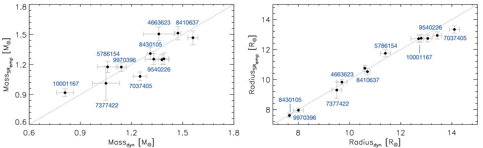
Figure 13: Asteroseismic versus dynamical masses (left) and radii (right) for nine RGB components in known eclipsing binary systems with KIC numbers indicated. Asteroseismic stellar parameters (SR_emp) were determined by using $\Delta\nu_{\rm ref,emp}\sim 131\,\mu$Hz (Section 4.2).

5 Conclusions

We find agreement between the stellar parameters determined using asteroseismic scaling relations and eclipse modelling only when using a $\Delta\nu$ reference that we derived empirically and that can be justified by known physical parameters such as mass, effective temperature, metallicity and the surface effect. In Table 10 we show the relative differences of the asteroseismic stellar parameters for the red-giant components of KIC 8410637, KIC 5640750 and KIC 9540226 with respect to the binary solutions. As we look at a small sample of stars here, we cannot investigate the global differences between the asteroseismic scaling relations and orbital parameters. Yet, we performed a careful in-depth observational analysis for each of the red giants and we found consistent results for the three systems.

Calculations of detailed stellar models of the three red giants studied here are on the way. The highly-precise and accurate Kepler data can be used to fit oscillation frequencies in a large number of red-giant stars, which provide additional information for stellar models. The oscillation frequencies, however, have to be corrected for surface effects before they can be compared to modelled frequencies (e.g. Ball & Gizon, 2017). The surface effects in red giants are not yet fully understood, even though 3-D simulations are insightful (Sonoi et al., 2015, for instance). The results from detailed modelling of the surface effects of these three red giants in eclipsing binary systems using individual frequencies is presented in Ball et al. (2018). We note however that for the red giants investigated here we require a lower $\Delta\nu$ reference value of the order of $131\,\mu$Hz when mass, temperature and metallicity dependence as well as surface effect are taken into account. This supports the idea of using $\Delta\nu_{\rm ref,emp}=130.8\pm 0.9\,\mu$Hz which in our case provides consistencies between asteroseismic and dynamical stellar parameters for KIC 8410637, KIC 5640750 and KIC 9540226 which are all located close to the red giant branch bump.

The current study shows the importance of $\Delta\nu_{\rm ref}$ in the asteroseismic scaling relations. Ideally, we would extend this work to more pulsating red-giant stars in eclipsing binary systems that cover a wide range in stellar parameters. In future, stars with different properties of mass, metallicity and evolutionary stages (e.g. red-giant components in eclipsing binaries that are in the red clump phase) need to be studied in order to identify appropriate reference values and to investigate the presence of other sources that could influence the stellar parameter measurements.

Appendix A Radial velocity measurements for KIC 8410637, KIC 5640750 and KIC 9540226

We applied the cross-correlation method to all available spectra of KIC 8410637, KIC 5640750 and KIC 9540226 to determine the radial velocities of the giants and their corresponding uncertainties, which are given in Tables 11, 12 and 13. For completeness, we also report the RVs for the dwarf components of these systems, which were obtained by previous studies.

Table 11: Radial velocity measurements of the two components of KIC 8410637. These are the measurements used in the analysis in Section 2.3. They were not used in the determination of the physical properties of the system (which was done with the velocity amplitudes from the spectral disentangling analysis). The RVs in this table are those used by co-author JS in his analysis in Section 2.3 and also in Frandsen et al. (2013). However, it was retrospectively discovered that they are not the same as those published in Frandsen et al. (2013), and source of the discrepancy has resisted our attempts to find it (S. Frandsen, 2015, priv. comm.). In future we advise that analyses of this binary system use the results from spectral disentangling, or as a second choice the RVs published in Frandsen et al. (2013). We report the RVs in this table only for completeness.

KIC 8410637
HJD-2450000	Giant RV [ km s-1]		Dwarf RV [ km s-1]		Source
5660.7131	-54.69	$\pm$ 0.05	-30.68	$\pm$ 2.59	Fies
5660.7362	-54.69	$\pm$ 0.04	-30.23	$\pm$ 2.31	Fies
5733.6205	-60.91	$\pm$ 0.05	-27.79	$\pm$ 0.76	Fies
5749.5119	-62.18	$\pm$ 0.05	-27.39	$\pm$ 0.74	Fies
5762.6434	-62.98	$\pm$ 0.06	-26.92	$\pm$ 0.88	Fies
5795.4991	-56.90	$\pm$ 0.05	-29.78	$\pm$ 1.04	Fies
5810.4756	-28.70	$\pm$ 0.05	-64.60	$\pm$ 1.38	Fies
5825.3478	-11.75	$\pm$ 0.05	-85.47	$\pm$ 1.21	Fies
5828.3417	-12.90	$\pm$ 0.05	-84.60	$\pm$ 1.30	Fies
5834.4285	-16.01	$\pm$ 0.06	-81.75	$\pm$ 1.21	Fies
5844.3966	-21.13	$\pm$ 0.05	-76.04	$\pm$ 1.79	Fies
5855.3398	-25.64	$\pm$ 0.05	-68.46	$\pm$ 1.59	Fies
5886.3003	-34.33	$\pm$ 0.05	-58.98	$\pm$ 1.15	Fies
5903.3175	-37.68	$\pm$ 0.06	-58.22	$\pm$ 1.18	Fies
5903.3444	-37.80	$\pm$ 0.07	-57.31	$\pm$ 1.55	Fies
5700.4998	-58.00	$\pm$ 0.05	-29.28	$\pm$ 1.14	Ces
5726.4642	-60.47	$\pm$ 0.06	-28.01	$\pm$ 1.27	Ces
5734.4230	-60.87	$\pm$ 0.06	-26.41	$\pm$ 2.28	Ces
5734.5069	-60.84	$\pm$ 0.07	-27.56	$\pm$ 1.29	Ces
5754.4370	-62.55	$\pm$ 0.06	-26.19	$\pm$ 1.19	Ces
5793.3535	-58.62	$\pm$ 0.05	-29.30	$\pm$ 1.48	Ces
5799.4801	-53.04	$\pm$ 0.10	-30.89	$\pm$ 1.52	Ces
5810.4495	-28.76	$\pm$ 0.06	-66.44	$\pm$ 2.19	Ces
5817.3353	-14.40	$\pm$ 0.08	-83.10	$\pm$ 1.85	Ces
5850.3024	-23.98	$\pm$ 0.06	-76.39	$\pm$ 2.48	Ces
5852.2713	-24.85	$\pm$ 0.06	-76.17	$\pm$ 3.31	Ces
5880.2040	-33.14	$\pm$ 0.05	-59.91	$\pm$ 1.48	Ces
5334.5342	-61.94	$\pm$ 0.04	-27.85	$\pm$ 0.82	Hermes
5334.6737	-61.53	$\pm$ 0.05	-27.59	$\pm$ 0.84	Hermes
5335.5792	-61.90	$\pm$ 0.04	-27.90	$\pm$ 0.74	Hermes
5335.6967	-61.58	$\pm$ 0.05	-27.48	$\pm$ 0.88	Hermes
5336.5676	-61.88	$\pm$ 0.05	-27.69	$\pm$ 0.78	Hermes
5336.7291	-61.47	$\pm$ 0.05	-27.26	$\pm$ 1.04	Hermes
5609.7553	-50.64	$\pm$ 0.04	-30.81	$\pm$ 1.69	Hermes
5715.4610	-59.72	$\pm$ 0.05	-28.80	$\pm$ 1.68	Hermes
5765.4437	-63.07	$\pm$ 0.05	-26.82	$\pm$ 0.98	Hermes
5779.4483	-63.58	$\pm$ 0.04	-27.28	$\pm$ 0.88	Hermes
5801.4416	-49.85	$\pm$ 0.05	-41.61	$\pm$ 2.13	Hermes
5835.3802	-16.82	$\pm$ 0.05	-82.05	$\pm$ 1.41	Hermes
5871.3083	-30.75	$\pm$ 0.05	-62.92	$\pm$ 1.61	Hermes
5888.3093	-35.35	$\pm$ 0.05	-58.77	$\pm$ 1.00	Hermes
5888.3273	-34.80	$\pm$ 0.05	-59.05	$\pm$ 1.21	Hermes
5965.7723	-45.72	$\pm$ 0.05	-34.82	$\pm$ 1.41	Hermes

Table 12: Radial velocity measurements of the red-giant component of KIC 5640750 derived with the cross-correlation method (ccf) from Hermes spectra.

KIC 5640750
HJD-2450000	Giant RV [ km s-1]		S/N (Mg i triplet)	Source
5623.7602	-23.34	$\pm$ 0.04	41.80	Hermes
5765.5211	-27.56	$\pm$ 0.03	32.00	Hermes
5778.6673	-28.13	$\pm$ 0.03	31.10	Hermes
5835.4160	-30.93	$\pm$ 0.03	32.00	Hermes
5867.3840	-32.67	$\pm$ 0.03	26.20	Hermes
5870.3324	-32.83	$\pm$ 0.03	27.10	Hermes
6011.7324	-43.42	$\pm$ 0.04	29.30	Hermes
6101.5477	-50.77	$\pm$ 0.03	37.00	Hermes
6101.5691	-50.76	$\pm$ 0.03	38.10	Hermes
6119.4962	-51.43	$\pm$ 0.04	36.80	Hermes
6119.5199	-51.43	$\pm$ 0.04	37.50	Hermes
6138.4671	-51.53	$\pm$ 0.03	25.70	Hermes
6138.4908	-51.53	$\pm$ 0.04	24.90	Hermes
6176.4195	-49.03	$\pm$ 0.03	33.90	Hermes
6182.4333	-48.36	$\pm$ 0.03	35.70	Hermes
6183.4953	-48.24	$\pm$ 0.03	38.70	Hermes
6183.5190	-48.22	$\pm$ 0.04	37.50	Hermes
6196.5769	-46.42	$\pm$ 0.03	26.80	Hermes
6215.3964	-43.59	$\pm$ 0.04	38.30	Hermes
6479.6168	-22.34	$\pm$ 0.03	20.10	Hermes
6484.4643	-22.42	$\pm$ 0.04	20.80	Hermes
6488.5134	-22.32	$\pm$ 0.04	20.30	Hermes

Table 13: Radial velocity measurements of the red-giant component of KIC 9540226 derived with ccf from Hermes spectra.

KIC 9540226
HJD-2450000	Giant RV [ km s-1]		S/N (Mg i triplet)	Source
5765.4977	-25.85	$\pm$ 0.03	29.60	Hermes
5783.5060	-22.50	$\pm$ 0.03	32.80	Hermes
5872.3865	-12.13	$\pm$ 0.04	27.10	Hermes
5884.3425	-19.18	$\pm$ 0.04	21.80	Hermes
5884.3570	-19.19	$\pm$ 0.05	19.90	Hermes
5889.3317	-21.16	$\pm$ 0.05	16.70	Hermes
5889.3459	-21.30	$\pm$ 0.04	10.90	Hermes
5889.3662	-21.18	$\pm$ 0.04	18.40	Hermes
5990.7423	-5.01	$\pm$ 0.04	22.90	Hermes
6106.4950	-26.43	$\pm$ 0.03	25.40	Hermes
6106.5165	-26.41	$\pm$ 0.04	26.90	Hermes
6126.6582	-24.17	$\pm$ 0.04	24.40	Hermes
6126.6796	-24.22	$\pm$ 0.03	24.10	Hermes
6132.5252	-22.91	$\pm$ 0.04	27.60	Hermes
6132.5471	-22.84	$\pm$ 0.04	25.60	Hermes
6136.6113	-21.65	$\pm$ 0.03	32.20	Hermes
6136.6327	-21.61	$\pm$ 0.03	31.70	Hermes
6139.4500	-21.00	$\pm$ 0.04	31.50	Hermes
6148.5050	-17.38	$\pm$ 0.04	32.10	Hermes
6148.5264	-17.36	$\pm$ 0.04	32.10	Hermes
6158.4969	-11.59	$\pm$ 0.04	34.20	Hermes
6158.5183	-11.58	$\pm$ 0.04	35.00	Hermes
6176.4456	6.03	$\pm$ 0.04	30.10	Hermes
6182.4104	13.44	$\pm$ 0.04	33.40	Hermes
6184.5669	15.87	$\pm$ 0.03	31.40	Hermes
6184.5895	15.92	$\pm$ 0.03	29.50	Hermes
6195.5294	18.81	$\pm$ 0.04	30.60	Hermes
6506.4110	-13.52	$\pm$ 0.03	21.90	Hermes
6506.4324	-13.55	$\pm$ 0.04	20.70	Hermes
6510.5030	-10.81	$\pm$ 0.03	16.50	Hermes
6518.3925	-4.06	$\pm$ 0.04	26.10	Hermes
6519.4668	-2.94	$\pm$ 0.04	26.70	Hermes

Appendix B Frequencies

B.1 Peakbagging results

Based on the methods described in Section 3.3.2, we extracted all the significant frequencies from the oscillation spectra of the three stars. The complete list of central mode frequencies, amplitudes and linewidths are reported in Tables 14, 15 and 16. In addition, we show the linewidths of all significant $\ell=0$ and $\ell=2$ modes in Figure 14. It is clear that the extracted non-radial modes incorporate contributions from unresolved mixed and rotationally-split modes. For KIC 8410637, KIC 5640750 and KIC 9540226 we derived linewidths of the same order of magnitude as reported by Corsaro et al. (2015b). They performed an extensive peakbagging analysis of 19 red-giant stars and they pointed out a linewidth depression close to the frequency of maximum oscillation power which is also visible in Figure 14.

Table 14: Median values and 68 per cent confidence interval for central mode frequencies, mode amplitudes and mode heights for KIC 8410637.

KIC 8410637
$n$	$\ell$	$\nu$ [$\mu$Hz]	A [ppm]	$\Gamma$ [$\mu$Hz]
5	2	32.13$\pm$0.05	47.6$\pm$6.3	0.43$\pm$0.11
6	0	32.79$\pm$0.02	40.6$\pm$3.6	0.08$\pm$0.03
6	1	35.16$\pm$0.04	52.1$\pm$4.9	0.45$\pm$0.11
6	2	36.56$\pm$0.03	66.7$\pm$7.1	0.38$\pm$0.09
7	0	37.18$\pm$0.02	46.1$\pm$5.4	0.14$\pm$0.05
6	3	37.70$\pm$0.09	12.3$\pm$6.4	0.33$\pm$0.13
7	1	39.44$\pm$0.02	87.4$\pm$6.8	0.23$\pm$0.04
7	2	41.02$\pm$0.01	62.5$\pm$6.2	0.10$\pm$0.03
8	0	41.62$\pm$0.01	88.0$\pm$5.6	0.09$\pm$0.02
8	1	44.06$\pm$0.02	90.4$\pm$6.3	0.26$\pm$0.04
8	2	45.69$\pm$0.01	87.4$\pm$5.0	0.14$\pm$0.03
9	0	46.28$\pm$0.02	94.5$\pm$6.3	0.13$\pm$0.03
8	3	47.19$\pm$0.01	29.6$\pm$4.2	0.07$\pm$0.03
9	1	48.70$\pm$0.02	93.3$\pm$5.7	0.21$\pm$0.03
9	2	50.31$\pm$0.02	96.4$\pm$7.1	0.14$\pm$0.03
10	0	50.85$\pm$0.01	87.3$\pm$5.0	0.11$\pm$0.03
9	3	51.71$\pm$0.06	37.2$\pm$5.1	0.48$\pm$0.13
10	1	53.32$\pm$0.02	81.4$\pm$4.0	0.30$\pm$0.04
10	2	55.06$\pm$0.04	75.1$\pm$8.6	0.48$\pm$0.11
11	0	55.54$\pm$0.03	61.4$\pm$7.7	0.24$\pm$0.05
11	1	58.04$\pm$0.04	64.5$\pm$3.7	0.46$\pm$0.04
11	2	59.74$\pm$0.05	47.6$\pm$8.4	0.44$\pm$0.16
12	0	60.28$\pm$0.05	62.0$\pm$7.0	0.44$\pm$0.05
12	1	62.95$\pm$0.02	82.7$\pm$4.6	0.50$\pm$0.01

Table 15: Same as Table 14 for KIC 5640750.

KIC 5640750
$n$	$\ell$	$\nu$ [$\mu$Hz]	A [ppm]	$\Gamma$ [$\mu$Hz]
3	2	14.47$\pm$0.06	18.9$\pm$17.0	0.09$\pm$0.05
4	0	14.86$\pm$0.06	48.1$\pm$19.1	0.08$\pm$0.05
4	1	16.46$\pm$0.03	86.2$\pm$11.9	0.10$\pm$0.06
4	2	17.29$\pm$0.03	53.5$\pm$11.8	0.12$\pm$0.08
5	0	17.76$\pm$0.02	75.1$\pm$12.7	0.09$\pm$0.04
5	1	19.27$\pm$0.01	142.2$\pm$14.9	0.06$\pm$0.03
5	2	20.09$\pm$0.01	107.6$\pm$11.1	0.14$\pm$0.04
6	0	20.52$\pm$0.02	99.8$\pm$08.4	0.16$\pm$0.04
5	3	20.94$\pm$0.07	51.8$\pm$14.6	0.06$\pm$0.02
6	1	22.12$\pm$0.01	140.6$\pm$12.0	0.12$\pm$0.03
6	2	23.09$\pm$0.01	141.1$\pm$15.7	0.04$\pm$0.01
7	0	23.52$\pm$0.01	187.4$\pm$16.1	0.04$\pm$0.01
6	3	24.02$\pm$0.02	57.4$\pm$10.7	0.13$\pm$0.06
7	1	25.09$\pm$0.01	182.4$\pm$11.7	0.15$\pm$0.02
7	2	26.06$\pm$0.02	178.5$\pm$12.1	0.15$\pm$0.04
8	0	26.47$\pm$0.02	128.8$\pm$13.2	0.09$\pm$0.04
8	1	28.02$\pm$0.02	147.2$\pm$10.3	0.19$\pm$0.03
8	2	29.07$\pm$0.03	127.2$\pm$24.2	0.33$\pm$0.14
9	0	29.43$\pm$0.08	99.9$\pm$23.3	0.47$\pm$0.09
9	1	31.08$\pm$0.04	93.1$\pm$07.1	0.38$\pm$0.09
9	2	32.21$\pm$0.05	70.0$\pm$13.4	0.46$\pm$0.11
10	0	32.72$\pm$0.06	66.9$\pm$12.8	0.48$\pm$0.12
10	1	34.23$\pm$0.06	58.4$\pm$06.7	0.42$\pm$0.07
10	2	35.36$\pm$0.08	60.3$\pm$06.2	0.43$\pm$0.05
11	0	35.99$\pm$0.05	64.4$\pm$11.5	0.49$\pm$0.03

Table 16: Same as Table 14 for KIC 9540226.

KIC 9540226
$n$	$\ell$	$\nu$ [$\mu$Hz]	A [ppm]	$\Gamma$ [$\mu$Hz]
5	0	19.24$\pm$0.02	66.1$\pm$10.2	0.06$\pm$0.03
5	1	20.90$\pm$0.04	140.8$\pm$09.0	0.47$\pm$0.09
5	2	21.88$\pm$0.04	38.3$\pm$10.1	0.12$\pm$0.09
6	0	22.27$\pm$0.02	97.3$\pm$09.5	0.20$\pm$0.04
6	1	23.84$\pm$0.02	130.6$\pm$09.1	0.23$\pm$0.06
6	2	24.83$\pm$0.03	129.7$\pm$08.7	0.37$\pm$0.09
7	0	25.36$\pm$0.01	99.8$\pm$11.8	0.06$\pm$0.02
7	1	27.09$\pm$0.01	172.0$\pm$12.2	0.11$\pm$0.03
7	2	28.19$\pm$0.02	135.6$\pm$12.6	0.12$\pm$0.05
8	0	28.58$\pm$0.01	144.1$\pm$13.0	0.13$\pm$0.04
8	1	30.24$\pm$0.01	154.8$\pm$10.9	0.17$\pm$0.03
8	2	31.32$\pm$0.04	97.2$\pm$14.8	0.22$\pm$0.10
9	0	31.71$\pm$0.02	127.2$\pm$13.2	0.21$\pm$0.04
9	1	33.46$\pm$0.03	111.7$\pm$05.9	0.48$\pm$0.06
9	2	34.69$\pm$0.05	53.4$\pm$09.7	0.41$\pm$0.08
10	0	35.21$\pm$0.04	83.5$\pm$10.3	0.45$\pm$0.04

Figure 14: Mode linewidths of significant frequencies of KIC 8410637 (left), KIC 5640750 (middle) and KIC 9540226 (right). Red circles and blue squares represent $\ell=0$ and $\ell=2$ modes, respectively.

B.2 Échelle diagrams

Échelle diagrams (Grec et al., 1983) present an alternative technique to identify modes of different spherical degree $\ell$. To construct such a diagram the Fourier power density spectrum is divided into segments of equal lengths ($\Delta\nu$). Then these segments are stacked on top of each other. The modes of the same spherical degree line up as near vertical ridges in the diagram. Figure 15 shows the échelle diagrams for KIC 8410637, KIC 5640750 and KIC 9540226. Three ridges are clearly visible, which correspond to spherical degrees $\ell=0,1,2$. The strongest mode frequencies that were extracted through the peakbagging analysis are marked with symbols.

Figure 15: Échelle diagrams for KIC 8410637 (left), KIC 5640750 (middle) and KIC 9540226 (right). Darker blue tones correspond to higher power. Extracted mode frequencies are indicated by symbols (square: $\ell=0$, triangle: $\ell=2$, diamond: $\ell=1$, plus: $\ell=3$) and the horizontal dotted lines show measured $\nu_{\rm max}$ values.

B.3 Differences between asteroseismic methods

The global oscillation parameters and frequencies of oscillation modes were derived independently from several co-authors using different approaches. We refer the interested reader to Mosser & Appourchaux (2009) (EACF, hereafter M09), Kallinger et al. (2014) (hereafter K14) and Corsaro & De Ridder (2014); Corsaro et al. (2015b) (Diamonds, hereafter C14), for detailed descriptions of these methods. Figure 16 shows that the seismic parameter estimates, $\nu_{\rm max}$ and $\Delta\nu$, are of the same order of magnitude and that the use of different procedures does not substantially affect the results. Based on our analysis (Section 3.3.3) we determined a local ($\Delta\nu_{\rm c}$) and global ($\Delta\nu$) mean large frequency separation, which are shown in the same Figure.

Figure 16: Estimates of the global oscillation parameters from different methods for KIC 8410637 (left), KIC 5640750 (middle) and KIC 9540226 (right). The red and gold star symbols represent the global ($\Delta\nu$) and local ($\Delta\nu_{\rm c}$) mean large frequency separations that were used to determine the stellar parameters and evolutionary stages of the red giants. The KIC number is indicated in each panel.

B.4 Second frequency differences and acoustic glitches

In addition to the first frequency difference i.e. the large frequency separation $\Delta\nu_{\rm n,\ell}$ which is given by:

$$\Delta\nu_{\rm n,\ell}\equiv\nu_{\rm n+1,\ell}-\nu_{\rm n,\ell},$$ (7)

we also computed the second frequency difference $\Delta_{\rm 2}\nu_{\rm n,\ell}$ (Gough, 1990):

$$\Delta_{\rm 2}\nu_{\rm n,\ell}\equiv\Delta\nu_{\rm n,\ell}-\Delta\nu_{\rm n-1,\ell}=\nu_{\rm n-1,\ell}-2\nu_{\rm n,\ell}+\nu_{\rm n+1,\ell}.$$ (8)

In both Equations (7–8) $\nu_{\rm n,\ell}$ represents the frequency of a mode with given radial order $n$ and spherical degree $\ell$. The first and second frequency differences of the radial ($\ell=0$) modes for KIC 8410637, KIC 5640750 and KIC 9540226 are shown in Figure 17. The uncertainties in $\Delta\nu_{\rm n,\ell}$ and $\Delta_{2}\nu_{\rm n,\ell}$ were derived from a standard error propagation of the uncertainties of the individual mode frequencies. The oscillatory signal which is visible in the second frequency difference is caused by a so-called acoustic glitch. This observable feature appears due to changes in the stellar interior that occur at scales shorter than the local wavelengths of the oscillations. In red giants, such a change is caused by the helium second ionization zone. Recently, acoustic glitch signatures could be examined in modelled and observed oscillation frequencies of stars exhibiting solar-like oscillations (e.g. Miglio et al., 2010; Mazumdar et al., 2014; Broomhall et al., 2014; Corsaro et al., 2015a; Vrard et al., 2015; Pérez Hernández et al., 2016).

Figure 17: First (top panels, Eq. 7) and second (bottom panels, Eq. 8) frequency differences for KIC 8410637, KIC 5640750 and KIC 9540226. The red solid lines indicate the fits of the acoustic glitches (Eq. 9 and Table 17) to the second differences. Uncertainties are shown on all points. In some cases the error bars are smaller than the symbol size.

In the current analysis we show that it is possible to perform a basic study of the acoustic glitches of two of the red giants (KIC 8410637 and KIC 5640750) for which we have 4 years of nearly uninterrupted Kepler data without any larger gaps available. Since this periodic signature caused by the helium second ionization zone is observable in pure p modes (e.g. Vorontsov, 1988; Gough, 1990), we can measure the acoustic depth and width of the helium second ionization zone (Hekker et al., 2013a) through the analysis of the second frequency differences of $\ell=0$ modes. The modulation due to the glitch can be described by the following model (Houdek & Gough, 2007):

$$\Delta_{\rm 2}\omega_{\rm n,\ell}=A_{\rm osc}\omega_{\rm n,\ell}\exp{(-2b_{\rm osc}^{2}\omega^{2}_{\rm n,\ell})}\cos{[2(\tau_{\rm HeII}\omega_{\rm n,\ell}+\phi)]}+c,$$ (9)

where $\omega_{\rm n,\ell}$ and $\Delta_{2}\omega_{\rm n,\ell}$ define the angular versions of $\nu_{\rm n,\ell}$ and $\Delta_{2}\nu_{\rm n,\ell}$:

$$\omega_{\rm n,\ell}\equiv 2\pi\nu_{\rm n,\ell},\\ \Delta_{\rm 2}\omega_{\rm n,\ell}\equiv 2\pi\Delta_{2}\nu_{\rm n,\ell}.$$ (10)

This model is composed of a dimensionless amplitude $A_{\rm osc}$, an acoustic depth $\tau_{\rm HeII}$ and characteristic width $b_{\rm osc}$ of the second ionization zone, a constant phase shift $\phi$ and an offset $c$. Based on the Bayesian MCMC method with Metropolis-Hastings sampling which is described in more detail in Section 3.2, we estimated the model parameters in Equation 9 and their 68 per cent credible intervals. In this case we assumed that the parameters follow a Gaussian distribution and therefore used a normal likelihood function. We did not account for correlations between the individual second frequency differences. For the free parameters, we chose uniform priors and a strict constraint on the period $\tau_{\rm HeII}$ with the convention that at least two measurements of the second frequency differences should cover one period of the acoustic glitch. The bottom panels in Figure 17 show a fit of the acoustic glitch model to the second frequency differences of KIC 8410637 and KIC 5640750 and are based on the best-fit parameters presented in Table 17. Due to a low number of available second frequency differences (less than five) we omitted KIC 9540226 (Fig. 17) from this part of the analysis.

Table 17: Median values and corresponding 68 per cent credible interval as derived for the fit parameters of the glitch model (Eq. 9) using the Metropolis-Hastings MCMC algorithm.

KIC	$A_{\rm osc}$	$\tau_{\rm HeII}$ [s]	$b_{\rm osc}$ [s]	$\phi$ [rad]	$c$ [$\mu$Hz]
8410637	$0.041\pm 0.003$	$40437\pm 16$	$3875\pm 23$	$2.33\pm 0.01$	$0.06\pm 0.01$
5640750	$0.020\pm 0.007$	$62901\pm 4281$	$4118\pm 656$	$1.08\pm 0.67$	$0.09\pm 0.04$

References

- Anderson et al. (1990) Anderson E. R., Duvall Jr. T. L., Jefferies S. M., 1990, ApJ, 364, 699
- Appourchaux (2003) Appourchaux T., 2003, A&A, 412, 903
- Baglin et al. (2007) Baglin A., Auvergne M., Barge P., Michel E., Catala C., Deleuil M., Weiss W., 2007, in Dumitrache C., Popescu N. A., Suran M. D., Mioc V., eds, American Institute of Physics Conference Series Vol. 895, Fifty Years of Romanian Astrophysics. pp 201–209, doi:10.1063/1.2720423
- Ball & Gizon (2017) Ball W. H., Gizon L., 2017, A&A, 600, A128
- Ball et al. (2018) Ball W. H., Themeßl N., Hekker S., 2018, MNRAS
- Barban et al. (2007) Barban C., et al., 2007, A&A, 468, 1033
- Basu et al. (2010) Basu S., Chaplin W. J., Elsworth Y., 2010, ApJ, 710, 1596
- Beck et al. (2011) Beck P. G., et al., 2011, Science, 332, 205
- Beck et al. (2012) Beck P. G., et al., 2012, Nature, 481, 55
- Beck et al. (2014) Beck P. G., et al., 2014, A&A, 564, A36
- Bedding et al. (2011) Bedding T. R., et al., 2011, Nature, 471, 608
- Belkacem et al. (2011) Belkacem K., Goupil M. J., Dupret M. A., Samadi R., Baudin F., Noels A., Mosser B., 2011, A&A, 530, A142
- Belkacem et al. (2013) Belkacem K., Samadi R., Mosser B., Goupil M.-J., Ludwig H.-G., 2013, in Shibahashi H., Lynas-Gray A. E., eds, Astronomical Society of the Pacific Conference Series Vol. 479, Progress in Physics of the Sun and Stars: A New Era in Helio- and Asteroseismology. p. 61 (arXiv:1307.3132)
- Borucki et al. (2010) Borucki W. J., et al., 2010, Science, 327, 977
- Brogaard et al. (2016) Brogaard K., et al., 2016, preprint, (arXiv:1601.01412)
- Brogaard et al. (2018) Brogaard K., et al., 2018, preprint, (arXiv:1801.08167)
- Broomhall et al. (2014) Broomhall A.-M., et al., 2014, MNRAS, 440, 1828
- Brown et al. (1991) Brown T. M., Gilliland R. L., Noyes R. W., Ramsey L. W., 1991, ApJ, 368, 599
- Brown et al. (2011) Brown T. M., Latham D. W., Everett M. E., Esquerdo G. A., 2011, AJ, 142, 112
- Bruntt et al. (2004) Bruntt H., et al., 2004, A&A, 425, 683
- Carter et al. (2008) Carter J. A., Yee J. C., Eastman J., Gaudi B. S., Winn J. N., 2008, ApJ, 689, 499
- Casagrande et al. (2016) Casagrande L., et al., 2016, MNRAS, 455, 987
- Cassisi & Salaris (1997) Cassisi S., Salaris M., 1997, MNRAS, 285, 593
- Christensen-Dalsgaard et al. (2014) Christensen-Dalsgaard J., Silva Aguirre V., Elsworth Y., Hekker S., 2014, MNRAS, 445, 3685
- Corsaro & De Ridder (2014) Corsaro E., De Ridder J., 2014, A&A, 571, A71
- Corsaro et al. (2012) Corsaro E., et al., 2012, ApJ, 757, 190
- Corsaro et al. (2015a) Corsaro E., De Ridder J., García R. A., 2015a, A&A, 578, A76
- Corsaro et al. (2015b) Corsaro E., De Ridder J., García R. A., 2015b, A&A, 579, A83
- Davies et al. (2016) Davies G. R., et al., 2016, MNRAS, 456, 2183
- De Ridder et al. (2009) De Ridder J., et al., 2009, Nature, 459, 398
- Duvall & Harvey (1986) Duvall Jr. T. L., Harvey J. W., 1986, in Gough D. O., ed., NATO Advanced Science Institutes (ASI) Series C Vol. 169, NATO Advanced Science Institutes (ASI) Series C. pp 105–116
- Elsworth et al. (2017) Elsworth Y., Hekker S., Basu S., Davies G. R., 2017, MNRAS, 466, 3344
- Frandsen et al. (2013) Frandsen S., et al., 2013, A&A, 556, A138
- Fröhlich et al. (1995) Fröhlich C., et al., 1995, Sol. Phys., 162, 101
- Gai et al. (2011) Gai N., Basu S., Chaplin W. J., Elsworth Y., 2011, ApJ, 730, 63
- Gaia Collaboration et al. (2016) Gaia Collaboration et al., 2016, A&A, 595, A2
- Gaulme et al. (2013) Gaulme P., McKeever J., Rawls M. L., Jackiewicz J., Mosser B., Guzik J. A., 2013, ApJ, 767, 82
- Gaulme et al. (2014) Gaulme P., Jackiewicz J., Appourchaux T., Mosser B., 2014, ApJ, 785, 5
- Gaulme et al. (2016) Gaulme P., et al., 2016, ApJ, 832, 121
- Girardi et al. (2002) Girardi L., Bertelli G., Bressan A., Chiosi C., Groenewegen M. A. T., Marigo P., Salasnich B., Weiss A., 2002, A&A, 391, 195
- Gough (1990) Gough D. O., 1990, in Osaki Y., Shibahashi H., eds, Lecture Notes in Physics, Berlin Springer Verlag Vol. 367, Progress of Seismology of the Sun and Stars. p. 283, doi:10.1007/3-540-53091-6
- Grec et al. (1983) Grec G., Fossat E., Pomerantz M. A., 1983, Sol. Phys., 82, 55
- Guggenberger et al. (2016) Guggenberger E., Hekker S., Basu S., Bellinger E., 2016, MNRAS,
- Guggenberger et al. (2017) Guggenberger E., Hekker S., Angelou G. C., Basu S., Bellinger E. P., 2017, MNRAS, 470, 2069
- Hadrava (1995) Hadrava P., 1995, A&AS, 114, 393
- Handberg & Campante (2011) Handberg R., Campante T. L., 2011, A&A, 527, A56
- Handberg & Lund (2014) Handberg R., Lund M. N., 2014, MNRAS, 445, 2698
- Handberg et al. (2017) Handberg R., Brogaard K., Miglio A., Bossini D., Elsworth Y., Slumstrup D., Davies G. R., Chaplin W. J., 2017, MNRAS, 472, 979
- Hekker (2013) Hekker S., 2013, Advances in Space Research, 52, 1581
- Hekker & Christensen-Dalsgaard (2017) Hekker S., Christensen-Dalsgaard J., 2017, A&ARv, 25
- Hekker et al. (2009) Hekker S., et al., 2009, A&A, 506, 465
- Hekker et al. (2010) Hekker S., et al., 2010, ApJ, 713, L187
- Hekker et al. (2011a) Hekker S., et al., 2011a, A&A, 525, A131
- Hekker et al. (2011b) Hekker S., et al., 2011b, A&A, 530, A100
- Hekker et al. (2012) Hekker S., et al., 2012, A&A, 544, A90
- Hekker et al. (2013a) Hekker S., Basu S., Elsworth Y., Chaplin W. J., 2013a, in Suárez J. C., Garrido R., Balona L. A., Christensen-Dalsgaard J., eds, Astrophysics and Space Science Proceedings Vol. 31, Stellar Pulsations: Impact of New Instrumentation and New Insights. p. 73 (arXiv:1203.4588), doi:10.1007/978-3-642-29630-7_14
- Hekker et al. (2013b) Hekker S., Elsworth Y., Mosser B., Kallinger T., Basu S., Chaplin W. J., Stello D., 2013b, A&A, 556, A59
- Henden et al. (2012) Henden A. A., Levine S. E., Terrell D., Smith T. C., Welch D., 2012, Journal of the American Association of Variable Star Observers (JAAVSO), 40, 430
- Hensberge & Pavlovski (2007) Hensberge H., Pavlovski K., 2007, in Hartkopf W. I., Harmanec P., Guinan E. F., eds, IAU Symposium Vol. 240, Binary Stars as Critical Tools & Tests in Contemporary Astrophysics. pp 136–147 (arXiv:astro-ph/0611422), doi:10.1017/S1743921307003948
- Hensberge et al. (2008) Hensberge H., Ilijić S., Torres K. B. V., 2008, A&A, 482, 1031
- Hilditch (2001) Hilditch R. W., 2001, An Introduction to Close Binary Stars
- Houdek & Gough (2007) Houdek G., Gough D. O., 2007, MNRAS, 375, 861
- Huber (2014) Huber D., 2014, preprint (arXiv:1404.7501)
- Huber et al. (2010) Huber D., et al., 2010, ApJ, 723, 1607
- Huber et al. (2014) Huber D., et al., 2014, ApJS, 211, 2
- Ilijic et al. (2004) Ilijic S., Hensberge H., Pavlovski K., Freyhammer L. M., 2004, in Hilditch R. W., Hensberge H., Pavlovski K., eds, Astronomical Society of the Pacific Conference Series Vol. 318, Spectroscopically and Spatially Resolving the Components of the Close Binary Stars. pp 111–113
- Jiménez et al. (2002) Jiménez A., Roca Cortés T., Jiménez-Reyes S. J., 2002, Sol. Phys., 209, 247
- Kallinger et al. (2008) Kallinger T., et al., 2008, A&A, 478, 497
- Kallinger et al. (2010) Kallinger T., et al., 2010, A&A, 522, A1
- Kallinger et al. (2012) Kallinger T., et al., 2012, A&A, 541, A51
- Kallinger et al. (2014) Kallinger T., et al., 2014, A&A, 570, A41
- Kallinger et al. (2018) Kallinger T., Beck P. G., Stello D., García R. A., 2018, A&A(submitted)
- Kjeldsen & Bedding (1995) Kjeldsen H., Bedding T. R., 1995, A&A, 293
- Kolbas et al. (2015) Kolbas V., et al., 2015, MNRAS, 451, 4150
- Kopal (1950) Kopal Z., 1950, Harvard College Observatory Circular, 454, 1
- Kumar et al. (1995) Kumar P., Ao C. O., Quataert E. J., 1995, ApJ, 449, 294
- Kupka et al. (2000) Kupka F. G., Ryabchikova T. A., Piskunov N. E., Stempels H. C., Weiss W. W., 2000, Baltic Astronomy, 9, 590
- Kurucz (1993) Kurucz R., 1993, ATLAS9 Stellar Atmosphere Programs and 2 km/s grid. Kurucz CD-ROM No. 13. Cambridge, Mass.: Smithsonian Astrophysical Observatory, 1993., 13
- Libbrecht & Woodard (1990) Libbrecht K. G., Woodard M. F., 1990, Nature, 345, 779
- Mamajek et al. (2015) Mamajek E. E., et al., 2015, preprint (arXiv:1510.07674)
- Mayer et al. (2013) Mayer P., Harmanec P., Pavlovski K., 2013, A&A, 550, A2
- Mazumdar et al. (2014) Mazumdar A., et al., 2014, ApJ, 782, 18
- Miglio et al. (2010) Miglio A., et al., 2010, A&A, 520, L6
- Miglio et al. (2012) Miglio A., et al., 2012, MNRAS, 419, 2077
- Miglio et al. (2013) Miglio A., et al., 2013, MNRAS, 429, 423
- Mosser & Appourchaux (2009) Mosser B., Appourchaux T., 2009, A&A, 508, 877
- Mosser et al. (2010) Mosser B., et al., 2010, A&A, 517, A22
- Mosser et al. (2011) Mosser B., et al., 2011, A&A, 525, L9
- Mosser et al. (2012a) Mosser B., et al., 2012a, A&A, 540, A143
- Mosser et al. (2012b) Mosser B., et al., 2012b, A&A, 548, A10
- Mosser et al. (2013) Mosser B., et al., 2013, A&A, 550, A126
- Mosser et al. (2014) Mosser B., et al., 2014, A&A, 572, L5
- Mosser et al. (2015) Mosser B., Vrard M., Belkacem K., Deheuvels S., Goupil M. J., 2015, A&A, 584, A50
- Pavlovski & Hensberge (2005) Pavlovski K., Hensberge H., 2005, A&A, 439, 309
- Pavlovski & Hensberge (2010) Pavlovski K., Hensberge H., 2010, in Prša A., Zejda M., eds, Astronomical Society of the Pacific Conference Series Vol. 435, Binaries - Key to Comprehension of the Universe. p. 207 (arXiv:0909.3246)
- Pérez Hernández et al. (2016) Pérez Hernández F., García R. A., Corsaro E., Triana S. A., De Ridder J., 2016, A&A, 591, A99
- Pietrinferni et al. (2004) Pietrinferni A., Cassisi S., Salaris M., Castelli F., 2004, ApJ, 612, 168
- Pinsonneault et al. (2014) Pinsonneault M. H., et al., 2014, ApJS, 215, 19
- Press et al. (1989) Press W. H., Flannery B. P., Teukolsky S. A., Vetterling W. T., 1989, Numerical recipes in Pascal. The art of scientific computing
- Prša et al. (2016) Prša A., et al., 2016, AJ, 152, 41
- Raskin (2011) Raskin G., 2011, PhD thesis, Institute of Astronomy, Katholieke Universiteit Leuven, Belgium
- Raskin et al. (2011) Raskin G., et al., 2011, A&A, 526, A69
- Remus et al. (2012) Remus F., Mathis S., Zahn J.-P., 2012, A&A, 544, A132
- Rodrigues et al. (2017) Rodrigues T. S., et al., 2017, MNRAS, 467, 1433
- Rucinski (2002) Rucinski S. M., 2002, AJ, 124, 1746
- Salaris & Cassisi (1998) Salaris M., Cassisi S., 1998, MNRAS, 298, 166
- Sharma et al. (2016) Sharma S., Stello D., Bland-Hawthorn J., Huber D., Bedding T. R., 2016, ApJ, 822, 15
- Shulyak et al. (2004) Shulyak D., Tsymbal V., Ryabchikova T., Stütz C., Weiss W. W., 2004, A&A, 428, 993
- Simon & Sturm (1994) Simon K. P., Sturm E., 1994, A&A, 281, 286
- Sing (2010) Sing D. K., 2010, A&A, 510, A21
- Skrutskie et al. (2006) Skrutskie M. F., et al., 2006, AJ, 131, 1163
- Sneden et al. (2012) Sneden C., Bean J., Ivans I., Lucatello S., Sobeck J., 2012, MOOG: LTE line analysis and spectrum synthesis, Astrophysics Source Code Library (ascl:1202.009)
- Sonoi et al. (2015) Sonoi T., Samadi R., Belkacem K., Ludwig H.-G., Caffau E., Mosser B., 2015, A&A, 583, A112
- Southworth (2008) Southworth J., 2008, MNRAS, 386, 1644
- Southworth (2012) Southworth J., 2012, MNRAS, 426, 1291
- Southworth (2013) Southworth J., 2013, A&A, 557, A119
- Southworth et al. (2005) Southworth J., Maxted P. F. L., Smalley B., 2005, A&A, 429, 645
- Southworth et al. (2007) Southworth J., Bruntt H., Buzasi D. L., 2007, A&A, 467, 1215
- Stello et al. (2009) Stello D., Chaplin W. J., Basu S., Elsworth Y., Bedding T. R., 2009, MNRAS, 400, L80
- Tassoul (1980) Tassoul M., 1980, ApJS, 43, 469
- Tayar et al. (2017) Tayar J., et al., 2017, ApJ, 840, 17
- Themeßl et al. (2017) Themeßl N., Hekker S., Elsworth Y., 2017, in European Physical Journal Web of Conferences. p. 05009 (arXiv:1705.11155), doi:10.1051/epjconf/201716005009
- Thompson et al. (2012) Thompson S. E., et al., 2012, ApJ, 753, 86
- Tkachenko (2015) Tkachenko A., 2015, A&A, 581, A129
- Tkachenko et al. (2013) Tkachenko A., Van Reeth T., Tsymbal V., Aerts C., Kochukhov O., Debosscher J., 2013, A&A, 560, A37
- Tonry & Davis (1979) Tonry J., Davis M., 1979, AJ, 84, 1511
- Torres et al. (2014) Torres G., Sandberg Lacy C. H., Pavlovski K., Feiden G. A., Sabby J. A., Bruntt H., Viggo Clausen J., 2014, ApJ, 797, 31
- Tsymbal (1996) Tsymbal V., 1996, in Adelman S. J., Kupka F., Weiss W. W., eds, Astronomical Society of the Pacific Conference Series Vol. 108, M.A.S.S., Model Atmospheres and Spectrum Synthesis. p. 198
- Ulrich (1986) Ulrich R. K., 1986, ApJ, 306, L37
- Verner et al. (2011) Verner G. A., et al., 2011, MNRAS, 415, 3539
- Viani et al. (2017) Viani L. S., Basu S., Chaplin W. J., Davies G. R., Elsworth Y., 2017, ApJ, 843, 11
- Vorontsov (1988) Vorontsov S. V., 1988, in Christensen-Dalsgaard J., Frandsen S., eds, IAU Symposium Vol. 123, Advances in Helio- and Asteroseismology. p. 151
- Vrard et al. (2015) Vrard M., et al., 2015, A&A, 579, A84
- Vrard et al. (2016) Vrard M., Mosser B., Samadi R., 2016, A&A, 588, A87
- White et al. (2011) White T. R., Bedding T. R., Stello D., Christensen-Dalsgaard J., Huber D., Kjeldsen H., 2011, ApJ, 743, 161
- Zucker & Mazeh (1994) Zucker S., Mazeh T., 1994, ApJ, 420, 806