Analytic and numeric computation of edge states and conductivity of a Kane-Mele nanoribbon

Abstract

We compute analytic expressions for the edge states in a zigzag Kane-Mele nanoribbon (KMNR) by solving the eigenvalue equations in presence of intrinsic and Rashba spin-orbit couplings. Owing to the P-T symmetry of the Hamiltonian the edge states are protected by topological invariance and hence are found to be robust. We have done a systematic study for each of the above cases, for example, a pristine graphene, graphene with an intrinsic spin-orbit coupling, graphene with a Rashba spin-orbit coupling, a Kane-Mele nanoribbon and supported our results on the robustness of the edge states by analytic computation of the electronic probability amplitudes, the local density of states (LDOS), band structures and the conductance spectra.

1 Introduction

The successful fabrication of graphene [1] has generated intense research activities to study the electronic properties of this novel two dimensional (2D) electronic system. Graphene has a honeycomb lattice structure due to the $sp^{2}$ hybridization of carbon atoms and the $\pi$-electrons can hop between nearest neighbors. The valence and conduction bands of graphene touch each other at two nonequivalent Dirac points, $K$ and ${{K}^{\prime}}$, which have opposite chiralities and form a time-reversed pair. The band structure around those points has the Dirac form, ${{E}_{{\vec{k}}}}=\hbar v|\vec{k}|$ , where $v$ $(\simeq{{10}^{6}}$ ms^-1) is the Fermi velocity. The Dirac nature of the electrons [2] is responsible for many interesting properties of graphene [3], such as unconventional quantum Hall effect [1, 4, 5], half metallicity [6, 7], Klein tunneling through a barrier [8], high carrier mobility [9, 10] and many more. Owing to these features, graphene is recognized as one of the promising materials for realizing next-generation electronic devices.

The existence of edge states in a graphene sheet is one of the interesting features in condensed matter physics. The properties of the edge states are different than the bulk states and play important roles in transport. When the valence and conduction bands are separated by an energy gap, electrons can not flow through the bulk. However, this does not guarantee that the system is a simple insulator, since conduction may still be allowed via edge modes. These new type of insulators are different from trivial insulators due to their unique gapless edge states protected by the time-reversal symmetry and they are attributed the name topological insulators. Thus topological insulators (TIs) represent a new quantum state. The phenomena associated with the TIs are the well known quantum Hall effect and the quantum spin Hall effect, where it has been found that the gapless chiral or helical edge states are robust channels with quantized conductance accompanied by non-vanishing values at zero bias [11, 12, 13, 14, 15, 16, 17, 18].

Kane and Mele [13, 14] predicted that a quantum spin Hall (QSH) state can be observed in presence of next-nearest neighbour intrinsic spin-orbit coupling (SOC), which triggered an enormous study on topologically non-trivial electronic materials [15, 19, 20, 21]. Unfortunately, the QSH phase in pristine graphene is still not observed experimentally owing to its vanishingly small intrinsic spin-orbit coupling strength (typically $\sim$ 0.01-0.05 meV) [22, 23], whereas in strong SOC materials, such as CdTe/HgTe quantum wells, the QSH phase has been observed [24]. However, there are various ways to induce SOC in graphene experimentally, such as doping by adatoms [25], using the proximity to a three-dimensional topological insulator, such as Bi₂Se₃ [26, 27], by functionalization with methyl [28] etc.

Two kinds of SOC can be present in graphene, the intrinsic and the Rashba SOC. Recent observations showed that the strength of the Rashba SOC can also be enhanced up to 100 meV from Gold (Au) intercalation at the graphene-Ni interface [29]. A Rashba splitting about 225 meV in epitaxial graphene layers grown on the surface of Ni [30] and a giant Rashba SOC ($\sim$ 600 meV) from Pb intercalation at the graphene-Ir surface [31] are observed in experiments. In this work, we have studied the interplay between these two types of SOC on the band structure and the edge states [32] with a view to understand the data on charge conductances.

The electronic properties of GNRs depend on the geometry of the edges [33], and according to the edge termination type, mainly there are two kinds of GNR, namely armchair graphene nanoribbon (AGNR) and zigzag graphene nanoribbon (ZGNR). The ZGNRs are always metallic with zero band gap, while the AGNRs are metallic when the lateral width $N=3M-1$ ($M$ is an integer), else the AGNRs are semiconducting in nature [34] with a finite band gap. The presence of edges in graphene has strong implications for the low-energy spectrum of the $\pi$-electrons [33, 34, 35]. It was shown that ZGNRs possess localized edge states with energies close to the Fermi level. On the contrary, edge states are absent for AGNRs. We prefer to call these GNRs in presence of spin-orbit couplings as Kane-Mele nanoribbon (KMNR) and we shall deal with the zigzag variant, namely ZKMNR.

We organize our paper as follows. In the following section, for completeness and clarity of the system and its notations, we write the Kane-Mele model for a GNR and perform an analytical investigation of the edge states for a few choices of the intrinsic and Rashba spin-orbit coupling. The corresponding band structures are presented for a check. Subsequently, we include an elaborate discussion of the results where we have demonstrated the interplay of intrinsic and Rashba SOC on the charge conductances. We conclude with a brief summary of our results.

2 Kane-Mele Hamiltonian

To begin with a pristine graphene sheet which consists of two sublattices A and B connected to three nearest neighbors vectors in real space are given by, $\delta_{1}=\big{(}0,a\big{)}$; $\delta_{2}=\Big{(}\frac{\sqrt{3}a}{2},-\frac{a}{2}\Big{)}$ and $\delta_{3}=\Big{(}-\frac{\sqrt{3}a}{2},-\frac{a}{2}\Big{)}$, where $a\approx 1.42$ Å  is the carbon-carbon distance. In order to study the nature of the edge states and transport properties in presence of spin-orbit coupled term, we consider the following Kane-Mele (KM) [13, 14] Hamiltonian,

$$H= -t\sum\limits_{\langle ij\rangle\alpha}c_{i\alpha}^{\dagger}c_{j\alpha}+it_{2}\sum\limits_{\langle\langle ij\rangle\rangle\alpha\beta}\nu_{ij}c_{i\alpha}^{\dagger}s^{z}_{\alpha\beta}c_{j\beta}$$

$$+i\lambda_{R}\sum\limits_{\langle ij\rangle\alpha\beta}c_{i\alpha}^{\dagger}\left({\bf s}\times{\bf\hat{d}}_{ij}\right)_{z}c_{j\beta}$$ (1)

Here $c_{i\alpha}^{\dagger}$ and $c_{j\alpha}$ are creation and annihilation operators for an electron with spin $\alpha$ on site $i$. The first term describes the hopping between nearest neighbors $i$ and $j$ on a honeycomb lattice where the hopping amplitude is, $t$ $\simeq 2.7$ eV. The second term is the mirror symmetric intrinsic spin-orbit coupling (SOC) which involves spin-dependent second neighbor hopping between same sublattices with a coupling strength $t_{2}$. $\nu_{ij}$ = $+1(-1)$ if the electron makes a left (right) turn to go from site $j$ to $i$ through their common nearest neighbor. The vector d points from site $i$ to site $j$ and corresponds to the nearest neighbor vectors. $s^{z}$ is the $z$-component of Pauli spin matrix. The third term is the nearest neighbor Rashba term which arises due to the broken surface inversion symmetry with coupling strength $\lambda_{R}$. The spin orbit term $t_{2}$ breaks the $SU(2)$ symmetry down to $U(1)$ symmetry, the Rashba term $\lambda_{R}$ breaks the $U(1)$ symmetry down to $\mathbb{Z}_{2}$ [36]. Due to the small atomic number of carbon, the intrinsic SOC is usually weak [22, 37]. The Rashba coupling strength can be tuned by applying an external electric field.

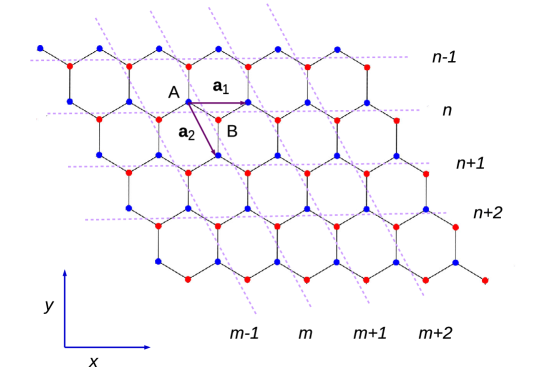
Figure 1: (Color online) Graphene nanoribbon geometry with zigzag edges. The blue and red circles represent the A and B sublattices of the ribbon. $\vec{\bf{a}}_{1}$ and $\vec{\bf{a}}_{2}$ are the primitive vectors. $(m,n)$ labels the unit cell. $m$ increases along the positive $x$-direction whereas $n$ increases along the negative $y$-direction.

3 Edge states

In this section, we study the edge state properties considering the tight-binding Hamiltonian in presence of spin-orbit and Rashba coupling. As said earlier, we focus on Kane-Mele ribbon geometry with zigzag edges which are infinite along $x$-axis and all the atoms of the zigzag edges belong to the same sublattice as shown in Fig. 1. The ribbon width is such that it has $N$ unit cells in the $y$-axis. We rewrite the equation (2), with $t_{2}$ = $\lambda_{R}$ = $0$, in terms of $m$, $n$ which labels the unit cell as shown in Fig. 1, is given by [3],

$$H= -t\sum\limits_{\langle mn\rangle\sigma}\Big{[}a^{\dagger}_{\sigma}(m,n)b_{\sigma}(m,n)+a^{\dagger}_{\sigma}(m,n)b_{\sigma}(m,n-1)$$

$$+a^{\dagger}_{\sigma}(m,n)b_{\sigma}(m-1,n)+H.C\Big{]}$$ (2)

where $\langle$ $\rangle$ denotes nearest neighbors and $\sigma$ represents the $\uparrow$,$\downarrow$ spin for both sublattices $A$ and $B$. The translational symmetry exists along $x$-axis but there is no translational symmetry along the $y$-direction due to the existence of edge state. Hence the momentum $k_{x}$ is a good quantum number. Now we can use a momentum representation of the electron operator due to the periodicity in the $x$-direction, which is,

$$c_{i}=\frac{1}{\sqrt{L_{x}}}\sum\limits_{k_{x}}\exp^{ik_{x}X_{i}}c_{k}$$ (3)

where ($X_{i}$, $Y_{i}$) represents the coordinate of the site $A$ and $B$ in the unit cell $(m,n)$ (see Fig. 1). Using Schr$\ddot{o}$dinger equation $H|\psi\rangle=E|\psi\rangle$, we get the following eigenvalue equations for sites in $A$ and $B$ sublattices as,

$$E\alpha\left(k_{x},n\right)=-t\left[2\cos\left(\frac{\sqrt{3}k_{x}}{2}\right)\beta\left(k_{x},n\right)+\beta\left(k_{x},n-1\right)\right]$$

$$E\beta\left(k_{x},n\right)=-t\left[2\cos\left(\frac{\sqrt{3}k_{x}}{2}\right)\alpha\left(k_{x},n\right)+\alpha\left(k_{x},n+1\right)\right]$$ (4)

where we have chosen the basis as,

$$|\psi_{k}\rangle=\sum\limits_{n,\sigma}\alpha(k,n,\sigma)|a,k,n,\sigma\rangle+\beta(k,n,\sigma)|b,k,n,\sigma\rangle.$$

where $\alpha$, $\beta$ are the eigenstates for the $A$ and $B$ sublattices. Since we have taken zigzag edges and the ribbon exists only between $0$ to $N-1$, and thus the boundary condition is,

$$\alpha(k_{x},n)=\beta(k_{x},-1)=0$$ (5)

and we impose $E=0$ as the plateau in the conductance is observed for $E\simeq 0$. We have made $k_{x}$ as a dimensionless quantity by absorbing the lattice spacing $a$ into the definition of $k_{x}$. We can see that the charge density is proportional to $\left[2\cos\left(\frac{\sqrt{3}k_{x}}{2}\right)\right]^{n}$ at each non-nodal site of the $n$-th zigzag chain certifying the presence of localized edge states with an exponential decay as one deviates from the edge[33]. A completely flat band exists in the special vicinity of $k_{x}$. Since the cosine term becomes zero at $k_{x}=\frac{\pi}{\sqrt{3}}$, we have taken $k_{x}=\frac{n\pi}{3\sqrt{3}}$ [38] to arrive the desired solution for a pristine graphene.

Now we consider the intrinsic spin-orbit interaction term as mentioned in Eq. (2). Using the same basis and including spin degrees of freedom we get four eigenvalue equations for spins up and down and for $A$ and $B$ sublattice points which are written as,

$$E\alpha_{\uparrow}\left(k_{x},n\right)= -t\left[2\cos\left(\frac{\sqrt{3}k_{x}}{2}\right)\beta_{\uparrow}(k_{x},n)+\beta_{\uparrow}(k_{x},n-1)\right]$$

$$-2t_{2}\Bigg{[}\sin\left(\sqrt{3}k_{x}\right)\alpha_{\uparrow}(k_{x},n)-\sin\left(\frac{\sqrt{3}k_{x}}{2}\right)\bigg{(}\alpha_{\uparrow}(k_{x},n-1)+\alpha_{\uparrow}(k_{x},n+1)\bigg{)}\Bigg{]},$$

$$E\alpha_{\downarrow}\left(k_{x},n\right)= -t\left[2\cos\left(\frac{\sqrt{3}k_{x}}{2}\right)\beta_{\downarrow}(k_{x},n)+\beta_{\downarrow}(k_{x},n-1)\right]$$

$$+2t_{2}\Bigg{[}\sin\left(\sqrt{3}k_{x}\right)\alpha_{\downarrow}(k_{x},n)-\sin\left(\frac{\sqrt{3}k_{x}}{2}\right)\bigg{(}\alpha_{\downarrow}(k_{x},n-1)+\alpha_{\downarrow}(k_{x},n+1)\bigg{)}\Bigg{]},$$

$$E\beta_{\uparrow}\left(k_{x},n\right)= -t\left[2\cos\left(\frac{\sqrt{3}k_{x}}{2}\right)\alpha_{\uparrow}(k_{x},n)+\alpha_{\uparrow}(k_{x},n+1)\right]$$

$$+2t_{2}\Bigg{[}\sin\left(\sqrt{3}k_{x}\right)\beta_{\uparrow}(k_{x},n)-\sin\left(\frac{\sqrt{3}k_{x}}{2}\right)\bigg{(}\beta_{\uparrow}(k_{x},n-1)+\beta_{\uparrow}(k_{x},n+1)\bigg{)}\Bigg{]},$$

$$E\beta_{\downarrow}\left(k_{x},n\right)= -t\left[2\cos\left(\frac{\sqrt{3}k_{x}}{2}\right)\alpha_{\downarrow}(k_{x},n)+\alpha_{\downarrow}(k_{x},n+1)\right]$$

$$-2t_{2}\Bigg{[}\sin\left(\sqrt{3}k_{x}\right)\beta_{\downarrow}(k_{x},n)-\sin\left(\frac{\sqrt{3}k_{x}}{2}\right)\bigg{(}\beta_{\downarrow}(k_{x},n-1)+\beta_{\downarrow}(k_{x},n+1)\bigg{)}\Bigg{]},$$ (6)

where $\alpha_{\uparrow,\downarrow}$ and $\beta_{\uparrow,\downarrow}$ correspond to the spin resolved eigenstates for the $A$ and $B$ sublattices. For a comprehensible solution, we turn to a numerical computation of the above set of equations. Here we have used $k_{x}=\frac{\pi}{\sqrt{3}}$ which particularly renders simple forms for the equations. Solving the above equations (Eq. 6) numerically (with $t=1$ and energy $E=0$) following the same boundary conditions (as given in Eq. 5), we shall see how the probability densities of the wavefunctions decay ascertaining whether edge states exist.

Next we turn on the other SOC, namely the Rashba spin-orbit coupling (RSOC). This yields the new set of equations for a KMNR given by [39],

$$E\alpha_{\uparrow}\left(k_{x},n\right)= - t\left[2\cos\left(\frac{\sqrt{3}k_{x}}{2}\right)\beta_{\uparrow}(k_{x},n)+\beta_{\uparrow}(k_{x},n-1)\right]$$

$$- 2t_{2}\Bigg{[}\sin\left(\sqrt{3}k_{x}\right)\alpha_{\uparrow}(k_{x},n)-\sin\left(\frac{\sqrt{3}k_{x}}{2}\right)\bigg{(}\alpha_{\uparrow}(k_{x},n-1)+\alpha_{\uparrow}(k_{x},n+1)\bigg{)}\Bigg{]}$$

$$+ i\lambda_{R}\left[\left(\cos\left(\frac{\sqrt{3}k_{x}}{2}\right)+\sqrt{3}\sin\left(\frac{\sqrt{3}k_{x}}{2}\right)\right)\beta_{\downarrow}(k_{x},n)-\beta_{\downarrow}(k_{x},n-1)\right],$$

$$E\alpha_{\downarrow}\left(k_{x},n\right)= - t\left[2\cos\left(\frac{\sqrt{3}k_{x}}{2}\right)\beta_{\downarrow}(k_{x},n)+\beta_{\downarrow}(k_{x},n-1)\right]$$

$$+ 2t_{2}\Bigg{[}\sin\left(\sqrt{3}k_{x}\right)\alpha_{\downarrow}(k_{x},n)-\sin\left(\frac{\sqrt{3}k_{x}}{2}\right)\bigg{(}\alpha_{\downarrow}(k_{x},n-1)+\alpha_{\downarrow}(k_{x},n+1)\bigg{)}\Bigg{]}$$

$$+ i\lambda_{R}\left[\left(\cos\left(\frac{\sqrt{3}k_{x}}{2}\right)-\sqrt{3}\sin\left(\frac{\sqrt{3}k_{x}}{2}\right)\right)\beta_{\uparrow}(k_{x},n)-\beta_{\uparrow}(k_{x},n-1)\right],$$

$$E\beta_{\uparrow}\left(k_{x},n\right)= - t\left[2\cos\left(\frac{\sqrt{3}k_{x}}{2}\right)\alpha_{\uparrow}(k_{x},n)+\alpha_{\uparrow}(k_{x},n+1)\right]$$

$$+ 2t_{2}\Bigg{[}\sin\left(\sqrt{3}k_{x}\right)\beta_{\uparrow}(k_{x},n)-\sin\left(\frac{\sqrt{3}k_{x}}{2}\right)\bigg{(}\beta_{\uparrow}(k_{x},n-1)+\beta_{\uparrow}(k_{x},n+1)\bigg{)}\Bigg{]}$$

$$- i\lambda_{R}\left[\left(\cos\left(\frac{\sqrt{3}k_{x}}{2}\right)-\sqrt{3}\sin\left(\frac{\sqrt{3}k_{x}}{2}\right)\right)\alpha_{\downarrow}(k_{x},n)-\alpha_{\downarrow}(k_{x},n+1)\right],$$

$$E\beta_{\downarrow}\left(k_{x},n\right)= - t\left[2\cos\left(\frac{\sqrt{3}k_{x}}{2}\right)\alpha_{\downarrow}(k_{x},n)+\alpha_{\downarrow}(k_{x},n+1)\right]$$ (7)

$$- 2t_{2}\Bigg{[}\sin\left(\sqrt{3}k_{x}\right)\beta_{\downarrow}(k_{x},n)-\sin\left(\frac{\sqrt{3}k_{x}}{2}\right)\bigg{(}\beta_{\downarrow}(k_{x},n-1)+\beta_{\downarrow}(k_{x},n+1)\bigg{)}\Bigg{]}$$

$$- i\lambda_{R}\left[\left(\cos\left(\frac{\sqrt{3}k_{x}}{2}\right)+\sqrt{3}\sin\left(\frac{\sqrt{3}k_{x}}{2}\right)\right)\alpha_{\uparrow}(k_{x},n)-\alpha_{\uparrow}(k_{x},n+1)\right].$$

It can be checked that for $\lambda_{R}=0$ we retrieve Eq. 6. It is clear from the above equations that $s_{z}$ is non-conserved and the spin of the edges can be rotated [40]. We define the total probability as,

$$|\psi|^{2}=\sum\limits_{\sigma}|\psi_{A\sigma}|^{2}+|\psi_{B\sigma}|^{2}$$ (8)

The probability of finding an electron in the spin-up state that is, $|\psi_{A\uparrow}|^{2}+|\psi_{B\uparrow}|^{2}$ is equal to the probability of finding an electron in the spin-down state that is, $|\psi_{A\downarrow}|^{2}+|\psi_{B\downarrow}|^{2}$. This is the evidence that the RSOC does not break time-reversal symmetry [41].

4 Transport properties of KMNR

The electronic transport properties of KMNR show interesting phenomena due to the presence of their edge states. To study the electron conductance we investigate the transport characteristics using Landauer-Büttiker formula [42, 43] that relates the scattering matrix to the conductance via,

$$G=\frac{e^{2}}{h}T(E)$$ (9)

where $T(E)$ is the transmission coefficient.The transmission coefficient is defined as [44, 45],

$$T=\text{Tr}\left[\Gamma_{R}{\cal G}_{R}\Gamma_{L}{\cal G}_{A}\right]$$ (10)

${\cal G}_{R(A)}$ is the retarded (advanced) Green’s function of the scattering region. The coupling matrices $\Gamma_{L(R)}$ are the imaginary parts representing the coupling between the scattering region and the left (right) lead. They are defined by [46],

$$\Gamma_{L(R)}=i\left[\Sigma_{L(R)}-(\Sigma_{L(R)})^{\dagger}\right]$$ (11)

Here $\Sigma_{L(R)}$ is the retarded self-energy associated with the left (right) lead. The self-energy contribution is computed by modeling each terminal as a semi-infinite perfect wire [47]. From Green’s function , the local density of states (LDOS) can be found [46],

$$\rho(E)=-\frac{1}{\pi}Im\left[G(E)\right]$$ (12)

To compute the LDOS maps, the retarded Greens function can be used for the system is written as[46],

$$G(E)=\frac{1}{EI-H+i\eta}$$ (13)

5 Results and discussion

To begin with, let us discuss the values of the spin-orbit couplings used in our work. Ideally, the strengths of both kinds of SOC are too weak to observe perceptible effects. For example gold (Au) and Thallium (Tl) decorated GNRs yield the following values for the SOC, namely $t_{2}=0.007$, $\lambda_{R}=0.0165$ and $t_{2}=0.02$, $\lambda_{R}=0$ respectively (all quoted in units of hopping, $t$). However in our work, without much trepidation, we take $\lambda_{R}$ and $t_{2}$ as parameters (this also provides a justification in calling the system as Kane-Mele nanoribbon (KMNR)). Here we have taken $t_{2}=0.1$ and 0.5 and considered different values of $\lambda_{R}$ in the range [0.01 : 0.5]. We have also examined other values of $t_{2}$ and $\lambda_{R}$, however, they do not produce any qualitatively new results than the ones already presented in this work.

Our focus is to understand the nature of the edge states via both analytic and numeric computations and their effects on the conductance spectra of a KMNR. To distinguish between various cases, we have considered (a) a pristine GNR, with $t_{2}=\lambda_{R}=0$, (b) KMNR with only intrinsic SOC, that is, $t_{2}\neq 0$ and $\lambda_{R}=0$ (as is the case for Tl decorated GNR, albeit with an overestimated $t_{2}$), (c) KMNR with only Rashba SOC, $t_{2}=0$, $\lambda_{R}\neq 0$, and (d) KMNR with $t_{2}\neq 0$, $\lambda_{R}\neq 0$. Further, to have a lucid visualization of the existence of edge states and compare with the results obtained above we plot the band structure in each of the cases.

A bit of details on our numeric computation can be given as follows. We have taken $N=100$ unit cells in the $y$-direction (see Fig. 1) and thus the Hamiltonian in Eq. 2 is a $400\times 400$ matrix owing to both spin and sublattice degrees of freedom. We have set the tight-binding parameter, $t=1$ and the lattice spacing, $a=1$. All the energies are measured in units of $t$. For our numerical calculation on the LDOS and conductance we have used KWANT [48]. The size of the KMNR in numeric computation is taken as 81Z-40A [49] with zigzag edges.

5.1 Pristine graphene

In pristine graphene, we put $t_{2}=\lambda_{R}=0$ in Eq. 2. The computed band structure is presented in Fig. 2. It can be easily observed that the flat band exists at exactly zero energy lying between the values of $k_{x}=-4\pi/3\sqrt{3}$ and $-2\pi/3\sqrt{3}$ and between $k_{x}=4\pi/3\sqrt{3}$ and $2\pi/3\sqrt{3}$ [32]. These bands represent that the states are localized at the edges [50].

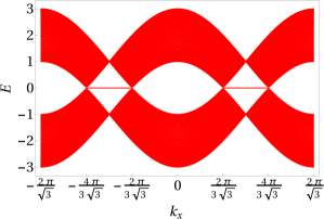
(a)

Figure 2: (color online) Band structure of zigzag ribbon for a pristine graphene.

To see how the states at edges look like, we have plotted the probability density, $|\psi|^{2}$ as a function $n$ by solving the Eq. 4 and present them in Fig. 3 (a). It shows that the wavefunction has maximum amplitudes at the edges and gradually decays as one moves inwards. The lack of a gap in pristine graphene turns the $E=0$ state into a resonance whose amplitude decays [50]. To compare the analytical results with numerical ones, we have plotted the local density of states (LDOS) in Fig. 3 (b) for energy value close to zero. It can be seen that the LDOS is largest at the edges and falls off gradually into the bulk. Thus these edge states are conducting in nature, whereas deep inside the bulk remains insulating owing to its decaying amplitude.

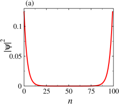
(a)

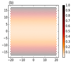
(b)

Figure 3: (color online) (a) Probability density of the wavefunction, $|\psi|^{2}$ as a function of $n$ and (b) the LDOS plot for pristine graphene.

To ascertain the effects of edge modes on the conductance properties of a KMNR, we have computed the conductance of pristine (zigzag) graphene as shown in Fig. 4. The conductance behavior shows that a $2e^{2}/h$ plateau exists around the zero of the Fermi energy which is shown by the black dotted line. However, this plateau is fragile owing to the absence of ‘protected’ edge states.

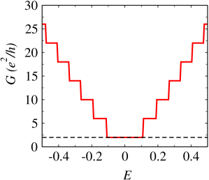
(a)

Figure 4: (color online) The charge conductance, $G$ (in units of $e^{2}/h$) is plotted as a function of energy $E$ (in units of $t$) for pristine graphene.

5.2 Intrinsic SOC

In this subsection, we shall discuss results for an intrinsic SOC added to a pristine graphene. Fig. 5 shows the band structure with two different intrinsic SO coupling strengths, namely $t_{2}=0.1$ and 0.5. The system dimensions have been kept the same as that in pristine graphene. Now from fig. 5 (a), we see a gap has opened at the Dirac points which may appear that the system is a spin Hall insulator (SHI) [51] with edge modes. As shown in Fig. 5 (b), a larger gap than the previous case is observed. To confirm the existence of edge modes, we have also plotted the probability density and local density of states (LDOS) as shown in Fig. 6.

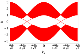
(a)

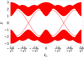
(b)

Figure 5: (color online) Band structure of zigzag graphene ribbon with coupling parameter (a) $t_{2}=0.1$ and (b) $t_{2}=0.5$.

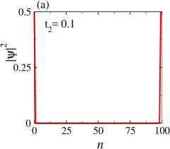
(a)

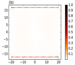
(b)

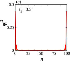
(c)

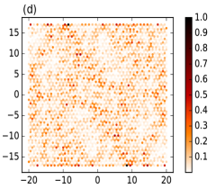
(d)

Figure 6: (Color online) Probability density of the wave-function, $|\psi|^{2}$ as a function of $n$ for (a) $t_{2}=0.1$ and (c) $t_{2}=0.5$. The LDOS plot for (b) $t_{2}=0.1$ and (d) $t_{2}=0.5$. Here $\lambda_{R}$ is not considered.

We have plotted the probability density for the edge states with the strength of the intrinsic coupling, $t_{2}=0.1$ as shown in Fig. 6 (a). Now the edge states fall off sharply on both sides of the sample. We have also plotted the LDOS for the comparison. The corresponding Fig. 6 (b) implies that the electronic states are highly localized at the edges and are zero immediately inwards. However, the inclusion of the intrinsic SOC respects the time reversal symmetry of the Kane-Mele Hamiltonian and hence these edge states should be protected by topological invariance. We have also plotted the probability amplitude in Fig. 6 (c) and the LDOS in Fig. 6 (d) for a larger intrinsic SOC, namely $t_{2}=0.5$ . The probability amplitude now does not decay sharply as that for $t_{2}=0.1$ and also this result is in agreement with the LDOS plot where the states are not localized at the edges of the sample rather show an oscillating nature. The localized edge states as seen from Fig. 6 (a) and Fig. 6 (b) conduct and should yield a non-zero conductance value at zero bias.

To see this we have plotted the (charge) conductance, $G$ as a function of Fermi energy, $E$ in presence of the intrinsic SOC as shown in Fig. 7. Although the step-like behavior is absent unlike that of pristine graphene, a $2e^{2}/h$ plateau is still observed for the case of $t_{2}=0.1$ shown by the black dotted line in Fig. 7 (a). However, for $t_{2}=0.5$ as shown in Fig. 7 (b), there is no $2e^{2}/h$ plateau near the zero of the Fermi energy. It is also important to note that the maximum value of the conductance, that is at $|E|\simeq 0.5$ is higher for lower values of the intrinsic SOC.

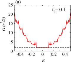
(a)

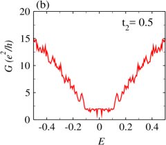
(b)

Figure 7: (color online) The charge conductance, $G$ (in units of $e^{2}/h$) is plotted as a function of energy E (in units of $t$) for (a) $t_{2}=0.1$ and (b) $t_{2}=0.5$. We have considered $\lambda_{R}=0$

5.3 Rashba SOC

Next we add a Rashba spin orbit coupling to a pristine graphene. Thus here we have $t_{2}=0$, but $\lambda_{R}\neq 0$. For a small value of $\lambda_{R}$, the flat band is observed in Fig. 8 (a) as we have seen in pristine graphene. However, if we enhance $\lambda_{R}$, the flat band reduces as shown in Fig. 8 for a large value of $\lambda_{R}$, namely $\lambda_{R}=0.5$, where the flat bands have almost vanished and in the $|k_{x}|$ range of $\left[\frac{2\pi}{3\sqrt{3}}:\frac{4\pi}{3\sqrt{3}}\right]$.

(a)

(b)

Figure 8: (color online) Band structure of zigzag ribbon for (a) $\lambda_{R}=0.1$ and (b) $\lambda_{R}=0.5$. Here $t_{2}=0$.

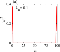
(a)

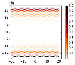
(b)

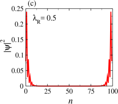
(c)

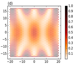
(d)

Figure 9: (Color online) Probability density of the wave-function, $|\psi|^{2}$ as a function of $n$ for (a)$\lambda_{R}=0.1$ and (b) $\lambda_{R}=0.5$. The LDOS plot for (c) $\lambda_{R}=0.1$ (d) $\lambda_{R}=0.5$. The oscillatory pattern is seen in (c) and (d).

The above features are appropriately justified by the analytic behavior (obtained by solving Eq. 7 by putting $t_{2}=0$) as shown in Fig. 9. For small values of $\lambda_{R}$, there is no oscillation and the probability density decay quickly as one moves inward as shown in Fig. 9 (a). The corresponding LDOS plot in Fig. 9 (b) shows the same behavior. For large values of $\lambda_{R}$, the probability densities show damped oscillations as one moves inside the bulk, and remain finite till quite a few lattice spacings inside the sample. The LDOS plots in Fig. 9 (d) provides ample support for this oscillatory behavior and non-vanishing weights inside the bulk.

Finally, we have plotted the charge conductance as shown in Fig. 10. For $\lambda_{R}=0.1$, there is a $2e^{2}/h$ plateau near the zero of the Fermi energy as shown in Fig. 10 (a). However, this $2e^{2}/h$ value is not associated with a topological phase as is evident from Fig. 9. The conductance as a function of energy shows the absence of plateau at a $2e^{2}/h$ and closing of gaps are observed near the zero of the Fermi energy in Fig. 10 (b). These results signify the absence of edge modes and subsequently any topologically non-trivial behavior in the conductance data.

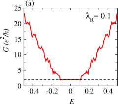
(a)

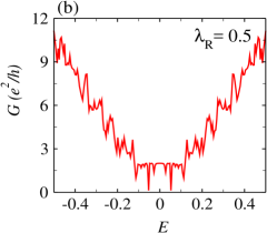
(b)

Figure 10: (color online) The charge conductance, $G$ (in units of $e^{2}/h$) is plotted as a function of energy $E$ (in units of t) for (a) $\lambda_{R}=0.1$ and (b) $\lambda_{R}=0.5$

5.4 Intrinsic and Rashba SOC

In this section, we include both the intrinsic and the Rashba SOC in the graphene nanoribbon and call this as Kane-Mele nanoribbon (KMNR) with zigzag edges. It is sensible to ask what happens to the edge state when both are present. The Kane-Mele Hamiltonian is P-T symmetric and the Kramer’s doublet must enjoy topological protection. However, the existence of edge states still needs to be ascertained and the implications on the conductance spectra thereof.

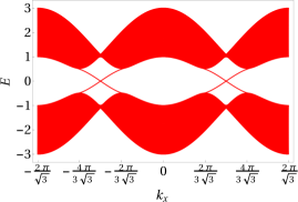
(a)

(b)

Figure 11: (color online) The band structure of zigzag KMNR with (a) $t_{2}=0.1$ and $\lambda_{R}=0.01$ (b) $t_{2}=0.1$ and $\lambda_{R}=0.2$.

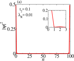
(a)

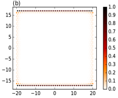
(b)

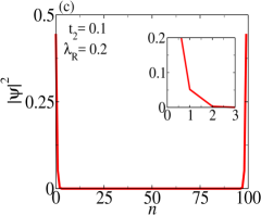
(c)

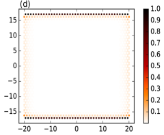
(d)

Figure 12: (color online) (a) Probability density of the wave-function, $|\psi|^{2}$ as a function of $n$ and (b) the corresponding LDOS plot for $t_{2}=0.1$,$\lambda_{R}=0.01$. (c) and (d) is plotted for $t_{2}=0.1$ and $\lambda=0.2$.

We keep $t_{2}=0.1$ and explore two values of Rashba SOC, namely, $\lambda_{R}=0.01$ and $\lambda_{R}=0.2$. The former corresponds to $\lambda_{R}<t_{2}$ $(<t)$ and the latter denote $\lambda_{R}>t_{2}$ $(<t)$. The band structures for the corresponding cases are shown in Fig. 11. When the strength of the Rashba SOC is weak, the band structure for $t_{2}=0.1$ is almost similar (shown in Fig. 11 (a)) with the band structure for the same value of the intrinsic SOC in the absence of Rashba coupling (Fig. 5 (a)). However, for a higher value of $\lambda_{R}$ (Fig. 11 (b)), the band gap gets smaller than the previous case. The results corresponding to the two cases are not much different with regard to the existence of the edge states. The only (minor) difference is that the analytic form yields a non-zero value for $n=2$ corresponding to the larger value of $\lambda_{R}$, that is, $\lambda_{R}=0.2$. The LDOS maps corroborate existence of edge modes (see Fig. 12 (b) and (d)) as is evident for Fig. 12 (a) and (c).

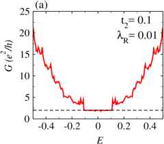
(a)

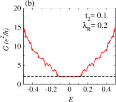
(b)

Figure 13: (color online) The charge conductance, $G$ (in units of $e^{2}/h$) is plotted as a function of energy $E$ (in units of t) for $t_{2}=0.1$ and $\lambda_{R}=0.2$.

The conductance plots as a function of the Fermi energy in Fig. 13 show the existence of a $2e^{2}/h$ plateau, which are topologically protected and correspond to quantum spin Hall insulating phase. It may be noted that we have presented plots only for two sets of parameter values, namely ($t_{2}$, $\lambda_{R}$) = (0.1, 0.01) and (0.1, 0.2). However, the same inferences can be drawn for other sets, such as larger values of $t_{2}$ and $\lambda_{R}$ which we have explicitly checked, but have not shown the data for brevity.

Conclusions

In this paper, we have analytically computed expressions for the edge modes for a Kane-Mele nanoribbon (KMNR). The analytic results are supported by LDOS obtained using KWANT. Further, we have calculated the band structure and conductance for a pristine graphene, graphene with intrinsic SOC, graphene with Rashba SOC and graphene with both SOCs. We re-establish the existence of topologically protected edge states owing to the presence of parity and time reversal symmetry of the Hamiltonian. The system acquires edge states in presence of spin orbit couplings as observed from band structure and both analytic and numeric calculation of electron probability densities. The conductance spectra further show a plateau at a non-zero value $(=2e^{2}/h)$ near the zero of the Fermi energy.

References

- [1] K. S. Novoselov, A. K. Geim, S. V. Morozov, D. Jiang, Y. Zhang, S. V. Dubonos, V. Grigoreva, and A. A. Firsov, Science 306, 666 (2004).
- [2] P. R. Wallace, Phys. Rev. 71, 622 (1947).
- [3] A. H. C. Neto, F. Guinea, N. M. R. Peres, K. S. Novoselov, and A. K. Geim, Rev. Mod. Phys. 81, 109 (2009).
- [4] Y. Zhang, Y.-W. Tan, H. L. Stormer, and P. Kim, Nature 438, 201 (2005).
- [5] V. P. Gusynin and S. G. Sharapov, Phys. Rev. Lett. 95, 146801 (2005).
- [6] E-J. Kan, Z. Li, J. Yang, and J. G. Hou, Appl. Phys. Lett. 91, 243116 (2007).
- [7] X. Lin and J. Ni, Phys. Rev. B 84, 075461 (2011).
- [8] M. I. Katsnelson , K. S. Novoselov, and A. K. Geim Nat. Phys. 2 620 (2006).
- [9] X. Du, I. Skachko, A. Barker, and E. Y. Andrei, Nat. Nanotech. 3 491 (2008).
- [10] K. I. Bolotin , K. J. Sikes , J. Hone, H. L. Stormer, and P. Kim, Phys. Rev. Lett. 101 096802 (2008).
- [11] B. I. Halperin, Phys. Rev. B 25, 2185 (1982).
- [12] R. B. Laughlin, Phys. Rev. B 23, 5632 (1981).
- [13] C. L. Kane and E. J. Mele, Phys.Rev.Lett. 95, 226801 (2005).
- [14] C. L. Kane and E. J. Mele, Phys.Rev.Lett. 95, 146802 (2005).
- [15] B. A. Bernevig and S.-C. Zhang, Phys. Rev. Lett. 96, 106802 (2006).
- [16] B. A. Bernevig, T. L. Hughes, and S.-C. Zhang, Science 314, 1757 (2006).
- [17] C. Wu, B. A. Bernevig, and S.-C. Zhang, Phys. Rev. Lett. 96, 106401 (2006).
- [18] M. Onoda and N. Nagaosa, Phys. Rev. Lett. 95, 106601 (2005).
- [19] J. E. Moore, Nature (London) 464, 194(2010).
- [20] M. Z. Hasan and C. L. Kane, Rev. Mod. Phys. 82, 3045 (2010).
- [21] X.-L. Qi and S.-C. Zhang, Rev. Mod. Phys. 83, 1057 (2011).
- [22] H. Min, J. E. Hill, N. A. Sinitsyn, B. R. Sahu, L. Kleinman, and A. H. MacDonald, Phys.Rev.B 74, 165310( 2006).
- [23] Y. G. Yao, F. Ye, X.-L. Qi, S.-C. Zhang, and Z. Fang, Phys. Rev.B 75, 041401 (2007).
- [24] M. König, S. Wiedmann, C. Brüne, A. Roth, H. Buhmann, L. W. Molenkamp, and X-L. Qi, S-C. Zhang, Science 318, 766 (2007).
- [25] C. Weeks, J. Hu, J. Alicea, M. Franz, and R. Wu, Phys.Rev. X 1, 021001 (2011).
- [26] L. Kou, B. Yan, F. Hu, S.-C. Wu, T. O. Wehling, C. Felser, C. Chen, and T. Frauenheim, Nano Lett. 13, 6251 (2013).
- [27] J. Zhang, C. Triola, and E. Rossi, Phys. Rev. Lett. 112, 096802 (2014).
- [28] K. Zollner, T. Frank, S. Irmer, M. Gmitra, D. Kochan, and J. Fabian, Phys. Rev. B 93, 045423 (2015).
- [29] D. Marchenko, A. Varykhalov, M. Scholz, G. Bihlmayer, E.I. Rashba, A. Rybkin, A.M. Shikin, and O. Rader, Nat. Commun. 3, 1232 (2012).
- [30] Y. S. Dedkov, M. Fonin, U. Rüdiger, and C. Laubschat, Phys. Rev. Lett. 100, 107602 (2008).
- [31] F. Calleja, H. Ochoa, M. Garnica, S. Barja, J. J. Navarro, A. Black, M. M. Otrokov, E. V. Chulkov, A. Arnau, A. L. V. de Parga, F. Guinea, and R. Miranda, Nat. Phys. 11, 43 (2015).
- [32] R. Seshadri, K. Sengupta, and D. Sen, Phys. Rev. B 93, 035431 (2016).
- [33] K. Nakada, M. Fujita, G. Dresselhaus, and M. S. Dresselhaus, Phys. Rev. B 54, 17954 (1996).
- [34] K. Wakabayashi, M. Fujita, H. Ajiki, and M. Sigrist, Phys. Rev. B 59, 8271 (1999).
- [35] K. Wakabayashi, M. Sigrist, and M. Fujita, J. Phys. Soc. Japan 67, 2089 (1998).
- [36] M. Laubach, J. Reuther, R. Thomale, and S. Rachel, Phys. Rev. B 90, 165136 (2014).
- [37] D. Huertas-Hernando, F. Guinea, and A. Brataas, Phys. Rev. B 74, 155426 (2006).
- [38] is a number such that is bounded between . Here we have taken = 2.15.
- [39] R. Seshadri and D. Sen, J. Phys. Condens. Matter 29, 155303 (2017).
- [40] Z-F.Liu, Q-P. Wu, A-X. Chen, X-B. Xiao, N.H. Liu, and G-X. Miao, Scientific reports (2017).
- [41] M. Zarea and N. Sandler, Phys. Rev. B 79, 165442 (2009).
- [42] R. Landauer, IBM J. Res. Dev. 1, 223 (1957).
- [43] R. Landauer, Philos. Mag. 21, 683 (1970).
- [44] C. Caroli, R. Combescot, P. Nozieres, and D. Saint-James, J. Phys C: Solid State Phys. 4, 916, (1971).
- [45] D. S. Fisher and P. A. Lee, Phys. Rev. B 23, 6851 (1981).
- [46] S. Datta, Electronic transport in Mesoscopic systems, University press (Cambridge), (1995).
- [47] B. K. Nikolić, Phys. Rev. B 64, 014203 (2001).
- [48] C. W. Groth, M. Wimmer, A. R. Akhmerov, and X. Waintal, New J. Phys. 16, 063065 (2014).
- [49] (Width , length with KMNR dimensions ) S. Ganguly and S. Basu, Mater. Res. Express 4, 11 (2017).
- [50] J. Lado, N. Garcia-Martinez, and J. Fernandez-Rossier, Synth. Met. 210, 56 (2015).
- [51] S. Murakami, N. Nagaosa, and S.-C. Zhang, Phys. Rev. Lett. 93, 156804 (2004).