Adversarial Regression for Detecting Attacks in Cyber-Physical Systems

Abstract

Attacks in cyber-physical systems (CPS) which manipulate sensor readings can cause enormous physical damage if undetected. Detection of attacks on sensors is crucial to mitigate this issue. We study supervised regression as a means to detect anomalous sensor readings, where each sensor’s measurement is predicted as a function of other sensors. We show that several common learning approaches in this context are still vulnerable to stealthy attacks, which carefully modify readings of compromised sensors to cause desired damage while remaining undetected. Next, we model the interaction between the CPS defender and attacker as a Stackelberg game in which the defender chooses detection thresholds, while the attacker deploys a stealthy attack in response. We present a heuristic algorithm for finding an approximately optimal threshold for the defender in this game, and show that it increases system resilience to attacks without significantly increasing the false alarm rate.

1 Introduction

Cyber-physical systems (CPS) form the foundation of much of the critical infrastructure, including the electric power grid, transportation networks, water networks, and nuclear plants, among others. Malicious attacks on CPS can consequently lead to major disruptions, from major blackouts to nuclear incidents. Moreover, such attacks are no longer hypothetical, with Stuxnet perhaps the best-known example of an attack targeting physical infrastructure through cyber means. A crucial aspect of the Stuxnet attack—and a feature that is central to most attacks on CPS—is the corruption of sensor readings to either ensure that an attack on the controller code is undetected, or indirectly impact controller behavior. The power of sensor corruption to impact control decisions is particularly alarming: since controllers are commonly making decisions directly as a consequence of readings from critical sensors, for example, increasing or decreasing temperature to ensure it stays within a target (safe) range, tampering with these readings (e.g., temperature) can cause the controller itself to put the system into an unsafe state. With no remediation, as soon as a critical sensor is compromised, the attacker can cause major system failure by directly manipulating sensor measurements in essentially arbitrary ways.

Data-driven anomaly detection techniques have previously been proposed to mitigate against arbitrary manipulations of sensor data, both based on temporal statistics of single-sensor measurements Ghafouri et al. (2016), as well as by modeling joint measurements to obtain a prediction for each sensor based on measurements of others Ghafouri et al. (2017). However, these have been limited in two ways: 1) they generally consider a specific anomaly detection method, such as a Gaussian Process regression, and 2) they do not consider attacks which can arbitrarily modify a collection of sensor measurements.

To address these limitations, we present a general framework for adversarial anomaly detection in the context of integrity attacks on a subset of sensors in CPS. We start with a general anomaly detection framework based on a collection of supervised regression models which predict a measurement for each sensor as a function of readings from other sensors. We instantiate this framework with three regression models: linear regression, neural network, and an ensemble of the two. We then develop an optimization approach for stealthy attacks on linear regression which aim to maximally increase or decrease a reading for a collection of target sensors (for example, those serving as direct inputs into a controller which maintains the system in a safe state), and extend these to consider a neural network detector, and the ensemble of these.

Next, we model robust anomaly detection as a Stackelberg game between the defender who chooses detection thresholds for each sensor to balance false alarms with impact from successful attacks, and the attacker who subsequently deploys a stealthy attack. Finally, we develop a heuristic algorithm to compute a resilient detector in this model. Our experiments show that (a) the stealthy attacks we develop are extremely effective, and (b) our resilient detector significantly reduces the impact of a stealthy attack without appreciably increasing the false alarm rate.

Related Work

A number of techniques have been proposed for anomaly detection in CPS, aimed at identifying either faults or attacks. Several of these consider simplified mathematical models of the physical system, rather than using past data of normal behavior to identify anomalies Cárdenas et al. (2011); Urbina et al. (2016). A number of others use statistical and machine learning techniques for anomaly detection Nader et al. (2014); Junejo and Goh (2016); Ghafouri et al. (2016, 2017), but restrict attention to a specific model, such as Gaussian Process regression Ghafouri et al. (2017), to a single sensor Ghafouri et al. (2016), to unsupervised techniques Nader et al. (2014), or to directly predict attacks based on normal and simulated attack data Junejo and Goh (2016). Ours is the first approach which deals with a general framework for regression-based modeling of sensor readings based on other sensors.

In addition, considerable literature has developed around the general problem of adversarial machine learning, which considers both attacks on machine learning methods and making learning more robust Lowd and Meek (2005); Dalvi et al. (2004); Biggio et al. (2014); Li and Vorobeychik (2014); Vorobeychik and Li (2014); Li and Vorobeychik (2018). However, all focus on inducing mistakes in a single model—almost universally, a classifier (Grosshans et al. [2013] is a rare exception). In contrast, we study stealthy attacks on sensor readings, where even the critical measurement can be manipulated directly, but where multiple models used for anomaly detection impose strong constraints on which sensor manipulations are feasible. As such, our framework is both conceptually and mathematically quite different from prior research on adversarial learning.

2 Regression-Based Anomaly Detection

Consider a collection of $d$ sensors, with $y$ representing a vector of sensor measurements, where $y_{s}$ is the measurement of a sensor $s$. In practice, such measurements often feed directly into controllers which govern the state of critical system components. For example, such a controller may maintain a safe temperature level in a nuclear reactor by cooling the reactor when the temperature reading becomes too high, or heating it when it’s too low. If an attacker were to take control of the sensor which measures the temperature of the nuclear reactor, they can transmit low sensor readings to the controller, causing it to heat up the reactor to a temperature arbitrarily above a safe level!

A way to significantly reduce the degree of freedom available to the attacker in this scenario is to use anomaly detection to identify suspicious measurements. To this end, we can leverage relationships among measurements from multiple sensors: if we can effectively predict a reading from a sensor based on the measurements of others, many sensors would need to be compromised for a successful attack, and even then the attacker would face complex constraints in avoiding detection: for example, slightly modifying the one sensor may actually cause another sensor to appear anomalous.

Table 1: List of Symbols

Symbol	Description
$S$	Set of sensors
$y_{s}$	Actual measurement of sensor $s$
$\tilde{y}_{s}$	Observed measurement value of sensor $s$ after the attack
$r_{s}$	residual of sensor $s\in S$
$S_{c}$	Set of critical sensors
$\delta_{s}$	Error added to sensor $s\in S$
$B$	The maximum number of sensors that can be attacked (attacker’s budget)
$D$	Set of sensors with detectors
$f_{s}$	Regression-based predictor of detector $s\in D$
$\tau_{s}$	Threshold value of detector $s\in D$

We therefore propose the following general framework for anomaly detection in a multi-sensor CPS. For each sensor $s$, we learn a model $f_{s}(y_{-s})$ which maps observed readings from sensors other than $s$ to a predicted measurement of $s$. Learning can be accomplished by collecting a large amount of normal system behavior for all sensors, and training the model for each sensor. At operation time, we can then use these predictions, together with observed measurements, to check for each sensor $s$ whether its measurement is anomalous based on residual $r_{s}=|f_{s}(y_{-s})-y_{s}|$, and a threshold $\tau_{s}$, where $r_{s}\leq\tau_{s}$ is considered normal, while $r_{s}>\tau_{s}$ is flagged as anomalous. For easy reference, we provide the list of these and other symbols used in the paper in Table 1.

In principle, any supervised learning approach can be used to learn the functions $f_{s}$. We consider three illustrative examples: linear regression, neural network, and an ensemble of the two.

Linear Regression

In this case, for each detector $s$, we let the predictor be a linear regression model defined as $f_{s}(y_{-s})=w_{s}^{T}y_{-s}+b_{s}$, where $w_{s}$ and $b_{s}$ are the parameters of the linear regression model.

Neural Network

In this case, for each sensor $s$, we let the predictor $f_{s}$ be a feed-forward neural network model defined by parameters $\theta_{s}$, where the prediction $f_{s}(y_{-s};\theta_{s})$ is obtained by performing a forward-propagation.

Ensemble

It has been shown in the adversarial learning literature that multiple detectors can improve adversarial robustness Biggio et al. (2010). We explore this idea for the ML regression-based detector by considering an ensemble model for the predictor. We consider an ensemble predictor that contains a neural network and a linear regression model. Different methods can be used for combining the results, but we consider a bagging approach where the result is computed as the average of the predictors’ outputs.

3 Attacking the Anomaly Detector

We have informally argued above that the anomaly detector makes successful sensor manipulation attacks challenging. For example, the trivial attack on the critical sensors is now substantially constrained. We now study this issue systematically, and develop algorithmic approaches for stealthy attacks on sensors which attempt to optimally skew measured values of target sensors without tripping an anomaly detection alarm. While arbitrary changes to the sensor readings are no longer feasible, our experiments subsequently show that, unfortunately, a baseline anomaly detector is still quite vulnerable. Subsequently, we develop an approach for making it more robust to stealthy attacks.

3.1 Attacker Model

We define the attack model by describing the attacker’s capability, knowledge, and objective. Capability: The adversary may compromise and make arbitrary modifications to the readings from up to $B$ sensors. Knowledge: We consider a worst-case scenario where the attacker has complete knowledge of the system and anomaly detectors. Objective: The attacker’s objective is to maximize or minimize the observed value for some critical sensor $\bar{s}$ among a collection of target sensors $S_{c}$. In addition, the attacker’s modifications to the sensors it compromises must remain undetected (stealthy) with respect to the anomaly detection model.

Formally, let $\tilde{y}$ be the sensor measurements observed after the attacker compromises a subset of sensors. We assume that the attacker can compromise at most $B$ sensors; consequently, for the remaining $d-B$ sensors, $\tilde{y}_{s}=y_{s}$. Additionally, the attacker cannot modify individual measurements of compromised sensors arbitrarily (for example, constrained by sensor-level anomaly detectors), so that $|\tilde{y}_{s}-y_{s}|\leq\eta_{s}$; $\eta_{s}=\infty$ is then a special case in which the attacker is not so constrained. The final set of constraints faced by the attacker ensures that the attack is stealthy: that is, it doesn’t trigger alerts based on the anomaly detection model described in Section 2. To accomplish this, the attacker must ensure that for any sensor $s$, $|\tilde{y}_{s}-f_{s}(\tilde{y}_{-s})|\leq\tau_{s}$, that is, the corrupted measurements must simultaneously appear normal with respect to the detector model described above and observed measurements $\tilde{y}_{s}$ for all sensors (both attacked, and not). Note that this is a subtle constraint, since corrupted measurements for one sensor may make another appear anomalous.

For a given critical sensor $\bar{s}$, the attacker’s goal is to maximize or minimize the corrupted measurement $\tilde{y}_{\bar{s}}$. Here we focus on minimization of observed values of critical sensors; approaches where the goal is to maximize these values are essentially the same. The attacker’s optimization problem is then

$$\operatorname*{argmin}_{\bar{s}\in S_{c}}\; \min_{\tilde{y}}\tilde{y}_{\bar{s}}$$

s.t. $$|\tilde{y}_{s}-f_{s}(\tilde{y}_{-s})|\leq\tau_{s},\forall s\in D$$ (1a)

$$|\tilde{y}_{s}-y_{s}|\leq\eta_{s},\forall{s}$$ (1b)

$$\left\lVert\tilde{y}-y\right\rVert_{0}\leq B,$$ (1c)

where Constraints (1a) capture evasion of the anomaly detector (to ensure that the attack is stealthy), Constraints (1b) limit modifications of individual sensors, if relevant, and Constraint (1c) limits the attacker to attack at most $B$ sensors.

Not surprisingly, the problem faced by the adversary is NP-Hard.

Proposition 1.

The Adversarial Regression Problem is NP-Hard.

The proof of this proposition is in the appendix.

Despite the hardness result, we now present algorithmic approaches for solving Problem (1) in the context of linear regression and neural networks, as well as a simple ensemble of these described in Section 2.

3.2 Attacking Linear Regression

First, we replace the non-convex budget constraint using a collection of linear constraints. Define $\alpha_{s}$ as a binary variable indicating whether the sensor $s$ is attacked. Thus, Constraint (1c) can be re-written as $\sum_{i=1}^{m}\alpha_{i}\leq B$. Now, for each sensor $s$ let $\tilde{y}_{s}=y_{s}+\delta_{s}$, where $\delta_{s}$ represents the modification made by the adversary. Since $\delta_{s}>0$ only if $s$ has been compromised (i.e., $\alpha_{s}=1$), we add a constraint $\delta_{s}\leq M\alpha_{s}$ where $M$ is a sufficiently large number.

Next, we rewrite Constraints (1a). In the case of a linear regression model for anomaly detection, Constraints (1a) become $|\tilde{y}_{s}-w_{s}^{T}\tilde{y}_{-s}-b_{s}|\leq\tau_{s}$. These can be represented using two sets of linear constraints: $\tilde{y}_{s}-w_{s}^{T}\tilde{y}_{-s}-b_{s}\leq\tau_{s}$ and $-\tilde{y}_{s}+w_{s}^{T}\tilde{y}_{-s}+b_{s}\leq\tau_{s}$. Finally, Constraints (1b) are similarly linearized as $\delta_{s}\leq\eta_{s}$ and $-\delta_{s}\leq\eta_{s}$.

Putting everything together, we obtain the following mixed-integer linear programming (MILP) problem (actually, a minimum over a finite number of these), which solves problem (1) for the linear regression-based anomaly detector:

$$\operatorname*{argmin}_{\bar{s}\in S_{c}}\; \min_{\tilde{y},\delta,\alpha}\delta_{\bar{s}}$$

s.t. $$\tilde{y}_{s}-w_{s}^{T}\tilde{y}_{-s}-b_{s}\leq\tau_{s},\forall{s}$$ (2a)

$$-\tilde{y}_{s}+w_{s}^{T}\tilde{y}_{-s}+b_{s}\leq\tau_{s},\forall{s}$$ (2b)

$$\tilde{y}_{s}=y_{s}+\delta_{s},\forall{s}$$ (2c)

$$\delta_{s}\leq M\alpha_{s},\forall{s}$$ (2d)

$$\delta_{s}\leq\eta_{s};\ -\delta_{s}\leq\eta_{s},\forall{s}$$ (2e)

$$\sum_{s}\alpha_{s}\leq B$$ (2f)

$$\tilde{y}_{s},\delta_{s}\in\mathbb{R},\alpha_{s}\in\{0,1\}\ \forall{s}.$$

3.3 Attacking Neural Network Regression

Due to the non-linear structure of a neural network model, Constraints (1a) now become non-linear and non-convex. To tackle this challenge (1), we propose an iterative algorithm, described in Algorithm 1. The algorithm solves the problem by taking small steps in a direction of increasing objective function. In each iteration, the algorithm linearizes all the neural networks at their operating points, and replaces them with the obtained linearized instances. Then, for each small step, it solves the MILP (2) to obtain an optimal stealthy attack in the region around the operating point. In each iteration, in order to ensure that the obtained solution is feasible, the algorithm tests the solution with respect to the actual neural network-based anomaly detectors. If it is infeasible, the iteration is repeated using a smaller step size. Otherwise, the same process is repeated until a local optimum is found or we reach a desired maximum number of iterations.

Algorithm 1 Adversarial Regression for Neural Network

1:Input: Measurements $\tilde{y}$, critical sensors $S_{c}$, budget $B$, algorithm parameters $\epsilon_{0}$, $n_{max}$

2:$\tilde{y}_{0}\leftarrow\tilde{y}$, $\delta_{\bar{s}^{\ast}}\leftarrow 0$

3:for all $\bar{s}\in S_{c}$ do

4:    while number of iterations $<n_{max}$ and $\epsilon>\epsilon_{min}$ do

5:         // Linearize all neural networks at $\tilde{y}$

6:        $[W,b]\leftarrow$TaylorApproximation($f_{s}(\cdot),\tilde{y}$)

7:         // Solve MILP and check feasibility

8:        $\epsilon\leftarrow\epsilon_{0}$

9:        $\tilde{y}^{\prime}\leftarrow$Solve_MILP($W$,$b$,$\bar{s}$,$\tilde{y}$,$\epsilon$)

10:        for each sensor $s$ do

11:           if $|\tilde{y}^{\prime}_{s}-f^{(s)}(\tilde{y}^{\prime}_{-s})|>\tau_{s}$ then

12:               $\epsilon\leftarrow\frac{\epsilon}{2}$

13:               go to Line 9

14:           end if

15:        end for

16:        $\tilde{y}\leftarrow\tilde{y}^{\prime}$

17:        $\delta_{\bar{s}}\leftarrow\tilde{y}^{\prime}_{\bar{s}}$

18:    end while

19:    if $\delta_{\bar{s}^{\ast}}<\delta_{\bar{s}}$  then

20:        $\bar{s}^{\ast}\leftarrow\bar{s}$, $\delta_{\bar{s}^{\ast}}\leftarrow\delta_{\bar{s}}$, $\tilde{y}^{\ast}\leftarrow\tilde{y}$

21:    end if

22:end for

23:return $\tilde{y}^{\ast}$

The algorithm begins with the initial uncorrupted measurement vector $\tilde{y}=y$. For each neural network $f_{s}$, it obtains a linearized model using a first-order Taylor expansion around the solution estimate $\tilde{y}$ in the current iteration, which yields a matrix of weights $W$ for the corresponding linear approximation. Given matrix $W$, we solve the problem by converting it to the MILP (2), with a small modification: we introduce a constraint that enforces that we only make small modifications relative to the approximate solution from the previous iteration. More precisely, we let $\epsilon\in\mathbb{R}_{+}$ be the parameter representing the maximum step size. Then, we add the constraint $|\Delta|<\epsilon$ to the MILP, where $\Delta=y+\delta-\tilde{y}$ and $\tilde{y}$ the latest solution.

Let $\tilde{y}^{\prime}$ be the solution obtained by solving the MILP. We check whether this solution is feasible by performing forward-propagation in all the neural networks and checking that no stealth constraint is violated. If a stealth constraint is violated, which means that our linearized model was not a good approximation of the neural network, we discard the candidate solution, reduce the maximum step size parameter $\epsilon$ to improve the approximation, and re-solve the MILP. We repeat this process until a feasible solution is found, in which case the same steps are repeated for a new operating point, or until we reach the maximum number of iterations $n_{max}$. Finally, we check whether the solution that is found for the current target sensor $\bar{s}$ outperforms the solution for the best target sensor found so far. The algorithm terminates after considering all the target sensors and returns the best attack vector found.

3.4 Attacking the Ensemble Model

We can view the ensemble as a single neural network that connects a perceptron (i.e., the linear regression model) with our initial neural network at the output layer. Thus, to solve the adversarial regression problem, we can use the same approach as in the case of neural networks by modifying Algorithm 1 to obtain linear approximation parameters $W=\frac{1}{2}(W_{NN}+W_{LR})$ and $b=\frac{1}{2}(b_{NN}+b_{LR})$, where $W_{LR}$ and $b_{LR}$ are the parameters of the linear regression model in the ensemble, and $W_{NN}$ and $b_{NN}$ the parameters of the Taylor approximation of the neural network piece of the ensemble.

4 Resilient Detector

Having developed stealthy attacks on the anomaly detection system we described earlier, we now consider the problem of designing robustness into such detectors. Specifically, we allow the defender to tune the thresholds $\tau_{s}$ to optimize robustness, accounting for stealthy attacks. More precisely, we model the game between the defender and attacker as a Stackelberg game in which defender first commits to a collection of thresholds $\tau_{s}$ for the anomaly detectors, and the attacker then computes an attack following the model in Section 3. The defender aims to minimize the impact of attacks $D(\tilde{y}(\tau))$, subject to a constraint that the number of false alarms is within $\gamma$ of that for a baseline $\bar{\tau}$, typically set to achieve a target number of false alarms without consideration of attacks. The constraint reflects the common practical consideration that we wish to detect attacks without increasing the number of false alarms far beyond a target tolerance level. We seek a Stackelberg equilibrium of the resulting game, which is captured by the following optimization problem for the defender:

$$\begin{split}\min_{\tau}\max_{s\in S_{c}}&\quad D_{s}(\tilde{y}(\tau))\\ \mathrm{s.t.:}&\ \ FA(\tau)\leq FA(\bar{\tau})+\gamma,\tilde{y}(\tau)\ \mathrm{solves}\ \mathrm{Problem}~{}\eqref{eq:adv},\end{split}$$ (3)

where $FA(\tau)$ is the number of false alarms when the threshold vector is $\tau$.

Given thresholds $\tau$, we define the impact of attack on a sensor $s$ as the mean value of problem (1) over a predefined time period $T$: $D_{s}(\tilde{y})=\sum_{t=1}^{T}(\tilde{y}_{s}^{t}-y_{s}^{t})$. Similarly, we compute $FA(\tau)$ as the total number of false alarms over $T$ time steps: $FA(\tau)=\sum_{s}\sum_{t=1}^{T}1_{|y_{s}^{t}-f_{s}(y_{-s}^{t})|>\tau_{s}}$.

The key way to reduce the attack impact $D(\tilde{y}(\tau))$ is by decreasing detection threshold. This can effectively force the attacker to launch attacks that follow the behavior of the physical system more closely, limiting the impact of attacks. On the other hand, smaller values of the threshold parameters may result in a higher number of false alarms. Next, we present a novel algorithm for resilient detector threshold selection as defined in Problem (3).

Let $\tau$ be initialized based on a target number of false alarms. In each iteration, given threshold values $\tau$ computed in the previous iteration, we find the (approximately) optimal stealthy attack $\tilde{y}(\tau)$, with associated impact $D(\tilde{y}(\tau))$. Let $A^{\ast}$ be the set of critical sensors upon which the attack $\tilde{y}$ has the largest impact, and let $A_{min}$ be the set of sensors with the smallest stealthy attack impact. To reduce $D_{A^{\ast}}(\tilde{y}(\tau))$, we reduce $\tau_{\bar{s}}$ for each $\bar{s}\in A^{\ast}$. Then, to minimize the change in the number of false alarms, we increase the threshold $\tau_{s}$ for each $s\in A_{min}$ to compensate for the false alarms added by detectors of sensors in $A^{\ast}$. These steps are repeated until we reach a local optimum. We formalize this in Algorithm 2.

Algorithm 2 Resilient Detector

1:Initialize: Initial threshold setting $\bar{\tau}$, and initial $\epsilon$

2:$\tau^{\prime}=\tau=\bar{\tau}$

3:$\tilde{y}\leftarrow\textsc{Attack}(\tau)$

4:$I=\infty$

5:while number of iterations $<n_{max}$ do

6:    if $\max_{s\in S_{c}}D_{s}(\tilde{y})\leq I$ then

7:        $\tau\leftarrow\tau^{\prime}$

8:    else

9:        $\epsilon\leftarrow\frac{\epsilon}{2}$

10:    end if

11:    $I\leftarrow\max_{s\in S_{c}}D_{s}(\tilde{y})$

12:    $A^{\ast}\leftarrow\operatorname*{argmax}_{s\in S_{c}}D_{s}(\tilde{y})$

13:    $A_{min}\leftarrow\operatorname*{argmin}_{s\in S_{c}}D_{s}(\tilde{y})$

14:    for all $s\in A^{\ast}$ do

15:        $\tau_{s}^{\prime}\leftarrow\tau_{s}-\epsilon$

16:    end for

17:    $\Delta FP\leftarrow FP(\tau^{\prime})-FP(\tau)$

18:    for all $s\in A_{min}$ do

19:        $\tau_{s}^{\prime}\leftarrow FP_{s}^{-1}(FP_{s}(\tau_{s})-\frac{1}{|A_{min}|}\Delta FP)$

20:    end for

21:    $\tilde{y}\leftarrow\textsc{Attack}(\tau^{\prime})$

22:end while

23:return $\tau$

5 Experiments

We evaluate our contributions using a case study of the well-known Tennessee-Eastman process control system (TE-PCS) First, we design regression-based anomaly detectors for the critical sensors in the system (e.g., pressure of the reactor, level of the product stripper). Then, we consider scenarios where an adversary launches sensor attacks in order to drive the system to an unsafe state. Finally, we evaluate the resilience of the system against such attacks using baseline detectors and the proposed resilient detector.

5.1 Tennessee-Eastman Process Control System

We present a brief description of the Tennessee-Eastman Process Control System (TE-PCS). TE-PCS involves two simultaneous gas-liquid exothermic reactions for producing two liquid products Downs and Vogel (1993). The process has five major units: reactor, condenser, vapor-liquid separator, recycle compressor, and product stripper. The chemical process consists of an irreversible reaction which occurs in the vapor phase inside the reactor. Two non-condensible reactants A and C react in the presence of an inert B to form a non-volatile liquid product D. The feed stream 1 contains A, C, and trace of B; feed stream 2 is pure A; stream 3 is the purge containing vapors of A, B, and C; and stream 4 is the exit for liquid product D.

There are 6 safety constraints that must not be violated (e.g, safety limits for the pressure and temperature of reactor). These safety constraints correspond to 5 critical sensors: pressure, level, and temperature of the reactor, level of the product stripper, and level of the separator. Further, there are several control objectives that should be satisfied, e.g., maintaining process variables at desired values and keeping system state within safe operating conditions. The monitoring and control objectives are obtained using 41 measurement outputs and 12 manipulated variables.

We use the revised Simulink model of TE-PCS Bathelt et al. (2015). We consider the implementation of the decentralized control law as proposed by Ricker Ricker (1996). To launch sensor attacks against TE-PCS, we update the Simulink model to obtain an information flow in which the adversary receives all the sensor measurements and control inputs, solves the adversarial regression problem, and then adds the error vector to the actual measurements.

Figure 1 shows how a sensor attack may drive the system to an unsafe state. In this scenario, the pressure of the reactor exceeds 3000 kPa which is beyond the safety limit and can result in reactor explosion.

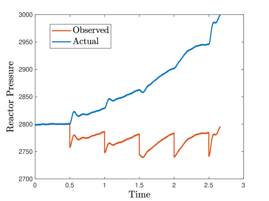
Figure 1: Pressure of the reactor when a sensor attack starts at $t=0.5$. After $2$ hours the pressure reaches an unsafe state.

5.2 Regression-Based Anomaly Detector

To protect the system against sensor attacks, we build a detector for each critical sensor. To train the detectors we run simulations that model the system operation for 72 hours, and collect the sensor measurements and control inputs. Each simulation consists of 7200 time steps and thus, for each simulation scenario, we record 7200$\times$53 datapoints. To make sure that the dataset represents different modes of operation, we repeat the same steps for different initial state values. We consider a total of 20 different initial state values which gives us 20$\times$7200$\times$53 $\approx$ 7.5 million datapoints.

Linear Regression-Based Detector

Using our collected data, we train linear regression models for the critical sensors. We use the current value of the remaining 36 non-critical sensors as well as the 9 non-constant control inputs as features of the model. Figure 2a shows the performance of the linear regression predictor on training and test data. Note that since the data is sequential, the train and test data cannot be randomly sampled and instead, we divide the data in two blocks. Also, to be able to compare the performance of predictors trained for different variables, we compute the MSE for normalized values instead of the actual values.

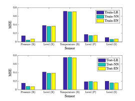
(a)

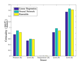
(b)

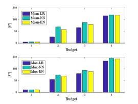
(c)

Figure 2: (a) MSE of Linear Regression, Neural Network, and Ensemble Model. All metrics are computed using Normalized Data. (b) Stealthy attack solution for the five critical sensors and different detectors. (c) Stealthy attack solution for the pressure of the reactor considering varying budgets.

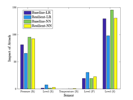
(a)

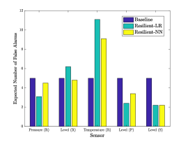
(b)

Figure 3: Resilient Detector for Linear Regression. (a) Impact of Resilient Detector compared to baseline. (b) False positive of Resilient Detector compared to baseline. (c) Trade-off between stealthy attack impact and false positive rate.

Neural Network-Based Detector

Next, we train the neural network regression models for the critical sensors. Unlike linear regression models, neural networks require several hyperparameters to be selected (e.g., network architecture, activation function, optimization algorithm, regularization technique). We considered neural networks with 2 to 4 hidden layers and 10 to 20 neurons in each layer. All the neurons in the hidden layers use tanh activation functions. We also experimented with ReLU activation functions but tanh performs better. We trained the networks in Tensorflow for 5000 epochs using Adam optimizer with $\beta_{1}=0.9$, $\beta_{2}=0.999$, and $\epsilon=10^{-8}$, and a learning rate of $0.01$. Figure 2a shows the MSE for training and test data, which outperforms the linear regression model. Finally, Figure 2a shows the result for the ensemble model.

5.3 Attacking Anomaly Detection

Figure 2b shows the attack solution for each critical sensor considering different detectors. As it can be seen, the temperature of the reactor is the least critical sensor while the level of the stripper is the most critical. Interestingly, neural network models, as well as ensembles, tend to be more vulnerable—often significantly—then the linear regression-based detectors. This is reminiscent of the observed vulnerability of neural network models to adversarial tampering Goodfellow et al. (2015), ours is the first observation that neural networks can be more fragile than simple linear models.

5.4 Resilient Detector

We use the resilient detector algorithm to find threshold values that reduce the stealthy attack impact as described in Section 4. We do this in the context of linear regression. Let $T^{\ast}=1$ hour, be the desired value for the expected time between false alarms for all detectors. As a baseline, for each detector $s$, we set threshold values $\tau_{s}=FP_{s}^{-1}(\frac{T^{\ast}}{d})$.

Then, we use Algorithm 2 to change thresholds in order to obtain better resilience. In the first iteration, stripper level is the most critical sensor, and reactor temperature the least critical. Therefore, we decrease the threshold corresponding to stripper level and increase the value of threshold for reactor temperature. We repeat these steps using Algorithm 2 until we obtain results shown in Figure 3. As we can see, we can significantly reduce the impact of the stealthy attack compared to the baseline (Figure 3a) without increasing the total number of false alarms (Figure 3b, where the total number of false alarms is the sum over all sensors).

6 Conclusions

We studied the design of resilient anomaly detection systems in CPS. We considered a scenario where the CPS is monitored by machine learning regression-based anomaly detectors, and an omniscient adversary capable of perturbing the values of a subset of sensors. The adversary’s objective is to lead the system to an unsafe state (e.g., raising the pressure of a reactor in a process control system beyond its safety limit) without being detected. We compute an optimal stealthy attack for linear regression, neural network, and a simple ensemble of these. Finally, we present an approach to mitigate the impact of stealthy attacks through resilient configuration of detector thresholds. We demonstrated the effectiveness of our methods using a case study of a process control system.

Appendix A Proof of Proposition 1

Definition 1 (Adversarial Regression Problem (Decision Version)).

Given an anomaly detector, a set of critical sensors $S_{c}$, an attack budget $B$, and a threshold attack $\tilde{y}_{c}^{\ast}$, determine whether there exists an attack with a value of at least $\tilde{y}_{c}^{\ast}$.

We prove this proposition using a reduction from a well-known NP-hard problem, the Maximum Independent Set Problem.

Definition 2 (Maximum Independent Set Problem (Decision Version)).

Given an undirected graph $G=(V,E)$ and a threshold cardinality $k$, determine whether there exists an independent set of nodes (i.e., a set of nodes such that there is no edge between any two nodes in the set) of cardinality $k$.

Proof.

Given an instance of the Maximum Independent Set Problem (MIS), that is, a graph $G=(V,E)$ and a threshold cardinality $k$, we construct an instance of the Adversarial Regression Problem (ARP) as follows: 1) Let the set of sensors be $S:=V\cup\{c\}$, where $c$ is not connected to any node, and let $S_{c}:=\{c\}$ be the only critical sensor in the system. 2) Let $D:=S$. For each detector $s\in D$, let $\tau^{(s)}:=0$. Further, let $f_{s}(\tilde{y}_{-s})$ be the number of nonzero elements in $\tilde{y}_{-s}$, if $\tilde{y}_{s}\not=0$ and those elements form an independent set, and zero otherwise. 3) Let $y_{s}:=0$ for every sensor $s\in S$. 4) Let $B:=k+1$. 5) Finally, let the threshold objective be $y_{c}^{*}:=k+1$.

Clearly, the above reduction can be performed in polynomial time. Hence, it remains to show that the constructed instance of ARP has a solution if and only if the given instance of MIS does.

First, suppose that MIS has a solution, that is, there exists an independent set $A$ of $k$ nodes. We claim that the set $A^{\prime}=A\cup\{c\}$ where $\tilde{y}_{s}=k+1$ for every $s\in A^{\prime}$, and $\tilde{y}_{s}=0$ otherwise, is a solution to ARP. For nonzero sensors, since $A^{\prime}$ is independent, the value of $f_{s}(\tilde{y}_{-s})$ is equal to the number of nonzero sensors in $A^{\prime}$, which is equal to $k+1$. This satisfies the stealthiness constraint since for nonzero sensors $|\tilde{y}_{s}-f_{s}(\tilde{y}_{-s})|=|k+1-(k+1)|=0\leq\tau^{(s)}$, and for zero sensors $|\tilde{y}_{s}-f_{s}(\tilde{y}_{-s})|=|0-0|=0\leq\tau^{(s)}$. Clearly, the budget constraint is also satisfied, and so $y_{c}^{\ast}=k+1$ is obtained.

Second, suppose that MIS has no solution, that is, every set of at least $k$ nodes is non-independent. As a consequence, we have $f_{s}(\tilde{y}_{-s})<k+1$ for every detector, since otherwise, there would exist a set of at least $k+1$ nodes (which could include $c$) that are independent of each other, which would contradict our supposition. Since $|\tilde{y}_{c}-f_{c}(\tilde{y}_{-c})|<\tau_{c}=0$ implies that $\tilde{y}_{c}=f_{c}$, ARP cannot have a solution, which concludes our proof. ∎

References

- Bathelt et al. (2015) Andreas Bathelt, N Lawrence Ricker, and Mohieddine Jelali. Revision of the tennessee eastman process model. IFAC-PapersOnLine, 48(8):309–314, 2015.
- Biggio et al. (2010) Battista Biggio, Giorgio Fumera, and Fabio Roli. Multiple classifier systems for robust classifier design in adversarial environments. International Journal of Machine Learning and Cybernetics, 1(1-4):27–41, 2010.
- Biggio et al. (2014) Battista Biggio, Giorgio Fumera, and Fabio Roli. Security evaluation of pattern classifiers under attack. IEEE Transactions on Knowledge and Data Engineering, 26(4):984–996, 2014.
- Cárdenas et al. (2011) Alvaro A Cárdenas, Saurabh Amin, Zong-Syun Lin, Yu-Lun Huang, Chi-Yen Huang, and Shankar Sastry. Attacks against process control systems: risk assessment, detection, and response. In Proceedings of the 6th ACM symposium on information, computer and communications security, pages 355–366. ACM, 2011.
- Dalvi et al. (2004) Nilesh Dalvi, Pedro Domingos, Sumit Sanghai, Deepak Verma, et al. Adversarial classification. In Proceedings of the tenth ACM SIGKDD International Conference on Knowledge discovery and data mining, pages 99–108. ACM, 2004.
- Downs and Vogel (1993) James J Downs and Ernest F Vogel. A plant-wide industrial process control problem. Computers & chemical engineering, 17(3):245–255, 1993.
- Ghafouri et al. (2016) Amin Ghafouri, Waseem Abbas, Aron Laszka, Yevgeniy Vorobeychik, and Xenofon Koutsoukos. Optimal thresholds for anomaly-based intrusion detection in dynamical environments. In International Conference on Decision and Game Theory for Security, pages 415–434. Springer, 2016.
- Ghafouri et al. (2017) Amin Ghafouri, Aron Laszka, Abhishek Dubey, and Xenofon Koutsoukos. Optimal detection of faulty traffic sensors used in route planning. In International Workshop on Science of Smart City Operations and Platforms Engineering (SCOPE), pages 1–6, 2017.
- Goodfellow et al. (2015) Ian J Goodfellow, Jonathon Shlens, and Christian Szegedy. Explaining and harnessing adversarial examples. In International Conference on Learning Representations, 2015.
- Grosshans et al. (2013) Michael Grosshans, Christoph Sawade, Michael Brückner, and Tobias Scheffer. Bayesian games for adversarial regression problems. In International Conference on International Conference on Machine Learning, pages 55–63, 2013.
- Junejo and Goh (2016) Khurum Nazir Junejo and Jonathan Goh. Behaviour-based attack detection and classification in cyber physical systems using machine learning. In Proceedings of the 2nd ACM International Workshop on Cyber-Physical System Security, pages 34–43. ACM, 2016.
- Li and Vorobeychik (2014) Bo Li and Yevgeniy Vorobeychik. Feature cross-substitution in adversarial classification. In Neural Information Processing Systems, pages 2087–2095, 2014.
- Li and Vorobeychik (2018) Bo Li and Yevgeniy Vorobeychik. Evasion-robust classification on binary domains. ACM Transactions on Knowledge Discovery from Data, 2018. to appear.
- Lowd and Meek (2005) Daniel Lowd and Christopher Meek. Adversarial learning. In Proceedings of the eleventh ACM SIGKDD international conference on Knowledge discovery in data mining, pages 641–647. ACM, 2005.
- Nader et al. (2014) Patric Nader, Paul Honeine, and Pierre Beauseroy. -norms in one-class classification for intrusion detection in scada systems. IEEE Transactions on Industrial Informatics, 10(4):2308–2317, 2014.
- Ricker (1996) N Lawrence Ricker. Decentralized control of the tennessee eastman challenge process. Journal of Process Control, 6(4):205–221, 1996.
- Urbina et al. (2016) David I Urbina, Jairo A Giraldo, Alvaro A Cardenas, Nils Ole Tippenhauer, Junia Valente, Mustafa Faisal, Justin Ruths, Richard Candell, and Henrik Sandberg. Limiting the impact of stealthy attacks on industrial control systems. In Proceedings of the 2016 ACM SIGSAC Conference on Computer and Communications Security, pages 1092–1105. ACM, 2016.
- Vorobeychik and Li (2014) Yevgeniy Vorobeychik and Bo Li. Optimal randomized classification in adversarial settings. In International Conference on Autonomous Agents and Multiagent Systems, pages 485–492, 2014.