0.1 Problem view: combinatorial explosion of cell signalling systems
As with all signal processing systems, cell signalling is characterised by signal related functionalities, such as input fidelity, output specificity, signal amplification, the sensitivity and diversity of response or the flexibility of reaction [Bardwell2007]. These highly sophisticated functions produce complex systems embodied by the combinatorial explosion of molecular interactions and states [Hlavacek2006, Chylek2014].
On the lower level, cell signalling depends on formation and interactions of multi-subunit complexes, mainly formed by interacting proteins. They are composed from often numerous and autonomously folding blocks called domains, acting as protein functional interfaces. Importantly, protein activity is determined by multiple post-translational modification sites (phosphorylation, acetylation, ubiquitination), transitionally changing their states. For example, lets consider an ubiquitously present Epidermal Growth Factor Receptor (EGFR), which has 9 sites resulting in 512 possible states ( , on- and off-state). Furthermore, each site has at least one binding partner rising the value of single receptor protein states to 19,683 possibilities (). The large number of possible states, even within this relatively simple system is one of the key challenges for mechanistic modelling of signalling networks. Traditional equation-based models are capable of representing only extensively studied and limited size signalling circuits. Any larger integrative models become intractable, impossible to reuse or even proofread [Lopez2013]. These problems have been addressed by rule-based modelling methods embodied by flexible languages such as Kappa [Danos2007] and BioNetGen [Faeder2009], facilitating the creation of large and complex dynamical models. In contrast to the other modelling techniques, in rule-based models the system emerges with time, often showing unpredictable behaviour arising from elementary reaction rules. However, their construction and analysis often limit their potential application. For instance, even though provided with visualization tools for static and causal analysis, a modeller has to resort to a self-assembled battery of tests trying to unfold the complexity of results [Suderman2013].
0.2 Yeast pheromone response pathway model
In the domain of molecular biology the yeast pheromone cell cycle is an extensively studied example, both in-vivo and as a computational model. It’s often used to test hypotheses and investigate details related to mechanisms of signalling processes, such as dynamical pathway adaptation to demanding environmental conditions [Majumdar2014], evolutionary preserved functional units (G-protein coupled receptor signalling [Dixit2014], mitogene-activated protein kinase [Levchenko2000]), signal-noise decoupling [Dixit2014] and information transmission [Yu2008].
Saccharomyces cerevisiae yeast, is a model species, capable of sexually reproducing in pairs of opposite sexes (type a and ). The mating signal is communicated by either of the cell type through pheromone release (a-factor) [Majumdar2014]. The model used in this study relates to a subcellular signalling activated in the other cell in response to the stimulus [Suderman2013].
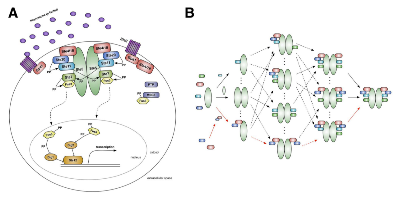
The pathway represents canonical mechanisms of the subcelluar signal propagation, such as G-protein activation via a GPCR, which is stimulated by pheromone ligands. The scaffold protein (Ste5) is recruited to the cell surface. Its major role is to insulate the kinase phosphorylation cascade from activating other related pathways. Ste5 dimerizes and aggregates five more proteins that phosphorylates each other forming an activation cascade. The last one is doubly activated mitogene-activated protein kinase (MAPK, Fus3) that travels to the nucleus and releases the transcription factor (TF) from its inhibitors. In this way TF transcribes genes regulating yeast mating behaviour.
The study is examining the established hypothesis that signals in cells are propagated via well defined complexes of molecular machines rather than loosely assembled and polymorphic ensembles.
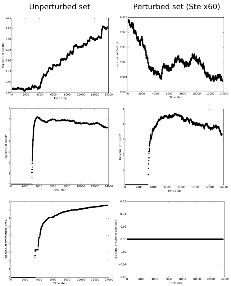
As it was shown, even though a conserved structure of decameric complex was hardly present in the ensemble model over repeated simulations, the signal was uninterrupted leading to St4 synthesis. Furthermore, contrary to the machine model, the ensemble model was able to replicate the experimental observation of combinatorial inhibition of phosphorylated Fuss3 (Fus3pp), when a copy-number of St5 was increased 60 fold. Models were built with the rule-based formalism that allows us to sample the sets of possible protein complexes the model can produce, without explicitly imposing the set of species that are formed [Suderman2013]. More details about the formalism are in the next section. The code with the models’ implementation is in the public domain and can be found as one of the attached files to this paper.
0.3 Rule-based modelling
The subject of signalling pathways and networks has already been addressed by many modelling formalisms. However, one significant advantage of the rule-based (RB) modelling is that it is able to express an infinite number of reactions with a small and finite number of rules, i.e. a single reaction rule and its parameters generalize a class of multiple interactions. In all of the other modelling methods every chemical species has to be specified in advance which is highly problematic for species with dozens of phosphorylation sites and many possible states. This limiting factor makes these methods inappropriate for modelling large-scale complex dynamical systems.
RB modelling is a method for the formal representation of combinatorially complex signalling systems in both a qualitative and quantitative way. The major idea is to replace equations with interaction rules. A rule representation is a graph-rewriting, where a graph specified on the left-hand-side is a pattern to be matched to instances in the current “mixture” of graphs and transformed into graphs specified on the right-hand-side. Matching should satisfy embedding, i.e. injections on agents (graphs) with the preservation of names, sites, internal states and edges [Danos2007]. In the rule-based language nomenclature, “agents” are most elementary molecules and “species” are agent complexes having particular states. A model can be translated into a system of ODE equations or simulated with a stochastic algorithm. In the latter case, system trajectories are created by rule selection at each time step, which is applied probabilistically, based on reaction rates and the initial/current copy number of agents [Hlavacek2006]. Immediate consequences of this formulation are different levels of rule contextualisation (“don’t care don’t write”), without obligation of ad hoc assumptions about the system, modularity, reusability and extensibility of the modelling process [Lopez2013]. Furthermore, the ability to capture a protein as a graph with (binding) sites (e.g. domains) that have internal state(s) (e.g. phosphorylated) gives a sufficiently expressive system to capture all of the principal mechanisms of signalling processes (e.g. dissociation, synthesis, degradation, binding, complex formation [Liu2012]) as well as insight into site-specific details of molecular interactions such as affinities, dynamics of post-translational modifications, domain availability, competitive binding, causality and the intrinsic structure of interactions.
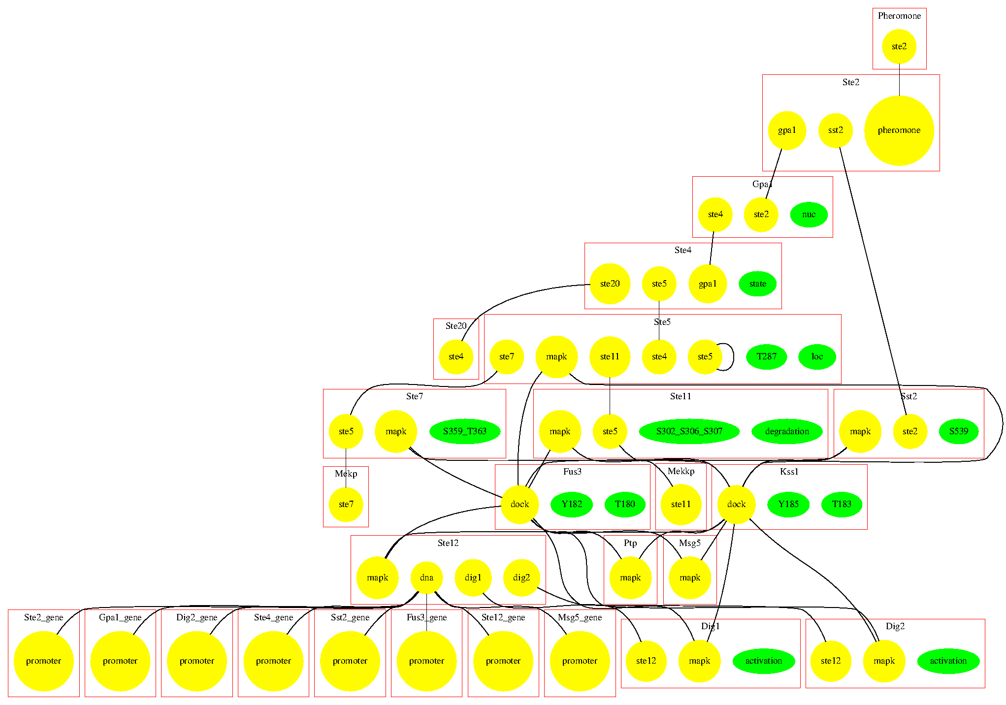
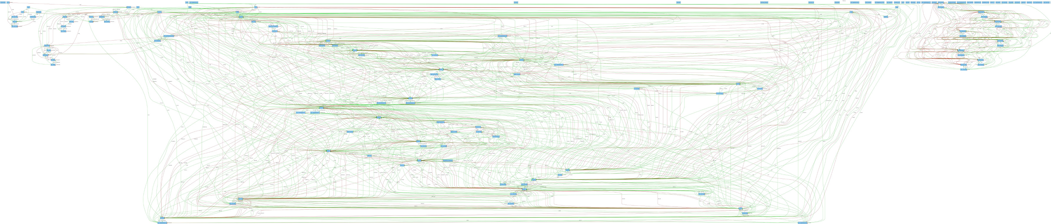
RB modelling originates from concurrency system representations and as such has the ability to capture dependencies, causality and conflicts in biological interactions (overlooked by concentration-based ODEs). In other words, precedences occurring along trajectories (stories) reveal competing events leading to a final state [Danos2007]. In the Kappa language, this feature is supported by the syntax for graphical analysis provided in the simulation tool. Among these are diagrams with causal flows, flux and influence maps as well as contact maps [Figure 2] that facilitate the process of modelling. The causal flow diagram shows dependencies and conflicts in tracking indicated species and the flux maps [Figure 3], negative/positive activity transfers between rules with the quantitative contributions on edge weights, both generated on the fly during a simulation [Feret2012]. At any time of a simulation, a snapshot can be taken to record the collection of species existing at that time.
0.4 Datasets and simulations
Our time series datasets report changes of indicated molecular species’ copy-number over 13,800 time points. Stochastic simulations were run for 4,600 sec with 3 time points recorded per second. The system was first simulated over 1,000 sec to reach a steady state and the initial mixture of protein complexes. Afterwords, a pheromone stimulus was introduced and the system was simulated for another 3,600 sec.
Variables in the rule-based syntax are called “observables” ( %obs:) and are specified in a separate code block. A single observable can be mapped to one or more rules conditioned on the level of its particularity. Hence, all the types of created species not indicated as observables, become intractable. For instance, the observable %obs: Fus3PPFus3(T180~p,Y182~p), which is a double phosphorylated MAPK kinase Fus3, is associated with 14 rules of the following form:
-
•
Fus3(dock!1,T180~p,Y182~p),Sst2(S539,mapk!1)
-> Fus3(dock,T180~p,Y182~p),Sst2(S539,mapk) -
•
Ste7(ste5!2,S359_T363~pp,mapk!1),Ste5(ste7!2), Fus3(dock!1,T180~p,Y182~p)
-> Ste7(ste5,S359_T363~pp,mapk),Ste5(ste7),
Fus3(dock,T180~p,Y182~p) -
•
Fus3(dock!1,T180~p,Y182~p),Ste11(mapk!1)
-> Fus3(dock,T180~p,Y182~p),Ste11(mapk) -
•
Ste5(ste7!1),Ste7(mapk!2,ste5!1,S359_T363~pp), Fus3(dock!2,T180~p,Y182~u)
-> Ste5(ste7!1),Ste7(mapk!2,ste5!1,S359_T363~pp),
Fus3(dock!2,T180~p,Y182~p) -
•
...etc.
However, as it is with the model specification, as it is infeasible to observe all potentially important variations of species, we have to resort to what we know we want to observe.
Therefore, the considered dataset consists of standard 31 variables, patterned after the original paper. There is also an extended 977 variable set but it has yet to be explored with parallel computations. This number was dictated by the snapshot of all existing species at the pick of the simulation (~1,000 sec after the stimulus appearance) used then as a list of observables in the simulation.
0.4.1 Perturbed model
To compare the outcome of applied methods, the model was simulated in two states, which are called here “perturbed” and “unperturbed”. By the unperturbed model we call the standard “wild type” pathway dynamics. The perturbed one relates to an experimentally observed phenomenon of combinatorial inhibition. It occurs when the copy-number of protein scaffold is largely increased and impossible to fully assemble the complex that doubly activates Fus3 because all available members of the complex are used up on too many scaffold proteins.
0.4.2 Simulator
Models written in Kappa language are supported by KaSim simulator. By default, reaction rates are computed applying the law of mass action [Chylek2014] but can easily be adjusted to follow any kinetic law (e.g. Michaelis-Menten, Hill’s Law). What can be found under the hood is a direct particle-based variant of Gillespie’s method. A general version of Gillespie’s method, also called exact stochastic simulation algorithm (SSA) or kinetic Monte Carlo is a common simulation method for modelling time-evolution of stochastic chemical reaction systems. Numerical stochastic simulations are known to be computationally intensive and a lot of efforts have been made to improve their efficiency [Gillespie2007]. The most popular and effective solution, implemented in KaSim, is called “network-free” because rules transforming reactant into products are applied directly at runtime to advance the state of a system. As a result, it does not have to generate the full reaction network beforehand and is therefore independent of its size [Hogg2014].