Sparse Grid Approximation Spaces for Space-Time Boundary Integral Formulations of the Heat Equation

Abstract

The aim of this paper is to develop stable and accurate numerical schemes for boundary integral formulations of the heat equation with Dirichlet boundary conditions. The accuracy of Galerkin discretisations for the resulting boundary integral formulations depends mainly on the choice of discretisation space. We develop a-priori error analysis utilising a proof technique that involves norm equivalences in hierarchical wavelet subspace decompositions. We apply this to a full tensor product discretisation, showing improvements over existing results, particularly for discretisation spaces having low polynomial degrees. We then use the norm equivalences to show that an anisotropic sparse grid discretisation yields even higher convergence rates. Finally, a simple adaptive scheme is proposed to suggest an optimal shape for the sparse grid index sets.

1 Introduction

Solutions to the heat equation are needed in many applications in physics, engineering and financial modeling [1], [2]. The primary application in three dimensions is modeling heat flow in an isotropic medium. Higher dimensional applications appear in, e.g. the valuation of financial derivatives or in image analysis and machine learning [3]. Since the analytic solutions to these problems are typically not known, efficient numerical methods for solving them are important.

Standard methods for solving parabolic boundary value problems, such as finite element methods, approximate the solution using a variational formulation on a subdivision of the domain $\Omega$ combined with a low-order time stepping scheme [4]. Efficient variants of this finite element approach using various space-time sparse grid discretisations can be found in e.g. [5]. In complicated spatial domains, or for unbounded domains, generating a mesh of the domain $\Omega$ can be extremely challenging. In contrast, the boundary integral formulation of the problem only requires a mesh of the boundary $\Gamma=\partial\Omega$. In many applications only the boundary values of the solution or its derivatives are the quantities of interest. This data can be obtained directly as a solution of the boundary integral formulation.

After the boundary reduction the resulting Galerkin boundary integral formulation of the heat equation becomes coercive [6]. Hence it remains stable for any conforming space-time discretisation. In particular, it remains stable for arbitrary choices of mesh size versus time step size. For problems with inhomogeneous stationary boundary conditions, this allows us to solve the equation much more efficiently, as a small number of time steps is sufficient. In order to allow easy error analysis of these methods for different choices of discrete approximation spaces we restrict ourselves to a Galerkin discretisation of the problem.

The main aim of this paper is to show that the boundary integral formulation provides a stable method to solve the heat equation for various choices of discretisation spaces. We will supplement the obtained theoretical bounds by numerical experiments. The computational gains of the boundary integral formulation are easily lost with a naive implementation of the method, largely due to the resultant full stiffness matrices and singular integrals. In a subsequent paper we will expand on how to resolve these implementational issues.

The paper is organised as follows. In Section 2 we formulate the heat equation, introduce the boundary reduction and the anisotropic Sobolev spaces that the boundary integral operators are posed in.

In Section 3 we will show that the classical convergence results from [6] can be improved for particular choices of polynomial degrees by using a wavelet decomposition of the discrete spaces. More precisely, this error analysis yields an improvement for low polynomial degrees. These low order polynomials are of interest as they can be easily implemented, even when using wavelet bases.

In Section 4 we improve on the error analysis of the sparse grid approximations to this problem given in [7] and [8] and verify those results numerically. We show that the combination technique ([9], [10]) gives an efficient and easily implemented approximation of the sparse grid space for this problem.

Further, we show examples of index sets produced by a simple adaptive algorithm. The adaptive implementation suggests that the approximation spaces constructed in [11] give higher convergence rates for these problems if an appropriate anisotropic scaling in time and space is chosen.

2 Problem Formulation

We start by formulating the domain heat equation. Let $\Omega\subset\mathbb{R}^{d}$, $d\geq 2$ be a bounded domain with a smooth boundary $\Gamma:=\partial\Omega$. The extension of the following theory to non-smooth, e.g. polygonal domains, is possible [12], [6]. However, for simplicity we restrict ourselves to smooth domains $\Gamma\subset C^{\infty}$. Further, let $n$ be the outer normal vector field of $\Gamma$.

With $T>0$ we denote a finite time horizon and with $\mathcal{I}:=(0,T)$ the time interval of interest. The domain heat equation is defined on the space-time cylinder $Q:=\Omega\times\mathcal{I}$.

Definition 2.1.

Given boundary data $g:\Gamma\times\mathcal{I}\rightarrow\mathbb{R}$ find the solution $u:Q\rightarrow\mathbb{R}$ satisfying:

$$\begin{split}(\partial_{t}-\Delta)u&=0,~{}~{}~{}~{}~{}~{}~{}~{}~{}~{}\text{in }Q\\ u&=0,~{}~{}~{}~{}~{}~{}~{}~{}~{}~{}\text{at }\Omega\times\{t=0\}\\ Tu&=g,~{}~{}~{}~{}~{}~{}~{}~{}~{}~{}\text{in }\Gamma\times\mathcal{I},\end{split}$$ (1)

where $T$ is the trace operator $\gamma_{0}u=u|_{\Gamma}$ in the case of Dirichlet boundary conditions, or the normal derivative of the solution on the boundary $\gamma_{1}u=\partial_{n}u|_{\Gamma}$ in the case of Neumann boundary conditions.

2.1 Boundary reduction

The boundary element method relies on finding a formulation of the problem (1) which is posed on the mantle of the space-time cylinder $\Omega\times\mathcal{I}$. For this we require the fundamental solution of the heat equation, which is

$$G(x,t)=\begin{cases}(4\pi t)^{-d/2}e^{-|x|^{2}/4t}&t\geq 0\\ 0&t<0,\end{cases}$$ (2)

for any spatial dimension $d\geq 1$ (see [6]).

Then we can apply Green’s second theorem to problem (1) with either Dirichlet or Neumann boundary conditions, giving the following representation of the solution of the heat equation

$$\begin{split}u(x,t)=\int_{0}^{T}\int_{\partial\Omega}&\left[G(x-y,t-s)\frac{\partial}{\partial n_{y}}u(y,s)-\frac{\partial}{\partial n_{y}}G(x-y,t-s)u(y,s)\right]dyds,\end{split}$$ (3)

where $n_{y}$ is outward unit normal to $\partial\Omega$ at the point $y$.

The boundary element method then consists of finding the missing boundary data in (3). That is, either the boundary flux $\gamma_{1}u$ for the Dirichlet problem or the boundary values $\gamma_{0}u$ for the Neumann problem. This formulation can be simplified using the following operators:

Definition 2.2.

The single layer heat potential is defined as

$$\mathcal{K}_{0}(\varphi)(x,t):=\int_{\Sigma}\varphi(y,s)G(x-y,t-s)dyds~{}~{}~{}~{}~{}~{}~{}~{}~{}(x,t)\in Q$$

The double layer heat potential is defined as

$$\mathcal{K}_{1}(\psi)(x,t):=\int_{\Sigma}\psi(y,s)\frac{\partial}{\partial n_{y}}G(x-y,t-s)dyds~{}~{}~{}~{}~{}~{}~{}~{}~{}(x,t)\in Q.$$

Using the trace operators $\gamma_{0}$ and $\gamma_{1}$, the representation formula (3) can now be written more concisely as

$$u=\mathcal{K}_{0}(\gamma_{1}u)-\mathcal{K}_{1}(\gamma_{0}u),~{}~{}~{}~{}~{}~{}\text{in Q}.$$ (4)

Let $\varphi\in H^{\frac{1}{2},\frac{1}{4}}(\Sigma)$ and $\psi\in H^{-\frac{1}{2},-\frac{1}{4}}(\Sigma)$.

Definition 2.3.

The single layer operator $V$ is defined as

$$V\psi:=\gamma_{0}\mathcal{K}_{0}\psi.$$ (5)

and the double layer operator $K$ is defined as

$$K\varphi:=\gamma_{0}\left(\mathcal{K}_{1}\varphi\right)|_{Q}+\frac{1}{2}\varphi.$$ (6)

An extensive analysis of these operators, including results on their well-posedness and regularity can be found in [6] and [12]. Using these operators we can formulate two methods to find solutions of the boundary integral formulation of the heat equation. For this we first need to introduce the anisotropic Sobolev spaces these methods are posed in. Let $r,s\geq 0$ then

$$\begin{split}H^{r,s}(\mathbb{R}^{d}\times\mathbb{R})&:=L^{2}(\mathbb{R};H^{r}(\mathbb{R}^{d}))\cap H^{s}(\mathbb{R};L^{2}(\mathbb{R}^{d})),\end{split}$$

Their dual spaces are given by $H^{-r,-s}:=(H^{r,s})^{\prime}$.

We restrict these spaces to the bounded domain $Q$:

$$\begin{split}H^{r,s}(Q)&:=\{u|_{Q}~{}:~{}u\in H^{r,s}(\mathbb{R}^{d}\times\mathbb{R})\},\\ H^{r,s}(\Sigma)&:=\{u|_{\Sigma}~{}:~{}u\in H^{r,s}(\mathbb{R}^{d}\times\mathbb{R})\}.\end{split}$$

They are equipped with the graph norm:

$$\begin{split}\|u\|_{H^{r,s}(Q)}&=\|u\|_{L^{2}(\mathcal{I};H^{r}(D))}+\|u\|_{H^{s}(\mathcal{I};L^{2}(D))}\\ &\sim\|u\|_{H^{r}(D)\otimes L^{2}(\mathcal{I})}+\|u\|_{L^{2}(D)\otimes H^{s}(\mathcal{I})}\end{split}$$

These spaces are well-defined for $(r,s)\in[-1,1]\times\mathbb{R}$ if $\Gamma\in C^{0,1}$ and for all $r,s\in\mathbb{R}$ if $\Gamma\in C^{\infty}$ [6].

The Sobolev spaces with zero initial conditions at $t=0$ will be denoted by

$$\begin{split}\tilde{H}^{r,s}(Q)&:=\{u|_{Q}~{}:~{}u\in H^{r,s}((-\infty,T)\times\Omega),~{}u(x,t)=0,~{}t<0\},\\ \tilde{H}^{r,s}(\Sigma)&:=\{u|_{\Sigma}~{}:~{}u\in H^{r,s}((-\infty,T)\times\Gamma),~{}u(x,t)=0,~{}t<0\}.\end{split}$$

For the sake of simplicity we will restrict ourselves in the following to Dirichlet boundary conditions $Tu=\gamma_{0}u$ and vanishing source terms $f=0$.

We are now ready to give the two formulations of the boundary element method we will work with. The direct method first calculates the boundary flux of the solution and then uses the representation formula to find the solution itself. This is particularly useful in engineering applications, where the boundary flux is itself a quantity of interest [6].

The direct method:

1. Find $\psi\in H^{-\frac{1}{2},-\frac{1}{4}}(\Sigma)$ such that:

   $$V\psi=\left(\frac{1}{2}I+K\right)g.$$ (7)

2. Then the unique solution $u\in\tilde{H}^{1,\frac{1}{2}}(Q)$ of the Dirichlet problem (1) with $f=0$ can be represented by

   $$u=\mathcal{K}_{0}\psi-\mathcal{K}_{1}g.$$ (8)

The second method we introduce is called the indirect method. The main advantage of this method is that only the single layer operator $V$ needs to be assembled. This method could be used if the boundary flux is of no particular interest since the intermediate solution $\psi$ has no particular physical meaning [6].

The indirect method:

1. Find $\psi\in H^{-\frac{1}{2},-\frac{1}{4}}(\Sigma)$ such that:

   $$V\psi=g.$$ (9)

2. Then the unique solution $u\in\tilde{H}^{1,\frac{1}{2}}(Q)$ of the Dirichlet problem (1) with $f=0$ can be represented by

   $$u=\mathcal{K}_{0}\psi.$$ (10)

2.2 Galerkin discretisation

We now discretise these operators in time and space. In the following sections we will discuss several different choices of discrete spaces, so we initially keep the notation of this section general. Let $\mathcal{X}_{L}$ be a nested sequence of discrete spaces dense in $H^{-\frac{1}{2},-\frac{1}{4}}(\Sigma)$, i.e.

$$\mathcal{X}_{0}\subset\mathcal{X}_{1}\subset...\subset\mathcal{X}_{L}\subset...\subset H^{-\frac{1}{2},-\frac{1}{4}}(\Sigma).$$

Then, the direct and indirect formulations of the heat equation with Dirichlet data in the variational form are:

$$\begin{split}&\text{Find }\psi_{L}\in\mathcal{X}_{L}\text{ such that}\\ &~{}~{}~{}~{}~{}~{}~{}\langle V\psi_{L},\eta\rangle=\langle g,\eta\rangle,~{}~{}~{}~{}\,~{}~{}~{}~{}~{}~{}~{}~{}~{}\text{for all }\eta\in\mathcal{X}_{L}~{}~{}\text{ (Indirect method)}\\ &\text{or }~{}~{}~{}\langle V\psi_{L},\eta\rangle=\langle(\frac{1}{2}+K)g,\eta\rangle,~{}~{}~{}\text{for all }\eta\in\mathcal{X}_{L}~{}~{}\text{ (Direct method)}\end{split}$$ (11)

The following lemma follows directly from the Lax-Milgram Lemma and the Lemma of Céa respectively, using the coercivity and continuity of $V$ in the appropriate anisotropic Sobolev spaces described above. See [6] for further details.

Lemma 2.4.

The solution $\psi_{L}\in\mathcal{X}_{L}$ of the problems (11) is unique and quasi-optimal:

$$\|\psi-\psi_{L}\|_{H^{-\frac{1}{2},-\frac{1}{4}}(\Sigma)}\leq\frac{\|V\|}{c_{v}}\underset{\eta_{L}\in\mathcal{X}_{L}}{\inf}\|\psi-\eta_{L}\|_{H^{-\frac{1}{2},-\frac{1}{4}}(\Sigma)}.$$ (12)

Here $\|V\|$ and $c_{v}$ are the continuity and coercivity constants of the single layer heat operator $V$ respectively.

Let $\{b_{i}(x,t)\}_{i=1...N}=\{b_{i_{x}}(x)\cdot b_{i_{t}}(t)\}_{i=(i_{x},i_{t})}$ be a basis of the discrete space $\mathcal{X}_{L}$, where $N$ is the number of basis functions. Then, finding the discrete solution $\psi=\sum_{j=1}^{N}c_{j}b_{j}\in\mathcal{X}_{L}$ requires the solution of a linear system of the form

$$\sum_{j=1}^{N}\langle Vb_{j},b_{i}\rangle c_{j}=\langle g,b_{i}\rangle,~{}~{}~{}~{}\forall i={1...N}.$$

We refer to the resultant matrix as $A_{i,j}=\langle Vb_{j},b_{i}\rangle$. The structure of the matrix $A$ follows directly from the form of the fundamental solution. In particular, since $G(x,t)=0$ if $t<0$, the matrix is block lower triangular.

3 Error Analysis for Full Tensor-products

We start with a simple discretisation of the integral formulation of the heat equation using tensor products of piecewise polynomial basis functions in time and space. In this section we give improved error bounds for certain choices of polynomial degrees. The classical theory due to [6] uses an Aubin-Nitsche duality argument and properties of the $L^{2}$-orthogonal projection. We propose a new proof using as a main ingredient norm equivalences, which can be shown using a wavelet decomposition of the discrete spaces.

We start by introducing the spaces of piecewise polynomials in time and space. Let $\mathcal{X}_{i}^{x}$ and $\mathcal{X}_{j}^{t}$ be the nested finite element spaces:

$$\begin{split}&\mathcal{X}_{0}^{x}\subset\mathcal{X}_{1}^{x}\subset....\subset\mathcal{X}^{x}_{i}\subset H^{-\frac{1}{2}}(\Gamma)\text{ and }\\ &\mathcal{X}_{0}^{t}\subset\mathcal{X}_{1}^{t}\subset....\subset\mathcal{X}^{t}_{j}\subset H^{-\frac{1}{4}}(\mathcal{I}).\end{split}$$

In time we simply define the discrete spaces as discontinuous piecewise polynomials on an equidistant grid, which is refined by bisection. More precisely,

$$\mathcal{X}_{j}^{t}=\{v\in L^{2}(\mathcal{I})~{}:~{}v|_{[t_{k},t_{k+1}]}\in\mathcal{P}_{p_{t}},~{}p_{t}\geq 0,~{}k=0,\dots,2^{j}-1\}.$$

In space we define the discrete spaces using parameterisations $\gamma:[0,1]^{d-1}\rightarrow\Gamma$ of the boundary of the spatial domain. In two dimensions the smooth boundary $\Gamma$ can be paramaterised using a single smooth, $1$-periodic function $\gamma$. In higher dimensions or in the case of a piecewise smooth boundary $\Gamma$ the domain is cut up into non-overlapping patches and each is parameterised by a smooth function. Thus,

$$\mathcal{X}_{i}^{x}=\{v\in L^{2}(\Gamma)~{}:~{}v|_{\tau}\circ\gamma\in\mathcal{P}_{p_{x}},~{}p_{x}\geq 0~{}\forall\tau\in\tau_{i}\},$$

where $\tau_{i}$ is the triangulation of the boundary at level $i$ and $\mathcal{P}_{p_{x}}$ is the space of polynomials of degree $p_{x}$. Again, we refine by halving the support of the basis functions in each direction. For a two dimensional problem this is simply a bisection. For a three dimensional problem discretised using triangles this corresponds to a red refinement.

Then the full tensor product space $\mathcal{X}_{L}$ can be defined as

$$\mathcal{X}_{L}=\mathcal{X}_{L}^{x}\oplus\mathcal{X}_{L}^{t}.$$

Next we introduce a multilevel decomposition of the space $\mathcal{X}_{L}$. This decomposition is needed to show the norm equivalences that are central to the proof. We construct a system of subspaces $W_{j}$, that are pairwise orthogonal with respect to the $L^{2}$ inner product. They give a multilevel decomposition of $\mathcal{X}^{x}_{i}$ as follows:

$$\mathcal{X}^{x}_{i}=W^{x}_{0}\oplus...\oplus W^{x}_{i},~{}~{}~{}~{}~{}\mathcal{X}^{t}_{j}=W^{t}_{0}\oplus...\oplus W^{t}_{j}$$ (13)

In particular, for $\psi\in H^{r,s}(\Sigma)$ with $\psi=\sum_{(\ell_{x},\ell_{t})\geq 0}w_{(\ell_{x},\ell_{t})}$ and $w_{(i,j)}\in W_{i}^{x}\otimes W_{j}^{t}$, we have (see [11])

$$\|\psi\|_{H^{r,s}(\Sigma)}^{2}\sim\left\{\begin{array}[]{cl}\sum_{(\ell_{x},\ell_{t})\geq 0}2^{2\max\{r\ell_{x},s\ell_{t}\}}\|w_{(\ell_{x},\ell_{t})}\|^{2}_{L^{2}(\Sigma)},&r,s\geq 0,\\[6.45831pt] \sum_{(\ell_{x},\ell_{t})\geq 0}2^{-2\max\{|r|l_{x},|s|l_{t}\}}\|w_{(\ell_{x},\ell_{t})}\|^{2}_{L^{2}(\Sigma)},&r,s<0.\end{array}\right.$$ (14)

These norm equivalences deliver (sharp) upper and lower bounds for the error estimates, which we use in the forthcoming error analysis.

We generalise the tensor product spaces of the form $\mathcal{X}_{L}^{x}\otimes\mathcal{X}^{t}_{L}$ by using the above multilevel decomposition and including $W^{x}_{i}\otimes W^{t}_{j}$ for certain indices $(i,j)$. The resulting spaces are then described fully by the indices of the included subspaces. The index set corresponding to the anisotropic full tensor product space is

$$I_{L}^{\sigma}=\{(\ell_{x},\ell_{t})~{}:~{}\ell_{x}\leq L/\sigma,~{}\ell_{t}\leq\sigma L\},$$ (15)

where $\sigma$ is a positive real parameter that can be chosen freely. The form of scaling used here mirrors the definition of anisotropic sparse grid index sets from [13] and allows us to easily compare to those sets in Section 4. The index set is visualised in Figure 1. In subsequent sections we will characterise various sparse grid discretisation spaces by other choices of index set.

The parameter $\sigma$ denotes the scaling in time and space. For example, if $\sigma=2$, we use four times as many discretisation levels in time than in space. On the other hand if $\sigma<1$ we refine more strongly in space than in time.

Recall that $\psi=\sum_{(\ell_{x},\ell_{t})\geq 0}w_{(\ell_{x},\ell_{t})}$. Then by letting $\psi_{L}=\sum_{(\ell_{x},\ell_{t})\in I_{L}^{\sigma}}w_{(\ell_{x},\ell_{t})}\in\mathcal{X}_{L}$ we get the following by applying (14) twice.

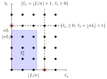
Figure 1: The full tensor product index set $I_{L}^{\sigma}$. The two potential minima outside the set $I_{L}^{\sigma}$ are circled in red.

$$\begin{split}&\inf_{\psi_{L}\in\mathcal{X}_{L}}\|\psi-\psi_{L}\|^{2}_{H^{-\frac{1}{2},-\frac{1}{4}}(\Sigma)}\sim\sum_{(\ell_{x},\ell_{t})\notin I_{L}^{\sigma}}2^{-2\max\{\frac{\ell_{x}}{2},\frac{\ell_{t}}{4}\}}\|w_{(\ell_{x},\ell_{t})}\|^{2}_{L^{2}(\Sigma)}\\ &\leq\left(\max_{(\ell_{x},\ell_{t})\notin I_{L}^{\sigma}}2^{-2\max\{\frac{\ell_{x}}{2},\frac{\ell_{t}}{4}\}-2\max\{\mu\ell_{x},\lambda\ell_{t}\}}\right)\cdot\sum_{(\ell_{x},\ell_{t})\notin I_{L}^{\sigma}}2^{2\max\{\mu\ell_{x},\lambda\ell_{t}\}}\|w_{(\ell_{x},\ell_{t})}\|^{2}_{L^{2}(\Sigma)}\\ &\leq\left(\max_{(\ell_{x},\ell_{t})\notin I_{L}^{\sigma}}2^{-2\max\{\frac{\ell_{x}}{2},\frac{\ell_{t}}{4}\}-2\max\{\mu\ell_{x},\lambda\ell_{t}\}}\right)\cdot\|\psi\|^{2}_{H^{\mu,\lambda}(\Sigma)}.\end{split}$$ (16)

The term $2^{-2(\max\{\frac{\ell_{x}}{2},\frac{\ell_{t}}{4}\}+2\max\{\mu\ell_{x},\lambda\ell_{t}\})}$ reaches its maximum when the negative exponent is as small as possible. We define

$$f(\ell_{x},\ell_{t}):=\max\left\{\frac{\ell_{x}}{2},\frac{\ell_{t}}{4}\right\}+\max\{\mu\ell_{x},\lambda\ell_{t}\}.$$ (17)

Then, in order to determine the error bound we find the minimum

$$n:=\min_{(\ell_{x},\ell_{t})\notin I_{L}^{\sigma}}f(\ell_{x},\ell_{t}).$$ (18)

To do so we use the following properties of monotonically increasing functions.

Definition 3.5.

The function $F(\ell_{x},\ell_{t})$ is called a monotonically increasing function if

$$\begin{split}&F(\ell_{x}+k,\ell_{t})\geq F(\ell_{x},\ell_{t}),~{}~{}~{}~{}~{}~{}\forall k\geq 0\quad\text{ and }\\ &F(\ell_{x},\ell_{t}+k)\geq F(\ell_{x},\ell_{t}),~{}~{}~{}~{}~{}~{}\forall k\geq 0.\end{split}$$

Lemma 3.6.

Let $F$ be a monotonically increasing function. Then its minimum outside the set $I_{L}^{\sigma}$ is

$$\min_{(\ell_{x},\ell_{t})\notin I_{L}^{\sigma}}F(\ell_{x},\ell_{t})=\min\{F(\lfloor L/\sigma\rfloor+1,0),F(0,\left\lfloor\sigma L\right\rfloor+1)\}.$$

Proof.

Let $\ell_{x}\geq L/\sigma+1$ Then there holds

$$F(\ell_{x},\ell_{t})\geq F(\lfloor L/\sigma\rfloor+1,\ell_{t})$$

by Definition 3.5. Analogously if we let $\ell_{t}\geq\left\lfloor\sigma L\right\rfloor+1$, there holds

$$F(\ell_{x},\ell_{t})\geq F(\ell_{x},\left\lfloor\sigma L\right\rfloor+1)$$

Together this tells us that the minimising multi-index lies in the subset

$$\{(\ell_{x},\ell_{t})~{}:~{}\ell_{x}=\lfloor L/\sigma\rfloor+1\text{ or }l_{t}=\left\lfloor\sigma L\right\rfloor+1\}\subset\{(\ell_{x},\ell_{t})\notin I_{L}^{\sigma}\}.$$

In Figure 1 this subset is depicted by the dashed lines.

Now let $\ell_{x}=\lfloor L/\sigma\rfloor+1$ and $\ell_{t}\geq 0$, then there holds

$$F(\ell_{x},\ell_{t})\geq F(\lfloor L/\sigma\rfloor+1,0).$$

Analogously, for $\ell_{x}\geq 0$ and $\ell_{t}=\left\lfloor\sigma L\right\rfloor+1$ we have

$$F(\ell_{x},\ell_{t})\geq F(0,\left\lfloor\sigma L\right\rfloor+1).$$

This shows that the minimum can only be attained at $(\lfloor L/\sigma\rfloor+1,0)$ or $(0,\left\lfloor\sigma L\right\rfloor+1)$ as asserted. ∎

To estimate the convergence rate from (16) we require the minimum $n$ defined in (18). Clearly, the function of the exponent $f(\ell_{x},\ell_{t})$ is a monotonically increasing function. Using Lemma 3.6 we get

$$\begin{split}n&=\min_{(\ell_{x},\ell_{t})\notin I_{L}^{\sigma}}f(\ell_{x},\ell_{t})=\min\left\{\left(\mu+\frac{1}{2}\right)\left(\lfloor L/\sigma\rfloor+1\right),\left(\lambda+\frac{1}{4}\right)\left(\left\lfloor\sigma L\right\rfloor+1\right)\right\}\\ &\sim\min\left\{\left(\mu+\frac{1}{2}\right)\sigma^{-1},\left(\lambda+\frac{1}{4}\right)\sigma\right\}(L+1).\end{split}$$

Thus, the minimum is

$$n\sim(L+1)\begin{cases}\left(\lambda+\dfrac{1}{4}\right)\sigma,&\sigma^{2}\leq\dfrac{\mu+1/2}{\lambda+1/4}\\[8.61108pt] \left(\mu+\dfrac{1}{2}\right)\sigma^{-1},&\text{else}.\end{cases}$$ (19)

We can now formulate the following theorem on the convergence in the energy norm.

Theorem 3.7.

Let $d>1$ and let $\mu,\lambda$ fulfil $\mu\leq p_{x}+1$ and $\lambda\leq p_{t}+1$ and let $c>0$ be a constant depending only on $\sigma,d,\mu$ and $\lambda$. Further, denote by $N_{L}$ the total number of degrees of freedom, i.e. $N_{L}\sim 2^{(\sigma+(d-1)/\sigma)L}$. Then the convergence in the energy norm is

$$\|\psi-\psi_{L}\|_{H^{-\frac{1}{2},-\frac{1}{4}}(\Sigma)}^{2}\leq cN_{L}^{-\frac{2\mu+1}{d-1+\sigma^{2}}}\|\psi\|_{H^{\mu,\lambda}(\Sigma)}^{2}\quad\text{for}\quad\sigma^{2}=\frac{\mu+1/2}{\lambda+1/4}.$$

Proof.

Inserting the exponent $n$ from (19) into (16) we get

$$\|\psi-\psi_{L}\|_{H^{-\frac{1}{2},-\frac{1}{4}}(\Sigma)}^{2}\leq c2^{-2n}\|\psi\|_{H^{\mu,\lambda}(\Sigma)}^{2}$$

For $\sigma^{2}=\frac{\mu+1/2}{\lambda+1/4}$ we have $n=\left(\lambda+\dfrac{1}{4}\right)\sigma=\left(\mu+\dfrac{1}{2}\right)\sigma^{-1}$. Finally, rewriting in terms of degrees of freedom $N_{L}\sim 2^{(\sigma+(d-1)/\sigma)L}$ we get

$$\begin{split}\|\psi-\psi_{L}\|_{H^{-\frac{1}{2},-\frac{1}{4}}(\Sigma)}^{2}&\leq cN_{L}^{-\frac{2\mu+1}{d-1+\sigma^{2}}}\|\psi\|_{H^{\mu,\lambda}(\Sigma)}^{2}.\end{split}$$

∎

Remark 1.

The highest possible rate of convergence is attained in the space $H^{p_{x}+1,p_{t}+1}(\Sigma)$, so we restrict the regularity constants $\mu$ and $\lambda$ by the polynomial degrees $p_{x}+1$ and $p_{t}+1$ respectively [13].

Full tensor product, $d=2$
$(p_{x},p_{t})$	conv. rate $\gamma$	scaling $\sigma^{2}$
$(0,0)$	$\frac{15}{22}\sim.7$	$\frac{6}{5}$
$(1,0)$	$\frac{5}{6}\sim.8$	$2$
$(0,1)$	$\frac{9}{10}\sim.9$	$\frac{2}{3}$
$(1,1)$	$\frac{45}{38}\sim 1.2$	$\frac{10}{9}$

Full tensor product, $d=3$
$(p_{x},p_{t})$	conv. rate $\gamma$	scaling $\sigma^{2}$
$(0,0)$	$\frac{15}{32}\sim.46$	$\frac{6}{5}$
$(1,0)$	$\frac{5}{8}\sim.62$	$2$
$(0,1)$	$\frac{9}{16}\sim.56$	$\frac{2}{3}$
$(1,1)$	$\frac{45}{56}\sim.8$	$\frac{10}{9}$

Table 1: Improved convergence rates and optimal values of $\sigma$ for full product discretisations in $2$ and $3$ dimensions.

In Table 1 we give the convergence rates and optimal choices of $\sigma$ for different combinations of polynomial degrees. In the case of an analytic solution the only constraints on $\mu$ and $\lambda$ lie in the polynomial degree of the discretisation. Thus, we can choose $\mu=p_{x}+1$ and $\lambda=p_{t}+1$ to maximise the convergence rate. Then, the optimal scaling $\sigma$ can be written in terms of polynomial degree as $\sigma^{2}=\frac{4p_{x}+6}{4p_{t}+5}$. In two dimensions and for $p_{x}=p_{t}=0$ the optimal scaling is $\sigma=\frac{6}{5}$ and this gives a higher convergence rate than that for $\sigma=1$ in the classical theory from [6], suggesting that this scaling should be used instead.

As the polynomial degrees in time and space $p_{x}=p_{t}$ increase the improvement becomes smaller. The results from Theorem 3.7 and Table 1 give the largest improvement for the case $p_{x}=p_{t}=0$. This happens since for large $p_{x}=p_{t}$ the term $\frac{4\mu+2}{4\mu+1}$ approaches $1$ and thus the results approach the results given in [6].

3.1 Numerical Experiments

We now verify the expected convergence rates for different choices of scaling factor $\sigma^{2}$. In these numerical experiments we set the time horizon to $T=4$, giving the time interval $\mathcal{I}:=(0,4)$. We initially choose a unit circle $B_{1}(0)$ as the domain $\Omega$. Thus, $Q:=B_{1}(0)\times\mathcal{I}$ is the space-time cylinder with mantle $\Sigma=\partial B_{1}(0)\times\mathcal{I}$ and we solve the Dirichlet problem (1) with the right hand side $g(r,\varphi,t)=t^{2}\cos(\varphi)$. The advantage of this test is that the exact solution can be calculated to verify the numerical solution [14].

In Figure 2 we plot the convergence of the boundary flux in the energy norm squared. For the curve corresponding to the scaling $\sigma=6/5$ the expected convergence rate from Theorem 3.7 is $\frac{15}{11}$. As we can see the convergence rate is close to the predicated rate. We also run tests with two other values of $\sigma$. When $\sigma=1$, we have a slightly lower convergence rate, as predicted by (19). Further, the constant for $h_{t}\sim h_{x}^{6/5}$ leads to a lower overall error. The convergence rate in this case is expected to be $\frac{5}{4}$. Lastly, when $\sigma=2$ we expect a slower convergence rate of $1$ from (19). The numerical tests confirm these rates.

Next we give some more challenging tests on an ellipse with the semi-axes $a=0.8$ and $b=0.5$. For these tests it is simpler to use the indirect method, as the exact solution is not known. We use a value calculated with $\sim 3.3\cdot 10^{7}$ degrees of freedom as an approximation of the exact solution to calculate the error. For this test we use the more oscillatory right hand side $g(\varphi,t)=t^{2}\cos(2\varphi)$.

In Figure 3 one can see that the correspondence to the expected rates is good for $\sigma=2$, where we again expect a rate of exactly $1$. At $\sigma=1$ the rate should be $5/4=1.25$, and is in fact somewhat higher than that. In particular, the error for $\sigma=1$ is smaller than the error for $\sigma=\frac{6}{5}$. The reason for this discrepancy is not clear. The expected convergence rate for $\sigma=\frac{6}{5}$ is $\frac{15}{11}$, and Figure 3 shows a good correspondence to this rate.

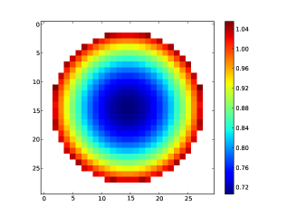
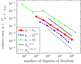
Figure 2: Convergence of the boundary flux in the energy norm for the right hand side $g(r,\varphi,t)=t^{2}\cos(\varphi)$ in the case $p_{x}=p_{t}=0$.

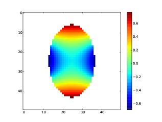
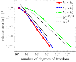
Figure 3: Left: The approximated solution on an ellipse for $g(\varphi,t)=t^{2}\cos(2\varphi)$ at timestep $t=1$. Right: Convergence of the boundary flux in squares of the energy norm for the right hand side $g(\varphi,t)=t^{2}\cos(2\varphi)$ on an ellipse with eccentricities $a=0.8,b=0.5$.

4 Sparse Grids

The natural tensor product structure of $\Sigma=\Gamma\times\mathcal{I}$ in space and time lends itself to a sparse grid approximation. The main idea behind these methods is to truncate the tensor-product expansion of a one-dimensional multilevel basis to improve the cardinality of the tensor product in space-time. To approximate a function such as $f(x,t)=f_{1}(x)f_{2}(t)$ that can be decomposed entirely in time and space the subspaces that are highly refined both in space and time can be dropped entirely without a loss of approximation properties. This is particularly helpful as these are precisely the most ’expensive’ subspaces, i.e. those containing the most degrees of freedom.

A sparse Galerkin discretisations yields only a mild dependence on the dimension. More precisely, standard sparse grid methods scale in dimension with $\mathcal{O}(N(\log N)^{d-1})$ [15], while the full tensor product scales with $\mathcal{O}(N^{d})$, where $N$ is the number of degrees of freedom. Thus, the sparse grid approximation can alleviate the ’curse of dimensionality’.

Let $\mathcal{X}_{L}^{x}$ be the discrete space in the spatial dimensions and $\mathcal{X}_{L}^{t}$ the discrete space in time. The first step in defining sparse grid structures is the definition of one-dimensional multilevel decompositions. They can then be combined to form sparse grid spaces. As in (13) assume that there exists a system of subspaces $W_{i}^{x}$ and $W_{j}^{t}$ such that

$$\mathcal{X}_{L}^{x}=W_{0}^{x}\oplus\cdots\oplus W_{L}^{x},\qquad\mathcal{X}_{L}^{t}=W_{0}^{t}\oplus\cdots\oplus W_{L}^{t}.$$

The general form of a sparse grid space in two dimensions is

$$\hat{\mathcal{X}}_{L}:=\bigotimes_{(\ell_{x},\ell_{t})\in J_{L}}W_{\ell_{x}}^{x}\otimes W_{\ell_{t}}^{t}\subset\mathcal{X}=H^{-\frac{1}{2},-\frac{1}{4}}(\Sigma)$$

where $J_{L}$ is an index set, which can be freely chosen.

The approximation properties of the space $\hat{\mathcal{X}}_{L}$ are entirely dependent on the choice of index set $J_{L}$. In Section 3 for example we have seen the approximation properties for the set index set $I_{L}^{\sigma}=\{(\ell_{x},\ell_{t})~{}:~{}\ell_{x}\leq L/\sigma,~{}\ell_{t}\leq\sigma L\}$, there we essentially only had to find the minimum of a monotonically increasing function outside of the subset $I_{L}$ in order to find the error in the energy norm. The same is true for more general index sets $J_{L}$.

Definition 4.8.

The standard anisotropic sparse grid index set is defined as

$$\hat{J}_{L}^{\sigma}=\left\{(\ell_{x},\ell_{t})~{}:~{}\ell_{x}\sigma+\ell_{t}/\sigma\leq L\right\},$$ (20)

where $0<\sigma<\infty$ is a free parameter (see e.g. [16]). In this case we write $\hat{\mathcal{X}}_{L}=\hat{\mathcal{X}}_{L}^{\sigma}$.

4.1 Error Analysis of Sparse Grids

An extensive error analysis of the standard sparse grid approximation to this problem has been shown in [7] and [8] using an Aubin-Nitsche based argument. As in the error analysis for the full tensor product spaces in Section 3 the main ingredient will be norm equivalences, shown using wavelet bases. For sparse grid approximation spaces the appropriate Sobolev spaces are spaces of weak mixed derivatives,

$$H^{r,s}_{\text{mix}}(\Sigma):=H^{r}(\Gamma)\otimes H^{s}(\mathcal{I}).$$ (21)

For $u\in H_{\text{mix}}^{r,s}(\Sigma)$ with $u=\sum_{(\ell_{x},\ell_{t})\geq 0}w_{(\ell_{x},\ell_{t})}$ and $w_{(\ell_{x},\ell_{t})}\in W_{\ell_{x}}\otimes W_{\ell_{t}}$, we have

$$\|u\|_{H^{r,s}_{\text{mix}}(\Sigma)}^{2}\sim\sum_{\ell_{x},\ell_{t}}2^{2(r\ell_{x}+s\ell_{t})}\|w_{(\ell_{x},\ell_{t})}\|^{2}_{L^{2}(\Sigma)}.$$ (22)

Define the set of indices outside of the sparse grid index set $\hat{J}_{L}^{\sigma}$ as

$$I=\{(\ell_{x},\ell_{t})~{}:~{}\ell_{x}\sigma+\ell_{t}/\sigma>L\}.$$

Then as in Section 3 we use the norm equivalences (22) to estimate

$$\begin{split}\|\psi-\psi_{L}\|_{H^{-\frac{1}{2},-\frac{1}{4}}(\Sigma)}^{2}\leq\sum_{(\ell_{x},\ell_{t})\notin J_{L}^{\sigma}}2^{-2\max\{\frac{\ell_{x}}{2},\frac{\ell_{t}}{4}\}-2(\mu\ell_{x}+\lambda\ell_{t})}\|\psi\|^{2}_{H^{\mu,\lambda}_{\text{mix}}(\Sigma)}.\end{split}$$

According to [13] the index set $I$ can be split into two disjoint sets $I=I_{1}\cup I_{2}$, given by

$$\begin{split}&I_{1}=\{(\ell_{x},\ell_{t})~{}:~{}0\leq\ell_{x}\leq\frac{L}{\sigma},~{}L\sigma-\ell_{x}\sigma^{2}<\ell_{t}\}\\ \text{and }&I_{2}=\{(\ell_{x},\ell_{t})~{}:~{}\frac{L}{\sigma}<\ell_{x},~{}0\leq\ell_{t}\}.\end{split}$$ (23)

We set $\tilde{f}(\ell_{x},\ell_{t}):=\max\{\frac{\ell_{x}}{2},\frac{\ell_{t}}{4}\}+(\mu\ell_{x}+\lambda\ell_{t})$ and apply the splitting (LABEL:eq-splitting) to estimate

$$\begin{split}\|\psi-\psi_{L}\|_{H^{-\frac{1}{2},-\frac{1}{4}}(\Sigma)}^{2}&\leq\sum_{(\ell_{x},\ell_{t})\in I}2^{-2\tilde{f}(\ell_{x},\ell_{t})}\|\psi\|^{2}_{H^{\mu,\lambda}_{\text{mix}}(\Sigma)}\\ &=\left(\sum_{\ell_{x}=0}^{\lfloor L/\sigma\rfloor}\sum_{\ell_{t}=\lfloor L\sigma-\ell_{x}\sigma^{2}\rfloor+1}^{\infty}2^{-2\tilde{f}(\ell_{x},\ell_{t})}+\sum_{\ell_{x}=\lfloor L/\sigma\rfloor+1}^{\infty}\sum_{\ell_{t}=0}^{\infty}2^{-2\tilde{f}(\ell_{x},\ell_{t})}\right)\|\psi\|^{2}_{H^{\mu,\lambda}_{\text{mix}}(\Sigma)}\end{split}$$

The terms of the infinite sums can be rewritten using the following well-known property of the geometric series $\sum_{k=m}^{\infty}r^{k}=\frac{r^{m}}{1-r},~{}r<1$. This gives

$$\begin{split}\|\psi-\psi_{L}\|_{H^{-\frac{1}{2},-\frac{1}{4}}(\Sigma)}^{2}&\lesssim\Big{(}\sum_{\ell_{x}=0}^{\lfloor L/\sigma\rfloor}2^{-2\tilde{f}(\ell_{x},\lfloor L\sigma-\ell_{x}\sigma^{2}\rfloor)}+\underbrace{2^{-2\tilde{f}(\lfloor L/\sigma\rfloor,0)}}_{\leq 2^{-2(\mu+\frac{1}{2})\lfloor L/\sigma\rfloor}}\Big{)}\|\psi\|^{2}_{H^{\mu,\lambda}_{\text{mix}}(\Sigma)}\end{split}$$

To estimate the first summand the exponent $\tilde{f}(\ell_{x},\lfloor L\sigma-\sigma^{2}\ell_{x}\rfloor)$ must be minimised in the range $0\leq\ell_{x}\leq\lfloor L/\sigma\rfloor$. This exponent is piecewise linear. Thus, its minima lie either at the limits of the range $\ell_{x}=0$ and $\ell_{x}=\lfloor L/\sigma\rfloor$ or at the turning point of $\tilde{f}(\ell_{x},\lfloor L\sigma-\sigma^{2}\ell_{x}\rfloor).$

Let $c>0$ be a constant that depends only on $\mu$ and $\lambda$. To simplify the expression and to determine the turning point we use the estimate $m-1\leq\lfloor m\rfloor$ and get

$$2^{-2\tilde{f}(\ell_{x},\lfloor L\sigma-\sigma^{2}\ell_{x}\rfloor)}\leq 2^{2(\lambda+\frac{1}{4})}2^{-2\tilde{f}(\ell_{x},L\sigma-\sigma^{2}\ell_{x})}\leq c2^{-2\tilde{f}(\ell_{x},L\sigma-\sigma^{2}\ell_{x})}.$$

Then the turning point of $\tilde{f}(\ell_{x},L\sigma-\sigma^{2}\ell_{x})$ lies at

$$\ell_{x}=\frac{L\sigma-\sigma^{2}\ell_{x}}{2}\Leftrightarrow\ell_{x}=\frac{L\sigma}{2+\sigma^{2}}.$$

We examine these three potential minima separately:

• $\ell_{x}=0,\,\ell_{t}=\lfloor L\sigma\rfloor$ gives the exponent: $\tilde{f}(0,\lfloor L\sigma\rfloor)=(\lambda+\frac{1}{4})\lfloor L\sigma\rfloor$. In this case we can estimate

  $$2^{-2\tilde{f}(0,\lfloor L\sigma\rfloor)}=2^{-2(\lambda+\frac{1}{4})\lfloor L\sigma\rfloor}\leq c2^{-2(\lambda+\frac{1}{4})L\sigma}.$$

• $\ell_{x}=\lfloor L/\sigma\rfloor,\ell_{t}=0$ gives the exponent $\tilde{f}(\lfloor L/\sigma\rfloor,0)(\mu+\frac{1}{2})\lfloor L/\sigma\rfloor$. In this case we can estimate

  $$2^{-2\tilde{f}(\lfloor L/\sigma\rfloor,0)}=2^{-2(\mu+\frac{1}{2})\lfloor L/\sigma\rfloor}\leq c2^{-2(\mu+\frac{1}{2})L/\sigma}.$$

• $\ell_{x}=\frac{L\sigma}{2+\sigma^{2}},\,\ell_{t}=2\ell_{x}$ gives the exponent $\tilde{f}(\ell_{x},2\ell_{x})=\left(\mu+2\lambda+\frac{1}{2}\right)L\frac{\sigma}{2+\sigma^{2}}$.

Taking these terms together we get

$$\|\psi-\psi_{L}\|_{H^{-\frac{1}{2},-\frac{1}{4}}(\Sigma)}^{2}\leq c2^{-2L\min\left\{\left(\mu+\frac{1}{2}\right)\sigma^{-1},\left(\lambda+\frac{1}{4}\right)\sigma,\left(2\lambda+\mu+\frac{1}{2}\right)\left(\frac{\sigma}{2+\sigma^{2}}\right)\right\}}\|\psi\|_{H^{\mu,\lambda}_{\text{mix}}(\Sigma)}.$$ (24)

Finally, we note that the dimension of the approximation space is given by (see [13]):

$$\dim(\hat{\mathcal{X}}_{L}^{\sigma})=:N_{L}\sim\begin{cases}2^{L\sigma}L,&\text{ if }\sigma^{2}=d-1,\\ 2^{L\max\{(d-1)/\sigma,\sigma\}},&\text{ else.}\end{cases}$$ (25)

In [13] the following three reasonable strategies for choosing the scaling factor $\sigma$ are suggested.

1. Equilibrating the degrees of freedom in the spaces $W_{\ell_{x}}^{x}\otimes W_{\ell_{t}}^{t}$ with $\ell_{x}\sigma+\ell_{t}/\sigma=L$ leads to the choice $\sigma^{2}=d-1$.

2. Equilibrating the approximation power of the tensor-product spaces leads to the choice $\sigma^{2}=\frac{\mu}{\lambda}$.

3. Equilibrating a cost-benefit ratio leads to the choice $\sigma^{2}=\frac{d-1+\mu}{1+\lambda}$.

We refer to [13] for a closer discussion of these choices and note only that in our implementation each degree of freedom in time and space requires roughly equal computational effort. We apply the first strategy, choosing $\sigma^{2}=d-1$.

Remark 2.

In two dimensions and for equal polynomial degrees all three strategies coincide.

Theorem 4.9.

Let $\psi$ and $\psi_{L}$ denote the exact solution to (11) and the approximation in the discrete space $\mathcal{X}_{L}$ with $\sigma^{2}=d-1$ respectively. Further, let $d>1$ and let $\mu,\lambda$ fulfil $\mu\leq p_{x}+1$ and $\lambda\leq p_{t}+1$ and let $c>0$ be a constant depending only on $\mu$ and $\lambda$. Then the convergence in the energy norm is given by

$$\begin{split}\|\psi-\psi_{L}\|_{H^{-\frac{1}{2},-\frac{1}{4}}(\Sigma)}^{2}&\leq cL^{2\gamma}N_{L}^{-2\gamma}\|\psi\|_{H^{2\lambda+\mu,\lambda+\frac{\mu}{2}}(\Sigma)}^{2},\end{split}$$

where

$$\gamma=\min\left\{\frac{\mu+\frac{1}{2}}{\sigma^{2}},\lambda+\frac{1}{4},\frac{2\lambda+\mu+\frac{1}{2}}{2+\sigma^{2}}\right\}.$$ (26)

Proof.

Applying equation (25) with $\sigma^{2}=d-1$ to the estimate (24) directly gives

$$\begin{split}\|\psi-\psi_{L}\|_{H^{-\frac{1}{2},-\frac{1}{4}}(\Sigma)}^{2}&\leq cL^{2\gamma}N_{L}^{-2\gamma}\|\psi\|_{H_{\text{mix}}^{\mu,\lambda}(\Sigma)}^{2}.\end{split}$$

This gives an estimate in the space $H_{\text{mix}}^{\mu,\lambda}(\Sigma)$. To get regularity in the non-mix spaces we simply apply the following result from [7]. Let $a,b,k\geq 0$ and $k\geq a+2b$, then

$$H^{k,\frac{k}{2}}(\Sigma)\subset H_{\text{mix}}^{a,b}(\Sigma).$$

∎

The convergence rates for different dimensions and choices of polynomial degrees (up to logarithmic terms) are summarised in Table 2 for $d=2$ and in Table 3 for $d=3$. We compare with the results for full tensor product discretisations given in Section 3.

The table shows that in discretisations with low polynomial degree the sparse grids yield higher rates than the full tensor products. However, they require higher regularity assumptions on the data.

In the case of piecewise constant basis functions, i.e. $p_{x}=p_{t}=0$ and $d=2$, the convergence rate in the energy norm using these sparse grids is almost twice as high as that of full tensor products. For $d=3$ the improvements to the convergence rates $\gamma$ are not quite as large as in two dimensions since we still discretise with a full tensor product in the spatial dimensions. We note that for $d=3$ these rates give an improvement over the rates given in [7].

Full tensor product, $d=2$
$(p_{x},p_{t})$	conv. rate $\gamma$	scaling $\sigma^{2}$
$(0,0)$	$\frac{15}{22}$	$\frac{6}{5}$
$(1,0)$	$\frac{5}{6}$	$2$
$(1,1)$	$\frac{45}{38}$	$\frac{10}{9}$
$(3,1)$	$\frac{3}{2}$	$2$

Sparse grids, $d=2$
$(p_{x},p_{t})$	conv. rate $\gamma$	scaling $\sigma^{2}$
$(0,0)$	$\frac{7}{6}$	$1$
$(1,0)$	$\frac{5}{4}$	$1$
$(1,1)$	$\frac{13}{6}$	$1$
$(3,1)$	$\frac{9}{4}$	$1$

Table 2: Convergence rates for full and sparse tensor product discretisation in $2$ dimensions.

Full tensor product, $d=3$
$(p_{x},p_{t})$	conv. rate $\gamma$	scaling $\sigma^{2}$
$(0,0)$	$\frac{15}{32}$	$\frac{6}{5}$
$(1,0)$	$\frac{5}{8}$	$2$
$(1,1)$	$\frac{45}{56}$	$\frac{10}{9}$
$(3,1)$	$\frac{9}{8}$	$2$

Sparse grids, $d=3$
$(p_{x},p_{t})$	conv. rate $\gamma$	scaling $\sigma^{2}$
$(0,0)$	$\frac{3}{4}$	$2$
$(1,0)$	$\frac{9}{8}$	$2$
$(1,1)$	$\frac{5}{4}$	$2$
$(3,1)$	$\frac{17}{8}$	$2$

Table 3: Convergence rates for full and sparse tensor product discretisation in $3$ dimensions.

4.2 Combination Technique

The combination technique for the solution of sparse grid problems was first introduced in [9]. The basic idea behind the technique is to find a sparse grid approximation using a linear combination of smaller full grid solutions. The advantage of this is that the included full grids are much smaller than the full sparse grid and can be computed more quickly, while still giving the same accuracy. It also gives an easier implementation since the need for the solution in a sparse grid space is replaced with the solution of several full grids. Further, the solution of the systems corresponding to these full grids can be performed in parallel, see e.g. [17] and [18].

No general proof of convergence for the combination technique exists. However, it has been shown in [19] that it produces the same order of convergence with the same complexity as the Galerkin approach in the standard sparse tensor product case for elliptic operators acting on arbitrary Gelfand triples. In particular, we can apply [19, Theorem 2] to our problem since $\mathcal{I}$ and $\Gamma$ are bounded and the bilinear form (11) is continuous and coercive [6] and thus guarantee convergence of the combination technique.

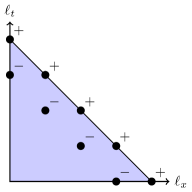
Figure 4: The sign contributions of the subspaces used for the combination technique for standard sparse grids with $\sigma=1$.

To introduce the combination technique we use the Galerkin projection onto the full tensor product discrete spaces. The Galerkin projection is well-defined due to the coercivity of the single-layer operator $V$.

Definition 4.10.

Let $\Pi_{\mathcal{X}}$ be a mapping

$$\Pi_{\mathcal{X}}\,:\,H^{-\frac{1}{2},-\frac{1}{4}}(\Sigma)\rightarrow\mathcal{X},$$

which satisfies Galerkin-orthogonality

$$\langle V(\varphi-\Pi_{\mathcal{X}}\varphi),v\rangle=0,~{}~{}~{}~{}\forall v\in\mathcal{X}.$$

We refer to this projection as the Galerkin projection. For ease of notation we will denote the Galerkin projection onto the space $\mathcal{X}_{\ell_{x}}^{x}\otimes\mathcal{X}_{\ell_{t}}^{t}$ by $\Pi_{\ell_{x},\ell_{t}}$.

Then for isotropic sparse grids we find indices such that

$$\ell_{x}+\ell_{t}=L-l,~{}l=0,1.$$ (27)

Running over these indices gives the combination technique sparse grid solution $\varphi_{L}$:

$$\varphi_{L}=\left(\sum_{l=0}^{L}\Pi_{l,L-l}\varphi-\sum_{l=0}^{L}\Pi_{l-1,L-l}\varphi\right)\in\mathcal{X}_{L}^{\sigma},~{}\sigma=1.$$ (28)

This combination of spaces is shown in Figure 4. Essentially one adds the spaces for $l=0$ (denoted by $+$ on the figure) and then subtracts the spaces for $l=1$ (denoted by $-$ on the figure).

If we want to use the combination technique for an anisotropic sparse grid index set, i.e. for a set of the form

$$\hat{I}_{L}^{\sigma}=\{(\ell_{x},\ell_{t})~{}:~{}\sigma\ell_{x}+\ell_{t}/\sigma\leq L\},$$

formula (27) is changed as follows (see [19])

$$\lceil\sigma^{2}l_{x}\rceil+\ell_{t}=\lceil\sigma L\rceil-l,~{}l=0,1.$$

4.2.1 Numerical Experiments

Next we test the convergence rates derived in Section 4, we compare the convergence rates of the square of the energy norm of the full tensor product discretisation and the isotropic sparse grid discretisation with a scaling of $\sigma=1$ in both. As before we chose the time horizon to be $T=4$ and solve the Dirichlet problem (1) on a unit circle with the right hand side $g(r,\varphi,t)=t^{2}\cos(\varphi)$.

The convergence rate for the full tensor product discretisation, namely $\frac{5}{8}$, is as expected. The expected convergence rate for the square of the energy norm for the isotropic sparse grid method is $\frac{7}{6}$. The tests in Figure 5 show a correspondence to the expected rates.

Lastly, we give some numerical results for the combination technique. The left plot in Figure 5 shows convergence of the energy norm against the total number of degrees of freedom. As expected, the convergence rates are identical to those obtained by implementing the sparse grid method using a multilevel decomposition. However, as the right plot in Figure 5 shows the combination technique provides a large improvement in the time taken for the calculation.

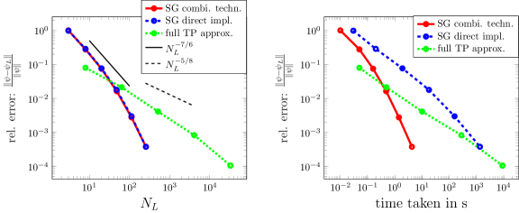
Figure 5: Convergence of the relative error in the energy norm squared versus number of degrees of freedom (left) and time taken in seconds (right) for the standard sparse grid space with the combination technique and without.

4.3 Adaptive Sparse Grids

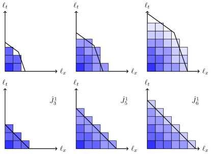
Figure 6: Growth of the adaptive index set shown by squares (top row). Darker squares denote the index set of earlier steps. The black line shows the a-priori index set $J_{L}^{\mathcal{T},\sigma}$. This is compared to the growth of the standard anisotropic sparse grid $\hat{J}_{L}^{\sigma}$ (bottom row).

Independently of the choice of approximation space $\hat{\mathcal{X}}_{L}$ we can make the following an Aubin-Nitsche argument. Let us assume that the solution $\psi$ is in $L^{2}(\Sigma)$.

$$\begin{split}\|\psi-\Pi_{\hat{\mathcal{X}}_{L}}\psi\|_{H^{-\frac{1}{2},-\frac{1}{4}}(\Sigma)}&=\sup_{\xi\in H^{\frac{1}{2},\frac{1}{4}}(\Sigma)}\frac{\langle\psi-\Pi_{\hat{\mathcal{X}}_{L}}\psi,\xi\rangle}{\|\xi\|_{H^{\frac{1}{2},\frac{1}{4}}(\Sigma)}}\\ &=\sup_{\xi\in H^{\frac{1}{2},\frac{1}{4}}(\Sigma)}\frac{\langle\psi-\Pi_{\hat{\mathcal{X}}_{L}}\psi,\xi-\Pi_{\hat{\mathcal{X}}_{L}}\xi\rangle}{\|\xi\|_{H^{\frac{1}{2},\frac{1}{4}}(\Sigma)}}\end{split}$$

Then we can estimate

$$\begin{split}&\|\psi-\Pi_{\hat{\mathcal{X}}_{L}}\psi\|_{H^{-\frac{1}{2},-\frac{1}{4}}(\Sigma)}\leq\|\psi-\Pi_{\hat{\mathcal{X}}_{L}}\psi\|_{L^{2}(\Sigma)}\sup_{\xi\in H^{\frac{1}{2},\frac{1}{4}}(\Sigma)}\frac{\|\xi-\Pi_{\hat{\mathcal{X}}_{L}}\xi\|_{L^{2}(\Sigma)}}{\|\xi\|_{H^{\frac{1}{2},\frac{1}{4}}(\Sigma)}}\\ &~{}~{}~{}~{}~{}\leq\|\psi\|_{H^{s_{x},s_{t}}_{\text{mix}}(\Sigma)}\underbrace{\frac{\|\psi-\Pi_{\hat{\mathcal{X}}_{L}}\psi\|_{L^{2}(\Sigma)}}{\|\psi\|_{H^{s_{x},s_{t}}_{\text{mix}}(\Sigma)}}}\underbrace{\sup_{\xi\in\|\psi\|_{H^{\frac{1}{2},\frac{1}{4}}(\Sigma)}}\frac{\|\xi-\Pi_{\hat{\mathcal{X}}_{L}}\xi\|_{L^{2}(\Sigma)}}{\|\xi\|_{H^{\frac{1}{2},\frac{1}{4}}(\Sigma)}}}\\ &~{}~{}~{}~{}~{}~{}~{}~{}~{}~{}~{}~{}~{}~{}~{}~{}~{}~{}~{}~{}~{}~{}~{}~{}~{}~{}~{}~{}~{}~{}\text{small for}~{}~{}~{}~{}~{}~{}~{}~{}~{}~{}~{}~{}~{}\text{small for full tensor}\\ &~{}~{}~{}~{}~{}~{}~{}~{}~{}~{}~{}~{}~{}~{}~{}~{}~{}~{}~{}~{}~{}~{}~{}~{}~{}~{}~{}~{}~{}~{}\text{standard}~{}~{}~{}~{}~{}~{}~{}~{}~{}~{}~{}~{}~{}~{}~{}\text{ product grids}\\ &~{}~{}~{}~{}~{}~{}~{}~{}~{}~{}~{}~{}~{}~{}~{}~{}~{}~{}~{}~{}~{}~{}~{}~{}~{}~{}~{}~{}~{}\text{sparse grids}\\ \end{split}$$

for any approximation space $\hat{\mathcal{X}}_{L}$. This argument leads to the idea of finding a compromise between the full tensor product discretisation and the sparse grid discretisation. However, it is unclear what form this index set should take. The optimised index sets given in [11] are one possibility. However, they still leave us several free parameters that need to be chosen.

In order to get a better idea of how a good index set might look we implemented a simple adaptive scheme from [16]. Since our aim was to gain a better understanding of the optimal shape of the index set, we have not used an error indicator to choose the next index to include. Instead we have simply calculated the actual contribution to the energy norm for each index.

For an index $(\ell_{x},\ell_{t})$ the local cost function $c(\ell_{x},\ell_{t})$ is given by the size of the corresponding subspace $W_{(\ell_{x},\ell_{t})}$, i.e.

$$c(\ell_{x},\ell_{t})=2^{\ell_{t}+l_{x}(d-1)}.$$

Our local benefit function $b(\ell_{x},\ell_{t})$ gives the contribution of the index to the energy norm, i.e.

$$b(\ell_{x},\ell_{t})=\|\psi_{(\ell_{x},\ell_{t})}\|_{H^{-\frac{1}{2},-\frac{1}{4}}(\Sigma)}.$$

In each step of the adaptive algorithm we choose the next admissible index that maximises the cost-benefit ratio $c(\ell_{x},\ell_{t})/b(\ell_{x},\ell_{t})$. We require that an admissible index has no “holes”, i.e. that all downset neighbours are already contained in the index set.

Figure 6 shows the growth of the adaptively chosen index set. We notice that these index sets behave similarly to the optimised index sets from [11] for negative choices of $\mathcal{T}$. For our purposes we require an anisotropy in the definition of the index sets. Care has to be taken when comparing to [11], where this anisotropy is not present in the definition.

Definition 4.11.

The optimised sparse grid index set is defined as follows

$$J_{L}^{\mathcal{T},\sigma}=\left\{(\ell_{x},\ell_{t})~{}:~{}\sigma\ell_{x}+l_{t}/\sigma-\mathcal{T}\max\{\sigma\ell_{x},\ell_{t}/\sigma\}\leq(1-\mathcal{T})L\right\}.$$

where $\mathcal{T}\in[-\infty,1)$and $\sigma$ are free variable .

The lines in Figure 6 show the boundary of the index set $J_{L}^{\mathcal{T},\sigma}$ for a scaling of $\frac{6}{5}$ and $\mathcal{T}=-1$ for comparison.

4.3.1 Numerical Experiments

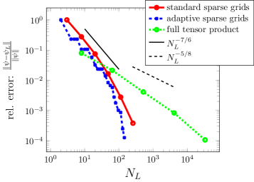
Figure 7: Convergence of the relative error in the energy norm squared versus number of degrees of freedom for the standard sparse grid space and for the adaptively chosen sparse grid space.

Next we numerically verify that the adaptively chosen index sets indeed yield an improvement over the standard index sets. In Figure 7 we see that this is the case. As before we chose the time horizon to be $T=4$ and solve the Dirichlet problem (1) on a unit circle with the right hand side $g(r,\varphi,t)=t^{2}\cos(\varphi)$. For this problem the exact solution is known, so the exact error can be calculated.

5 Conclusions

The boundary integral formulation efficiently approximates the Cauchy data of the given boundary value problem, i.e. the missing boundary values for the Neumann problem or the missing boundary fluxes for the Dirichlet problem. We have shown an error analysis for two types of discretisation spaces. Firstly, we have shown improved error bounds for a full tensor product discretisation. These improvements are largest for lower polynomial degrees, which are primarily of interest in an implementation.

Secondly, we have shown similar improvements for anisotropic sparse grid discretisation spaces. In terms of degrees of freedom the sparse grid discretisation gives a considerably higher convergence rates than the full tensor product discretisation. However, the sparse grid combination technique is essential to ensure that these gains lead to a corresponding speed-up in run time.

There is scope to explore the choice of sparse grid index set for this problem, as the adaptive algorithm shows that the anisotropic sparse grid index sets are not the optimal choice.

References

- [1] H. Wayland, Differential equations applied in science and engineering, D. Van Nostrand Co., Inc., Princeton, N. J.-Toronto-New York-London, 1957.
- [2] P. Wilmott, S. Howison, J. Dewynne, The Mathematics of Financial Derivatives, Cambridge University Press, 1995, cambridge Books Online.
- [3] A. Witkin, Scale-space filtering: A new approach to multi-scale description, in: Acoustics, Speech, and Signal Processing, IEEE International Conference on ICASSP 8́4., Vol. 9, 1984, pp. 150–153.
- [4] V. Thomee, Galerkin finite element methods for parabolic problems, Springer, 1984.
- [5] M. Griebel, D. Oeltz, A sparse grid space-time discretization scheme for parabolic problems, Computing 81 (1) (2007) 1–34.
- [6] M. Costabel, Boundary integral operators for the heat equation, Integral Equations Operator Theory 13 (4) (1990) 498–552.
- [7] A. Chernov, C. Schwab, Sparse space-time Galerkin BEM for the nonstationary heat equation, ZAMM Z. Angew. Math. Mech. 93 (2013) 403–413.
- [8] A. Chernov, C. Schwab, First order -th moment Finite Element analysis of nonlinear operator equations with stochastic data, Mathematics of Computation 82 (2013) 1859–1888.
- [9] M. Griebel, M. Schneider, C. Zenger, A combination technique for the solution of sparse grid problems, in: P. de Groen, R. Beauwens (Eds.), Iterative Methods in Linear Algebra, IMACS, Elsevier, North Holland, 1992, pp. 263–281.
- [10] J. Garcke, M. Griebel, On the computation of the eigenproblems of hydrogen and helium in strong magnetic and electric fields with the sparse grid combination technique, Journal of Computational Physics 165 (2) (2000) 694 – 716.
- [11] M. Griebel, S. Knapek, Optimized general sparse grid approximation spaces for operator equations, Math. Comp. 78 (268) (2009) 2223–2257.
- [12] P. Noon, The single layer heat potential and Galerkin boundary element methods for the heat equation, Phd thesis.
- [13] M. Griebel, H. Harbrecht, On the construction of sparse tensor product spaces, Mathematics of Computations 82 (282) (2013) 975–994.
- [14] A. Reinarz, Sparse space-time boundary element methods for the heat equation, Ph.D. thesis, University of Reading (2015).
- [15] C. Zenger, Sparse grids, Notes Numer. Fluid Mech. 31 (1991) 241–251.
- [16] H. Bungartz, M. Griebel, Sparse grids, Acta Numerica 13 (2004) 1–123.
- [17] M. Griebel, The combination technique for the sparse grid solution of PDEs on multiprocessor machines, Parallel Processing Letters 2 (1) (1992) 61–70.
- [18] M. Griebel, W. Huber, T. Störtkuhl, C. Zenger, On the parallel solution of 3D PDEs on a network of workstations and on vector computers, in: Lecture Notes in Computer Science 732, Parallel Computer Architectures: Theory, Hardware, Software, Applications, Springer Verlag, 1993, pp. 276–291.
- [19] M. Griebel, H. Harbrecht, On the convergence of the combination technique, in: Sparse grids and Applications, Vol. 97 of Lecture Notes in Computational Science and Engineering, Springer, 2014, pp. 55–74.