Optimization based evaluation of grating interferometric phase stepping series and analysis of mechanical setup instabilities

Abstract

The diffraction contrast modalities accessible by X-ray grating interferometers are not imaged directly but have to be inferred from sine like signal variations occurring in a series of images acquired at varying relative positions of the interferometer’s gratings. The absolute spatial translations involved in the acquisition of these phase stepping series usually lie in the range of only a few hundred nanometers, wherefore positioning errors as small as 10nm will already translate into signal uncertainties of one to ten percent in the final images if not accounted for.

Classically, the relative grating positions in the phase stepping series are considered input parameters to the analysis and are, for the Fast Fourier Transform that is typically employed, required to be equidistantly distributed over multiples of the gratings’ period.

In the following, a fast converging optimization scheme is presented simultaneously determining the phase stepping curves’ parameters as well as the actually performed motions of the stepped grating, including also erroneous rotational motions which are commonly neglected. While the correction of solely the translational errors along the stepping direction is found to be sufficient with regard to the reduction of image artifacts, the possibility to also detect minute rotations about all axes proves to be a valuable tool for system calibration and monitoring. The simplicity of the provided algorithm, in particular when only considering translational errors, makes it well suitable as a standard evaluation procedure also for large image series.

1 Introduction

X-ray grating interferometry [1, 2] facilitates access to new contrast modalities in laboratory X-ray imaging setups and has by now been implemented by many research groups after the seminal publication by Pfeiffer et al. in 2006 [3]. The additional information on X-ray refraction (“differential phase contrast”) and ultra small angle scattering (“darkfield contrast”) properties of a sample that can be obtained promises both increased sensitivity to subtle material variations as well as insights into the samples’ substructure below the spatial resolution of the acquired images.

In contrast to classic X-ray imaging, the absorption, differential phase and darkfield contrasts are not imaged directly but are encoded in sinusoidal intensity variations arising at each detector pixel when shifting the interferometer’s gratings relative to each other perpendicular to the beam path and the grating bars. A crucial step in the generation of respective absorption, phase and darkfield images therefore is the analysis of the commonly acquired phase stepping series, which shall be the subject of the present article. Respective examples are shown in Figures 1 and 2.

In principle, the images within such phase stepping series are sampled at about five to ten different relative grating positions equidistantly distributed over multiples of the gratings’ period such that the expected sinusoids for each detector pixel may be characterized by standard Fourier decomposition. The zeroth order term represents the mean transmitted intensity (as in classic X-ray imaging), while the first order terms encode phase shift and amplitude of the sinusoid. The ratio of amplitude and mean (generally referred to as “visibility”) is here related to scattering and provides the darkfield contrast. Higher order terms correspond to deviations from the sinusoid model mainly due to the actual grating profiles and are usually not considered.

Given typical grating periods in the range of two to ten micrometers, the actually performed spatial translations lie in the range of 200 to 2000 nanometers. Particular for the smaller gratings, positioning errors as small as 10 to 20 nm imply relative phase errors in the range of five to ten percent, causing uncertainties in the derived quantities in the same order of magnitude. The propagation of noise within the sampling positions onto the extracted signals has e.g. been studied by Revol et al. [4] and first results for the determination of the actual sampling positions from the available image series were shown by Seifert et al. [5] using methods by Vargas et al. [6] from the context of visible light interferometry. Otherwise the problem seems to have not been given much consideration so far.

The present article proposes a simple iterative optimization algorithm both for the fitting of irregularly sampled sinusoids and in particular also for the determination of the actual sampling positions. The use of only basic mathematical operations eases straightforward implementations on arbitrary platforms. Besides uncertainties in the lateral stepping motion, the remaining mechanical degrees of freedom (magnification/expansion and rotations) are also considered. The proposed techniques will be demonstrated on an exemplary data set.

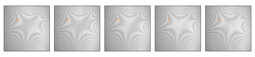
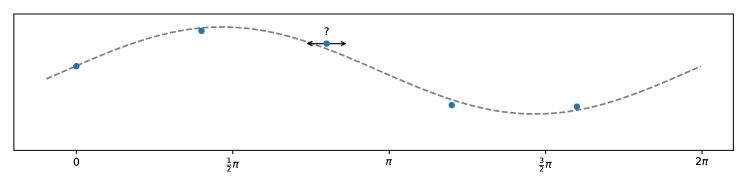
Figure 1: Example for a grating interferometric phase stepping series. The intensity variation throughout the series is visually most perceivable in the center. The spatial Moiré fringes are due to imperfectly matched gratings and will translate to reference offset phases of the sinusoid curves found at each detector pixel (cf. Fig. 2). The bottom row shows a corresponding phase stepping curve for the pixel marked orange in the above image series. The sampling positions are subject to an unknown error.

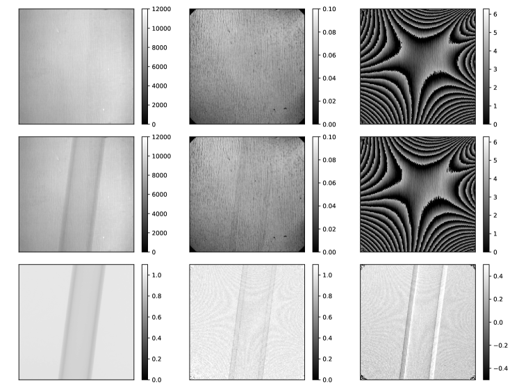
Figure 2: From left to right: transmission (sinusoid mean), visibility (ratio of sinusoid amplitude and mean) and phase images derived from phase stepping series as shown in Fig. 1. The first rows show acquisitions with and without sample, while the last row shows the sample images (center row) normalized with respect to the empty beam images (first row). Positioning errors in the phase stepping procedure cause the Moiré pattern of the reference phase image to translate into the final results.

2 Methods

The task of sinusoid fitting with imprecisely known sampling locations will be partitioned into two separate optimization problems considering either only the sinusoid parameters or only the sampling positions while temporarily fixing the respective other set of parameters. Alternating both optimization tasks will minimize the joint objective function in few iterations.

2.1 Sinusoid Fitting

A simple iterative forward-backprojection algorithm converging to the least squares solution can be derived when representing the sinusoid model as a linear combination of basis functions:

$$o+a\sin(\phi-\phi_{0}) =o+a\left(\cos\phi_{0}\sin\text{$\phi$}-\sin\phi_{0}\cos\phi\right)$$ (1)

$$=o+a_{s}\sin\phi+a_{c}\cos\phi$$

$$=(o,a_{s},a_{c})\cdot(1,\sin\phi,\cos\phi)^{T}$$

with the following identities:

$$a =\sqrt{a_{s}^{2}+a_{c}^{2}}$$ (2)

$$\sin\phi_{0} =-a_{c}/a$$

$$\cos\phi_{0} =a_{s}/a$$

$$\phi_{0} =\arctan\!2(-a_{c},a_{s})\,.$$

The components $o$, $a_{c}$, $a_{s}$ may be determined by means of the following iterative scheme (introducing the sample index $i$ and the superscript iteration index $k$):

$$o^{(0)},a_{c}^{(0)},a_{s}^{(0)} =0,0,0$$ (3)

$$\tilde{y}_{i}^{(k)} =o^{(k)}+a_{c}^{(k)}\cos\phi_{i}+a_{s}^{(k)}\sin\phi_{i}$$

$$o^{(k+1)} =o^{(k)}+\frac{1}{N}\sum_{i}(y_{i}-\tilde{y}_{i}^{(k)})$$

$$a_{s}^{(k+1)} =a_{s}^{(k)}+\frac{2}{N}\sum_{i}(y_{i}-\tilde{y}_{i}^{(k)})\sin\phi_{i}$$

$$a_{c}^{(k+1)} =a_{c}^{(k)}+\frac{2}{N}\sum_{i}(y_{i}-\tilde{y}_{i}^{(k)})\cos\phi_{i}$$

where the factors of $1/N$ and $2/N$ account for the normalization of the respective basis functions (with $N$ being the amount of samples $(\phi_{i},y_{i})$ enumerated by $i$). The scheme reduces to classic Fourier analysis for the case of the abscissas $\phi_{i}$ being equidistantly distributed over multiples of $2\pi$ and converges within the first iteration in that case. As the update terms to $o$, $a_{c}$ and $a_{s}$ are proportional to the respective derivatives of the $\ell_{2}$ error $\sum_{i}(o^{(k)}+\,a_{c}^{(k)}\!\cos\phi_{i}\,+\,a_{s}^{(k)}\!\sin\phi_{i}\,-y_{i})^{2}$, the fixpoint of the iteration will be the least squares fit also in all other cases.

For a stopping criterion, the relative error reduction

$$\Delta_{\ell_{2}}=\frac{\sqrt{\sum_{i}^{N}\left(y_{i}-\tilde{y}_{i}^{(k-1)}\right)^{2}}-\sqrt{\sum_{i}^{N}\left(y_{i}-\tilde{y}_{i}^{(k)}\right)^{2}}}{\sqrt{\sum_{i}^{N}\left(y_{i}-\tilde{y}_{i}^{(k)}\right)^{2}}}$$ (4)

may be tracked. It is typically found to fall below 0.1% within 10 to 20 iterations given only slightly noisy data (noise sigma three orders of magnitude smaller than sinusoid amplitude) and within less than 10 iterations for most practical cases. For the special case of equidistributed $\phi_{i}$ on multiples of $2\pi$, it will immediately drop to 0 after the first iteration. In practice, a fixed amount of iterations in the range of five to fifteen will therefore be adequate as stopping criterion as well.

2.2 Phase Step Optimization

An underlying assumption of the previously described least squares fitting procedure is the certainty of the abscissas, i.e. the set of phases $\phi_{i}$ at which the ordinates $y_{i}$ have been sampled. As the sampling positions are themselves subject to experimental uncertainties (arising from the mechanical precision of the involved actuators), a further optimization step will be introduced that minimizes the least squares error of the sinusoid fit over the sampling positions $\phi_{i}$. While this procedure obviously results in overfitting when considering only a single phase stepping curve (PSC), it becomes a well-defined error minimization problem when regarding large sets of PSCs sharing the same $\phi_{i}$. In other words, an approach to the minimization of the objective function

$$o_{j},a_{j},\phi_{0,j},\Delta\phi_{i}=\underset{o_{j},a_{j},\phi_{0,j},\Delta\phi_{i}}{\text{argmin}}\sum_{i,j}\left(o_{j}+a_{j}\sin(\phi_{i}+\Delta\phi_{i}-\phi_{0_{j}})-y_{ij}\right)^{2}$$ (5)

shall be considered, where $j$ indexes detector pixels.

In order to derive an optimization procedure for the sampling positions, first the fictive case of a perfectly sinusoid PSC with negligible statistical error on the ordinate (the sampled values) shall be considered. Ignoring for now the fact that least squares fits commonly assume only the ordinates to be affected by noise, a least squares fit shall be used to preliminarily determine the parameters of the sinusoid described by the observed data. Assuming then that inconsistencies of the observed data with the model are due to errors on the sampling locations, deviations from their intended positions are given by the data points’ lateral distances from the sinusoid curve (cf. Fig. 3). Finally, the actual systematic deviations of the sampling locations can be found by averaging over the respective results for a large set of PSCs sampled simultaneously. This information can be fed back into the original sinusoid fit, which then again allows the refinement of the current estimate of the true sampling positions, finally resulting in an iterative procedure alternatingly optimizing the sinusoid parameters and the actual sampling locations (cf. Algorithm 1).

2.2.1 Determination of individual phase deviations

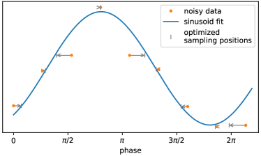
Figure 3: Optimization of the actual (in contrast to the intended) sampling positions by Eq. 13 with respect to a previous sinusoid fit based on the temporary assumption that deviations from the sinusoid model are mainly due to errors on the sampling positions rather than the sampled ordinate values. Averaging of respective phase deviations found for large sets of measurements will finally allow the differentiation of systematic deviations from statistical noise (see also Fig. 6).

Starting with an initial sinusoid fit

$$o,a,\phi_{0}=\underset{o,a,\phi_{0}}{\text{argmin}}\sum_{i}\left(o+a\sin(\phi_{i}-\phi_{0})-y_{i}\right)^{2}\,,$$ (6)

the error shall be minimized over deviations $\Delta\phi_{i}$ to $\phi_{i}$ while keeping the sinusoid model parameters fixed:

$$\Delta\phi_{i}=\underset{\Delta\phi_{i}}{\text{argmin}}\sum_{i}\left(o+a\sin(\phi_{i}+\Delta\phi_{i}-\phi_{0})-y_{i}\right)^{2}\,.$$ (7)

Equation 7 is solved when the derivative of the objective function with respect to $\Delta\phi_{i}$ vanishes:

$$0 =\frac{\text{d}}{\text{d}\Delta\phi_{i}}\sum_{i}\left(o+a\sin(\phi_{i}+\Delta\phi_{i}-\phi_{0})-y_{i}\right)^{2}$$ (8)

$$0 =2\left(o-y_{i}+a\sin(\phi_{i}+\Delta\phi_{i}-\phi_{0})\right)a\cos(\phi_{i}+\Delta\phi_{i}-\phi_{0})$$

$$\text{for }a\cos(\phi_{i}+\Delta\phi_{i}-\phi_{0})\neq 0:$$

$$0 =\left(o-y_{i}+a\sin(\phi_{i}+\Delta\phi_{i}-\phi_{0})\right)$$

$$\text{for }\Delta\phi_{i}\ll\pi:$$

$$0 \approx\left(o-y_{i}+a\sin(\phi_{i}-\phi_{0})+\Delta\phi_{i}a\cos(\phi_{i}-\phi_{0})\right)$$

where the last step is a first order Taylor expansion with respect to $\Delta\phi_{i}$. This directly leads to the following expression for $\Delta\phi_{i}$:

$$\Delta\phi_{i}\approx\frac{1}{\cos(\phi_{i}-\phi_{0})}\left(\frac{y_{i}-o}{a}-\sin(\phi_{i}-\phi_{0})\right)\quad\quad\text{for }\Delta\phi_{i}\ll\pi\text{ and }a\cos(\phi_{i}-\phi_{0})\neq 0\,\,,$$ (9)

where the earlier condition $a\cos(\phi_{i}+\Delta\phi_{i}-\phi_{0})\neq 0$ is approximated to be satisfied when $a\cos(\phi_{i}-\phi_{0})\neq 0$. The restriction to cases with $a\cos(\phi_{i}-\phi_{0})\neq 0$ can be intuitively understood when recalling that $\cos(\phi_{i}-\phi_{0})=0$ implies a maximum or minimum of the sinusoid and $a=0$ means that it is constant ($\phi_{i}$ independent), in both of which cases there is no sensible choice for $\Delta\phi_{i}\neq 0$. The constraint on the result, $\Delta\phi_{i}\ll\pi$, can simply be taken into account by means of a limiting function such as

$$\text{softlimit}(\Delta\phi_{i},m\geq 0) =\begin{cases}0&m=0\\ m\tanh\left(\frac{\Delta\phi_{i}}{m}\right)&\text{else}\end{cases}\,\,,$$ (10)

which provides a linear mapping with slope $1$ for $\Delta\phi_{i}\ll m$ and is bounded at $\pm m$. The choice of $m$ in this case depends on the validity range of the linear approximation of $\sin(\phi_{i}+\Delta\phi_{i}-\phi_{0})$ with respect to $\Delta\phi_{i}$ about $\phi_{i}-\phi_{0}$, which obviously depends on the magnitude of the curvature of the sinusoid at this point as illustrated in Figure 4. The latter may be accounted for by

$$m=m_{\phi_{i}-\phi_{0}}=m_{0}\cos^{2}(\phi_{i}-\phi_{0})$$ (11)

which reaches its maximum $m_{\phi_{i}-\phi_{0}}=m_{0}$ at $\phi_{i}-\phi_{0}=0$ (where $\sin(\phi_{i}-\phi_{0})$ is actually linear) and smoothly drops to $0$ for $\cos(\phi_{i}-\phi_{0})=0$, in which case both the sine and its curvature are maximal and $\Delta\phi_{i}$ shall remain $0$. The actual choice of $m_{0}$ can now be based on the validity range of the linear approximation about $\phi_{i}-\phi_{0}=0$. The upper bound to $m_{\phi_{i}-\phi_{0}}$ and thus to $m_{0}$ is defined by the range over which $\sin(x-x_{0}),\,x\in[-m_{0}\cos^{2}(x_{0}),+m_{0}\cos^{2}(x_{0})]$ is actually invertible (cf. Fig. 4), i.e.:

$$m_{0}\cos^{2}(\phi) \leq\frac{\pi}{2}-|\phi|$$ (12)

$$m_{0} \lesssim 1.38\,.$$

For $m_{0}=1.38$, the linear approximation used in Eq. 8 deviates by up to $40\%$. The deviation is reduced to $20\%$ or $5\%$ for $m_{0}=1$ and $m_{0}=\frac{1}{2}$ respectively.

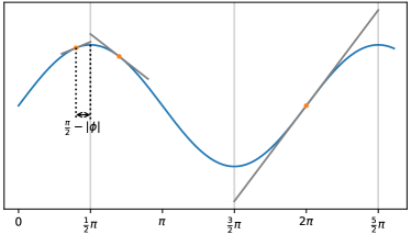
Figure 4: Illustration of the maximal sensible ranges for linear approximations of a sinusoid. Vertical lines at the turning points indicate the boundaries of monotone sections that should never be crossed by linear approximations of the curve. The maximum meaningful range is thus largest for points furthest from these boundaries and reduces to zero exactly at the turning points. Equation 11 approximates this phase dependence of the validity range with a $\cos^{2}$ function, and Eq. 12 defines the maximum amplitude admissible in order to indeed never exceed turning points.

Combining the above results and introducing for completeness also the detector pixel index $j$, the following expression for $\Delta\phi_{ji}$ reducing (and, for sufficiently small $\Delta\phi_{ji}$, minimizing) the $\ell_{2}$ error $\left(o_{j}+a_{j}\sin(\phi_{i}+\Delta\phi_{ji}-\phi_{0,j})-y_{ji}\right)^{2}$ can be given, choosing $m_{0}=\frac{1}{2}$:

$$\Delta\phi_{ji}\approx\begin{cases}0&a\cos(\phi_{i}-\phi_{0,j})=0\\ \text{softlimit}\left(\frac{\left(\frac{y_{ji}-o_{j}}{a_{j}}-\sin(\phi_{i}-\phi_{0,j})\right)}{\cos(\phi_{i}-\phi_{0,j})},\frac{1}{2}\cos^{2}(\phi_{i}-\phi_{0,j})\right)&\text{else}\end{cases}\,\,,$$ (13)

Figure 3 shows an example of this approximate least squares solution to $\Delta\phi_{ji}$.

2.2.2 Noise weighted average of phase deviations

Now that an expression has been derived for the deviations $\Delta\phi_{ji}$ optimizing the abscissa values for a single PSC given a previous sinusoid fit, the respective results for many PSCs (indexed by $j$) sharing the same sampling locations may be averaged:

$$\Delta\phi_{i}=\frac{\sum_{j}w_{ji}\Delta\phi_{ji}}{\sum_{j}w_{ji}}\,,$$ (14)

using weights $w_{ji}$ factoring in the relative certainty and relevance of the different $\Delta\phi_{ji}$. An appropriate choice is

$$w_{ji}=a_{j}^{2}\cos^{2}(\phi_{i}-\phi_{0,j})\,,$$ (15)

where $\cos^{2}(\phi_{i}-\phi_{0,j})$ weights the slope dependent error propagation from noisy measurements $y_{ji}$ to $\Delta\phi_{ji}$ based on the derivative of the sinusoid model at $\phi_{i}$ and $a_{j}^{2}$ weights the contribution of a particular PSC $j$ to the accumulated $\ell_{2}$ error. These considerations lead to

$$\Delta\phi_{i} =\frac{\sum_{j}a_{j}^{2}\cos^{2}(\phi_{i}-\phi_{0,j})\Delta\phi_{ji}}{\sum_{j}a_{j}^{2}\cos^{2}(\phi_{i}-\phi_{0,j})}$$ (16)

$$=\frac{\sum_{j}a_{j}^{2}\cos^{2}(\phi_{i}-\phi_{0,j})\text{softlimit}\left(\frac{\left(\frac{y_{ji}-o_{j}}{a_{j}}-\sin(\phi_{i}-\phi_{0,j})\right)}{\cos(\phi_{i}-\phi_{0,j})},\frac{1}{2}\cos^{2}(\phi_{i}-\phi_{0,j})\right)}{\sum_{j}a_{j}^{2}\cos^{2}(\phi_{i}-\phi_{0,j})}$$

$$=\frac{\sum_{j}\text{softlimit}\left(\cos(\phi_{i}-\phi_{0,j})\left(a_{j}(y_{ji}-o_{j})-a_{j}^{2}\sin(\phi_{i}-\phi_{0,j})\right),\frac{1}{2}a_{j}^{2}\cos^{4}(\phi_{i}-\phi_{0,j})\right)}{\sum_{j}a_{j}^{2}\cos^{2}(\phi_{i}-\phi_{0,j})}\,\,,$$

where the last step uses the relation $\alpha\,\text{softlimit}(x,m)=\text{softlimit}(\alpha x,\alpha m)$ for $\alpha\geq 0$.

Finally, the above derivations can be combined to an iterative optimization algorithm reducing the accumulated least square error of multiple sinusoid fits (indexed by $j$) to data points $y_{ji}$ over shared abscissa values $\phi_{i}$ as defined by Equation 5. A pseudo code representation is given in Alg. 1, further introducing the relaxation parameter $\text{$\lambda$}_{k}\in(0;1]$ that may be chosen $<1$ in order to damp the adaptions to $\phi_{i}^{(k)}$ if desired. The intermediate sinusoid fits may be accomplished using the iterative algorithm described in the previous section.

1:${\phi_{i}},{y_{ji}}$: input data

2:$m_{0}\leftarrow\frac{1}{2}$ $\triangleright$ upper limit to $\Delta\phi_{ji},m_{0}\in(0;1.38]$

3:$\phi_{i}^{(0)}\leftarrow\phi_{i}$

4:$o_{j}^{(0)},a_{j}^{(0)},\phi_{0,j}^{(0)}\leftarrow\underset{o,a,\phi_{0}}{\text{argmin}}\sum_{i}\left(o+a\sin(\phi_{i}^{(0)}-\phi_{0})-y_{ji}\right)^{2}$ $\triangleright$ initalization

5:for $k=0\,..\,k_{\max}$ do

6:     $\Delta\phi_{i}^{(k)}\leftarrow\frac{\sum_{j}\text{softlimit}\left(\cos(\phi_{i}^{(k)}-\phi_{0,j}^{(k)})\left(a_{j}^{(k)}(y_{ji}-o_{j}^{(k)})-a_{j}^{2}\sin(\phi_{i}^{(k)}-\phi_{0,j}^{(k)})\right),(a_{j}^{(k)})^{2}m_{0}\cos^{4}(\phi_{i}^{(k)}-\phi_{0,j}^{(k)})\right)}{\sum_{j}(a_{j}^{(k)})^{2}\cos^{2}(\phi_{i}^{(k)}-\phi_{0,j}^{(k)})}$

7:     $\phi_{i}^{(k+1)}\leftarrow\phi_{i}^{(k)}+\lambda_{k}\Delta\phi_{i}^{(k)}$

8:     $o_{j}^{(k+1)},a_{j}^{(k+1)},\phi_{0,j}^{(k+1)}\leftarrow\underset{o_{j},a_{j},\phi_{0,j}}{\text{argmin}}\sum_{i}\left(o_{j}+a_{j}\sin(\phi_{i}^{(k+1)}-\phi_{0,j})-y_{ji}\right)^{2}$

9:end for.

Algorithm 1 Least squares optimization of shared abscissa values $\phi_{i}$ for simultaneous sinusoid fits to ordinate samples $y_{ji}$ belonging to independent curves $j$ sampled at identical positions $\phi_{i}$. This represents a special case of Algorithm 2 with spatially invariant sampling phases. The relaxation parameter $\lambda_{k}\in(0;1]$ may be chosen $<1$ if damping of the updates to $\phi_{i}^{(k)}$ is desired. For the intermediate argmin operations see Equations 1–4.

2.2.3 Inhomogeneous sampling phase deviations

Up to now, it has been assumed that deviations from the intended phase stepping positions are due to purely translational uncertainties in the relative motion of the involved gratings, resulting in offsets $\Delta\phi_{i}$ of the actual from the intended sampling phases that are homogeneous throughout the whole detection area. When also considering relative grating period changes (e.g. due to either thermal expansion or motion induced changes in magnification) and rotary motions of the interferometer’s gratings relative to each other (e.g. due to backlashes within the mechanical actuators), the effective sampling phases at each phase step may exhibit gradients over the detection area. Given the small grating periods (micrometer scale) compared to the total extents of the gratings (centimeter scale), both tilts in the sub-microrad range and relative period changes in the range of $10^{-7}$ will already manifest themselves in observable gradients.

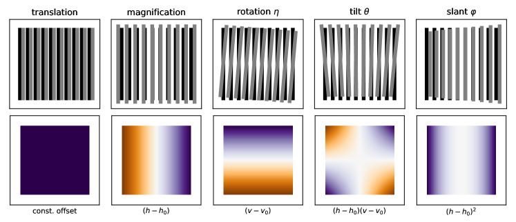
Figure 5: Grating misalignments (top row) and corresponding spatial phase variations (bottom row). From left to right: translation, magnification, rotation, tilt, slant. The latter two effects (as well as translation induced magnification) are only observable in cone beam setups. The employed colorbar ranges from orange for negative values over white (zero) to blue for positive values.

The corresponding optimization problem regarding also gradients is, analog to Equation 5, given by:

$$o_{j},a_{j},\phi_{0,j},\Delta\phi_{i}(j)=\underset{o_{j},a_{j},\phi_{0,j},\Delta\phi_{i}(j)}{\text{argmin}}\sum_{i,j}\left(o_{j}+a_{j}\sin(\phi_{i}+\Delta\phi_{i}(j)-\phi_{0_{j}})-y_{ij}\right)^{2}$$ (17)

where the spatial dependence of the phase deviations $\Delta\phi_{i}$ has been accounted for by a functional dependence on the detector pixel index $j$. Given the expected gradients (as illustrated in Figure 5), $\Delta\phi_{i}(j)$ has the following form:

$$\Delta\phi_{i}(j)=\Delta\phi_{i}+\nabla_{\!h}\phi_{i}\,(h-h_{0})+\nabla_{\!v}\phi_{i}\,(v-v_{0})+\nabla_{\!hv}\phi_{i}(h-h_{0})(v-v_{0})+\nabla_{\!h}^{2}\phi_{i}(h-h_{0})^{2}\,,$$ (18)

with $\nabla_{\!h}\phi_{i}$, $\nabla_{\!v}\phi_{i}$, $\nabla_{\!hv}\phi_{i}$ and $\nabla_{\!h}^{2}\phi_{i}$ quantifying the respective gradients in horizontal and vertical direction as well as the mixed term and the curvature in horizontal direction, and $h$ and $v$ being spatial detector pixel indices related to the linear pixel index $j$ through the amount $N_{h}$ of pixels within one detector row:

$$j =vN_{h}+h$$ (19)

$$h =j\bmod N_{h}$$

$$v =(j-h)/N_{h}\,.$$

The constant offsets $h_{0}$ and $v_{0}$ characterize the detector center.

The optimization of the extended objective function in Equation 17 can be performed analog to that of Eq. 5 with the only difference lying in the evaluation of the spatial phase difference maps $\Delta\phi_{ji}$ defined by Eq. 13 (an example of which is shown in Figure 6). The weighted average derived in the previous section in order to determine the homogeneous offset $\Delta\phi_{i}$ can be extended to a generalized linear least squares fit of the model $\Delta\phi_{i}(j)=\Delta\phi_{i}(h(j),v(j))$ defined by Eq. 18 to the local estimates $\Delta\phi_{ij}$ (Eq. 13, Fig. 6), also taking the weights defined by Eq. 15 into account. Said procedure is stated more formally in Algorithm 2.

Basic geometric considerations neglecting higher order interrelations of the considered effects (e.g. rotation and effective period change) result in the following relations between the observable parameters $\nabla_{\!h}\phi_{i}$, $\nabla_{\!v}\phi_{i}$, $\nabla_{\!hv}\phi_{i}$, $\nabla_{\!h}^{2}\phi_{i}$ and relative translatory and rotatory motions of the interferometer’s gratings. In order to relate various magnification changes to spatial motions based on the intercept theorem, an assumption has to be made as to which of the gratings actually moved. Here, the grating that is mounted on the linear phase stepping actuator is assumed to be the cause of all relative motions of both gratings also including tilts and rotations. The “source–grating distance” in the following equations will thus refer to the stepped grating.

$\Delta\phi_{i}$ quantifies the translational error analog to Section 2.2.2. In contrast to the previous section, the present model distinguishes between homogeneous phase deviations induced by translation and the mean component induced by the $\nabla_{\!h}^{2}\phi_{i}(h-h_{0})^{2}$ term in the case of non-vanishing curvature of the spatial phase deviation.

The vertical gradient parameter $\nabla_{\!v}\phi_{i}$ is related to a relative rotation $\eta$ of both gratings about the optical axis:

$$\tan\eta =\frac{\nabla_{\!v}\phi_{i}}{2\pi}\frac{\text{effective grating period}}{\text{detector pixel pitch}}\,,$$ (20)

where the “effective grating period” refers to the projected period length at the location of the detector, which should be identical for both interferometer gratings (not considering the optional additional coherence grating close to the X-ray source).

The horizontal gradient parameter $\nabla_{\!h}\phi_{i}$ is related to a relative mismatch in effective grating periods of the gratings either due to relative distance changes along the optical axis or due to actual expansions (e.g. thermally induced):

$$\text{relative period mismatch}=\frac{\text{effective period difference}}{\text{effective grating period}}=\frac{\nabla_{\!h}\phi_{i}}{2\pi}\frac{\text{effective grating period}}{\text{detector pixel pitch}}\,.$$ (21)

When assuming relative grating period mismatches to be caused by changes in magnification due to translations of one of the gratings along the optical axis, the following relation applies to first order:

translation distance $$=(\text{relative period mismatch})\frac{(\text{source--grating distance})^{2}}{\text{source--detector distance}}$$ (22)

$$=\frac{\nabla_{\!h}\phi_{i}}{2\pi}\frac{\text{effective grating period}}{\text{detector pixel pitch}}\frac{(\text{source--grating distance})^{2}}{\text{source--detector distance}}\,.$$

The change $\nabla_{\!hv}\phi_{i}$ of the horizontal gradient throughout the vertical direction corresponds to a relative change in magnification from top to bottom, e.g. due to a tilt $\theta$ of one of the gratings about the horizontal axis. Using the above relation between magnification changes and spatial displacements, the tilt $\theta$ about the horizontal axis is related to $\nabla_{\!hv}\phi_{i}$ approximately by

$$\tan\theta =\frac{\nabla_{\!hv}\phi_{i}}{2\pi}\frac{\text{effective grating period}}{\text{detector pixel pitch}}\left((\text{detector pixel pitch})\frac{\text{source--grating distance}}{\text{source--detector distance}}\right)^{-1}\times$$ (23)

$$\quad\quad\quad\quad\quad\quad\quad\quad\quad\quad\quad\quad\quad\quad\quad\quad\quad\quad\quad\quad\quad\quad\quad\quad\quad\times\frac{(\text{source--grating distance})^{2}}{\text{source--detector distance}}$$

$$=\frac{\nabla_{\!hv}\phi_{i}}{2\pi}\frac{(\text{effective grating period})(\text{source--grating distance})}{(\text{detector pixel pitch})^{2}}\,.$$

A non-vanishing curvature $\nabla_{\!h}^{2}\phi_{i}$ arises in case of a rotary motion about the vertical axis (slant) and is analogously related to the slant angle $\varphi$ to first order by

$$\tan\varphi=\frac{\nabla_{\!h}^{2}\phi_{i}}{2\pi}\frac{(\text{effective grating period})(\text{source--grating distance})}{(\text{detector pixel pitch})^{2}}\,.$$ (24)

1:${\phi_{i}},{y_{ji}}$: input data

2:$m_{0}\leftarrow\frac{1}{2}$ $\triangleright$ upper limit to $\Delta\phi_{ji},m_{0}\in(0;1.38]$

3:$\phi_{ji}^{(0)}\leftarrow\phi_{i}\forall j$ $\triangleright$ initialization of sampling phases with intended values

4:$o_{j}^{(0)},a_{j}^{(0)},\phi_{0,j}^{(0)}\leftarrow\underset{o,a,\phi_{0}}{\text{argmin}}\sum_{i}\left(o+a\sin(\phi_{i}^{(0)}-\phi_{0})-y_{ji}\right)^{2}$ $\triangleright$ initial sinusoid fits

5:for $k=0\,..\,k_{\max}$ do

6:     $\Delta\phi_{ji}^{(k)}\leftarrow\begin{cases}0&a_{j}^{(k)}\cos(\phi_{ji}^{(k)}-\phi_{0,j}^{(k)})=0\\ \text{softlimit}\left(\frac{(y_{ji}-o_{j}^{(k)})/a_{j}^{(k)}-\sin(\phi_{ji}^{(k)}-\phi_{0,j}^{(k)})}{\cos(\phi_{ji}^{(k)}-\phi_{0,j}^{(k)})},m_{0}\cos^{2}(\phi_{ji}^{(k)}-\phi_{0,j}^{(k)})\right)&\text{else}\end{cases}$

7:     $w_{ji}^{(k)}\leftarrow a_{j}^{(k)\,2}\cos^{2}(\phi_{ji}^{(k)}-\phi_{0,j}^{(k)})$

8:     $\Delta\phi_{i}^{(k)},\nabla_{\!h}\phi_{i}^{(k)},\nabla_{\!v}\phi_{i}^{(k)},\nabla_{\!hv}\phi_{i}^{(k)},\nabla^{2}_{\!h}\phi_{i}^{(k)}\leftarrow$ $\underset{\Delta\phi_{i},\nabla_{\!h}\phi_{i},\nabla_{\!v}\phi_{i},\nabla_{\!hv}\phi_{i},\nabla^{2}_{\!h}\phi_{i}}{\mathrm{argmin}}\sum_{j}w_{ji}\left(\Delta\phi_{i}(j)-\Delta\phi_{ji}^{(k)}\right)^{2}$ $\triangleright$ for $\Delta\phi_{i}(j)$, cf. Eq. 18

9:     $\phi_{ji}^{(k+1)}\leftarrow\phi_{ji}^{(k)}+\Delta\phi_{i}^{(k)}+\nabla_{\!h}\phi_{i}^{(k)}\,(h-h_{0})+\nabla_{\!v}\phi_{i}^{(k)}\,(v-v_{0})+\nabla_{\!hv}\phi_{i}^{(k)}\,(h-h_{0})(v-v_{0})+\nabla^{2}_{\!h}\phi_{i}^{(k)}\,(h-v_{0})^{2}$

10:     $o_{j}^{(k+1)},a_{j}^{(k+1)},\phi_{0,j}^{(k+1)}\leftarrow\underset{o_{j},a_{j},\phi_{0,j}}{\mathrm{argmin}}\sum_{i}\left(o_{j}+a_{j}\sin(\phi_{ji}^{(k+1)}-\phi_{0,j})-y_{ji}\right)^{2}$

11:end for.

Algorithm 2 Simultaneous least squares optimization of abscissa values $\phi_{ji}$ and sinusoid fits to ordinate samples $y_{ji}$ belonging to independent curves $j$ sampled at positions $\phi_{ji}=\phi_{i}(j)$ with $\phi_{i}(j)$ being a slowly varying polynomial with respect to the spatial coordinates $h(j)$ and $v(j)$ accounting for the expected effects due to translations, magnification and rotations of an interferometer’s gratings. The procedure reduces to Algorithm 1 when considering only the zeroth order term of $\phi_{i}(j)$.

3 Experiment and Results

Figure 6: Example of phase differences (left) obtained from Equation 13 (cf. also Fig. 3) for the first frame of the phase stepping series shown in Fig. 1 with corresponding importance weights (right) as defined by Eq. 15. White regions (0 on the colorbar) in the left hand side $\Delta\phi$ map correspond to samples close to or exactly on turning points of the fitted sinusoids, where phase differences cannot be effectively determined. These areas get little weighting in the determination of the average phase deviation as can be seen by the corresponding dark fringes in side weighting map on the right.

$\sqrt{\overline{\Delta\phi_{i}^{2}}}$	$\sqrt{\overline{\left(\nabla_{\!h}\phi_{i}(h-h_{0})\right)^{2}}}$	$\sqrt{\overline{\left(\nabla_{\!v}\phi_{i}(v-v_{0})\right)^{2}}}$	$\sqrt{\overline{\left(\nabla_{\!hv}\phi_{i}(h-h_{0})(v-v_{0})\right)^{2}}}$	$\sqrt{\overline{\left(\nabla_{\!h}^{2}\phi_{i}(h-h_{0})^{2}\right)^{2}}}$
$1.2\times 10^{-1}$	$2.4\times 10^{-3}$	$3.6\times 10^{-3}$	$3.6\times 10^{-4}$	$7.5\times 10^{-4}$

Table 1: Root mean square contributions of the gradient and curvature components of $\Delta\phi_{i}(j)$ to the sampling phase deviations found for the present phase stepping series in units of radians. The homogeneous error $\Delta\phi$ is by far the dominating effect. The contributions of $\nabla_{\!hv}\phi$ and $\nabla_{\!h}^{2}\phi$ range in the order of magnitude of the expected noise level of $10^{-4}\,\text{rad}$ (cf. Eqs. 25, 26).

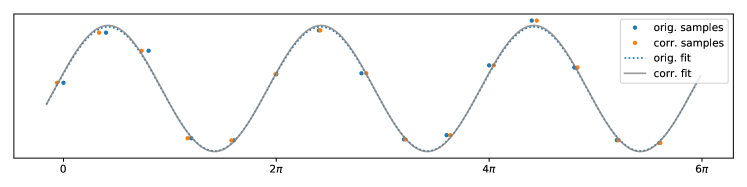
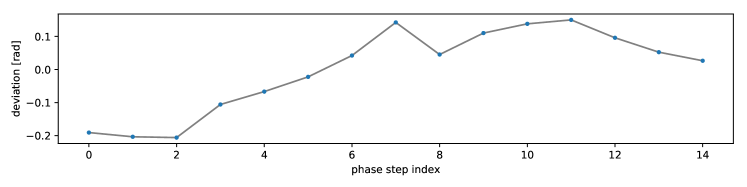
Figure 7: Above: An exemplary phase stepping curve consisting of 15 steps over three grating periods. Sampled values are shown both at the originally intended as well as at the inferred sampling positions (blue and orange markers respectively) along with the corresponding initial and corrected sinusoid fits. Although the difference in the resulting fit appears small, it is clearly noticeable in the final images as shown in Fig. 8.    Below: Deviations of the phase stepping series’ sampling positions from the intended ones in units of radians. The range of deviations corresponds to roughly $\pm 10\%$ of the intended stepping increments of $\frac{2}{5}\pi$.

Phase stepping series of 15 images sampled at varying relative grating shifts uniformly distributed over three grating periods have been acquired both with and without sample in the beam path. Figure 1 shows the first five frames of the empty beam series. The resulting phase stepping curves at each pixel (indexed by $j$) of the detector have been evaluated using a least squares fit to a sinusoid model parameterized by mean $o_{j}$, amplitude $a_{j}$ and phase offset $\phi_{0,j}$ under the initial assumption of perfectly stepped gratings. These preliminary results are shown in Figure 2 and correspond to those obtained by classic Fourier analysis of the phase stepping curves. Deviations of the sampling positions from the intended ones are then determined based on systematic deviations of the sampled data from the fitted sinusoids by means of Eq. 16 for all 15 frames of the phase stepping series. Figure 6 shows an exemplary result for the first frame of the series. Iterating the sinusoid fits and the corrections to the sampling positions in order to reduce the overall least squares error (cf. Equation 5) by means of Algorithm 1, the sampling positions’ deviations are found as shown in Figure 7. Figure 8 shows the reduction of Moiré modulated systematic errors in the final results, i.e. the transmission, visibility and differential phase images. The root mean square error is reduced by almost a factor of two in the present example and is already close to convergence after the first iteration as can be seen in Fig. 9.

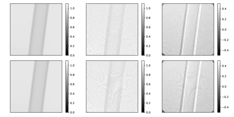
Figure 8: Transmission, visibility and phase images (from left to right) of the sample referenced to empty beam images. The top and bottom rows show results based on phase stepping curve evaluations with and without correction of the actual sampling positions respectively. The evaluation based on the assumption of error free sampling positions (bottom row) exhibits distinctive systematic errors modulated by the Moiré structure of the reference phase image.

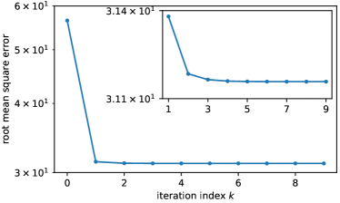
Figure 9: Root mean square error (RMSE) of the sinusoid fits to the phase stepping series throughout the iterations of Algorithm 1. After the first correction of the actual sampling locations by Eq. 16, the error is reduced by almost a factor of two. The following iterations further reduce the error confirming the validity of Alg. 1 for the solution of Eq. 5. Additional consideration of spatially inhomogeneous stepping distances (Eq. 2) further reduces the RMSE by merely 0.1%.

In addition to the mean deviations of the phase steps from the intended positions, spatial gradients throughout the detection area have been also considered (cf. Alg. 2). Figure 10 shows the respective differential deviations from the intended phase steps between the first 9 frames of the phase stepping series, normalized to the nominal homogeneous phase stepping increment of $2\pi/5$. The mean contributions of each component are listed in Table 1. While the homogeneous error of $0.1\,\text{rad}$ ranges within $10\%$ of the nominal step size (or $2\%$ of the grating period), the remaining effects are two to three orders of magnitude smaller. The root mean square error of the sinusoid fits for the whole phase stepping series is reduced by 0.1% relative to the optimization considering only homogeneous phase step deviations as shown in Figure 9. Consequently, the derived images (not shown) are visually equivalent to those obtained previously (cf. Fig. 8).

Figure 11 shows variations in the relative alignment of the gratings derived from the inhomogeneous phase stepping analysis by means of Equations 20–24. Besides deviations from the nominal linear motion of the gratings, minute rotations as well as subtle changes in relative magnification can also be detected. The correlation between grating rotations and translational errors visible in the left hand side graph in Figure 11 indicate rotations about an off-center pivot point about $10^{-1}\text{m}$ below the grating center, which is consistent with the actual placement of the phase stepping actuator in the experimental setup. Although the analog correlation between tilts about the horizontal axis and translation (along the optical axis) induced variations in magnification is much less pronounced (Fig. 11, right hand side), the mean trend and magnitude are also consistent with the assumption of a pivot point below the field of view. However, the observed magnitude ($10^{-7}$) of the relative mismatch of the effective grating periods is as well explicable by temperature variations in the order of magnitude of $10^{-1}\text{K}$ given a thermal expansion coefficient in the order of magnitude of $10^{-6}\text{K}^{-1}$ for the typical wafer materials silicon and graphite. Finally, the phase stepping inhomogeneities further suggest rotational motions about the vertical axis on the microrad scale (also shown in Fig. 11).

As a crude error assessment, the standard error of the mean phase deviation can be estimated from the sinusoid fits’ root mean square error:

$$\sigma_{\mathrm{mean}} \approx\frac{1}{\sqrt{\text{contributing detector pixels}}}\,\frac{\text{sinusoid fit RMSE}}{\text{mean sinusoid amplitude}}$$ (25)

$$\approx\sqrt{\frac{2}{\text{detector pixels}}}\,\frac{\text{sinusoid fit RMSE}}{\text{mean sinusoid amplitude}}\,.$$

The latter corresponds for the present data set to about $6\%$ of the mean observed sinusoid amplitude, which directly translates to $6\times 10^{-2}\,\text{rad}$ on the abscissa. Given the amount of detector pixels contributing to the least squares fits of $\Delta\phi_{i}(j)$ within each frame of the phase stepping series, a standard error in the order of magnitude of

$$\text{$\sigma_{\mathrm{mean}}$}\approx 10^{-4}\,\text{rad}$$ (26)

results. This implies that, according to the results given in Table 1, the tilt and slant contributions $\nabla_{\!hv}\phi$ and $\nabla_{\!h}^{2}\phi$ are close to the expected noise level for the present case.

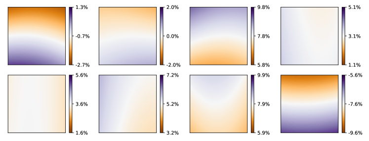
Figure 10: Relative deviations of the actual phase steps from the intended step width of $\frac{2\pi}{5}$ between the first nine frames of the phase stepping series ($\frac{5}{2\pi}(\Delta\phi_{i+1}(j)-\Delta\phi_{i}(j)-\frac{2\pi}{5})$). The variations $\Delta\phi_{i}(j)$ have been determined by optimization of Eq. 17 assuming the spatial dependence defined by Eq. 18 (see also Algorithm 2)

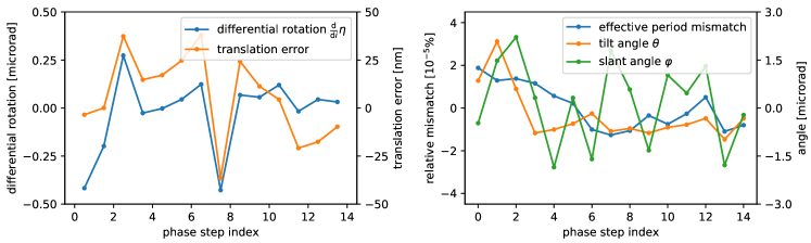
Figure 11: Quantitative results derivable from the inhomogeneities in the phase stepping deviations $\Delta\phi_{i}(j)$ (Eq. 18). On the left, the change in tilt angle about the optical axis from frame to frame within the phase stepping series is shown along with the accompanying linear motion error. Rotation correlated translations indicate an off-center pivot point. On the right hand side, the relative grating scaling error is shown along with the found tilt and slant about the horizontal and vertical axis. These quantities represent deviations from the mean grating alignment throughout the phase stepping series. The tilt and slant angles range close to the expected noise level (cf. Table 1 and Eq. 26).

4 Discussion and Conclusion

A fast converging iterative algorithm for the joint optimization of both the sinusoid model parameters and the actual sampling locations for the evaluation of grating interferometric phase stepping series has been proposed. Within the optimization procedure, spatially varying phase stepping increments due to further mechanical degrees of freedom besides the intended translatory stepping motion can also be accounted for. Mean phase stepping errors of up to 10% of the nominal step width have been found for a typical data set, and their correction results both in a considerable reduction of the overall root mean square error by almost a factor of two as well as a significant visual improvement of the final images. Although higher order effects are observable, their contribution was found to be two to three orders of magnitude smaller than that of the mean stepping error, and their correction thus did not contribute to further improvements in visual image quality in the present case. However, the higher order deviations allow the detection of minute motions of the gratings and thus provide a valuable tool for the monitoring and debugging of experimental setups. First order approximations for the relations between spatial phase variations and mechanical degrees of freedom of the moved grating have been given. For the present data set, linear motion errors up to $25\,\text{nm}$ as well as rotational motions on the microrad scale have been inferred from the phase stepping series. While the tilt and slant angles about the horizontal and vertical axes respectively have been found to range close to the expected noise level and should rather be interpreted as upper limits to actual motions, magnification changes in the range of $10^{-7}$ and sub-microrad rotations about the optical axis were well detectable. The expected correlations between rotation and translation due to an off-center pivot point further support the plausibility of the results. Especially the crosstalk between sub-microrad rotations and effective translations indicates that noticeable phase stepping errors will be almost inevitable even for very carefully designed experiments, wherefore an optimization based evaluation of the phase stepping series as proposed in Algorithm 1 is generally advisable. With processing speeds in the range of $0.1\,\text{s}$ per phase stepping series, it is well suitable as a standard processing method also for large image series.

References

- [1] C. David, B. Nöhammer, H. H. Solak, E. Ziegler: Differential x-ray phase contrast imaging using a shearing interferometer. Appl. Phys. Lett. 81 (17) 3287–3289 (2002). doi: 10.1063/1.1516611
- [2] Atsushi Momose, Shinya Kawamoto , Ichiro Koyama, Yoshitaka Hamaishi , Kengo Takai and Yoshio Suzuki: Demonstration of X-Ray Talbot Interferometry. Jpn. J. Appl. Phys. Vol. 42 (2003) pp. L 866–L 868
- [3] F. Pfeiffer, T. Weitkamp, O. Bunk, C. David: Phase retrieval and differential phase-contrast imaging with low-brilliance X-ray sources. Nature physics, 2(4), 258–261 (2006), doi:10.1038/nphys2
- [4] V. Revol, C. Kottler, R. Kaufmann, U. Straumann, C. Urban: Noise analysis of grating-based x-ray differential phase contrast imaging. Rev. Sci. Instrum. 81, 073709 (2010), doi:10.1063/1.3465334
- [5] M. Seifert, S. Kaeppler, C. Hauke, F. Horn, G. Pelzer, J. Rieger, T. Michel, C. Riess, G. Anton: Optimisation of image reconstruction for phase-contrast x-ray Talbot–Lau imaging with regard to mechanical robustness. Phys. Med. Biol. 61, 6441 (2016), doi:10.1088/0031-9155/61/17/6441
- [6] J. Vargas, C.O.S. Sorzano, J.C. Estrada, J.M. Carazo: Generalization of the Principal Component Analysis algorithm for interferometry. Opt. Comm. 286, 130–134 (2013)