Stress anisotropy in shear-jammed packings of frictionless disks

Abstract

We perform computational studies of repulsive, frictionless disks to investigate the development of stress anisotropy in mechanically stable (MS) packings. We focus on two protocols for generating MS packings: 1) isotropic compression and 2) applied simple or pure shear strain $\gamma$ at fixed packing fraction $\phi$. MS packings of frictionless disks occur as geometric families (i.e. parabolic segments with positive curvature) in the $\phi$-$\gamma$ plane. MS packings from protocol 1 populate parabolic segments with both signs of the slope, $d\phi/d\gamma>0$ and $d\phi/d\gamma<0$. In contrast, MS packings from protocol 2 populate segments with $d\phi/d\gamma<0$ only. For both simple and pure shear, we derive a relationship between the stress anisotropy and dilatancy $d\phi/d\gamma$ obeyed by MS packings along geometrical families. We show that for MS packings prepared using isotropic compression, the stress anisotropy distribution is Gaussian centered at zero with a standard deviation that decreases with increasing system size. For shear jammed MS packings, the stress anisotropy distribution is a convolution of Weibull distributions that depend on strain, which has a nonzero average and standard deviation in the large-system limit. We also develop a framework to calculate the stress anisotropy distribution for packings generated via protocol 2 in terms of the stress anisotropy distribution for packings generated via protocol 1. These results emphasize that for repulsive frictionless disks, different packing-generation protocols give rise to different MS packing probabilities, which lead to differences in macroscopic properties of MS packings.

I Introduction

For systems in thermal equilibrium, such as atomic and molecular liquids, macroscopic quantities, such as the shear stress and pressure, can be calculated by averaging over the microstates of the system weighted by the probabilities for which they occur, as determined by Boltzmann statistics McQuarrie (2000). In contrast, granular materials, foams, emulsions, and other athermal particulate media are out of thermal equilibrium and this formalism breaks down Jaeger et al. (1996); Baule et al. (2018).

For dense, quasistatically driven particulate media, the relevant microstates are mechanically stable (MS) packings with force- and torque-balance on all grains Gao et al. (2006); Shen et al. (2014). In contrast to thermal systems, the probabilities with which MS packings occur are highly non-uniform and depend on the protocol that was used to generate them Gao et al. (2009). For example, it has been shown that MS packings generated via vibration, compression, and pure and simple shear possess different average structural and mechanical properties Majmudar and Behringer (2005); Bi et al. (2011); Bertrand et al. (2016). In previous work on jammed packings of purely repulsive frictionless disks, we showed that the differences in macroscopic properties do not occur because the collections of microstates for each protocol are fundamentally different, instead the probabilities with which different MS packings occur change significantly with the protocol Bertrand et al. (2016). Thus, it is of fundamental importance to understand the relationship between the packing-generation protocol and MS packing probabilities.

Jamming, where an athermal particulate system transitions from a liquid-like to a solid-like state with a non-zero yield stress, induced by isotropic compression has been studied in granular and other athermal materials for more than 20 years Majmudar and Behringer (2005); Clusel et al. (2009); O’Hern et al. (2003). Recently, Bi, et al. showed that packings of granular disks can jam via simple and pure shear at fixed area Bi et al. (2011). This was a surprising result because many previous studies had emphasized that the application of shear at fixed packing fraction gives rise only to flow and unjamming behavior. This point is emphasized in the schematic jamming phase diagram in the stress $\Sigma$ and packing fraction $\phi$ plane in Fig. 1 (a), which shows that the yield stress $\Sigma^{y}$ or strain $\gamma^{y}$ increases with $\phi$ above jamming onset $\phi_{J}$ at zero shear. Here, we assume that $\Sigma^{y}\sim\gamma^{y}\sim(\phi-\phi_{J})^{\nu}$, where $\nu=0.5$. In Fig. 1 (b), we flip the axes so that the packing fraction at the yield strain increases quadratically from $\phi_{J}$ with increasing strain. In this picture, increasing the shear strain does not give rise to jamming. However, we will show below that this picture is incomplete, and the application of shear strain can cause unjammed systems of frictionless, spherical particles to jam Bertrand et al. (2016); Kumar and Luding (2016).

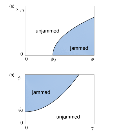
Figure 1: (a) A schematic jamming phase diagram in the stress $\Sigma$ and packing fraction $\phi$ plane. The solid line indicates the yield stress $\Sigma^{y}(\phi)$. For applied stress $\Sigma<\Sigma^{y}$, the system is jammed and for $\Sigma>\Sigma^{y}$, the system flows and is unjammed. We assume that the yield strain $\gamma^{y}$ scales with the yield stress and obeys $\Sigma^{y}\sim\gamma^{y}\sim(\phi-\phi_{J})^{\nu}$, where $\nu=0.5$ and $\phi_{J}$ is the jammed packing fraction in the absence of shear stress. (b) The same jamming phase diagram in (a) except rendered in the $\phi$-$\gamma$ plane. The jammed packing fraction increases quadratically with strain from $\phi_{J}$. With the phase diagrams in (a) and (b), increasing strain does not cause a system to transition from unjammed to jammed.

Despite important work Baity-Jesi et al. (2017); Bertrand et al. (2016); Kumar and Luding (2016) since the original manuscript by Bi, et al., there are still many open questions concerning shear jamming. For example, 1) Can shear jamming occur in MS packings of frictionless grains and if so, do these shear-jammed packings possess a nonzero stress anisotropy? and 2) Are there substantive differences between MS packings generated via isotropic compression versus shear?

Our recent work has shown that mechanically stable packings of frictionless spherical particles can be obtained via either simple shear or isotropic compression and that the probability for a particular packing depends on the packing-generation protocol Bertrand et al. (2016). The average shear strain required to jam an originally unjammed configuration can be written in terms of the basin volume, density of jammed packings, and path in configuration space from the initial condition to the final MS packing. This previous work focused mainly on the shear strain $\gamma_{J}$ needed to jam an initially unjammed configuration and how the shear strain $\gamma_{J}$ depends on the packing fraction. In the current article, we instead focus on the shear stress anisotropy in MS packings generated by isotropic compression versus pure and simple shear.

Our computational studies yield several key results, which form a more complete picture of shear jamming in packings of frictionless spherical particles. First, we identify relationships between the stress anisotropy and the packing fraction and its derivative with respect to strain (dilatancy) for MS packings generated via simple and pure shear. These relationships allow us to calculate the stress anisotropy (which includes contributions from both the shear stress and normal stress difference) for MS packings by only knowing how the jammed packing fraction varies with strain. Second, we show that the distribution of the stress anisotropy for isotropically compressed packings is a Gaussian centered on zero with a width that decreases as a power-law with increasing system size $N$ Xu and O’Hern (2006). In contrast, the stress anisotropy distribution is a convolution of strain-dependent Weibull distributions with a finite average and standard deviation in the large-system limit for shear-jammed MS packings Clark et al. (2015). Fourth, using the relation between stress anisotropy and dilatancy, we predict the stress anisotropy distribution for shear-jammed packings using that for MS packings generated via isotropic compression.

The remainder of the article includes three sections and three appendices, which provide additional details to support the conclusions in the main text. In Sec. II, we describe the two main protocols that we use to generate MS packings and provide definitions of the stress tensor and stress anisotropy. Sec. III includes four subsections that introduce the concept of geometrical families, derive the relationships between the stress tensor components and the dilatancy, develop a framework for calculating the shear stress distribution for shear-jammed packings in terms of the shear stress distribution for isotropically compressed packings, and describe the robustness of our results are with increasing system size. In Sec. IV, we give our conclusions, as well as describe interesting future computational studies on shear-jammed packings of non-spherical particles, such as circulo-polygons VanderWerf et al. (2018), and frictional particles Shen et al. (2014).

II Methods

Our computational studies focus on systems in two spatial dimensions containing $N$ frictionless bidisperse disks that interact via the purely repulsive linear spring potential given by $V(r_{ij})=\frac{\epsilon}{2}(1-r_{ij}/\sigma_{ij})^{2}\Theta(1-r_{ij}/\sigma_{ij})$, where $\epsilon$ is the strength of the repulsive interactions, $r_{ij}$ is the separation between the centers of disks $i$ and $j$, $\sigma_{ij}=(\sigma_{i}+\sigma_{j})/2$, $\sigma_{i}$ is the diameter of disk $i$, and $\Theta(.)$ is the Heaviside step function that prevents non-overlapping particles from interacting. The system includes half large disks and half small disks with diameter ratio $r=1.4$. The disks are confined within an undeformed square simulation cell with side lengths, $L_{x}=L_{y}=1$, in the $x$- and $y$-directions, respectively, and periodic boundary conditions. Isotropic compression is implemented by changing the cell lengths according to $L_{x}^{\prime}=L_{x}(1-d\phi/2\phi)$ and $L_{y}^{\prime}=Ly(1-d\phi/2\phi)$ and corresponding affine shifts in the particle positions, where $d\phi<10^{-4}$ is the change in packing fraction. Simple shear strain with amplitude $\gamma$ is implemented using Lees-Edwards periodic boundary conditions, where the top (bottom) images of the central cell are shifted to the right (left) by $\gamma L_{y}$ with corresponding affine shifts of the particle positions Lees and Edwards (1972). Pure shear is implemented by compressing the simulation cell along the $y$-direction and expanding it along the $x$-direction with corresponding affine shifts of the particle positions. The system area is kept constant (i.e. $A=L_{x}^{\prime}L_{y}^{\prime}=L_{x}L_{y}$) and the pure shear strain is defined as $\gamma=\ln(L_{x}^{\prime}/L_{y}^{\prime})$.

As shown in Fig. 2, we employ two main protocols to generate MS packings in the packing fraction $\phi$ and shear strain $\gamma$ plane. For protocol $1$, we first place the disks at random initial positions in the simulation cell, and apply successive simple shear strain steps $d\gamma<10^{-4}$ to total strain $\gamma_{t}$ at fixed small packing fraction $\phi_{i}=0.1$. We then isotropically compress the system in small packing fraction increments $d\phi$ to jamming onset $\phi_{J}$ at fixed simple shear strain $\gamma=\gamma_{t}$. For protocol 2, we first place the disks at random initial positions and then isotropically compress the system to a target packing fraction $\phi_{t}<\phi_{J}$ at simple shear strain $\gamma_{i}=0$. We then apply simple shear to the system in small strain steps $d\gamma$ until the system jams at $\gamma_{J}$. For protocol 2, the target volume fraction $\phi_{t}$ varies from $\phi_{m}$, below which no shear-jammed packings can be found in the range $0<\gamma<1$ to $\phi_{J}$ obtained from isotropic compression at $\gamma=0$. In Appendix A, we also include results for a packing-generation protocol similar to protocol 2, except we apply pure instead of simple shear strain.

The total potential energy per particle $U=U^{\prime}/N\epsilon$, where $U^{\prime}=\sum_{i>j}V(r_{ij})$, is minimized using the conjugate gradient technique after each compression or shear step. Minimization is terminated when the potential energy difference between successive conjugate gradient steps satisfies $\Delta U/U<10^{-16}$. We define jamming onset when the total potential energy per particle obeys $U_{\rm max}<U<2U_{\rm max}$, with $U_{\rm max}=10^{-16}$. This method for identifying jamming onset is similar to that used in our previous studies Bertrand et al. (2016).

The systems are decompressed (for protocol 1) or sheared in the negative strain direction (for protocol 2) when $U$ at a local minimum is nonzero, i.e., there are finite particle overlaps. If the potential energy is “zero” (i.e. $U<10^{-16}$), the system is compressed (for protocol 1) or sheared in the positive strain direction (for protocol 2). For protocol 1, the increment by which the packing fraction is changed at each compression or decompression step is halved each time $U$ switches from zero to nonzero or vice versa. Similarly, for protocol 2, the increment by which the shear strain is changed at each strain step is halved each time $U$ switches from zero to nonzero or vice versa. These packing-generation protocols yield mechanically stable packings (with a full-spectrum of nonzero frequencies of the dynamical matrix Tanguy et al. (2002)) at jamming onset. In addition, all of the MS disk packings generated via protocols 1 and 2 are isostatic, where the number of contacts matches the number of degrees of freedom, $N_{c}=N_{c}^{0}$, with $N_{c}^{0}=2N^{\prime}-1$, $N^{\prime}=N-N_{r}$, and $N_{r}$ is the number of rattler disks with fewer than three contacts Tkachenko and Witten (1999).

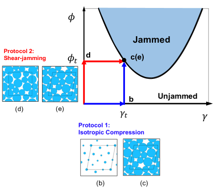
Figure 2: Schematic of the packing fraction $\phi$ and simple shear strain $\gamma$ plane that illustrates the two main protocols used to generate MS disk packings. As shown in Fig. 3 (e), the jammed regions are bounded by parabolic segments. In protocol 1, the system is first deformed to simple shear strain $\gamma_{t}$ at small initial packing fraction $\phi_{i}\approx 0$ (point b) and then isotropically compressed to jamming onset at $\phi_{t}$ (point c). In protocol 2, the system is first compressed to $\phi_{t}$ below jamming onset (point d) at $\gamma_{i}=0$ and then sheared to jamming onset at simple shear strain $\gamma_{t}$ (point e). Points (c) and (e) correspond to the same total deformation, and thus the two protocols can yield the same MS packing. Note that for each system size $N$, there are many distinct parabolas that occur over a range of strain and packing fraction. As the system size increases, the typical parabolic segment size decreases as $1/N$ and the range of packing fraction over which the parabolic segments occur shrinks to zero.

For each MS packing, we calculate the stress tensor:

$$\Sigma_{\beta\delta}=\frac{1}{A}\sum_{i\neq j}f_{ij\beta}r_{ij\delta},$$ (1)

where $A=L_{x}L_{y}$ is the system area, $f_{ij\beta}$ is the $\beta$-component of the interparticle force on particle $i$ due to particle $j$, $r_{ij\delta}$ is the $\delta$-component of the separation vector from the center of particle $j$ to that of particle $i$, and $\beta$ and $\delta=x$,$y$. From the components of the stress tensor, we can calculate the pressure $P=(\Sigma_{xx}+\Sigma_{yy})/2$, the normal stress difference $\Sigma_{N}=(\Sigma_{yy}-\Sigma_{xx})/2$, and the shear stress $-\Sigma_{xy}$. We define the normalized stress anisotropy to be $\hat{\tau}=\sqrt{\hat{\Sigma}_{N}^{2}+\hat{\Sigma}_{xy}^{2}}$, where $\hat{\Sigma}_{N}=\Sigma_{N}/P$ and $\hat{\Sigma}_{xy}=-\Sigma_{xy}/P$. $\hat{\tau}$ includes contributions from both the shear stress and the normal stress difference. We will show below that only the shear stress (normal stress difference) contributes to $\hat{\tau}$ for MS packings generated via simple shear (pure shear). Therefore, we will focus on $\hat{\Sigma}_{xy}$ when we study packings generated via simple shear and on $\hat{\Sigma}_{N}$ when we study packings generated via pure shear. (See Appendix A.) We calculate mean values and standard deviations of the stress tensor components over between $10^{3}$ and $10^{5}$ distinct MS packings.

III Results

III.1 Geometrical families

As background, we review the structure of geometrical families during shear deformation Gao et al. (2009); Bertrand et al. (2016). In Fig. 3 (a), we illustrate that MS packings occur as geometrical families, forming continuous segments in the jammed packing fraction $\phi$ and shear strain $\gamma$ plane, with the same interparticle contact networks. In panel (a), the $N=6$ MS packings were generated using isotropic compression (protocol 1) from a single random initial condition. In Fig. 3 (c) and (d), we highlight two MS packings near the beginning and end of the geometrical family indicated by the filled triangles in (a). The system switches from one geometrical family to another when the interparticle contact network becomes unstable. The beginning and end of each geometrical family can be identified by finding changes in the interparticle contact network or discontinuous changes in $\phi(\gamma)$ or slope $d\phi/d\gamma$.

Each geometrical family of MS packings forms a parabolic segment in the $\phi$-$\gamma$ plane described by $\phi(\gamma)=A(\gamma-\gamma_{0})^{2}+\phi_{0}$, where $A$, $\gamma_{0}$, and $\phi_{0}$ give the curvature, strain offset, and packing fraction offset for each family. The curvature satisfies $A>0$ for all geometrical families of MS disk packings. In Fig. 3 (e) and (f), we show that the data collapse onto a parabolic form when we plot $(\phi-\phi_{0})/A$ versus $\gamma-\gamma_{0}$ for all geometric families we found using protocols 1 and 2, respectively, with more than $10^{5}$ initial conditions. For protocol 1, we obtain families with both $d\phi/d\gamma>0$ and $d\phi/d\gamma<0$. However, for protocol 2, the geometrical families only possess $d\phi/d\gamma<0$. For protocol 1, the systems approach the jammed region from below, and thus they can reach both sides of the parabolas. For protocol 2, the systems approach the jammed region from the left, and thus they jam when they reach the left sides of the parabolas. Note the key difference in the signs of the slope, $d\phi/d\gamma$, between the jamming phase diagrams in Figs. 1 (b) and 3 (f). The schematic jamming phase diagram in Fig. 1 (b) is missing the portion of the parabola with $d\phi/d\gamma<0$.

The geometrical family structure can also be seen in the shear stress versus strain as shown in Fig. 3 (b). In this case, the shear stress $|{\hat{\Sigma}}_{xy}|$ varies quasi-linearly with $\gamma$. For MS packings within a given geometrical family, we find that $|\hat{\Sigma}_{xy}|$ increases with $\phi$ and $|\hat{\Sigma}_{xy}|\approx 0$ when $\phi(\gamma)$ is near a local minimum or maximum (i.e., $\frac{\partial\phi}{\partial\gamma}=0$). Although we illustrated these results for a small system, we showed in previous studies Bertrand et al. (2016) that the geometrical family structure persists with increasing system size. In large-system limit, the family structure occurs over a narrow range of $\phi$ near $\phi_{J}\approx 0.84$, and the system only needs to be sheared by an infinitesimal strain to switch from one family to another.

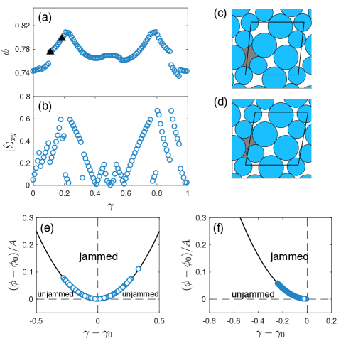
Figure 3: (a) Packing fraction $\phi$ at jamming onset as a function of simple shear strain $\gamma$ for MS packings with $N=6$ generated via isotropic compression (protocol 1) and (b) the corresponding magnitude of the shear stress $\left|\hat{\Sigma}_{xy}\right|$ versus $\gamma$. The data in (a) and (b) were obtained using the same single set of random initial conditions. Panels (c) and (d) show the MS packings near the start and the end of a geometrical family, indicated by the lower and upper filled triangles in (a). Each geometrical family in (a), as well as the families obtained from other random initial conditions, can be described by parabolic segments, $\phi=A(\gamma-\gamma_{0})^{2}+\phi_{0}$, in the $\phi$-$\gamma$ plane, where $A>0$, $\phi_{0}$, and $\gamma_{0}$ are the curvature, packing fraction offset, and strain offset for each geometrical family. Panels (e) and (f) show the normalized coordinates, $(\phi-\phi_{0})/A$ versus $\gamma-\gamma_{0}$, for all MS packings with $N=6$ generated via protocols 1 and 2, respectively. Protocol 1 generates packings with both signs of $d\phi/d\gamma$, whereas protocol 2 only generates packings with $d\phi/d\gamma<0$. The jammed and unjammed regions of the $(\phi-\phi_{0})/A$ and $\gamma-\gamma_{0}$ plane are indicated.

III.2 Relationship between the stress tensor components and dilatancy

In this section, we derive relationships between the components of the stress tensor (i.e. the shear stress ${\hat{\Sigma}}_{xy}$ and normal stress difference ${\hat{\Sigma}}_{N}$) and the packing fraction and dilatancy Peyneau and Roux (2008); Kabla and Senden (2009); Kruyt and Rothenburg (2006), $d\phi/d\gamma$, for MS packings generated via protocols 1 and 2. For MS packings belonging to a given geometrical family, the total energy does not change following a strain step $d\gamma$ and a decompression step that changes the area by $dA$. Thus, the total work is given by $-PdA-\Sigma_{xy}Ad\gamma=0$ for simple shear and $-PdA-\Sigma_{yy}L_{x}^{\prime}dL_{y}^{\prime}-\Sigma_{xx}L_{y}^{\prime}dL_{x}^{\prime}=0$ for pure shear. Using $dA/A=-d\phi/\phi$, we find

$${\hat{\Sigma}}=-\frac{1}{\phi}\frac{d\phi}{d\gamma},$$ (2)

where ${\hat{\Sigma}}={\hat{\Sigma}}_{xy}$ for simple shear and ${\hat{\Sigma}}_{N}$ for pure shear deformations. Thus, the shear stress $\hat{\Sigma}_{xy}$ (normal stress difference $\hat{\Sigma}_{N}$) along a geometrical family is proportional to the dilatancy, $d\phi/d\gamma$, during simple (pure) shear deformation.

In Fig. 4 (a) and (b), we compare the results from the calculations of the shear stress and normal stress difference using the stress tensor (Eq. 1) to those using Eq. 2 for $N=6$ MS packings generated using protocol 1. We find strong agreement. In Fig. 4 (c) and (d), we further compare the two methods for calculating the stress tensor components by plotting ${\hat{\Sigma}}_{xy}$ or ${\hat{\Sigma}_{N}}$ from the stress tensor versus the right side of Eq. 2 for several system sizes and protocols 1 and 2. The data collapse onto a line with unit slope and zero vertical intercept. Data points that deviate from the straight line collapse onto the line when $d\gamma$ is decreased to $2\times 10^{-4}$.

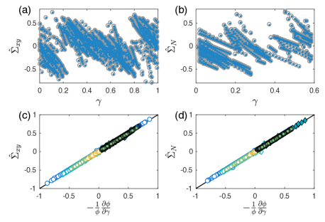
Figure 4: (a) Shear stress $\hat{\Sigma}_{xy}$ versus simple shear strain $\gamma$ and (b) normal stress difference $\hat{\Sigma}_{N}$ versus pure shear strain $\gamma$ for $N=6$ MS packings generated via isotropic compression (protocol 1). Gray circles are data points obtained from the components of the stress tensor and blue dots are obtained by finding all of the geometrical families and calculating $\hat{\Sigma}_{xy}$ and $\hat{\Sigma}_{N}$ from Eq. 2 along each family. Panels (c) and (d) show plots of $\hat{\Sigma}_{xy}$ and $\hat{\Sigma}_{N}$ calculated using the stress tensor versus the results from Eq. 2 for MS packings with $N=6$ (circles), $10$ (diamond), $16$ (squares), and $32$ (upward triangles). Open (solid) symbols indicate MS packings generated via protocol 1 (protocol 2). The solid line has unit slope and zero vertical intercept.

III.3 Distributions of the shear stress and normal stress difference for protocols 1 and 2

In the inset of Fig. 5 (a), we show the probability distributions for the shear stress and normal stress difference, $P(\hat{\Sigma}_{xy})$ and $P(\hat{\Sigma}_{N})$, for MS packings generated via isotropic compression (protocol 1) and $P(\hat{\Sigma}_{N})$ for MS packings generated via protocol 2 with simple shear. When scaled by the standard deviation $S$, these distributions collapse onto a Gaussian curve centered at zero with unit standard deviation. As shown in Fig. 5 (b), the standard deviations for all three distributions scale with system size as

$$S_{1}(N)=S^{0}_{1}N^{-\omega_{1}},$$ (3)

where $S^{0}_{1}\approx 0.61$ and $\omega_{1}\approx 0.48$. Thus, the stress tensor is isotropic in the large system-limit for MS packings generated via isotropic compression (protocol 1). In addition, the normal stress difference is zero for MS packings generated via protocol 2 with simple shear.

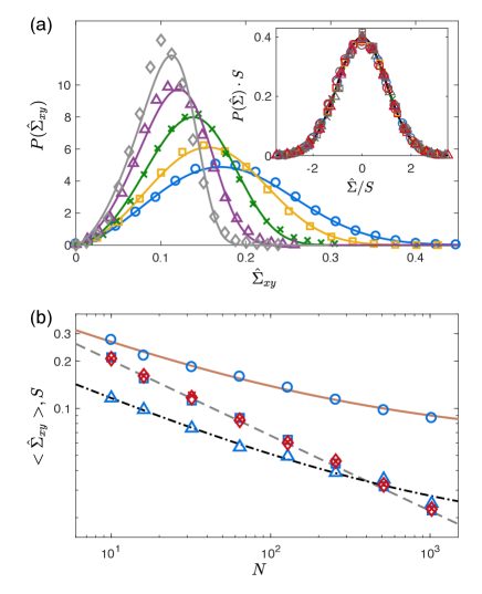
Figure 5: (a) The probability distributions of the shear stress $P(\hat{\Sigma}_{xy})$ for MS packings generated via protocol 2 with simple shear for $N=32$ (circles), $64$ (squares), $128$ (crosses), $256$ (triangles), and $512$ (diamonds). The solid lines are predictions from Eq. 13. In the inset, we show three types of probability distributions scaled by their standard deviations $S$: $P(\hat{\Sigma}_{xy})$ (same symbols as main panel) and $P({\hat{\Sigma}}_{N})$ (same symbols as main panel, but in red) for MS packings generated via isotropic compression (protocol 1) and $P({\hat{\Sigma}}_{N})$ for protocol 2 with simple shear (same symbols as main panel, but in gray). The solid black line is a Gaussian distribution with zero mean and unit standard deviation. (b) System-size dependence of $\langle\hat{\Sigma}_{xy}\rangle$ (circles) and standard deviations of $P(\hat{\Sigma}_{xy})$ (triangles) and $P(\hat{\Sigma}_{N})$ (squares) for MS packings generated via protocol 2 with simple shear and the standard deviations of $P(\hat{\Sigma}_{xy})$ (crosses) and $P(\hat{\Sigma}_{N})$ (diamonds) for MS packings generated via protocol 1. The dashed, solid, and dash-dotted lines are fits to Eqs. 3, 4, and 5, respectively.

Table 1: Means ($\langle.\rangle$) and standard deviations ($S$) of the shear stress ${\hat{\Sigma}}_{xy}$ and normal stress difference ${\hat{\Sigma}}_{N}$ distributions in the large-system limit for protocols 1 and 2.

Protocol	$\langle\hat{\Sigma}_{xy}\rangle_{\infty}$	$\langle\hat{\Sigma}_{N}\rangle_{\infty}$	$S^{xy}_{\infty}$	$S^{N}_{\infty}$
Protocol 1	0	0	0	0
Protocol 2
simple shear	0.060	0	0.015	0
protocol 2
pure shear	0	0.055	0	0.016

In the main panel of Fig. 5 (a), we show the probability distribution of the shear stress $P({\hat{\Sigma}}_{xy})$ for MS packings generated via protocol 2 with simple shear. We note that ${\hat{\Sigma}}_{xy}>0$ and $P({\hat{\Sigma}}_{xy})$ is non-Gaussian for protocol 2. In contrast to the behavior of the average shear stress $\langle{\hat{\Sigma}}_{xy}\rangle$ for MS packings generated via isotropic compression (protocol 1), $\langle\hat{\Sigma}_{xy}\rangle$ approaches a nonzero value in the large-system limit for MS packings generated via protocol 2 with simple shear. As shown in Fig. 5 (b),

$$\langle\hat{\Sigma}_{xy}\rangle(N)=\hat{\Sigma}_{0}N^{-\Omega}+\hat{\Sigma}_{\infty},$$ (4)

where $\hat{\Sigma}_{0}\approx 0.54$, $\Omega\approx 0.42$, and $\hat{\Sigma}_{\infty}\approx 0.060$. Similarly, we find that the standard deviation of $P({\hat{\Sigma}}_{xy})$ for MS packings generated via protocol 2 with simple shear approaches a nonzero value in the large-system limit:

$$S_{2}(N)=S_{2}^{0}N^{-\omega_{2}}+S_{\infty},$$ (5)

where $S_{2}^{0}\approx 0.28$, $\omega_{2}\approx 0.45$, and $S_{\infty}\approx 0.015$. In contrast, the width of the distribution of jammed packing fractions tends to zero in the large-system limit O’Hern et al. (2003). Thus, the packing-generation protocol strongly influences the stress anisotropy, especially in the large-system limit. The results for the average values and standard deviations of the distributions $P({\hat{\Sigma}}_{xy})$ and $P({\hat{\Sigma}}_{N})$ in the large-system limit for protocols 1 and 2 (for simple and pure shear) are summarized in Table 1.

The stress anisotropy measured here is smaller than the value obtained in other recent work (${\hat{\Sigma}}_{xy}\approx 0.095$) Zheng et al. (2018). The shear-jamming protocol in this prior work is very different than the one presented here. We isotropically compress the system to a packing fraction below jamming onset for each particular initial condition, and then apply quasistatic shear at fixed area until the system first jams at strain $\gamma_{J}$. In contrast, in these prior studies, the authors start with jammed packings at a given pressure $P>0$ and then apply quasistatic shear at fixed $P$ to a total strain $\gamma=10$. Thus, the system can undergo rearrangements and switch from one geometrical family to another. Moreover, these prior studies only quoted a stress anisotropy for a finite-sized system ($N=1024$), and did not provide an estimate for the stress anisotropy in the large system limit.

We will now describe a framework for determining the distribution of shear stress $P({\hat{\Sigma}}_{xy})$ for MS packings generated via protocol 2 with simple shear from the shear stress distribution obtained from protocol 1. We first make an approximation in Eq. 2, $\hat{\Sigma}_{xy}\approx-\frac{1}{\langle\phi\rangle_{2}}\frac{d\phi}{d\gamma}$, where $\langle\phi\rangle_{2}$ is the average packing fraction for MS packings generated using protocol 2. Now, the goal is to calculate the distribution of the dilatancy, which hereafter we define as $\dot{\phi}\equiv-\frac{d\phi}{d\gamma}$.

We first consider an infinitesimal segment of a geometrical family (labeled $i$) that starts at $(\gamma_{i},\phi_{i})$ and ends at $(\gamma_{i}+\mathrm{d}\gamma,\phi_{i}-\mathrm{d}\phi)$. We only need to consider segments with negative slope, which implies that $\mathrm{d}\gamma>0$, $\mathrm{d}\phi>0$, and $\dot{\phi}>0$. The probability to obtain an MS packing on segment $i$ is proportional to (1) the volume of the initial conditions in configuration space that find segment $i$ Xu et al. (2011); Ashwin et al. (2012), $V_{1,i}$ for protocol 1 and $V_{2,i}$ for protocol 2, and (2) the region of parameter space over which the segment is sampled, $d\gamma_{i}$ for protocol 1 and $d\phi_{i}$ for protocol 2. Thus, $P_{1,i}\propto V_{1,i}d\gamma_{i}$ for protocol 1 and $P_{2,i}\propto V_{2,i}d\phi_{i}$ for protocol 2.

The probability distribution for the dilatancy $\dot{\phi}$ can be written as:

$$P_{1,2}(\dot{\phi})=\frac{V_{1,2}(\dot{\phi})}{\int_{0}^{\infty}V_{1,2}(\dot{\phi})\mathrm{d}\dot{\phi}},$$ (6)

where $V_{1,2}(\dot{\phi})$ is the sum of the basin volumes over all of the infinitesimal segments with slope $\dot{\phi}$,

$$V_{1}(\dot{\phi}) =\sum_{i}V_{1,i}(\dot{\phi})\mathrm{d}\gamma_{i}$$ (7a)

$$V_{2}(\dot{\phi}) =\sum_{i}V_{2,i}(\dot{\phi})\mathrm{d}\phi_{i}.$$ (7b)

In the small-$\gamma$ limit ($\gamma_{i}\approx 0$), the basin volumes for each segment $i$ from protocols 1 and 2 satisfy $V_{1,i}\approx V_{2,i}$. (In Appendix B, we identify the shear strain at which this approximation breaks down.) In this limit, the protocol dependence of $P(\dot{\phi})$ is caused by the region of parameter space over which the MS packings are sampled, $d\gamma_{i}$ for protocol 1 versus $d\phi_{i}$ for protocol 2. Thus, the distribution of dilatancy for protocol 2 for simple shear is given by:

$$P_{2}(\dot{\phi}) =\frac{\sum_{i}V_{2,i}\mathrm{d}\phi_{i}}{\int_{0}^{\infty}\sum_{i}V_{2,i}\mathrm{d}\phi_{i}\mathrm{d}\dot{\phi}}\approx\frac{\sum_{i}V_{1,i}\mathrm{d}\gamma_{i}\dot{\phi}}{\int_{0}^{\infty}\sum_{i}V_{1,i}\mathrm{d}\gamma_{i}\dot{\phi}\mathrm{d}\dot{\phi}}$$ (8a)

$$\approx\frac{P_{1}(\dot{\phi})\dot{\phi}}{\langle\dot{\phi}\rangle_{1}},$$ (8b)

where we have used the relation $d\phi_{i}=d\gamma_{i}{\dot{\phi}}$ and $\langle\dot{\phi}\rangle_{1}$ is the average of $\dot{\phi}$ for MS packings generated using protocol 1 with $\dot{\phi}>0$.

In Fig. 5 (a), we show that the dilatancy distribution $P_{1}(\dot{\phi})$ for ${\dot{\phi}}>0$ from protocol 1 obeys a half-Gaussian distribution,

$$P_{1}(\dot{\phi})=\frac{\sqrt{2}}{S_{1}\sqrt{\pi}}\mathrm{exp}\left(-\frac{\dot{\phi}^{2}}{2S_{1}^{2}}\right),$$ (9)

with standard deviation $S_{1}$. After we substitute $P_{1}(\dot{\phi})$ given by Eq. 9 and $\langle\dot{\phi}\rangle_{1}=\sqrt{2/\pi}S_{1}$ into Eq. 8b, we find the following expression for the dilatancy distribution for MS packings generated via protocol 2 with simple shear in the small-$\gamma$ limit:

$$P_{2}(\dot{\phi}|\gamma\ll 1)=\frac{k_{0}}{\lambda_{0}}\left(\frac{\dot{\phi}}{\lambda_{0}}\right)^{k_{0}-1}\mathrm{exp}\left[-\left(\frac{\dot{\phi}}{\lambda_{0}}\right)^{k_{0}}\right].$$ (10)

$P_{2}({\dot{\phi}}|\gamma\ll 1)=f_{w}(\dot{\phi};\lambda_{0},k_{0})$ is a Weibull distribution with shape parameter $k_{0}=2$ and scale parameter $\lambda_{0}=\sqrt{2}S_{1}$. We show in Fig. 6 (b) that the prediction in Eq. 10 agrees quantitatively with the simulation results for $\gamma<2\times 10^{-4}$ over a range of system sizes.

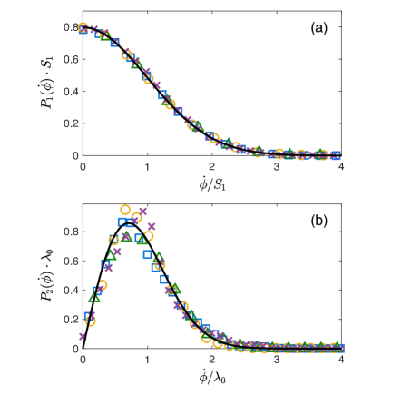
Figure 6: (a) Probability distribution of the dilatancy $P_{1}(\dot{\phi})$ for $\dot{\phi}>0$ scaled by the standard deviation $S_{1}$ for MS packings generated via protocol 1 with $N=64$ (squares), $128$ (circles), $256$ (triangles), and $512$ (crosses). The solid line is the half-Gaussian distribution in Eq. 9. (b) Probability distribution of the dilatancy $P(\dot{\phi})$ for MS packings generated via protocol 2 with simple shear in the small strain limit ($\gamma<2\times 10^{-4}$). The symbols are the same as in panel (a). The solid line is the Weibull distribution in Eq. 10 with shape parameter $k_{0}=2$ and scale parameter $\lambda_{0}=\sqrt{2}S_{1}$.

We will now consider the dilatancy distribution for MS packings generated via protocol 2 at finite shear strains. For protocol 1 (isotropic compression), our previous studies have shown that the distribution of jammed packing fractions is independent of the shear strain $\gamma$ Bertrand et al. (2016). However, for protocol 2 (e.g. with simple shear), systems will preferentially jam on geometrical families at small $\gamma$, effectively blocking families at larger $\gamma$, which causes the fraction of unjammed packings to decay exponentially with increasing $\gamma$ for protocol 2 at a given $\phi$ Bertrand et al. (2016). Therefore, as $\gamma$ increases, the assumption that $V_{1,i}\approx V_{2,i}$ is no longer valid, as shown in Appendix B. To characterize the $\gamma$-dependence of the dilatancy distribution, we partition the packings into regions of strain $\gamma$ required to jam them. We can then express the dilatancy distribution for MS packings generated via protocol 2 with simple shear as an integral over $\gamma$:

$$P_{2}(\dot{\phi})=\int_{0}^{\infty}P_{2}(\dot{\phi}|\gamma)P_{2}(\gamma)d\gamma,$$ (11)

where $P_{2}(\dot{\phi}|\gamma)$ is the conditional probability for obtaining $\dot{\phi}$ at a given $\gamma$ and $P_{2}(\gamma)$ is the probability for obtaining an MS packing as a function of $\gamma$, which displays exponential decay Bertrand et al. (2016): $P_{2}(\gamma)=\alpha\exp(-\alpha\gamma)$. We show in Fig. 7 (a) that $P_{2}(\dot{\phi}|\gamma)$ obeys a Weibull distribution, $f_{w}(\dot{\phi};\lambda,k)$, with shape $k(\gamma)$ and scale parameters $\lambda(\gamma)$ that depend on strain $\gamma$. $k(\gamma)$ and $\lambda(\gamma)$ decay exponentially to steady-state values in the large-$\gamma$ limit as shown in Fig. 7 (b):

$$\frac{\chi_{\infty}-\chi(\gamma)}{\chi_{\infty}-\chi_{0}}=\exp(-\gamma/\gamma_{c}),$$ (12)

where $\chi=k$, $\lambda$ and $\chi_{0}$ and $\chi_{\infty}$ are the values when $\gamma=0$ and $\gamma\rightarrow\infty$, respectively. We find that both $k$ and $\lambda$ reach steady-state values when $\gamma>\gamma_{c}$, where $\gamma_{c}\approx 0.02$ in the large-system limit.

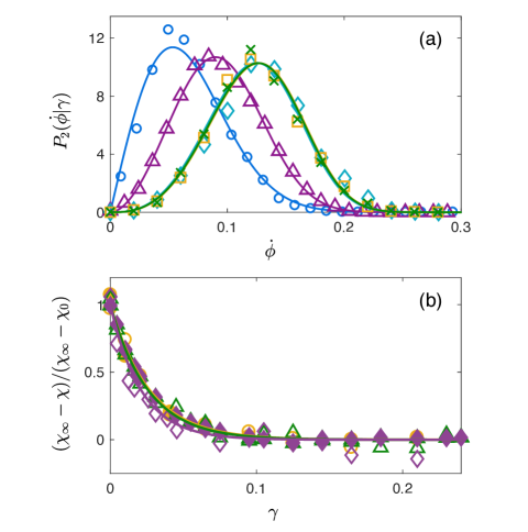
Figure 7: (a) The conditional probability $P_{2}(\dot{\phi}|\gamma)$ for obtaining dilatancy ${\dot{\phi}}$ for MS packings with $N=128$ generated via protocol 2 with simple shear for $\gamma<2\times 10^{-4}$ (circles), $0.012<\gamma<0.016$ (triangles), $0.20<\gamma<0.22$ (diamonds), $0.22<\gamma<0.24$ (squares), and $0.24<\gamma<0.26$ (crosses). The solid lines are Weibull distributions $f_{w}({\dot{\phi}},\lambda(\gamma),k(\gamma))$. (b) The $\gamma$-dependence of the shape parameter $\chi=k$ (open symbols) and scale parameter $\chi=\lambda$ (solid symbols) for fits of $P_{2}({\dot{\phi}}|\gamma)$ to Weibull distributions for $N=128$ (circles), $256$ (triangles), and $512$ (diamonds). $\chi_{0}$ and $\chi_{\infty}$ give the values of $k$ and $\lambda$ at $\gamma=0$ and in the $\gamma\rightarrow\infty$ limit, respectively. The solid lines are fits to an exponential decay, $\sim\exp(-\gamma/\gamma_{c})$, where $\gamma_{c}=0.027$, $0.026$, and $0.021$ for $N=128$, $256$, and $512$, respectively.

In the final step, we combine Eqs. 10 and 11 with the results from Eq. 12 to predict the distribution of shear stress for MS packings generated via protocol 2 with simple shear:

$$P_{2}(\hat{\Sigma}_{xy})=\langle\phi\rangle_{2}\int_{0}^{\infty}f_{w}({\dot{\phi}};\lambda(\gamma),k(\gamma))\alpha\exp\left(-\alpha\gamma\right)d\gamma,$$ (13)

where $\hat{\Sigma}_{xy}=\dot{\phi}/\langle\phi\rangle_{2}$ has been used to relate $P_{2}(\hat{\Sigma}_{xy})$ to $P_{2}(\dot{\phi})$. The results from Eq. 13 agree quantitatively with the distribution directly calculated from the stress tensor components over a range of system sizes as shown in Fig. 5 (a). Thus, these results emphasize that we are able to calculate the distribution of shear stress for MS packings generated via protocol 2 from the distribution of shear stress from MS packings generated via protocol 1, plus only three parameters: $\alpha\gamma_{c}$, $k_{\infty}$, and $\lambda_{\infty}$. We will show below that $\langle{\hat{\Sigma}}_{xy}\rangle$ depends very weakly on $k_{\infty}$.

III.4 System-size dependence of the average stress anisotropy for shear-jammed packings

In Fig. 5, we showed that the average shear stress $\langle{\hat{\Sigma}}_{xy}\rangle\sim 0.06$ reaches a nonzero value in the large-system limit for MS packings generated via protocol 2 with simple shear. In this section, we investigate the system size dependence of $\langle{\hat{\Sigma}}_{xy}\rangle$ using the framework (Eq. 13) for calculating the shear stress distribution for MS packings generated via protocol 2 using the shear stress distribution for MS packings generated via isotropic compression (protocol 1).

$\langle\hat{\Sigma}_{xy}\rangle$ for MS packings generated via protocol 2 can be calculated from the probability distribution $P_{2}({\hat{\Sigma}}_{xy})$:

$$\langle\hat{\Sigma}_{xy}\rangle =\int_{0}^{\infty}\hat{\Sigma}_{xy}P_{2}(\hat{\Sigma}_{xy})d\hat{\Sigma}_{xy}$$ (14)

$$\approx\int_{0}^{\infty}\frac{\dot{\phi}}{\langle\phi\rangle_{2}}(\langle\phi\rangle_{2}P_{2}(\dot{\phi}))\frac{\mathrm{d}\dot{\phi}}{\langle\phi\rangle_{2}}=\frac{1}{\langle\phi\rangle_{2}}\int_{0}^{\infty}\dot{\phi}P_{2}(\dot{\phi})\mathrm{d}\dot{\phi}.$$

After substituting Eq. 11 into Eq. 14, we have

$$\langle\hat{\Sigma}_{xy}\rangle =\frac{1}{\langle\phi\rangle_{2}}\int_{0}^{\infty}\dot{\phi}\left(\int_{0}^{\infty}f_{w}(\dot{\phi};\lambda(\gamma),k(\gamma))\alpha\exp\left(-\alpha\gamma\right)d\gamma\right)d\dot{\phi}$$ (15)

$$=\frac{1}{\langle\phi\rangle_{2}}\int_{0}^{\infty}\langle\dot{\phi}\rangle_{\gamma}\alpha\exp\left(-\alpha\gamma\right)d\gamma,$$

where $\langle\dot{\phi}\rangle_{\gamma}=\lambda(\gamma)\Gamma(1+1/k(\gamma))$ is the average of $\dot{\phi}$ at strain $\gamma$. The shape parameter $k(0)=2$ and increases with $\gamma$, and thus $0.886\lesssim\Gamma(1+1/k(\gamma))<1$. Therefore, $\langle\dot{\phi}\rangle_{\gamma}$ can be approximated as

$$\langle\dot{\phi}\rangle_{\gamma}\approx\lambda(\gamma)=\lambda_{\infty}[1-\exp(-\gamma/\gamma_{c})]+\lambda_{0}\exp(-\gamma/\gamma_{c}).$$ (16)

After substituting Eq. 16 into Eq. 15, we find

$$\langle\hat{\Sigma}_{xy}\rangle\approx\frac{\lambda_{\infty}+\lambda_{0}\alpha\gamma_{c}}{\langle\phi\rangle_{2}(\alpha\gamma_{c}+1)},$$ (17)

which is plotted versus system size in Fig. 8. We fit the system-size dependence to following form:

$$\langle{\hat{\Sigma}}_{xy}\rangle(N)={\hat{\Sigma}}_{0}N^{-\Omega}+{\hat{\Sigma}}_{\infty},$$ (18)

where ${\hat{\Sigma}}_{0}\approx 0.62$, $\Omega\approx 0.41$, and ${\hat{\Sigma}}_{\infty}\approx 0.060$, which are similar to the values found directly using the data in Fig. 5.

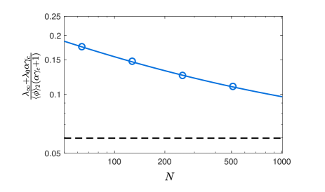
Figure 8: The system-size dependence of $\langle{\hat{\Sigma}}_{xy}\rangle\approx(\lambda_{\infty}+\lambda_{0}\alpha\gamma_{c})/[\langle\phi\rangle_{2}(\alpha\gamma_{c}+1)]$ (circles) from Eq. 17. The best fit to Eq. 18 is given by the solid line. The shear stress in the large-system limit $\langle{\hat{\Sigma}}_{xy}\rangle_{\infty}\approx 0.060$ is indicated by the dashed line.

IV Conclusions and Future Directions

In this article, we carried out computer simulations of frictionless, purely repulsive disks to investigate the development of stress anisotropy in mechanically stable (MS) packings prepared using two protocols. Protocol 1 involves shearing the system quasistatically to a given strain at low packing fraction and then compressing the system quasistatically to jamming onset at fixed strain. Protocol 2 involves compressing the system quasistatically at $\gamma=0$ to a packing fraction below jamming onset, and then shearing the system quasistatically to achieve jamming onset.

We find that the stress anisotropy distribution for MS packings generated via protocol 1 is a Gaussian with zero mean and a standard deviation that scales to zero in the large-system limit. In contrast, MS packings prepared using protocol 2 have a nonzero stress anisotropy ${\hat{\tau}}_{\infty}\approx 0.06$ and standard deviation $S_{\infty}\approx 0.015$ in the large-system limit. We also derived relationships between the components of the stress tensor (shear stress and normal stress difference) and the dilatancy $d\phi/d\gamma$. Using these relations, we developed a statistical framework to calculate the stress anisotropy distribution for shear-jammed packings (i.e. MS packings generated via protocol 2) in terms of the stress anisotropy distribution for isotropically prepared packings (i.e. MS packings generated via protocol 1). We showed that the stress anisotropy distribution for shear-jammed packings can be described by a convolution of Weibull distributions with shape and scale parameters that depend on strain. The results for the stress anisotropy distribution from the statistical framework agree quantitatively with the direct measurements of the stress tensor for MS packings generated using protocol 2. These results emphasize that the packing-generation protocol can dramatically influence the probabilities with which MS packings occur, and thus change the average macroscopic quantities that are measured for a given protocol.

There are several interesting directions for future research investigating the development of stress anisotropy in jammed systems. First, how does the presence of frictional interparticle forces affect this picture? Recent computational studies have shown that the shear modulus displays a discontinuous jump with increasing strain for static packings of frictional spheres Otsuki and Hayakawa (2017). Can the discontinuity in the shear modulus be explained using the statistical framework for the shear stress distribution that we developed here? Moreover, there are still open questions about whether pure/simple shear and isotropic compression can give rise to fundamentally different ensembles of MS packings of frictional particles. For example, consider the Cundall-Strack model for static friction between contacting grains Cundall and Strack (1979). In this model, the tangential force, which is proportional to the relative tangential displacement between contacting grains can grow until the ratio of the magnitude of the tangential to normal force reaches the static friction coefficient $\mu$. If the ratio exceeds $\mu$, the particle slips and the relative tangential displacement is reset. Two packings with identical particle positions can possess different numbers of near-slipping contacts. It is thus possible that different packing-generation protocols will lead to nearly identical MS packings with different numbers of near-slipping contacts.

Second, how does non-spherical particle shape affect the geometrical families $\phi(\gamma)$? In preliminary studies, we have shown that the geometrical families for MS packings of circulo-polygons occur as parabolic segments that are both concave up and concave down. (See Appendix C.) In future studies, we will generate packings of circulo-polygons using protocol 2 to connect the statistics of the geometrical families $\phi(\gamma)$ to the development of nonzero stress anisotropy in the large-system limit for MS packings of non-spherical particles.

Appendix A: Normal stress difference ${\hat{\Sigma}}_{N}$ for MS packings generated via protocol 2 with pure shear

In Fig. 5, we presented the probability distributions for the shear stress $\hat{\Sigma}_{xy}$ and normal stress difference $\hat{\Sigma}_{N}$ for MS disk packings generated via protocol 1 and protocol 2 with simple shear. In this Appendix, we show the results for the probability distributions $P({\hat{\Sigma}}_{xy})$ and $P({\hat{\Sigma}}_{N})$ for MS disk packings generated via protocol 2 with pure shear.

Pure shear strain couples to the normal stress difference, not to the shear stress. Thus, as shown in Fig. 9 (a), the probability distributions $P({\hat{\Sigma}}_{N})$ for MS packings generated via protocol 2 with pure shear are qualitatively the same as $P({\hat{\Sigma}}_{xy})$ for MS packings generated via protocol 2 with simple shear. The probability distributions $P({\hat{\Sigma}}_{N})$ and $P({\hat{\Sigma}}_{xy})$ for MS packings generated via protocol 1 and $P({\hat{\Sigma}}_{xy})$ for MS packings generated via protocol 2 (with pure shear) are Gaussian with zero mean and standard deviations that scale to zero with increasing system size. (See Eq. 3.)

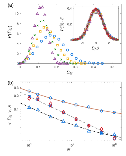
Figure 9: (a) The probability distribution $P(\hat{\Sigma}_{N})$ of the normal stress difference for MS packings generated via protocol 2 with pure shear for $N=32$ (circles), $64$ (squares), $128$ (crosses), and $256$ (triangles). The inset shows the distributions for ${\hat{\Sigma}}_{N}$ (same symbols as in main panel) and $\hat{\Sigma}_{xy}$ (same symbols as in main panel, but in red) for MS packings generated via protocol 1, and $\hat{\Sigma}_{xy}$ for MS packings generated via protocol 2 using pure shear (same symbols as in main panel, but in gray). The solid black line is a Gaussian distribution with a zero mean and unit standard deviation. (b) System-size dependence of 1) the average (circles) and standard deviation (triangles) of $P({\hat{\Sigma}}_{N})$ for MS packings generated via protocol 2 with pure shear, 2) standard deviation of $P({\hat{\Sigma}}_{xy})$ (squares) for MS packings generated via protocol 2 with pure shear, and 3) standard deviations of $P({\hat{\Sigma}}_{N})$ (crosses) and $P({\hat{\Sigma}}_{xy})$ (diamonds) for MS packings generated via protocol 1. The dashed, solid, and dash-dotted lines are fits to Eqs. 3, 19, and 20, respectively.

The average of $P({\hat{\Sigma}}_{N})$ for MS packings generated via protocol 2 with pure shear decreases as $N$ increases, but reaches a nonzero value in the large-system limit:

$$\langle\hat{\Sigma}_{N}\rangle(N)=\hat{\Sigma}_{0}N^{-\Omega}+\hat{\Sigma}_{\infty},$$ (19)

where $\hat{\Sigma}_{0}\approx 0.49$, $\Omega\approx 0.40$, and $\hat{\Sigma}_{\infty}\approx 0.055$. Similarly, the standard deviation of $P({\hat{\Sigma}}_{N})$ also reaches a nonzero value in the large-system limit:

$$S_{2}(N)=S_{2}^{0}N^{-\omega_{2}}+S_{\infty},$$ (20)

where $S_{2}^{0}\approx 0.30$, $\omega_{2}\approx 0.50$, and $S_{\infty}\approx 0.016$. The results for MS packings generated via protocol 2 with pure shear are analogous to those observed for MS packings generated via protocol 2 with simple shear. (See Table 1.)

MS packings generated via protocol 2 for pure shear obey the same stress-dilatancy relationship (Eq. 2) as that for simple shear. Thus, we can apply the statistical model in Sec.  III.3 to predict the stress anisotropy distribution for MS packings generated via pure shear. As shown in Fig.  10 (a) and (b), the distribution for the dilatancy of shear-jammed packings at small $\gamma$ limit obeys a Weibull distribution, which can be predicted from the half-Gaussian distribution for MS packings obtained via protocol 1. (See Eqs.  9 and  10.) The conditional probability, $P_{2}(\dot{\phi}|\gamma)$, for obtaining $\dot{\phi}$ at a given $\gamma$ is shown in Fig.  10 (c) and fit to a Weibull distribution $f_{w}(\dot{\phi};\gamma,k)$. In Fig.  10 (d), we plot the $\gamma$ dependence of the shape $k(\gamma)$ and scale $\lambda(\gamma)$ parameters. Both parameters decay exponentially to steady-state values in the large-$\gamma$ limit. (See Eq. 12.) These results are similar to those for simple shear case described in the main text.

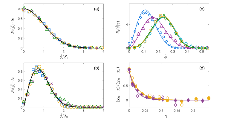
Figure 10: (a) Probability distribution of the dilatancy $P_{1}(\dot{\phi})$ for $\dot{\phi}>0$ scaled by the standard deviation $S_{1}$ for MS packings generated via protocol 1 and pure shear with $N=64$ (squares), $128$ (circles), $256$ (triangles), and $512$ (crosses). The solid line is the half-Gaussian distribution in Eq. 9. (b) Probability distribution of the dilatancy $P(\dot{\phi})$ for MS packings generated via protocol 2 with pure shear in the small strain limit ($\gamma<2\times 10^{-4}$). The symbols are the same as in panel (a). The solid line is the Weibull distribution in Eq. 10 with shape parameter $k_{0}=2$ and scale parameter $\lambda_{0}=\sqrt{2}S_{1}$. (c) The conditional probability $P_{2}(\dot{\phi}|\gamma)$ for obtaining dilatancy ${\dot{\phi}}$ for MS packings with $N=128$ generated via protocol 2 with pure shear for $\gamma<2\times 10^{-4}$ (circles), $0.010<\gamma<0.0105$ (triangles), $0.18<\gamma<0.20$ (diamonds), $0.20<\gamma<0.22$ (squares), and $0.24<\gamma<0.26$ (crosses). The solid lines are Weibull distributions $f_{w}({\dot{\phi}},\lambda(\gamma),k(\gamma))$. （d) The $\gamma$-dependence of the shape parameter $\chi=k$ (open symbols) and scale parameter $\chi=\lambda$ (solid symbols) for fits of $P_{2}({\dot{\phi}}|\gamma)$ to Weibull distributions for $N=128$ (circles) and $512$ (diamonds). $\chi_{0}$ and $\chi_{\infty}$ give the values of $k$ and $\lambda$ at $\gamma=0$ and in the $\gamma\rightarrow\infty$ limit, respectively. The solid lines are fits to an exponential decay, $\sim\exp(-\gamma/\gamma_{c})$, where $\gamma_{c}=0.029$ and $0.021$ for $N=128$ and $512$, respectively.

Appendix B: Protocol dependence of the volume of the basin of attraction for MS packings

In the description of the statistical framework (Sec. III.3) for calculating the distribution of dilatancy for MS packings generated via protocol 2 with simple shear from those generated via protocol 1, we first assumed that the volumes of the basins of attraction were the same (i.e. $V_{1,i}\approx V_{2,i}$) for protocols 1 and 2. In this Appendix, we illustrate that this assumption breaks down for sufficiently large simple shear strains.

We illustrate the basin volume for an $N=6$ MS packing, which is a four-dimensional quantity, by projecting it into two dimensions. We consider a particular $N=6$ MS packing at shear strain $\gamma$ and packing fraction $\phi$ that can be generated readily via protocol 1 and protocol 2 with simple shear. We identify a point $(\mathbf{r}_{1},\mathbf{r}_{2},\ldots,\mathbf{r}_{6})$ within the basin of attraction of the MS packing and constrain the positions of particles $2$ through $6$. The initial position of particle $1$ is allowed to vary in the $x$-$y$ plane. The pixels in each panel of Fig. 11 represent the initial positions of particle $1$ and they are colored blue if the initial configuration at ($x$,$y$) maps to the position of particle $1$ in the particular MS packing that we selected. The area of the blue region gives the projected area of the basin of attraction for that particular MS packing.

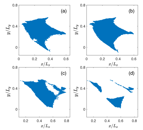
Figure 11: Two-dimensional projection of the four-dimensional basin of attraction for a particular $N=6$ MS packing generated using (a) protocol 1 and (b) protocol 2 (with simple shear) at shear strain $\gamma=2\times 10^{-3}$. The $x$- and $y$-coordinates indicate the initial position of particle $1$, while the initial conditions for particles $2$ through $6$ are fixed to specific locations within the simulation cell. If a pixel is blue, the initial position maps to the target MS packing after the packing-generation procedure. Panels (c) and (d) are comparable to (a) and (b) except the shear strain has been increased to $\gamma=0.02$.

In Fig. 11 (a) and (b), we show the basins of attraction for a particular MS packing at a small shear strain, $\gamma=2\times 10^{-3}$, for protocols 1 and 2, respectively. The areas of the blue regions are nearly the same, which suggests that $V_{1,i}\approx V_{2,i}$. However, at larger shear strains, the basin volumes for the two protocols deviate. For example, in Fig. 11 (c) and (d) at shear strain $\gamma=0.02$, the projected area for protocol 1 is much larger than that for protocol 2, which implies that $V_{1,i}\neq V_{2,i}$.

Appendix C: Simple shear of circulo-triangle packings

In this Appendix, we show that MS packings of non-spherical particles, specifically circulo-triangles, also form geometrical families in the packing fraction $\phi$ and shear strain $\gamma$ plane. We considered bidisperse mixtures of circulo-triangles, half large and half small with area ratio $r_{a}=1.4^{2}$ and interior angles of $33^{\circ}$, $62^{\circ}$, and $85^{\circ}$ for each triangle. We fixed the asphericity parameter $\mathcal{A}=p^{2}/4\pi a=1.1$, where $p$ and $a$ are the perimeter and area of the circulo-triangles, respectively. At this asphericity, the packings can be either isostatic or hypostatic VanderWerf et al. (2018).

As is the case for circular disks, we find that the geometrical families for MS packings of circulo-triangles generated via protocol 1 with simple shear form parabolic segments in the $\phi$-$\gamma$ plane, satisfying $\phi(\gamma)=A(\gamma-\gamma_{0})^{2}+\phi_{0}$. However, we find that the curvature of the parabolas can be both concave up and concave down ($A>0$ and $A<0$) for MS packings of circulo-triangles. In contrast, $A>0$ for MS disk packings. $A<0$ implies strain-induced compaction, which may be caused by the alignment of the circulo-triangles during shear. Preliminary results indicate that the stress anisotropy for shear jammed packings of circulo-triangles is finite (and larger than that for frictionless disks) in the large system limit.

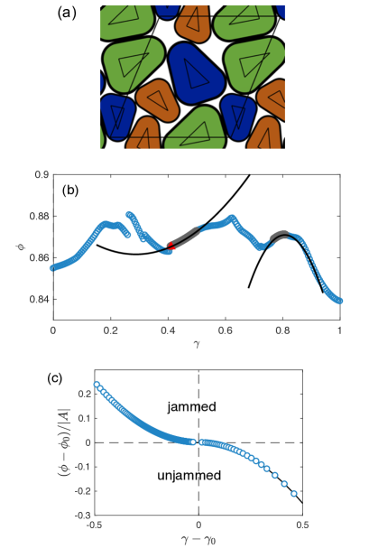
Figure 12: (a) An MS packing of $N=6$ of bidisperse circulo-triangles with asphericity parameter ${\cal A}=1.1$. (b) Packing fraction $\phi$ at jamming onset as a function of simple shear strain $\gamma$ for $N=6$ MS packings of circulo-triangles generated via protocol 1. The packing in panel (a) corresponds to the filled red triangle. The solid lines are fits of two particular parabolic regions (shaded gray) to $\phi(\gamma)=A(\gamma-\gamma_{0})^{2}+\phi_{0}$. (c) $(\phi-\phi_{0})/|A|$ versus $\gamma-\gamma_{0}$, for $N=6$ MS packings of circulo-triangles generated via protocol 2 with simple shear. These packings populate the parabolic regions with $d\phi/d\gamma<0$ on segments with both $A>0$ and $A<0$. The jammed and unjammed regions of the $(\phi-\phi_{0})/|A|$ and $\gamma-\gamma_{0}$ plane are indicated.

References

- McQuarrie (2000) D. A. M. McQuarrie, Statistical Mechanics, University Science Books, 2000.
- Jaeger et al. (1996) H. M. Jaeger, S. R. Nagel and R. P. Behringer, Reviews of Modern Physics, 1996, 68, 1259.
- Baule et al. (2018) A. Baule, F. Morone, H. J. Herrmann and H. A. Makse, Reviews of Modern Physics, 2018, 90, 015006.
- Gao et al. (2006) G.-J. Gao, J. Bławzdziewicz and C. S. O’Hern, Physical Review E, 2006, 74, 061304.
- Shen et al. (2014) T. Shen, S. Papanikolaou, C. S. O’Hern and M. D. Shattuck, Physical Review Letters, 2014, 113, 128302.
- Gao et al. (2009) G.-J. Gao, J. Blawzdziewicz, C. S. O’Hern and M. Shattuck, Physical Review E, 2009, 80, 061304.
- Majmudar and Behringer (2005) T. S. Majmudar and R. P. Behringer, Nature, 2005, 435, 1079.
- Bi et al. (2011) D. Bi, J. Zhang, B. Chakraborty and R. P. Behringer, Nature, 2011, 480, 355.
- Bertrand et al. (2016) T. Bertrand, R. P. Behringer, B. Chakraborty, C. S. O’Hern and M. D. Shattuck, Physical Review E, 2016, 93, 012901.
- Clusel et al. (2009) M. Clusel, E. I. Corwin, A. O. Siemens and J. Brujić, Nature, 2009, 460, 611.
- O’Hern et al. (2003) C. S. O’Hern, L. E. Silbert, A. J. Liu and S. R. Nagel, Physical Review E, 2003, 68, 011306.
- Kumar and Luding (2016) N. Kumar and S. Luding, Granular Matter, 2016, 18, 58.
- Baity-Jesi et al. (2017) M. Baity-Jesi, C. P. Goodrich, A. J. Liu, S. R. Nagel and J. P. Sethna, Journal of Statistical Physics, 2017, 167, 735–748.
- Xu and O’Hern (2006) N. Xu and C. S. O’Hern, Physical Review E, 2006, 73, 061303.
- Clark et al. (2015) A. H. Clark, M. D. Shattuck, N. T. Ouellette and C. S. O’Hern, Physical Review E, 2015, 92, 042202.
- VanderWerf et al. (2018) K. VanderWerf, W. Jin, M. D. Shattuck and C. S. O’Hern, Physical Review E, 2018, 97, 012909.
- Lees and Edwards (1972) A. Lees and S. Edwards, Journal of Physics C: Solid State Physics, 1972, 5, 1921.
- Tanguy et al. (2002) A. Tanguy, J. Wittmer, F. Leonforte and J.-L. Barrat, Physical Review B, 2002, 66, 174205.
- Tkachenko and Witten (1999) A. V. Tkachenko and T. A. Witten, Physical Review E, 1999, 60, 687.
- Gao et al. (2009) G.-J. Gao, J. Blawzdziewicz and C. S. O’Hern, Physical Review E, 2009, 80, 061303.
- Peyneau and Roux (2008) P.-E. Peyneau and J.-N. Roux, Physical Review E, 2008, 78, 011307.
- Kabla and Senden (2009) A. J. Kabla and T. J. Senden, Physical Review Letters, 2009, 102, 228301.
- Kruyt and Rothenburg (2006) N. P. Kruyt and L. Rothenburg, Journal of Statistical Mechanics: Theory and Experiment, 2006, 2006, P07021.
- Zheng et al. (2018) W. Zheng, S. Zhang and N. Xu, arXiv preprint arXiv:1804.08054, 2018.
- Xu et al. (2011) N. Xu, D. Frenkel and A. J. Liu, Physical Review Letters, 2011, 106, 245502.
- Ashwin et al. (2012) S. Ashwin, J. Blawzdziewicz, C. S. O’Hern and M. D. Shattuck, Physical Review E, 2012, 85, 061307.
- Otsuki and Hayakawa (2017) M. Otsuki and H. Hayakawa, Physical Review E, 2017, 95, 062902.
- Cundall and Strack (1979) P. A. Cundall and O. D. Strack, Geotechnique, 1979, 29, 47–65.