Statistical inference for heavy tailed series with extremal independence

Abstract

We consider stationary time series $\{X_{j},j\in\mathbb{Z}\}$ whose finite dimensional distributions are regularly varying with extremal independence. We assume that for each $h\geq 1$, conditionally on $X_{0}$ to exceed a threshold tending to infinity, the conditional distribution of $X_{h}$ suitably normalized converges weakly to a non degenerate distribution. We consider in this paper the estimation of the normalization and of the limiting distribution.

1 Introduction

Let $\{X_{j},j\in\mathbb{Z}\}$ be a strictly stationary univariate time series. We say that the time series $\{X_{j}\}$ is regularly varying if all its finite dimensional distributions are regularly varying, i.e. for each $h\geq 0$, there exists a nonzero boundedly finite measure ${\boldsymbol{\nu}}_{\boldsymbol{h}}$ on $\mathbb{R}^{h+1}\setminus\{\boldsymbol{0}\}$ infinity, such that

$$\frac{\mathbb{P}\left(x^{-1}(X_{0},\dots,X_{h})\in\cdot\right)}{\mathbb{P}(|X_{0}|>x)}\stackrel{{\scriptstyle\mbox{\tiny\rm v}}}{{\longrightarrow}}{\boldsymbol{\nu}}_{\boldsymbol{h}}\;,$$ (1.1)

on $\mathbb{R}^{h+1}\setminus\{\boldsymbol{0}\}$, as $x\to\infty$, where $\stackrel{{\scriptstyle\mbox{\tiny\rm v}}}{{\longrightarrow}}$ means vague convergence. Following [Kal17], we say that a measure $\nu$ defined on a complete separable metric space $E$ (endowed with its Borel $\sigma$-field) is boundedly finite if $\nu(B)$ for all Borel bounded sets and a sequence of boundedly finite measures $\{\nu_{n}\}$ is said to converge vaguely to a measure $\nu$ if $\nu_{n}(f)\to\nu(f)$ for all continuous functions with bounded support. See also [HL06] who use the terminology of $\mathcal{M}_{0}$-convergence. Here the metric space considered is $\mathbb{R}^{h+1}\setminus\{{\boldsymbol{0}}\}$ endowed with the metric

$$d_{h}(\boldsymbol{x},\boldsymbol{y})=\left|\boldsymbol{x}-\boldsymbol{y}\right|\vee|\left|\boldsymbol{x}\right|^{-1}-\left|\boldsymbol{y}\right|^{-1}|\;,$$

where $\left|\cdot\right|$ is an arbitrary norm on $\mathbb{R}^{h+1}$. This metric induces the usual topology and makes $\mathbb{R}^{h+1}\setminus\{{\boldsymbol{0}}\}$ a complete separable space and bounded sets are sets separated from zero. Moreover, $\mathbb{R}^{h+1}\setminus\{{\boldsymbol{0}}\}$ is still locally compact so this definition essentially yields the same notion as the classical vague convergence without the need for compactification at infinity.

This assumption implies that there exists $\alpha>0$ such that the measure ${\boldsymbol{\nu}}_{\boldsymbol{h}}$ is homogeneous of degree $-\alpha$ and the marginal distribution of $X_{0}$ is regularly varying and satisfies the balanced tail condition: there exists $p\in[0,1]$ such that

$$p=\lim_{x\to\infty}\frac{\mathbb{P}(X_{0}>x)}{\mathbb{P}(|X_{0}|>x)}=1-\lim_{x\to\infty}\frac{\mathbb{P}(X_{0}<-x)}{\mathbb{P}(|X_{0}|>x)}\;.$$

Without loss of generality, we assume that $p>0$.

If $h\geq 1$, there exist two fundamentally different cases: either the exponent measure is concentrated on the axes or it is not. The former case is referred to as extremal independence and the latter as extremal dependence. In other words, extremal independence means that no two components can be extremely large at the same time, and extremal dependence means that some pairs components can be simultaneously extremely large.

In a time series context, we may want to assess the influence of an extreme event at time zero on future observations. If the finite dimensional distributions of the time series model under consideration are extremally independent or more generally if the vector $(X_{0},X_{m},\dots,X_{h})$ is extremally independent for some $h\geq m\geq 1$, then, for any Borel set $A$ which is bounded away from zero in $\mathbb{R}^{h-m+1}$ and $y_{0}>0$,

$$\lim_{x\to\infty}\frac{\mathbb{P}(X_{0}>xy_{0},(X_{m}\dots,X_{h})\in xA)}{\mathbb{P}(|X_{0}|>x)}=0\;.$$ (1.2)

Thus in case of extremal independence the exponent measure ${\boldsymbol{\nu}}_{\boldsymbol{h}}$ provides no information on (most) extreme events occurring after an extreme event at time 0.

In order to obtain a non degenerate limit in (1.2) and a finer analysis of the sequence of extreme values, it is necessary to change the normalization in (1.1), and possibly the space on which we will assume that vague convergence holds. One idea is to find a sequence of normalizations $b_{j}(x)$, $j\geq 1$ such that for each $h\geq 1$, the conditional distribution of $(X_{0}/x,X_{1}/b_{1}(x),\dots,X_{h}(x)/b_{h}(x))$ given $|X_{0}|>x$ has a non degenerate limit. Pursuing in the direction opened by [HR07] and [DR11], [LRR14] and [KS15] we will consider vague convergence on the set $(\mathbb{R}\setminus\{0\})\times\mathbb{R}^{h}$ endowed with the metric $d_{h}^{0}$ on defined by

$$d_{h}^{0}(\boldsymbol{x},\boldsymbol{y})=\left|\boldsymbol{x}-\boldsymbol{y}\right|\vee|x_{0}^{-1}-y_{0}^{-1}|\;.$$

The bounded sets for this metric are those sets $A$ such that $\boldsymbol{x}=(x_{0},\dots,x_{h})\in A$ implies $|x_{0}|>\epsilon$ for some $\epsilon>0$. Note that under the present definition of vague convergence, we avoid the pitfalls described in [DJe17].

Assumption 1.1.

There exist scaling functions $b_{j}$, $j\geq 1$ and nonzero measures $\boldsymbol{\mu}_{0,h}$, $h\geq 1$, boundedly finite on $(\mathbb{R}\setminus\{0\})\times\mathbb{R}^{h}$, $h\geq 1$, such that

$$\frac{1}{\mathbb{P}(|X_{0}|>x)}\mathbb{P}\left(\left(\frac{X_{0}}{x},\frac{X_{1}}{b_{1}(x)},\cdots,\frac{X_{h}}{b_{h}(x)}\right)\in\cdot\right)\stackrel{{\scriptstyle\mbox{\tiny\rm v}}}{{\longrightarrow}}\boldsymbol{\mu}_{0,h}\;,$$ (1.3)

on $(\mathbb{R}\setminus\{0\})\times\mathbb{R}^{h}$ and for every $y_{0}>0$, the measures $\boldsymbol{\mu}_{0,h}([y_{0},\infty)\times\cdot)$ and $\boldsymbol{\mu}_{0,h}((-\infty,-y_{0})\times\cdot)$ on $\mathbb{R}^{h}$ are not concentrated on a hyperplane.

This assumption does not exclude regularly varying time series with extremal dependence for which $b_{j}(x)=x$ for all $j\geq 0$. But our interest will be in extremally independent time series for which $b_{j}(x)=o(x)$ for all $j\geq 0$. This assumption is fulfilled by many time series, like stochastic volatility models with heavy tailed noise or heavy tailed volatility, exponential moving averages and certain Markov chains with regularly varying initial distribution and appropriate conditions on the transition kernel. See [KS15], [MR13] and [JD16].

An important consequence of Assumption 1.1 is that the functions $b_{j}$, $j\geq 1$ are regularly varying (see [HR07, Proposition 1] and [KS15].) To put emphasis on the regular variation of the functions $b_{j}$, we recall the following definition of [KS15].

Definition 1.2 (Conditional scaling exponent).

Under Assumption 1.1, for $h\geq 1$, we call the index $\kappa_{h}$ of regular variation of the functions $b_{h}$ the (lag $h$) conditional scaling exponent.

The exponents $\kappa_{h}$, $h\geq 1$ reflect the influence of an extreme event at time zero on future lags. Even though we expect this influence to decrease with the lag in the case of extremal independence, these exponents are not necessarily monotone decreasing. The measures $\boldsymbol{\mu}_{0,h}$ also have some important homogeneity properties: For all Borel sets $A_{0}\subset\mathbb{R}\setminus\{0\}$, $A_{1},\dots,A_{h}\subset\mathbb{R}$,

$$\boldsymbol{\mu}_{0,h}\left(tA_{0}\times\prod_{i=1}^{h}t^{\kappa_{i}}A_{i}\right)=t^{-\alpha}\boldsymbol{\mu}_{0,h}\left(\prod_{i=0}^{h}A_{i}\right)\;.$$ (1.4)

Equivalently, for all bounded measurable functions $f$,

$$\int_{(\mathbb{R}\setminus\{0\})\times\mathbb{R}^{h}}f(t^{-1}x_{0},t^{-\kappa_{1}}x_{1},\dots,t^{-\kappa_{h}}x_{h})\boldsymbol{\mu}_{0,h}(\mathrm{d}\boldsymbol{x})=t^{-\alpha}\int_{(\mathbb{R}\setminus\{0\})\times\mathbb{R}^{h}}f(\boldsymbol{x})\boldsymbol{\mu}_{0,h}(\mathrm{d}x)\;.$$ (1.5)

Cf. [HR07, Proposition 1] and [KS15, Lemma 2.1]. Define the probability measure $\boldsymbol{\sigma}_{h}$ on $\{-1,1\}\times\mathbb{R}^{h}$ by

$$\boldsymbol{\sigma}_{h}(\{\epsilon\}\times A)=\int_{\epsilon u_{0}>1}\int_{A}\boldsymbol{\mu}_{0,h}(\mathrm{d}u_{0},u_{0}^{\kappa_{1}}\mathrm{d}u_{1},\dots,u_{0}^{\kappa_{h}}\mathrm{d}u_{h})\;,$$

for $\epsilon\in\{-1,1\}$ and $A$ a Borel subset of $\mathbb{R}^{h}$. Let $\boldsymbol{W}=(W_{0},W_{1},\dots,W_{h})$ be an $\mathbb{R}^{h+1}$ valued random vector with distribution $\boldsymbol{\sigma}_{h}$. Then, for every Borel subsets $A\subset\left(\mathbb{R}\setminus\{0\}\right)\times\mathbb{R}^{h}$, we have

$$\boldsymbol{\mu}_{0,h}(A)=\int_{0}^{\infty}\mathbb{P}((sW_{0},s^{\kappa_{1}}W_{1},\dots,s^{\kappa_{h}}W_{h})\in A)\,\alpha s^{-\alpha-1}\mathrm{d}s\;.$$ (1.6)

See [KS15, Section 2.4]. Let $Y_{0}$ be a Pareto random variable with tail index $\alpha$, independent of $\boldsymbol{W}_{h}$. Then, as $x\to\infty$,

$$\mathcal{L}\left(\left(\frac{X_{0}}{x},\frac{X_{1}}{b_{1}(x)},\dots,\frac{X_{h}}{b_{h}(x)}\right)\mid|X_{0}|>x\right)\stackrel{{\scriptstyle\mbox{\tiny\rm d}}}{{\longrightarrow}}Y_{0}\boldsymbol{W}_{h}\;.$$ (1.7)

In particular, we define for $h>0$ the distribution function $\Psi_{h}$ on $\mathbb{R}$:

$$\Psi_{h}(y) =\mathbb{P}(Y_{0}W_{h}\leq y)=\lim_{x\to\infty}\mathbb{P}(X_{h}\leq b_{h}(x)y\mid|X_{0}|>x)\;,$$ (1.8)

for all $y\in\mathbb{R}\setminus\{0\}$ since the distribution of $Y_{0}W_{h}$ is continuous at all points except possibly 0.

The goal of this paper is to complement the investigation of this assumption started in [KS15] by providing valid statistical procedures to estimate the conditional scaling functions $b_{h}$, the conditional limiting distributions $\Psi_{h}$ and scaling exponents $\kappa_{h}$.

2 Statistical inference

Let $F_{0}$ be a distribution of $|X_{0}|$. All our results we be proved under the following $\beta$-mixing assumptions.

Assumption 2.1.

1. The sequence $\{X_{j},j\in\mathbb{Z}\}$ is $\beta$-mixing with rate $\{\beta_{n},n\geq 1\}$.

2. There exist a non decreasing sequence $u_{n}$, non decreasing sequences of integers $r_{n}$ and $l_{n}$ such that

   $$\lim_{n\to\infty}l_{n} =\lim_{n\to\infty}r_{n}=\lim_{n\to\infty}u_{n}=\lim_{n\to\infty}\frac{r_{n}}{l_{n}}=\infty\;,$$ (2.1)

   $$\lim_{n\to\infty}\frac{n}{r_{n}}\beta_{l_{n}} =0\;,$$ (2.2)

   $$\lim_{n\to\infty}u_{n} =n\bar{F}_{0}(u_{n})=\infty\;,\ \ \lim_{n\to\infty}r_{n}\bar{F}_{0}(u_{n})=0\;.$$ (2.3)

2.1 Non parametric estimation of the limiting conditional distribution

In order to define an estimator of $\Psi_{h}$, we must first consider the infeasible statistic

$$\widetilde{I}_{h,n}(s,y) =\frac{1}{n\overline{F_{0}}(u_{n})}\sum_{j=1}^{n-h}\mathbbm{1}{\left\{|X_{j}|>u_{n}s,X_{j+h}\leq b_{h}(u_{n})y\right\}}\;.$$ (2.4)

Then, Assumption 1.1 and the homogeneity property (1.5) imply that for all $s>0$ and $y\in\mathbb{R}$,

$$\lim_{n\to\infty}\mathbb{E}[\widetilde{I}_{h,n}(s,y)] =\lim_{n\to\infty}\frac{n-h}{n}\frac{\mathbb{P}(|X_{0}|>u_{n}s,X_{h}\leq b(u_{n})y)}{\overline{F}_{0}(u_{n})}$$

$$=\boldsymbol{\mu}_{0,h}((s,\infty)\times\mathbb{R}^{h-1}\times(-\infty,y])=s^{-\alpha}\Psi_{h}(s^{-\kappa_{h}}y)\;.$$

We consider weak convergence of the processes $\widetilde{\mathbb{I}}_{h,n}$ and $\mathbb{I}_{h,n}$ defined on $(0,\infty)\times\mathbb{R}$ by

$$\widetilde{\mathbb{I}}_{h,n}(s,y) =\sqrt{n\overline{F_{0}}(u_{n})}\{\widetilde{I}_{h,n}(s,y)-\mathbb{E}[\widetilde{I}_{h,n}(s,y)]\}\;,$$

$$\mathbb{I}_{h,n}(s,y) =\sqrt{n\overline{F_{0}}(u_{n})}\{\widetilde{I}_{h,n}(s,y)-s^{-\alpha}\Psi_{h}(s^{-\kappa_{h}}y)\}\;.$$

Assumption 2.2.

For all $s,t>0$,

$$\lim_{\ell\to\infty}\limsup_{n\to\infty}\frac{1}{\overline{F}_{0}(u_{n})}\sum_{\ell<|j|\leq r_{n}}\mathbb{P}(|X_{0}|>u_{n}s,|X_{j}|>u_{n}t)=0\;.$$ (2.5)

Assumption 2.3.

There exists $s_{0}\in(0,1)$ such that

$$\lim_{n\to\infty}\sqrt{n\overline{F}_{0}(u_{n})}\sup_{s\geq s_{0},y\in\mathbb{R}}\left|\frac{\mathbb{P}(|X_{0}|>u_{n}s,X_{h}\leq b(u_{n})y)}{\overline{F}_{0}(u_{n})}-s^{-\alpha}\Psi_{h}(s^{-\kappa_{h}}y)\right|=0\;.$$ (2.6)

Remark 2.4.

An assumptions similar to (2.5) is unavoidable. Its purpose is to prove the convergence of the intrablock variance in the blocking method and tightness. The present one is taken from [KSW15]. Similar ones have been considered in [Roo09], [DR10] and [DSW15]. Some of these conditions have been checked directly for extremally dependent time series like GARCH(1,1) or ARMA models (see e.g. [Dre02]), or for Markov chains that satisfy a drift condition (cf. [KSW15]). This assumption will be checked in Section 3 for some specific models. Assumption 2.3 is unavoidable if one wants to remove bias. This will not be discussed in the paper. The condition holds for some sequences $u_{n}$.

Let $\mathbb{I}_{h}$ be a the Gaussian process on $(0,\infty)\times\mathbb{R}$ with covariance $\mathrm{cov}(\mathbb{I}_{h}(s,y),\mathbb{I}_{h}(t,z))=(s\vee t)^{-\alpha}\Psi_{h}((s\vee t)^{-\kappa_{h}}(y\wedge z))$, $s,t>0$, $y,z\in\mathbb{R}$. We note that

$$\mathbb{W}(u)=\mathbb{I}_{h}(1,\Psi_{h}^{-1}(u))\;,\ \ u\in(0,1)\;,$$

is a standard Brownian motion on $(0,1)$. The following theorem establishes weak convergence of the tail empirical process and forms the basis for statistical inference on $\Psi_{h}$. Its proof is given in Section 6.2.

Theorem 2.5.

Let $\{X_{j},j\in\mathbb{Z}\}$ be a strictly stationary regularly varying sequence such that Assumption 1.1 with extremal independence at all lags. Assume moreover that Assumptions 2.1 and 2.2 hold and that the function $\Psi_{h}$ is continuous on $\mathbb{R}$. Then the process $\widetilde{\mathbb{I}}_{h,n}$ converges weakly in $\ell^{\infty}([s_{0},\infty)\times\mathbb{R})$ to $\mathbb{I}_{h}$. If moreover Assumption 2.3 holds, then $\mathbb{I}_{h,n}$ converges weakly in $\ell^{\infty}([s_{0},\infty)\times\mathbb{R})$ to $\mathbb{I}_{h}$.

We now need proxies to replace $u_{n}$ and $b(u_{n})$ which are unknown in order to obtain a feasible statistical procedure. As usual, $u_{n}$ will be replaced by an order statistic. To estimate the scaling functions $b_{h}$ we will exploit their representations in terms of conditional mean. Therefore, we need additional conditions.

Assumption 2.6.

There exists $\delta>0$ and $s_{0}>0$ such that

$$\lim_{n\to\infty}r_{n}\{n\overline{F}_{0}(u_{n})\}^{-\delta/2}=0\;,$$ (2.7)

$$\sup_{n\geq 1}\frac{1}{\overline{F}_{0}(u_{n})}\mathbb{E}\left[\left|\frac{X_{h}}{b_{h}(u_{n})}\right|^{2+\delta}\mathbbm{1}{\left\{\{X_{0}>s_{0}u_{n}\}\right\}}\right]<\infty\;,$$ (2.8)

$$\lim_{\ell\to\infty}\limsup_{n\to\infty}\frac{1}{\overline{F}_{0}(u_{n})}\sum_{\ell<|j|\leq r_{n}}\mathbb{E}\left[\frac{|X_{h}|}{b_{h}(u_{n})}\frac{|X_{j+h}|}{b_{h}(u_{n})}\mathbbm{1}{\left\{\{X_{0}>s_{0}u_{n}\}\right\}}\mathbbm{1}{\left\{\{X_{j}>s_{0}u_{n}\}\right\}}\right]=0\;,$$ (2.9)

$$\lim_{n\to\infty}\sup_{s\geq s_{0}}\sqrt{n\overline{F}_{0}(u_{n})}\left|\frac{\mathbb{E}\left[\frac{|X_{h}|}{b_{h}(u_{n})}\mathbbm{1}{\left\{|X_{0}|>u_{n}s\right\}}\right]}{\overline{F}_{0}(u_{n})}-\mathbb{E}[|W_{h}|]s^{\kappa_{h}-\alpha}\right|=0\;.$$ (2.10)

Condition (2.8) requires $\alpha>2$ and implies that the sequence $(b_{h}^{-1}(u_{n})X_{h})^{2}$ is uniformly integrable conditionally on $|X_{0}|>u_{n}$ and therefore,

$$\lim_{x\to\infty}\mathbb{E}\left[b_{h}^{-i}(x)|X_{h}|^{i}\mid X_{0}>x\right]=\int_{-\infty}^{\infty}|y|^{i}\,\Psi_{h}(\mathrm{d}y)=\mathbb{E}[Y_{0}^{i}]\mathbb{E}[|W_{h}|^{i}]<\infty\;,\ \ i=1,2\;.$$ (2.11)

Since the function $b_{h}$ and the limiting distribution $\Psi_{h}$ are defined up to a scaling constant, we can and will assume without loss of generality that

$$\mathbb{E}[|W_{h}|]=\int_{-\infty}^{\infty}|y|\,\Psi_{h}(\mathrm{d}y)=\int_{1}^{\infty}\int_{-\infty}^{\infty}|x_{h}|\boldsymbol{\mu}_{0,h}(\boldsymbol{x})\;.$$

Condition (2.9) is again unavoidable and must be checked for specific models. Condition (2.10) is a bias condition which will not be further discussed.

Set $k=n\overline{F}_{0}(u_{n})$ and let $|X|_{(n:1)}\leq|X|_{(n:2)}\leq\cdots\leq|X|_{(n:n)}$ be the order statistics of $|X_{1}|,\ldots,|X_{n}|$. Define an estimator of $b_{h}(u_{n})$ by

$$\widehat{b}_{h,n}=\frac{1}{k}\sum_{j=1}^{n-h}|X_{j+h}|\mathbbm{1}{\left\{\{|X_{j}|>|X|_{(n:n-k)}\}\right\}}\;.$$ (2.12)

Corollary 2.7.

Let the assumptions of Theorem 2.5 and Assumption 2.6 hold with extremal independence at all lags. Then

$$\left(\mathbb{I}_{h,n},\sqrt{k}\left(\frac{|X|_{(n:n-k)}}{u_{n}}-1\right),\sqrt{k}\left(\frac{\widehat{b}_{h,n}}{b_{h}(u_{n})}-1\right)\right)\\ \stackrel{{\scriptstyle\mbox{\tiny\rm w}}}{{\longrightarrow}}\left(\mathbb{I}_{h},\alpha^{-1}\mathbb{W}(1),\int_{0}^{1}|\Psi_{h}^{-1}(u)|\mathrm{d}\mathbb{B}(u)+\alpha^{-1}\kappa_{h}\mathbb{W}(1)\right)\;,$$

where $\mathbb{W}(u)=\mathbb{I}_{h}(1,\Psi_{h}^{-1}(u))$ is a standard Brownian motion and $\mathbb{B}(u)=\mathbb{W}(u)-u\mathbb{W}(1)$ is a standard Brownian bridge on $[0,1]$.

Remark 2.8.

The moment conditions in Assumption 2.6 may seem to be too restrictive. In fact, we can consider a family of estimators $\widehat{b}_{h,n}(\zeta)$, where $|X_{j+h}|$ in (2.12) is replaced with $|X_{j+h}|^{\zeta}$ with some $\zeta>0$. However, we do not pursue it in this paper.

Define now the following estimator of $\Psi_{h}$:

$$\widehat{\Psi}_{h,n}(y)=\frac{1}{k}\sum_{j=1}^{n-h}\mathbbm{1}{\left\{\{X_{j}>X_{(n:n-k)}\}\right\}}\mathbbm{1}{\left\{\{X_{j+h}\leq\widehat{b}_{h,n}y\}\right\}}=\widetilde{I}_{h,n}\left(\frac{X_{(n:n-k)}}{u_{n}},\frac{\widehat{b}_{h,n}}{b_{h}(u_{n})}y\right)\;.$$ (2.13)

The theory for this estimator is easily obtained by applying Corollary 2.7 and the $\delta$-method.

Corollary 2.9.

Under the assumptions of Corollary 2.7 and if the function $\Psi_{h}$ is differentiable, $\sqrt{k}\left\{\widehat{\Psi}_{h,n}-\Psi_{h}\right\}\stackrel{{\scriptstyle\mbox{\tiny\rm w}}}{{\longrightarrow}}\Lambda_{h}$ in $\ell^{\infty}([s_{0},\infty))$, where the process $\Lambda_{h}$ is defined by

$$\Lambda_{h}(y) =\mathbb{B}(\Psi_{h}(y))+y\Psi_{h}^{\prime}(y)\int_{0}^{1}|\Psi_{h}^{-1}(u)|\mathrm{d}\mathbb{B}(u)\;,$$ (2.14)

where $\mathbb{B}$ is the standard Brownian bridge.

Remark 2.10.

The additional term in the limiting distribution is due to the method of estimation of the conditional scaling function. Note that the limiting distribution depends only on $\Psi_{h}$ and therefore can be used for a Kolmogorov-Smirnov type goodness of fit test of the conditional distribution.

2.2 Estimation of the conditional scaling exponent

We now consider the estimation of the scaling exponent $\kappa_{h}$. We will use the following result.

Lemma 2.11.

Let Assumption 1.1 hold and assume moreover that

$$\lim_{\epsilon\to 0}\limsup_{x\to\infty}\frac{\mathbb{P}(|X_{0}X_{h}|>xb_{h}(x),|X_{0}|\leq\epsilon x)}{\mathbb{P}(|X_{0}|>x)}=0\;.$$ (2.15)

Then $\mathbb{E}[|W_{h}|^{\frac{\alpha}{1+\kappa_{h}}}]<\infty$ and

$$\lim_{x\to\infty}\frac{\mathbb{P}(|X_{0}X_{h}|>xb_{h}(x)y)}{\mathbb{P}(|X_{0}|>x)}=\mathbb{E}[|W_{h}|^{\frac{\alpha}{1+\kappa_{h}}}]y^{-\frac{\alpha}{1+\kappa_{h}}}\;.$$ (2.16)

This is [KS15, Proposition 2], where the finiteness of $\mathbb{E}[|W_{h}|^{\frac{\alpha}{1+\kappa_{h}}}]$ is assumed, but it is easily seen that this is actually a consequence of (2.15). At this moment this is all we need to state our results but we will need to prove in Section 6.1 a generalized version of Lemma 2.11; see Lemma 6.4. It must be noted that Condition (2.15) does not hold for an i.i.d. sequence. See also Section 3.1.

If (2.15) holds, then the product $X_{0}X_{h}$ has tail index $\alpha/(1+\kappa_{h})$. Hence, we can suggest the following estimation procedure of the scaling exponent $\kappa_{h}$.

• Let $\gamma=1/\alpha$, where $\alpha$ is the tail index of the sequence $\{|X_{j}|\}$. Estimate $\gamma$ using the Hill estimator $\widehat{\gamma}$ based on an intermediate sequence $k$, i.e.

  $$\hat{\gamma}=\frac{1}{k}\sum_{j=1}^{n}\log(|X|_{(n:n-j+1)}/|X|_{(n:n-k)})\;.$$

• Let $\gamma_{h}=(1+\kappa_{h})\gamma=(1+\kappa_{h})/\alpha$ be estimated by $\widehat{\gamma}_{h}$, the Hill estimator of the tail index of $|X_{0}X_{h}|$, based on the sequence $V_{j}=|X_{j}X_{j+h}|$, $j=1,\dots,n$ (assuming without loss of generality that we have $n+h$ observations) and on the same intermediate sequence:

  $$\hat{\gamma}_{h}=\frac{1}{k}\sum_{j=1}^{n}\log(V_{(n:n-j+1)}/V_{(n:n-k)})\;.$$

• Estimate $\kappa_{h}=\gamma_{h}/\gamma-1$ by

  $$\widehat{\kappa}_{h}={\widehat{\gamma}_{h}}/{\widehat{\gamma}}-1\;.$$ (2.17)

Asymptotic normality of the Hill estimator for beta-mixing sequences is well known. See e.g. [Dre00, Dre02]. The asymptotic normality of $\widehat{\kappa}_{h}$ will follow from the delta method. To state the result, we need additional anti-clustering and second-order conditions.

Assumption 2.12.

For all $s,t>0$,

$$\lim_{\ell\to\infty}\limsup_{n\to\infty}\frac{1}{\overline{F}_{0}(u_{n})}\sum_{\ell<|j|\leq r_{n}}\mathbb{P}(|X_{0}X_{h}|>u_{n}b_{h}(u_{n})s,|X_{j}X_{j+h}|>u_{n}b_{h}(u_{n})t)=0\;.$$ (2.18)

Furthermore,

$$\lim_{\ell\to\infty}\limsup_{n\to\infty} \frac{1}{\overline{F}_{0}(u_{n})}\sum_{j=\ell}^{r_{n}}\mathbb{E}[\log_{+}(|X_{0}|/u_{n})\log_{+}(|X_{j}|/u_{n})]=0\;,$$ (2.19)

$$\lim_{\ell\to\infty}\limsup_{n\to\infty} \frac{1}{\overline{F}_{0}(u_{n})}\sum_{j=\ell}^{r_{n}}\mathbb{E}[\log_{+}(|X_{0}X_{h}|/(u_{n}b(u_{n})))\log_{+}(|X_{j}X_{j+h}|/(u_{n}b(u_{n})))]=0\;.$$ (2.20)

Theorem 2.13.

Let $\{X_{j},j\in\mathbb{Z}\}$ be a strictly stationary regularly varying sequence such that Assumption 1.1 holds with independence at all lags. Assume moreover that Assumptions 2.1, 2.2, 2.12 and 2.3 and the bound (2.15) hold and that $k=n\overline{F}_{0}(u_{n})$ is chosen in such a way that

$$\lim_{n\to\infty}\sqrt{k}\sup_{s\geq s_{0}}\left|\frac{\mathbb{P}(|X_{0}X_{h}|>u_{n}b_{h}(u_{n})s)}{\overline{F}_{0}(u_{n})}-s^{-\alpha/(1+\kappa_{h})}\right|=0$$ (2.21)

for some $s_{0}\in(0,1)$. Then

$$\sqrt{k}(\widehat{\kappa}_{h}-\kappa_{h})\stackrel{{\scriptstyle\mbox{\tiny\rm d}}}{{\longrightarrow}}\mathbf{N}\left(0,(1+\kappa_{h})\mathbb{E}[||W_{h}|^{\frac{\alpha}{1+\kappa_{h}}}-1|]\right)\;.$$

3 Examples

3.1 Stochastic volatility process

Consider the sequence $X_{j}=\varepsilon_{j}\exp(Y_{j})$, $j\in\mathbb{Z}$, where $\{Y_{j},j\in\mathbb{Z}\}$ is a Gaussian process independent of the i.i.d. sequence $\{\varepsilon_{j},j\in\mathbb{Z}\}$, regularly varying with index $\alpha$. For simplicity we assume that the random variables $\varepsilon_{j}$ are nonnegative. We list the properties of $X_{j}$ (see [DM01], [KS11], [KS15]).

1. The sequence $\{X_{j},j\in\mathbb{Z}\}$ is regularly varying with extremal independence. It satisfies Assumption 1.1 with $b_{h}\equiv 1$ for all $h\geq 1$.

2. By Breiman’s lemma, $\mathbb{P}(X_{0}>x)\sim\mathbb{E}[\exp(\alpha Y_{0})]\mathbb{P}(\varepsilon_{0}>x)$ as $x\to\infty$.

3. By [Bra05, Theorem 5.2a),c)], if the spectral density of the Gaussian sequence $\{Y_{j},j\in\mathbb{Z}\}$ is bounded away from zero and if $\mathrm{cov}(Y_{0},Y_{n})=O(n^{-\delta})$ with $\delta>2$ then $\beta(n)=O(n^{2-\delta})$;

4. Conditioning on the sequence ${\mathcal{Y}}=\{Y_{j},j\in\mathbb{Z}\}$, the equivalence between the tails of $\varepsilon_{0}$ and $X_{0}$ and Potter’s bounds yield for $\delta>0$,

   $$\frac{1}{\overline{F_{0}}(u_{n})} \sum_{\ell<|j|\leq r_{n}}\mathbb{P}(X_{0}>u_{n}s,X_{j}>u_{n}s)$$

   $$=\frac{\overline{F}_{\varepsilon}^{2}(u_{n})}{\overline{F_{0}}(u_{n})}\sum_{\ell<|j|\leq r_{n}}\mathbb{E}\left[\frac{\mathbb{P}(\varepsilon_{0}>u_{n}s\exp(-Y_{0})\mid\mathcal{Y})}{\mathbb{P}(\varepsilon_{0}>u_{n})}\frac{\mathbb{P}(\varepsilon_{0}>u_{n}s\exp(-Y_{j})\mid\mathcal{Y})}{\mathbb{P}(\varepsilon_{0}>u_{n})}\right]$$

   $$=O(\overline{F}_{\varepsilon}(u_{n}))\sum_{\ell<|j|\leq r_{n}}\mathbb{E}\left[\exp((\alpha+\delta)(Y_{0}+Y_{j}))\vee 1\right]=O(r_{n}\overline{F_{0}}(u_{n}))=o(1)\;,$$

   as $n\to\infty$ if (2.3) holds.

5. Fix $\delta>0$. We again condition on the sequence $\mathcal{Y}$ and apply Potter’s bounds:

   $$\frac{1}{\overline{F_{0}}(u_{n})} \sum_{\ell<|j|\leq r_{n}}\mathbb{E}\left[|X_{h}X_{j+h}|\mathbbm{1}{\left\{\{X_{0}>u_{n}s\}\right\}}\mathbbm{1}{\left\{\{X_{j}>u_{n}s\}\right\}}\right]$$

   $$=\frac{\overline{F}_{\varepsilon}^{2}(u_{n})}{\overline{F_{0}}(u_{n})}(\mathbb{E}[|\varepsilon_{0}|])^{2}$$

   $$\phantom{=}\times\sum_{\ell<|j|\leq r_{n}}\mathbb{E}\left[\mathrm{e}^{Y_{h}}\frac{\mathbb{P}(\varepsilon_{0}>u_{n}s\exp(-Y_{0})\mid\mathcal{Y})}{\mathbb{P}(\varepsilon_{0}>u_{n})}\mathrm{e}^{Y_{j+h}}\frac{\mathbb{P}(\varepsilon_{0}>u_{n}s\exp(-Y_{j})\mid\mathcal{Y})}{\mathbb{P}(\varepsilon_{0}>u_{n})}\right]$$

   $$=O(\overline{F}_{\varepsilon}(u_{n}))\sum_{\ell<|j|\leq r_{n}}\mathbb{E}\left[\exp((Y_{h}+Y_{j+h}))\left\{\exp((\alpha+\delta)(Y_{0}+Y_{j}))\vee 1\right\}\right]$$

   $$=O(r_{n}\overline{F}_{\varepsilon}(u_{n}))=o(1)\;,$$

   whenever (2.3) holds and $\mathbb{E}\left[|\varepsilon_{0}|\right]<\infty$.

In summary, the results in Section 2.1 are applicable to the stochastic volatility model.

On the other hand, condition (2.15) does not hold and hence the method of estimating the conditional scaling exponent is not applicable here (note however that the exponent itself is zero).

3.2 Markov chains

As in [KSW15], assume that $\{X_{j},j\in\mathbb{Z}\}$ is a function of a stationary Markov chain $\{\mathbb{Y}_{j},j\in\mathbb{Z}\}$, defined on a probability space $(\Omega,\mathcal{F},\mathbb{P})$, with values in a measurable space $(E,\mathcal{E})$. That is, there exists a measurable real valued function $g:E\to\mathbb{R}$ such that $X_{j}=g(\mathbb{Y}_{j})$. Assume moreover that:

Assumption 3.1.

1. The Markov chain $\{\mathbb{Y}_{j},j\in\mathbb{Z}\}$ is strictly stationary under $\mathbb{P}$.

2. The sequence $\{X_{j}=g(\mathbb{Y}_{j}),j\in\mathbb{Z}\}$ is regularly varying with tail index $\alpha>0$.

3. The sequence $\{X_{j}=g(\mathbb{Y}_{j}),j\in\mathbb{Z}\}$ satisfies Assumption 1.1.

4. There exist a measurable function $V:E\to[1,\infty)$, $\gamma\in(0,1)$, $x_{0}\geq 1$ and $b>0$ such that for all $y\in E$,

   $$\mathbb{E}[V(\mathbb{Y}_{1})\mid\mathbb{Y}_{0}=y]\leq\gamma V(y)+b\;.$$ (3.1)

5. There exist an integer $m\geq 1$ and for all $x\geq x_{0}$, there exists a probability measure $\nu$ on $(E,\mathcal{E})$ and $\epsilon>0$ such that, for all $y\in\{V\leq x\}$ and all measurable sets $B\in\mathcal{E}$,

   $$\mathbb{P}(\mathbb{Y}_{m}\in B\mid\mathbb{Y}_{0}=y)\geq\epsilon\nu(B)\;.$$

6. There exist $q_{0}\in(0,\alpha)$ and a constant $c>0$ such that

   $$|g|^{q_{0}}\leq cV\;.$$

7. For every $s>0$,

   $$\limsup_{n\to\infty}\frac{1}{b^{q_{0}}(u_{n})\overline{F}(u_{n})}\mathbb{E}\left[V(\mathbb{Y}_{0})\mathbbm{1}{\left\{\{g(\mathbb{Y}_{0})>u_{n}s\}\right\}}\right]<\infty\;,$$ (3.2)

   where $b(x)=b_{1}(x)$.

In [KSW15] we showed that the above assumptions (without (iii) and with $b(u_{n})=u_{n}$ in (3.2)) imply that $\{X_{j},j\in\mathbb{Z}\}$ is $\beta$-mixing with geometric rates and the conditions (2.2), (2.5) and (2.8)-(2.9) are satisfied. Following the calculations in [KSW15] we can argue that (2.8)-(2.9) hold with $b_{h}(u_{n})=o(u_{n})$. Therefore, we conclude the following result.

Corollary 3.2.

Assume that Assumption 3.1 holds. Assume moreover that the conditions (2.1), (2.3), (2.6) are satisfied. Then the conclusion of Theorem 2.5 holds. If also (2.10) is satisfied, then the of Corollary 2.7 holds. If moreover $\Psi_{h}$ is differentiable, then the conclusion of Corollary 2.9 holds.

Example 3.3 (Exponential AR(1)).

Consider $X_{j}=e^{\xi_{j}}$, $\xi_{j}=\phi\xi_{j-1}+\varepsilon_{j}$, where $\phi\in(0,1)$ and $\mathbb{P}(e^{\varepsilon_{0}}>x)=x^{-\alpha}L(x)$. Then the stationary solution has a regularly varying right tail and is tail equivalent to $e^{\varepsilon_{0}}$, cf. [MR13], [KS15]. If $\alpha>1$, then $\mathbb{E}[X_{1}\mid X_{0}=y]=y^{\phi}\mathbb{E}[e^{\varepsilon_{0}}]$. Hence, the drift function is $V(y)=y^{\phi}$. Condition (3.2) holds with $q_{0}=\phi<\alpha$.

4 Simulations

We simulated from Exponential AR(1) model $X_{j}=e^{\xi_{j}}$, $j=1,\ldots,500$, where $\xi_{j}=\phi\xi_{j-1}+\epsilon_{j}$, and $\epsilon_{j}$ are i.i.d. with exponential distribution and the parameter $\alpha$. Hence, $\kappa_{1}=\phi$, $\kappa_{2}=\phi^{2}$, $\kappa_{3}=\phi^{3}$.

On Figure 1 we plot estimates of the tail index of $X$ using the Hill estimator along with the confidence intervals:

$$\widehat{\alpha}_{k}\pm 1.96\frac{1}{\sqrt{k}}\widehat{\alpha}_{k}\;,\ \ k=10,\ldots,500\;,$$

where $\widehat{\alpha}_{k}$ is the reciprocal of the Hill estimator based on $k$ order statistics. On the same graph we plot the estimates of the tail index for products, along with the confidence intervals (left panel). On the right panels we display estimates of the scaling exponent $\kappa_{1}$ along with the confidence interval:

$$\widehat{\kappa}_{1}(k)\pm 1.96\frac{1}{\sqrt{k}}(1+\widehat{\kappa}_{1}(k))\times\sqrt{{\rm E}[|W_{1}^{\alpha/(1+\kappa)}-1|]}\;,$$

where $\widehat{\kappa}_{1}(k)$ indicates that the estimator of the scaling exponent is based on $k$ order statistics. The factor $\sqrt{{\rm E}[|W_{1}^{\alpha/(1+\kappa_{1})}-1|]}$ is computed in two ways. First, note that for our EXPAR(1) we have $W_{1}={\rm e}^{\epsilon_{0}}$. Thus, $W_{1}$ is exponential with rate $\alpha$. In the first case we plug in known values of $\alpha$ and $\kappa_{1}=\phi$ into the expectation and evaluate the multiplicative factor by Monte Carlo simulation. In the second case, we make the factor depending on $k$, plug-in the estimates $\widehat{\alpha}_{k}$ and $\widehat{\kappa}_{1}(k)$ into the expectation and performing Monte Carlo for each $k$. The first set of confidence intervals is marked in blue, while the second one is plotted in red.

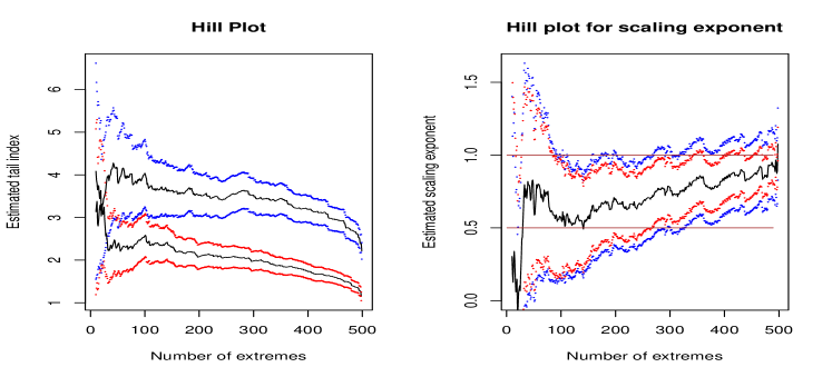
Figure 1: Exponential AR($1$) model with $\phi=0.5$ and $\alpha=2$. Left panel - tail index estimation for the original data and products. Right panel: estimation of $\kappa_{1}$ along with two types of confidence intervals. The horizontal lines indicate the true values and 1, the latter indicates extremal dependence.

Figure 2 displays boxplots for the estimates of the scaling exponent obtained from 1000 Monte Carlo simulations, for selected choices of the number of order statistics.

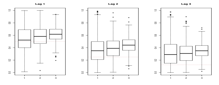
Figure 2: Exponential AR($1$) model with $\phi=0.5$, $\alpha=4$ and sample size $n=500$. Estimation of $\kappa_{1}$ (left panel), $\kappa_{2}$ (middle panel) and $\kappa_{3}$ (right panel) for $k=0.05n$ (left box), $k=0.1n$ (middle box), $k=0.2n$ (right box), based on 1000 repetitions.

5 Data Analysis

In this section we apply our theory to the volumes of sales of Microsoft stock prices from January 1, 2010. The data has been detrended by applying simple linear regression. There is some correlation in data and the absolute values of residuals. The estimated tail index for residuals is around 2, while for the products at lag 1, around 1.3-1.4. This indicates extremal independence, since under extremal dependence we would expect the tail of the product to be 1. The estimate of the scaling exponent returns 0.6, with the upper confidence interval clearly separated from 1. The confidence intervals were calculated under the assumption that the underlying process is EXPAR(1), described in Section 4.

Figure 3: Microsoft volumes data

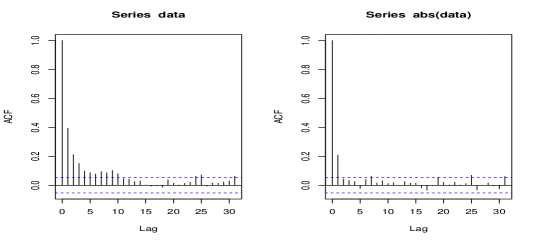
Figure 4: Microsoft volumes data: correlations

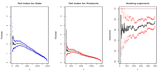
Figure 5: Microsoft volumes data: estimation of the tail index (left panel), tail index for products (mid-panel) and the conditional scaling exponent for lag 1

6 Proofs

In this section we prove our results. In Section 6.1 we prove general results on weak convergence of tail array sums; see Theorems 6.2 and 6.3. Many details are skipped, since the arguments follow basically the lines of the proofs in [KSW15], appropriately modified to incorporate the CEV assumption. These results will be applied to prove all the results of Section 2.

6.1 Convergence of tail arrays sums

For $0\leq i_{1}\leq i_{2}\in\mathbb{N}$, $0\leq j_{1}\leq j_{2}\in\mathbb{N}$ such that $i_{2}-i_{1}=j_{2}-j_{1}$ denote

$$\boldsymbol{X}_{i_{1},i_{2}}=(X_{i_{1}},\ldots,X_{i_{2}})\;,\ \ \boldsymbol{X}_{i_{1},i_{2}}/{\bf b}_{j_{1},j_{2}}(u_{n})=(X_{i_{1}}/b_{j_{1}}(u_{n}),\ldots,X_{i_{2}}/b_{j_{2}}(u_{n}))\;.$$

Let $\psi:\mathbb{R}^{h+1}\to\mathbb{R}_{+}$ be a measurable function such that

$$\lim_{\epsilon\to 0}\limsup_{x\to\infty}\frac{\mathbb{E}\left[|\psi\left(\frac{X_{0}}{x},\frac{X_{1}}{b_{1}(x)},\ldots,\frac{X_{h}}{b_{h}(x)}\right)|\mathbbm{1}{\left\{|X_{0}|\leq\epsilon x\right\}}\right]}{\overline{F}_{0}(x)}=0\;,$$ (6.1)

and either $\psi$ is bounded or there exists $\delta>0$ such that

$$\sup_{n\geq 1} \frac{\mathbb{E}\left[\psi^{2+\delta}\left(\frac{X_{0}}{u_{n}},\frac{X_{1}}{b_{1}(u_{n})},\ldots,\frac{X_{h}}{b_{h}(u_{n})}\right)\right]}{\overline{F}_{0}(u_{n})}<\infty\;.$$ (6.2)

Furthermore, we need a version of the anticlustering condition:

$$\lim_{\ell\to\infty}\limsup_{n\to\infty}\frac{1}{\overline{F}_{0}(u_{n})}\sum_{\ell<|j|\leq r_{n}}\mathbb{E}\left[\psi\left(\frac{\boldsymbol{X}_{0,h}}{{\bf b}_{0,h}(u_{n})}\right)\psi\left(\frac{\boldsymbol{X}_{j,j+h}}{{\bf b}_{0,h}(u_{n})}\right)\right]=0\;,$$ (6.3)

where $r_{n}$ is the sequence from 2 of Assumption 2.1.

Definition 6.1.

By $\mathcal{M}_{\psi}$ we denote the linear space of bounded functions $\phi:\mathbb{R}^{h+1}\to\mathbb{R}$ such that:

• $|\phi|\leq\mathrm{cst}\;\psi$ where $\mathrm{cst}$ depends on $\phi$;

• for all $j\geq 0$, the function $\boldsymbol{x}_{0,j+h}\mapsto\phi(\boldsymbol{x}_{j,j+h})$ is almost surely continuous with respect to $\boldsymbol{\mu}_{\boldsymbol{0,j+h}}$.

In this section we are interested in convergence of the tail array sums of the form

$$\widetilde{M}_{h,n}(\phi)=\frac{1}{n\overline{F}_{0}(u_{n})}\sum_{j=1}^{n-h}\phi\left(\frac{X_{j}}{u_{n}},\frac{X_{j+1}}{b_{1}(u_{n})},\ldots,\frac{X_{j+h}}{b_{h}(u_{n})}\right)\;.$$

We consider finite dimensional convergence of the process

$$\widetilde{\mathbb{M}}_{h,n}(\phi)=\sqrt{n\overline{F}_{0}(u_{n})}\left\{\widetilde{M}_{h,n}(\phi)-\mathbb{E}[\widetilde{M}_{h,n}(\phi)]\right\}$$

indexed by the set $\mathcal{M}_{\psi}$.

Theorem 6.2.

Let $\{X_{j},j\in\mathbb{Z}\}$ be a strictly stationary regularly varying sequence such that Assumption 1.1 holds with extremal independence at all lags and that Assumption 2.1 is satisfied. Let $\psi$ be a measurable function such that (6.1), (6.3) hold and either $\psi$ is bounded or there exists $\delta\in(0,1]$ such that (6.2) and

$$\lim_{n\to\infty}\frac{r_{n}}{\left(n\overline{F}_{0}(u_{n})\right)^{{\delta/2}}}=0\;$$ (6.4)

hold. Then

$$\left\{\widetilde{\mathbb{M}}_{h,n}(\phi)=\sqrt{n\overline{F}_{0}(u_{n})}\left\{\widetilde{M}_{h,n}(\phi)-\mathbb{E}[\widetilde{M}_{h,n}(\phi)]\right\},\phi\in\mathcal{M}_{\psi}\right\}\stackrel{{\scriptstyle\mbox{\small\tiny fi.di.}}}{{\to}}\left\{\mathbb{M}_{h}(\phi),\phi\in\mathcal{M}_{\psi}\right\}\;,$$

where $\mathbb{M}_{h}$ is a Gaussian process indexed by $\mathcal{M}_{\psi}$ with covariance function $(\phi,\varphi)\mapsto\boldsymbol{\mu}_{0,h}(\phi\varphi)$.

In Lemma 6.4 we will justify that under (6.1) the limit

$$\boldsymbol{\mu}_{0,h}(\phi)=\lim_{n\to\infty}\mathbb{E}[\widetilde{M}_{h,n}(\phi)]$$

is finite for $\phi\in\mathcal{M}_{\psi}$. This allows us to consider weak convergence of the process

$$\mathbb{M}_{h,n}(\phi)=\sqrt{n\overline{F}_{0}(u_{n})}\left\{\widetilde{M}_{h,n}(\phi)-\boldsymbol{\mu}_{0,h}(\phi)\right\}$$

indexed by a subset of $\mathcal{M}_{\psi}$. Let $\mathcal{G}\subseteq\mathcal{M}_{\psi}$ be equipped with a semi-metric $\rho_{h}$. The following result mimics Theorem 2.4 in [KSW15] which in turn is an adaptation of [vdVW96, Theorem 2.11.1]. Hence, it is stated without a proof.

Theorem 6.3.

Let $\{X_{j},j\in\mathbb{Z}\}$ be a strictly stationary regularly varying sequence such that Assumption 1.1 holds with extremal independence at all lags. Suppose that assumptions of Theorem 6.2 are satisfied. If moreover

1. $\mathcal{G}$ is pointwise separable;

2. the envelope function $\Phi_{\mathcal{G}}=\sup_{\phi\in\mathcal{G}}|\phi|$ is in $\mathcal{M}_{\psi}$;

3. $\mathcal{G}$ is a VC subgraph class or a finite union of such classes;

4. $(\mathcal{G},\rho_{h})$ is totally bounded;

5. for every sequence $\{\delta_{n}\}$ which decreases to zero,

   $$\limsup_{n\to\infty}\sup_{\phi,\varphi\in\mathcal{G}\atop\rho_{h}(\phi,\varphi)\leq\delta_{n}}\frac{\mathbb{E}\left[\left\{\phi\left(\frac{\boldsymbol{X}_{0,h}}{{\bf b}_{0,h}(u_{n})}\right)-\varphi\left(\frac{\boldsymbol{X}_{0,h}}{{\bf b}_{0,h}(u_{n})}\right)\right\}^{2}\right]}{\overline{F}_{0}(u_{n})}=0\;,$$ (6.5)

then

$$\widetilde{\mathbb{M}}_{h,n}(\phi)=\sqrt{n\overline{F}_{0}(u_{n})}\left\{\widetilde{M}_{h,n}(\phi)-\mathbb{E}[\widetilde{M}_{h,n}(\phi)]\right\}\Rightarrow\mathbb{M}_{h}(\phi)$$

in $\ell^{\infty}(\mathcal{G})$. If moreover

$$\lim_{n\to\infty}\sup_{\phi\in\mathcal{G}}\sqrt{n\overline{F}_{0}(u_{n})}|\mathbb{E}[\widetilde{M}_{h,n}(\phi)]-\boldsymbol{\mu}_{0,h}(\phi)|=0\;,$$ (6.6)

then

$$\mathbb{M}_{h,n}(\phi)=\sqrt{n\overline{F}_{0}(u_{n})}\left\{\widetilde{M}_{h,n}(\phi)-\boldsymbol{\mu}_{0,h}(\phi)\right\}\Rightarrow\mathbb{M}_{h}(\phi)$$

in $\ell^{\infty}(\mathcal{G})$.

The proof of Theorem 6.2 will be prefaced by several lemmas. For brevity, write

$$V_{j,n}(\phi) =\phi\left(\frac{X_{j}}{u_{n}},\frac{X_{j+1}}{b_{1}(u_{n})},\ldots,\frac{X_{j+h}}{b_{h}(u_{n})}\right)\;,\ \ S_{n}(\phi)=\sum_{j=1}^{r_{n}}V_{j,n}(\phi)\;.$$

Lemma 6.4.

Let Assumption 1.1 hold with extremal independence at all lags. Let $\psi$ be a measurable function such that (6.1) holds and either $\psi$ is bounded or (6.2) holds. Then, for all $\phi\in\mathcal{M}_{\psi}$ we have $\boldsymbol{\mu}_{0,h}(\phi^{2})<\infty$ and

$$\lim_{n\to\infty}\frac{\mathbb{E}[V_{0,n}^{2}(\phi)]}{\mathbb{P}(|X_{0}|>u_{n})}=\boldsymbol{\mu}_{\boldsymbol{0,h}}(\phi^{2})=\int_{0}^{\infty}\mathbb{E}[\phi^{2}(sW_{0},s^{\kappa_{1}}W_{1},\ldots,s^{\kappa_{h}}W_{h})]\alpha s^{-\alpha-1}\mathrm{d}s\;.$$ (6.7)

Moreover, for all $j\not=0$ and $\phi,\varphi\in\mathcal{M}_{\psi}$,

$$\lim_{n\to\infty}\frac{1}{\overline{F}_{0}(u_{n})}\mathbb{E}[V_{0,n}(\phi)V_{j,n}(\varphi)]=0\;.$$

Proof.

The proof of the first part is similar to [KS15, Proposition 2].

Assume that $\psi$ is bounded. For $\epsilon>0$, we write

$$\frac{1}{\overline{F}_{0}(u_{n})}\mathbb{E}[|V_{0,n}^{2}(\phi)|] =\frac{1}{\overline{F}_{0}(u_{n})}\mathbb{E}[|V_{0,n}^{2}(\phi)|\mathbbm{1}{\left\{|X_{0}|>\epsilon u_{n}\right\}}]+\frac{1}{\overline{F}_{0}(u_{n})}\mathbb{E}[|V_{0,n}^{2}(\phi)|\mathbbm{1}{\left\{|X_{0}|\leq\epsilon u_{n}\right\}}]\;.$$

By vague convergence and boundedness of $\phi$ the first expression on the right hand side converges to $\boldsymbol{\mu}_{\boldsymbol{0,h}}(\phi^{2}\mathbbm{1}{\left\{|y_{0}|>\epsilon\right\}})<\infty$. Application of (6.1) implies that $\boldsymbol{\mu}_{\boldsymbol{0,h}}(\phi^{2})$ is finite.

If $\psi$ is unbounded, then then for all $A>0$, applying Markov and Hölder inequalities, we obtain

$$\lim_{A\to\infty}\limsup_{n\to\infty}\frac{\mathbb{E}[V_{0,n}^{2}(\phi)\mathbbm{1}{\left\{|V_{0,n}(\phi)|>A\right\}}]}{\overline{F}_{0}(u_{n})}\leq\lim_{A\to\infty}\mathrm{cst}\cdot A^{-\delta/2}\sup_{n\geq 1}\frac{\mathbb{E}[|V_{0,n}(\phi)|^{2+\delta}]}{\overline{F}_{0}(u_{n})}=0\;.$$

Thus, we can split $V_{0,n}(\phi)$ as $V_{0,n}(\phi)\mathbbm{1}{\left\{|V_{0,n}(\phi)\leq A|\right\}}+V_{0,n}(\phi)\mathbbm{1}{\left\{|V_{0,n}(\phi)>A|\right\}}$ and apply the truncation argument.

As for the second part, thanks to the truncation argument, we can consider bounded functions $\phi,\varphi\in\mathcal{M}_{\psi}$. We have

$$\lim_{n\to\infty}\frac{\mathbb{E}[V_{0,n}(\phi)V_{j,n}(\varphi)]}{\overline{F}_{0}(u_{n})} =\lim_{n\to\infty}\frac{\mathbb{E}[V_{0,n}(\phi)V_{j,n}(\varphi)\mathbbm{1}{\left\{|X_{0}|\wedge|X_{j}|>\epsilon u_{n}\right\}}]}{\overline{F}_{0}(u_{n})}$$ (6.8)

$$\phantom{=}+\lim_{n\to\infty}\frac{\mathbb{E}[V_{0,n}(\phi)V_{j,n}(\varphi)\mathbbm{1}{\left\{|X_{0}|\wedge|X_{j}|\leq\epsilon u_{n}\right\}}]}{\overline{F}_{0}(u_{n})}\;.$$ (6.9)

The term in (6.8) vanishes, for each $\epsilon>0$, by boundedness of $\varphi,\phi$ and extremal independence. The term in (6.9) is bounded by

$$\lim_{n\to\infty}\frac{1}{\overline{F}_{0}(u_{n})}\left\{\|\varphi\|_{\infty}\mathbb{E}[V_{0,n}(\phi)\mathbbm{1}{\left\{|X_{0}|\leq\epsilon u_{n}\right\}}]+\|\phi\|_{\infty}\mathbb{E}[V_{0,n}(\varphi)\mathbbm{1}{\left\{|X_{0}|\leq\epsilon u_{n}\right\}}]\right\}$$

and hence vanishes as $\epsilon\to 0$ by (6.1). ∎

Lemma 6.5.

Let Assumption 1.1 hold with extremal independence at all lags and Assumption 2.1 hold. Let $\psi$ be a measurable function such that (6.1), (6.3) hold and either $\psi$ is bounded or (6.2) holds. Then, for all $\phi,\varphi\in\mathcal{M}_{\psi}$,

$$\lim_{n\to\infty}\frac{\mathbb{E}\left[S_{n}(\phi)S_{n}(\varphi)\right]}{r_{n}\overline{F}_{0}(u_{n})} =\boldsymbol{\mu}_{0,h}(\phi\varphi)\;,$$

and

$$\lim_{n\to\infty}\frac{\mathrm{cov}\left(S_{n}(\phi),S_{n}(\varphi)\right)}{r_{n}\mathbb{P}(|X_{0}|>u_{n})}=\boldsymbol{\mu}_{\boldsymbol{0,h}}(\phi\varphi)\;.$$

Proof.

By stationarity we can write, for $\ell\geq 1$,

$$\frac{\mathbb{E}[S_{n}(\phi)S_{n}(\varphi)]}{r_{n}\overline{F}_{0}(u_{n})}=\sum_{j=-\ell}^{\ell}\left(1-\frac{|j|}{r_{n}}\right)\frac{\mathbb{E}[V_{0,n}(\phi)V_{j,n}(\varphi)]}{\overline{F}_{0}(u_{n})}+O\left(\sum_{j=\ell+1}^{r_{n}}\frac{\mathbb{E}[V_{0,n}(\phi)V_{j,n}(\varphi)]}{\overline{F}_{0}(u_{n})}\right)\;.$$

Since $V_{0,n}(\phi)V_{0,n}(\varphi)=V_{0,n}(\phi\varphi)$, Lemma 6.4 shows that the term on the right hand side converges to $\boldsymbol{\mu}_{0,h}(\phi\varphi)$. The second term vanishes by assumption (6.3), upon letting $n\to\infty$ and then $\ell\to\infty$.

Finally, by Assumption 2.1,

$$\frac{1}{\overline{F}_{0}(u_{n})}\sum_{j=1}^{r_{n}}\mathbb{E}[V_{0,n}(\phi)]\mathbb{E}[V_{j,n}(\varphi)]=\left(\frac{\mathbb{E}[V_{0,n}(\phi)]}{\overline{F}_{0}(u_{n})}\right)^{2}r_{n}\overline{F}_{0}(u_{n})\to 0$$

and hence the result for the covariances follows. ∎

The next result can be proven along the same lines as of [KSW15, Lemmas 3.6-3.7]. In case of unbounded functions, we need additionally (6.4).

Lemma 6.6.

Let Assumption 1.1 hold with extremal independence at all lags and Assumption 2.1 hold. Let $\psi$ be a measurable function such that (6.1), (6.3) hold and either $\psi$ is bounded or there exists $\delta\in(0,1]$ such that (6.2) and (6.4) hold. Then

$$\lim_{n\to\infty}\frac{\mathbb{E}\left[S_{n}^{2}(\phi)\mathbbm{1}{\left\{|S_{n}(\phi)|>\delta\sqrt{n\overline{F}_{0}(u_{n})}\right\}}\right]}{r_{n}\overline{F}_{0}(u_{n})}=0\;.$$ (6.10)

Proof of Theorem 6.2.

Define $m_{n}=[n/r_{n}]$ and let $\{X_{n,i}^{\dagger},1\leq i\leq m_{n},n\geq 1\}$ be a triangular array of random variables such that the blocks $\{X_{(i-1)r_{n}+1}^{\dagger},\dots,X_{ir_{n}}^{\dagger}\}$ are independent and each have the same distribution as the original stationary blocks, i.e. the same distribution as $(X_{1},\dots,X_{r_{n}})$ by stationarity of the original sequence. For $i=1,\ldots,m_{n}$, define

$$V_{j,n}^{\dagger}(\phi) =\phi\left(\frac{X_{j}^{\dagger}}{u_{n}},\frac{X_{j+1}^{\dagger}}{b_{1}(u_{n})},\ldots,\frac{X_{j+h}^{\dagger}}{b_{h}(u_{n})}\right)\;,\ \ S_{n,i}^{\dagger}(\phi)=\sum_{j=(i-1)r_{n}+1}^{ir_{n}}V_{j,n}^{\dagger}(\phi)\;,$$

Arguing as in the proof of [DR10, Theorem 2.8] or [KSW15], the $\beta$-mixing property and the rate condition (2.2) implies that it suffices to prove weak convergence of the process

$$\widetilde{\mathbb{M}}_{h,n}^{\dagger}(\phi)=\{n\overline{F}_{0}(u_{n})\}^{-1/2}\sum_{i=1}^{m_{n}}\left\{S_{n,i}^{\dagger}(\phi)-\mathbb{E}[S_{n,i}^{\dagger}(\phi)]\right\}\;,$$

along with the appropriate bias condition. In the first step we show existence of the limiting covariance. For $\phi,\varphi$ we have

$$\frac{1}{\overline{F}_{0}(u_{n})}\sum_{j=1}^{r_{n}}\mathbb{E}[V_{0,n}(\phi)]\mathbb{E}[V_{j,n}(\varphi)]=\left(\frac{\mathbb{E}[V_{0,n}(\phi)]}{\overline{F}_{0}(u_{n})}\right)\left(\frac{\mathbb{E}[V_{0,n}(\varphi)]}{\overline{F}_{0}(u_{n})}\right)r_{n}\overline{F}_{0}(u_{n})\to 0\;,$$

by (6.7) and (2.3). Application of Lemma 6.5 yields the limiting covariance:

$$\lim_{n\to\infty}\mathrm{cov}\left(\widetilde{\mathbb{M}}_{h,n}^{\dagger}(\phi),\widetilde{\mathbb{M}}_{h,n}^{\dagger}(\varphi)\right)=\boldsymbol{\mu}_{0,h}(\phi\varphi)\;.$$

Lemma 6.6 finishes the proof. ∎

6.2 Proof of Theorem 2.5

We only consider the case of extremal independence, since the extremally dependent case can be concluded directly from [KSW15]. Let $s_{0}\in(0,1)$. We apply the results of Section 6.1 to the function $\psi(x_{0},\ldots,x_{h})=\mathbbm{1}{\left\{|x_{0}|>s_{0}\right\}}$ and the class $\mathcal{G}_{0}=\{\phi_{s,y}:(x_{0},\ldots,x_{h})\to\mathbbm{1}{\left\{|x_{0}|>s,x_{h}\leq y\right\}},s\geq s_{0},y\in\mathbb{R}\}$. Then

$$\widetilde{\mathbb{I}}_{h,n}(s,y)=\widetilde{\mathbb{M}}_{h,n}(\phi_{s,y})\;,\ \ \mathbb{I}_{h,n}(s,y)=\mathbb{M}_{h,n}(\phi_{s,y})\;.$$ (6.11)

We need to check assumptions (6.1)-(6.3):

• Condition (6.1) trivially holds since its right hand side vanishes whenever $\epsilon\in(0,s_{0})$;

• Condition (6.3) for the function $\psi$ is implied by the anticlustering condition (2.5) of Assumption 2.2;

Since Assumptions 1.1 and 2.1 are already assumed in Theorem 2.5, by Theorem 6.2, the finite dimensional distributions of

$$\sqrt{n\overline{F_{0}}(u_{n})}\{\widetilde{I}_{h,n}(s,y)-\mathbb{E}[\widetilde{I}_{h,n}(s,y)]\}$$

converge to those of ${\mathbb{I}}_{h}$.

To prove tightness, we apply Theorem 6.3. Condition (6.6) reduces to (2.6). It remains to verify i-v. Define the semi-metric $\rho_{h}$ on $(0,\infty)\times\mathbb{R}$ by

$$\rho_{h}((s,y),(t,z))=|s-t|+|\Psi_{h}(y)-\Psi_{h}(z)|\;.$$ (6.12)

This also defines the semi-metric on $\mathcal{G}_{0}$. The class is clearly pointwise separable and the envelope function is $\mathbbm{1}{\left\{(s_{0},\infty)\times\mathbb{R}^{h}\right\}}\in\mathcal{M}_{\psi}$. Also, the class of indicators of the sets $(s,\infty)\times(-\infty,y]$ is a VC class of index 2. The proof of iv-v follows the same lines as that of [KSW15, Theorem 2.11]. It remains to identify the limiting Gaussian process. For $0<s<t$ and $y,z\in\mathbb{R}$, we have

$$\mathrm{cov}({\mathbb{M}}(\phi_{s,y}),{\mathbb{M}}(\phi_{t,z})) =\boldsymbol{\mu}_{0,h}(\phi_{s,y}\phi_{t,z})=t^{-\alpha}\Psi_{h}(t^{-\kappa_{h}}(y\wedge z))\;.$$

This finishes the proof.

6.3 Central limit theorem for the conditional mean

We state another corollary to Theorem 6.3. For $s>0$, set $\psi_{s}(x_{0},\ldots,x_{h})=|x_{h}|\mathbbm{1}{\left\{|x_{0}|>s\right\}}$ and define the class

$$\mathcal{G}_{1}=\{\psi_{s},s\geq s_{0}\}\;.$$

Then,

$$\mathbb{M}_{h,n}(\psi_{s})=\sqrt{n\overline{F}_{0}(u_{n})}\left\{\frac{1}{n\overline{F}_{0}(u_{n})}\sum_{j=1}^{n-h}\frac{|X_{j+h}|}{b_{h}(u_{n})}\mathbbm{1}{\left\{|X_{j}|>u_{n}s\right\}}-\boldsymbol{\mu}_{0,h}(\psi_{s})\right\}\;.$$ (6.13)

By the homogeneity property (1.5) and the assumption $\int_{-\infty}^{\infty}|y|\,\Psi_{h}(\mathrm{d}y)=1$, we have

$$\boldsymbol{\mu}_{0,h}(\psi_{s})=s^{\kappa_{h}-\alpha}\;.$$ (6.14)

Corollary 6.7.

Let $\{X_{j},j\in\mathbb{Z}\}$ be a strictly stationary regularly varying sequence such that Assumption 1.1 holds with extremal independence at all lags and that Assumption 2.1 is satisfied. Assume that Assumptions 2.2, 2.3 and 2.6 and (6.4) hold. Then

$$\mathbb{M}_{h,n}\stackrel{{\scriptstyle\mbox{\tiny\rm w}}}{{\longrightarrow}}{\mathbb{M}}_{h}\;,\ \mbox{ in }\ell^{\infty}(\mathcal{G}_{0}\cup\mathcal{G}_{1})\;.$$

Proof.

Let $s_{0}\in(0,1)$. We apply the results of Section 6.1. We need to check the assumptions (6.1)-(6.3):

• Condition (6.1) holds trivially for $\psi(x_{0},\ldots,x_{h})=|x_{h}|\mathbbm{1}{\left\{|x_{0}|>s_{0}\right\}}$.

• (2.8) of Assumption 2.6 implies (6.2).

• (2.9) of Assumption 2.6 implies (6.3).

For tightness, we apply Theorem 6.3. Condition (6.6) reduces to (2.10). It remains to verify i-v. The class $\mathcal{G}_{1}$ is separable and linearly ordered, hence VC-subgraph class. The envelope function $|x_{h}|\mathbbm{1}{\left\{|x_{0}|>s_{0}\right\}}$ belongs to $\mathcal{G}_{1}$.

Define the semi-metric $\rho_{h}$ on $\mathcal{G}_{1}$ by

$$\rho_{h}(\psi_{s},\psi_{t})=\mathbb{E}[Y_{0}^{2}W_{h}^{2}\mathbbm{1}{\left\{Y_{0}\in(s,t]\right\}}]\;.$$ (6.15)

Since Assumption 2.6 implies $\alpha>2$ we have for $s<t$,

$$\rho_{h}(\psi_{s},\psi_{t})=\frac{\alpha}{\alpha-2}\mathbb{E}[W_{h}^{2}](s^{-\alpha+2}-t^{-\alpha+2})\leq\mathrm{cst}(t-s)\;.$$

Hence, $(\mathcal{G}_{1},\rho_{h})$ is totally bounded. Moreover, by regular variation and the uniform convergence theorem, the convergence

$$\lim_{n\to\infty}\frac{1}{b_{h}^{2}(u_{n})\overline{F}_{0}(u_{n})}\mathbb{E}[X_{h}^{2}\left(\mathbbm{1}{\left\{X_{0}>su_{n}\right\}}-\mathbbm{1}{\left\{X_{0}>tu_{n}\right\}}\right)]=\frac{\alpha}{\alpha-2}\mathbb{E}[W_{h}^{2}](s^{-\alpha+2}-t^{-\alpha+2})$$

is uniform on compact sets of $(0,\infty)$. Hence, v holds. The joint convergence holds by applying Theorem 2.5 and considering the class $\mathcal{G}=\mathcal{G}_{0}\cup\mathcal{G}_{1}$. ∎

6.4 Proof of Corollaries 2.7 and 2.9

Proof of Corollary 2.7.

Set $\mathsf{T}_{n}(s)=k^{-1}\sum_{j=1}^{n}\mathbbm{1}{\left\{|X_{j}|>u_{n}s\right\}}$. By Corollary 6.7 and Vervaat’s lemma [Ver72], we obtain the joint convergence

$$\left\{\mathbb{M}_{h,n}(\psi_{s}),\mathbb{I}_{h,n}(s,y),\sqrt{k}\left(\mathsf{T}_{n}(s)-s^{-\alpha}\right),\sqrt{k}\left(u_{n}^{-1}|X|_{(n:k)}-1\right)\right\}\\ \stackrel{{\scriptstyle\mbox{\tiny\rm w}}}{{\longrightarrow}}\left\{\mathbb{M}_{h}(\psi_{s}),\mathbb{M}_{h}(\phi_{s,y}),\mathbb{M}_{h}(\phi_{s,\infty}),\alpha^{-1}\mathbb{M}_{h}(\phi_{1,\infty})\right\}\;.$$ (6.16)

Write $\xi_{n}=u_{n}^{-1}|X|_{(n:k)}$ and note that the above weak convergence implies that $\xi_{n}\to 1$ in probability. Note that by (6.14), we have

$$\boldsymbol{\mu}_{0,h}(\psi_{\xi_{n}})=\xi_{n}^{\kappa_{h}-\alpha}\;.$$

In view of this identity and (6.13), we have

$$\sqrt{k}\left(\frac{\widehat{b}_{h,n}}{b_{h}(u_{n})}-1\right) =\mathbb{M}_{h,n}(\psi_{\xi_{n}})+\sqrt{k}\left\{\xi_{n}^{\kappa_{h}-\alpha}-1\right\}\;.$$ (6.17)

Thus,

$$\sqrt{k}\left(\frac{\widehat{b}_{h,n}}{b_{h}(u_{n})}-1\right) \stackrel{{\scriptstyle\mbox{\tiny\rm d}}}{{\longrightarrow}}\mathbb{M}_{h}({\psi_{1}})+\alpha^{-1}(\kappa_{h}-\alpha)\mathbb{M}_{h}(\phi_{1,\infty})\;.$$

The process $\mathbb{W}$ defined by $\mathbb{W}(u)=\mathbb{M}_{h}(\phi_{1,\Psi_{h}^{-1}(u)})$ is a standard Brownian motion and $\mathbb{B}(u)=\mathbb{W}(u)-u\mathbb{W}(1)$ is a standard Brownian bridge. Therefore,

$$\mathbb{M}_{h}({\psi_{1}})=\int_{0}^{1}|\Psi_{h}^{-1}(u)|\mathbb{W}(\mathrm{d}u)\;.$$

By assumption, we have

$$\int_{0}^{1}|\Psi_{h}^{-1}(u)|\mathrm{d}u=\int_{-\infty}^{\infty}|y|\Psi_{h}(\mathrm{d}y)=1\;,$$

thus $\mathbb{M}_{h}({\psi_{1}})-\mathbb{M}_{h}(\phi_{1,\infty})=\int_{0}^{1}| \Psi_{h}^{-1}(u)|\mathbb{B}(\mathrm{d}u)$. ∎

Proof of Corollary 2.9.

Writing $\theta_{n}=b_{h}^{-1}(u_{n})\widehat{b}_{h,n}$, we have

$$\sqrt{k}\left\{\widehat{\Psi}_{h,n}(y)-\Psi_{h}(y)\right\} =\sqrt{k}\left\{\widetilde{I}_{h,n}\left(\frac{X_{(n:n-k)}}{u_{n}},\frac{\widehat{b}_{h,n}}{b_{h}(u_{n})}y\right)-\Psi_{h}(y)\right\}$$

$$=\mathbb{I}_{h,n}(\xi_{n},\theta_{n}y)+\sqrt{k}\left(\xi_{n}^{-\alpha}\Psi_{h}(\xi_{n}^{-\kappa_{h}}\theta_{n}y)-\Psi_{h}(y)\right)\;.$$ (6.18)

By Corollary 2.7, $\xi_{n}\stackrel{{\scriptstyle\mbox{\small\tiny p}}}{{\longrightarrow}}1$ and $\theta_{n}\stackrel{{\scriptstyle\mbox{\small\tiny p}}}{{\longrightarrow}}1$. Hence, the first term in (6.18) converges to $\mathbb{M}_{h}(\phi_{1,y})$. The delta method implies that the limiting behaviour of the second term in (6.18) is the same as that of

$$\sqrt{k}\Psi_{h}(y)\left\{\xi_{n}^{-\alpha}-1\right\}+\xi_{n}^{-\alpha}\sqrt{k}y\Psi_{h}^{\prime}(y)\left\{\xi_{n}^{-\kappa_{h}}-1+\xi_{n}^{-\kappa_{h}}(\theta_{n}-1)\right\}\;,$$

which by Corollary 2.7 converges weakly to

$$-\Psi_{h}(y)\mathbb{M}_{h}(\phi_{1,\infty})+y\Psi_{h}^{\prime}(y)\{\mathbb{M}_{h}(\psi_{1})-\mathbb{M}_{h}(\phi_{1,\infty})\}\;.$$

Moreover, with $\mathbb{W}$ and $\mathbb{B}$ as above, we have

$$\{\mathbb{M}_{h}(\phi_{1,y})-\Psi_{h}(y) \mathbb{M}_{h}(\phi_{1,\infty}),y\in\mathbb{R}\}=\mathbb{B}\circ\Psi\;.$$

This concludes the proof. ∎

6.5 Proof of Theorem 2.13

Set $\beta_{h}=\alpha/(1+\kappa_{h})$ and $\gamma_{h}=\beta_{h}^{-1}$. At the first step we justify functional convergence of the tail empirical process based on products:

$$\sqrt{n\overline{F}_{0}(u_{n})}\left\{\frac{1}{n\overline{F}_{0}(u_{n})}\sum_{j=1}^{n-h}\mathbbm{1}{\left\{|X_{j}X_{j+h}|>\|W_{h}\|_{\beta_{h}}u_{n}b_{h}(u_{n})s\right\}}-s^{-\beta_{h}}\right\}\;.$$ (6.19)

Define $\psi(x_{0},\ldots,x_{h})=\mathbbm{1}{\left\{|x_{0}|>s_{0}\right\}}+\mathbbm{1}{\left\{\|W_{h}\|_{\beta_{h}}|x_{0}x_{h}|>s_{0}\right\}}$ and the class $\mathcal{G}=\mathcal{G}_{0}^{\prime}\cup\mathcal{G}_{1}^{\prime}$ with

$$\mathcal{G}_{0}^{\prime} =\{\mathcal{I}_{s}:(x_{0},\ldots,x_{h})\to\mathbbm{1}{\left\{|x_{0}|>s\right\}},s\geq s_{0}\}\;,$$

$$\mathcal{G}_{1}^{\prime} =\{\varphi_{s}:(x_{0},\ldots,x_{h})\to\mathbbm{1}{\left\{|x_{0}x_{h}|>s\|W_{h}\|_{\beta_{h}}\right\}},s\geq s_{0}\}\;.$$

With this notation the process defined in (6.19) can be written as $\mathbb{M}_{h,n}(\varphi_{s})$. Similarly, the tail empirical process of $X_{j}$’s can be written as $\mathbb{M}_{h,n}(\mathcal{I}_{s})$:

$$\mathbb{M}_{h,n}(\mathcal{I}_{s})=\sqrt{n\overline{F}_{0}(u_{n})}\left\{\frac{1}{n\overline{F}_{0}(u_{n})}\sum_{j=1}^{n}\mathbbm{1}{\left\{|X_{j}|>u_{n}s\right\}}-s^{-\alpha}\right\}\;.$$

We note that $\mathcal{G}_{0}^{\prime}\subseteq\mathcal{G}_{0}$, where $\mathcal{G}_{0}$ was defined in the proof of Theorem 2.5 and $\mathcal{I}_{s}=\phi_{s,\infty}$. Assumptions (2.15) and (2.18) imply (6.1) and (6.3) for the class $\mathcal{G}_{1}^{\prime}$. The bias condition (6.6) is implied by (2.21). Therefore, by Theorem 6.2, the finite dimensional distributions of $\mathbb{M}_{h,n}$ converge to those of $\mathbb{M}_{h}$ of $\mathcal{G}_{1}^{\prime}$. Moreover, the envelope function of $\mathcal{G}$ is $\psi$. Furthermore,

• The class $\mathcal{G}$ is the union of two linearly ordered classes, hence is a VC subgraph class.

• We consider the metric $\rho_{h}$ on $\mathcal{G}$ induced by the covariance, that is for $\phi,\varphi\in\mathcal{G}$,

  $$\rho_{h}(\phi,\varphi)=\sqrt{\mathrm{var}(\mathbb{M}_{h}(\phi)-\mathbb{M}_{h}(\varphi))}\;.$$

  The metric $\rho_{h}$ restricted to $\mathcal{G}_{0}^{\prime}$ and $\mathcal{G}_{1}^{\prime}$ respectively becomes

  $$\rho_{h}(\mathcal{I}_{s},\mathcal{I}_{t})=\sqrt{|s^{-\alpha}-t^{-\alpha}|}\;,\ \ \rho_{h}(\varphi_{s},\varphi_{t}) =\sqrt{|s^{-\beta_{h}}-t^{-\beta_{h}}|}\;.$$

  Thus it easily seen that both $\mathcal{G}_{0}^{\prime}$ and $\mathcal{G}_{1}^{\prime}$ are totally bounded for the metric $\rho_{h}$. This means that Condition iv holds.

• By regular variation, the convergence

  $$\lim_{n\to\infty}\frac{1}{\overline{F}_{0}(u_{n})}\mathbb{E}[\mathbbm{1}{\left\{|X_{0}X_{h}|\in u_{n}b_{h}(u_{n})(s,t]\right\}}]=\rho_{h}^{2}(\varphi_{s},\varphi_{t})$$

  is uniform with respect to $s,t\in[s_{0},\infty)$ (see [BGT89, Theorem 1.5.2]). Therefore, v holds on $\mathcal{G}_{1}^{\prime}$.

Thus we have proved that

$$\mathbb{M}_{h,n}\implies\mathbb{M}_{h}\;,\ \mbox{ in }\ell^{\infty}(\mathcal{G})\;.$$

Recall that $\xi_{n}=|X|_{(n:n-k)}/u_{n}$. Set $V_{j}=|X_{j}X_{j+h}|$ and $v_{n}=u_{n}b(u_{n})\|W_{h}\|_{\beta_{h}}$. Define

$$\zeta_{n}=V_{(n:n-k)}/v_{n}\;.$$

As a consequence of the functional convergence and Vervaat’s Lemma, we obtain

$$\left(\mathbb{M}_{h,n},\sqrt{k}(\xi_{n}-1),\sqrt{k}(\zeta_{n}-1)\right)\implies(\mathbb{M}_{h},\gamma\mathbb{M}_{h}(\mathcal{I}_{1}),\gamma_{h}\mathbb{M}_{h}(\varphi_{1}))\;;$$ (6.20)

By elementary algebra and Fubini’s theorem, we have

$$\sqrt{k}(\hat{\gamma}-\gamma) =\int_{1}^{\infty}\mathbb{M}_{h,n}(\mathcal{I}_{s})\frac{\mathrm{d}s}{s}+\int_{\xi_{n}}^{1}\mathbb{M}_{h,n}(\mathcal{I}_{s})\frac{\mathrm{d}s}{s}+\gamma\sqrt{k}(\xi_{n}^{-1/\gamma}-1)\;,$$

$$\sqrt{k}(\hat{\gamma}_{h}-\gamma_{h}) =\int_{1}^{\infty}\mathbb{M}_{h,n}(\varphi_{s})\frac{\mathrm{d}s}{s}+\int_{\zeta_{n}}^{1}\mathbb{M}_{h,n}(\varphi_{s})\frac{\mathrm{d}s}{s}+\gamma_{h}\sqrt{k}(\zeta_{n}^{-1/\gamma_{h}}-1)\;.$$

The middle term of both expansions is $o_{P}(1)$. The last terms are dealt with by Slutsky’s theorem and (6.20):

$$\left(\sqrt{k}(\xi_{n}^{-1/\gamma}-1),\sqrt{k}(\zeta_{n}^{-1/\gamma_{h}}-1)\right)\implies\left(-\mathbb{M}_{h}(\mathcal{I}_{1}),-\mathbb{M}_{h}(\varphi_{1})\right)\;.$$ (6.21)

Furthermore, jointly with the previous convergences,

$$\left(\int_{1}^{\infty}\mathbb{M}_{h,n}(\mathcal{I}_{s})\frac{\mathrm{d}s}{s},\int_{1}^{\infty}\mathbb{M}_{h,n}(\varphi_{s})\frac{\mathrm{d}s}{s}\right)\implies\left(\int_{1}^{\infty}\mathbb{M}_{h}(\mathcal{I}_{s})\frac{\mathrm{d}s}{s},\int_{1}^{\infty}\mathbb{M}_{h}(\varphi_{s})\frac{\mathrm{d}s}{s}\right)\;.$$ (6.22)

Indeed, for a fixed $A>1$, we can write

$$\int_{1}^{\infty}\mathbb{M}_{h,n}(\mathcal{I}_{s})\frac{\mathrm{d}s}{s}=\int_{1}^{A}\mathbb{M}_{h,n}(\mathcal{I}_{s})\frac{\mathrm{d}s}{s}+\int_{A}^{\infty}\mathbb{M}_{h,n}(\mathcal{I}_{s})\frac{\mathrm{d}s}{s}\;,$$

$$\int_{1}^{\infty}\mathbb{M}_{h,n}(\varphi_{s})\frac{\mathrm{d}s}{s}=\int_{1}^{A}\mathbb{M}_{h,n}(\varphi_{s})\frac{\mathrm{d}s}{s}+\int_{A}^{\infty}\mathbb{M}_{h,n}(\varphi_{s})\frac{\mathrm{d}s}{s}\;.$$

By Theorem 6.3, we have

$$\left(\int_{1}^{A}\mathbb{M}_{h,n}(\mathcal{I}_{s})\frac{\mathrm{d}s}{s},\int_{1}^{A}\mathbb{M}_{h,n}(\varphi_{s})\frac{\mathrm{d}s}{s}\right)\implies\left(\int_{1}^{A}\mathbb{M}_{h}(\mathcal{I}_{s})\frac{\mathrm{d}s}{s},\int_{1}^{A}\mathbb{M}_{h}(\varphi_{s})\frac{\mathrm{d}s}{s}\right)\;.$$

Moreover, as $A\to\infty$,

$$\left(\int_{1}^{A}\mathbb{M}_{h}(\mathcal{I}_{s})\frac{\mathrm{d}s}{s},\int_{1}^{A}\mathbb{M}_{h}(\varphi_{s})\frac{\mathrm{d}s}{s}\right)\stackrel{{\scriptstyle\mbox{\small\tiny p}}}{{\longrightarrow}}\left(\int_{1}^{\infty}\mathbb{M}_{h}(\mathcal{I}_{s})\frac{\mathrm{d}s}{s},\int_{1}^{\infty}\mathbb{M}_{h}(\varphi_{s})\frac{\mathrm{d}s}{s}\right)\;.$$

Therefore, we must prove that for all $\epsilon>0$,

$$\lim_{A\to\infty}\limsup_{n\to\infty}\mathbb{P}\left(\left|\int_{A}^{\infty}\mathbb{M}_{h,n}(\mathcal{I}_{s})\frac{\mathrm{d}s}{s}\;.\right|>\epsilon\right)=0\;,$$

$$\lim_{A\to\infty}\limsup_{n\to\infty}\mathbb{P}\left(\left|\int_{A}^{\infty}\mathbb{M}_{h,n}(\varphi_{s})\frac{\mathrm{d}s}{s}\;.\right|>\epsilon\right)=0\;.$$

The proof of these bounds rely on the $\beta$ mixing property and Conditions (2.19) and (2.20). We will only prove the first one, the second being exactly similar. First note that

$$\int_{A}^{\infty}\mathsf{T}_{n}(\mathcal{I}_{s})\frac{\mathrm{d}s}{s}=\frac{1}{k}\sum_{j=1}^{n}\log_{+}(|X_{j}|/Au_{n})$$

In view of Assumption 2.1, it suffices to consider independent blocks and thus to compute the variance of one block, that is we must prove that

$$\lim_{A\to\infty}\limsup_{n\to\infty}m_{n}\mathrm{var}\left(k^{-1/2}\sum_{i=1}^{r_{n}}\log_{+}(|X_{j}|/Au_{n})\right)=0$$

Let the variance term in the previous display be denoted by $\mathcal{V}_{n}(A)$. Then,

$$\mathcal{V}_{n}(A)\leq\frac{\mathbb{E}[\log_{+}^{2}(|X_{0}|/u_{n})}{\overline{F}_{0}(u_{n})}+2\sum_{j=1}^{r_{n}}\frac{\mathbb{E}[\log_{+}(|X_{0}|/Au_{n})\log_{+}(|X_{j}|/Au_{n})]}{\overline{F}_{0}(u_{n})}\;.$$

By regular variation, extremal independence and condition (2.19), for every $\epsilon>0$, we can choose an integer $m$ such that

$$\limsup_{n\to\infty}\mathcal{V}_{n}(A) =\int_{A}^{\infty}\log^{2}(x/A)\alpha x^{-\alpha-1}\mathrm{d}x$$

$$\phantom{=}+2\limsup_{n\to\infty}\sum_{j=m+1}^{r_{n}}\frac{\mathbb{E}[\log_{+}(|X_{0}|/u_{n})\log_{+}(|X_{j}|/u_{n})]}{\overline{F}_{0}(u_{n})}$$

$$\leq A^{-\alpha}\int_{1}^{\infty}\log^{2}(y)\alpha y^{-\alpha-1}\mathrm{d}y+\epsilon\;.$$

Thus $\lim_{A\to\infty}\limsup_{n\to\infty}\mathcal{V}_{n}(A)\leq\epsilon$. Since $\epsilon$ is arbitrary, this proves the requested bound.

Combining (6.21) and (6.22), we have proved that

$$\sqrt{k}\left(\hat{\gamma}-\gamma,\hat{\gamma}_{h}-\gamma_{h}\right)\stackrel{{\scriptstyle\mbox{\tiny\rm d}}}{{\longrightarrow}}\left(\int_{1}^{\infty}\mathbb{M}_{h}(\mathcal{I}_{s})\frac{\mathrm{d}s}{s}-\mathbb{M}_{h}(\mathcal{I}_{1}),\int_{1}^{\infty}\mathbb{M}_{h}(\psi_{s})\frac{\mathrm{d}s}{s}-\mathbb{M}_{h}(\psi_{1})\right)\;.$$ (6.23)

Define the Gaussian process $\mathbb{G}$ on $(0,\infty)\times\mathbb{R}$ by $\mathbb{G}(s,y)=\mathbb{M}_{h}(\phi_{s,y})$. Then,

$$\int_{1}^{\infty}\mathbb{M}_{h}(\mathcal{I}_{s})\frac{\mathrm{d}s}{s}-\mathbb{M}_{h}(\mathcal{I}_{1}) =\int_{0}^{\infty}\int_{-\infty}^{\infty}\{\log_{+}(u)-\gamma\mathbbm{1}{\left\{u>1\right\}}\}\mathbb{G}(\mathrm{d}u\mathrm{d}v)\;,$$

$$\int_{1}^{\infty}\mathbb{M}_{h}(\varphi_{s})\frac{\mathrm{d}s}{s}-\mathbb{G}(\varphi_{1}) =\int_{0}^{\infty}\int_{-\infty}^{\infty}\{\log_{+}(u|v|)-\gamma_{h}\mathbbm{1}{\left\{u|v|>1\right\}}\}\mathbb{G}(\mathrm{d}u\mathrm{d}v)\;.$$

Write

$$\sqrt{k}(\hat{\kappa}_{h}-\kappa)=\sqrt{k}\left\{\widehat{\gamma}_{h}/\widehat{\gamma}-\gamma_{h}/\gamma\right\}=\sqrt{k}\frac{1}{\widehat{\gamma}}\left\{\widehat{\gamma}_{h}-\gamma_{h}\right\}-\sqrt{k}\frac{\gamma_{h}}{\hat{\gamma}\gamma}\left\{\widehat{\gamma}^{-1}-\gamma^{-1}\right\}\;.$$

Applying the joint convergence (6.23), Slutsky lemma and the delta method, we obtain,

$$\sqrt{k}(\hat{\kappa}_{h}-\kappa_{h})\stackrel{{\scriptstyle\mbox{\tiny\rm d}}}{{\longrightarrow}}\\ (1+\kappa_{h})\int_{0}^{\infty}\!\!\int_{-\infty}^{\infty}\left(\beta_{h}\log_{+}(u|v|)-\mathbbm{1}{\left\{u|v|>1\right\}}-\alpha\log_{+}(u)+\mathbbm{1}{\left\{u>1\right\}}\right)\mathbb{G}(\mathrm{d}u,\mathrm{d}v)\;.$$

There remains to compute the variance $\sigma^{2}$ of the limiting distribution which is Gaussian with zero mean. Setting

$$h(u,v)=\beta_{h}\log_{+}(u|v|)-\mathbbm{1}{\left\{u|v|>1\right\}}-\alpha\log_{+}(u)+\mathbbm{1}{\left\{u>1\right\}}\;,$$

and combining with (1.6) we obtain

$$\sigma^{2} =(1+\kappa_{h})^{2}\mathbb{E}\left[\int_{0}^{\infty}h^{2}(s,s^{\kappa_{h}}|W_{h}|)\alpha s^{-\alpha-1}\mathrm{d}s\right]\;.$$

Since $h^{2}(s,s^{\kappa_{h}}|W_{h}|)=0$ if $s<1$ and $s^{1+\kappa_{h}}|W_{h}|<1$, we have

$$\sigma^{2} =(1+\kappa_{h})^{2}\mathbb{E}\left[\int_{1\wedge W_{h}^{-1/(1+\kappa_{h})}}^{\infty}h^{2}(s,s^{\kappa_{h}}|W_{h}|)\alpha s^{-\alpha-1}\mathrm{d}s\right]\;.$$

Setting $A=|W_{h}|^{\beta_{h}}$ and substituting $t=s^{-\alpha}$ we obtain

$$\int_{1\wedge W_{h}^{-1/(1+\kappa_{h})}}^{\infty}h^{2}(s,s^{\kappa_{h}}|W_{h}|)\alpha s^{-\alpha-1}\mathrm{d}s=\int_{0}^{1\vee A}h^{2}(t^{-1/\alpha},t^{-\kappa_{h}/\alpha}|W_{h}|)\mathrm{d}t\;.$$

We also note that

$$h(t^{-1/\alpha},t^{-\kappa_{h}/\alpha}|W_{h}|)=\left\{\log_{+}(t^{-1}A)-\mathbbm{1}{\left\{A>t\right\}}\right\}-\left\{\log_{+}(t^{-1})-\mathbbm{1}{\left\{t<1\right\}}\right\}\;.$$

If $A<1$, then we evaluate

$$\int_{0}^{1}h^{2}(t^{-1/\alpha},t^{-\kappa_{h}/\alpha}|W_{h}|)\mathrm{d}t=A\log^{2}(A)+\int_{A}^{1}\left\{\log(t)+1\right\}^{2}\mathrm{d}t\;.$$

Since the primitive of $\left\{\log(t)+1\right\}^{2}$ is $t\log^{2}(t)+t$, the right hand side becomes $1-A$. If $A>1$, then

$$\int_{0}^{1}h^{2}(t^{-1/\alpha},t^{-\kappa_{h}/\alpha}|W_{h}|)\mathrm{d}t=\log^{2}(A)+\int_{1}^{A}\left\{\log(A)-\log(t)-1\right\}^{2}\mathrm{d}t=A-1\;.$$

Summarizing,

$$\sigma^{2}=(1+\kappa_{h})^{2}\mathbb{E}[|1-|W_{h}|^{\beta_{h}}|]\;.$$

Acknowledgements

The research of Clemonell Bilayi and Rafal Kulik was supported by the NSERC grant 210532-170699-2001. The research of Philippe Soulier was partially supported by the LABEX MME-DII.

Clemonell Bilayi-Biakana: cbilayib@uottawa.ca
University of Ottawa,
Department of Mathematics and Statistics,
585 King Edward Av.,
K1J 8J2 Ottawa, ON, Canada

Rafał Kulik: rkulik@uottawa.ca
University of Ottawa,
Department of Mathematics and Statistics,
585 King Edward Av.,
K1J 8J2 Ottawa, ON, Canada

Philippe Soulier: philippe.soulier@u-paris10.fr
Université Paris Nanterre,
Département de mathématiques et informatique,
Laboratoire MODAL’X EA3454,
92000 Nanterre, France

References

• [BGT89] Nicholas H. Bingham, Charles M. Goldie, and Jozef L. Teugels. Regular variation. Cambridge University Press, Cambridge, 1989.
• [Bra05] Richard C. Bradley. Basic properties of strong mixing conditions. A survey and some open questions. Probability Surveys, 2:107–144, 2005.
• [DJe17] Holger Drees and Anja Janß en. Conditional extreme value models: fallacies and pitfalls. Extremes, 20(4):777–805, 2017.
• [DM01] Richard A. Davis and Thomas Mikosch. Point process convergence of stochastic volatility processes with application to sample autocorrelation. Journal of Applied Probability, 38A:93–104, 2001. Probability, statistics and seismology.
• [DR10] Holger Drees and Holger Rootzén. Limit theorems for empirical processes of cluster functionals. Ann. Statist., 38(4):2145–2186, 2010.
• [DR11] Bikramjit Das and Sidney I. Resnick. Conditioning on an extreme component: model consistency with regular variation on cones. Bernoulli, 17(1):226–252, 2011.
• [Dre00] Holger Drees. Weighted approximations of tail processes for $\beta$-mixing random variables. The Annals of Applied Probability, 10(4):1274–1301, 2000.
• [Dre02] Holger Drees. Tail empirical processes under mixing conditions. In Empirical process techniques for dependent data, pages 325–342. Birkhäuser Boston, Boston, MA, 2002.
• [DSW15] Holger Drees, Johan Segers, and Michał Warchoł. Statistics for tail processes of Markov chains. Extremes, 18(3):369–402, 2015.
• [HL06] Henrik Hult and Filip Lindskog. Regular variation for measures on metric spaces. Publ. Inst. Math. (Beograd) (N.S.), 80(94):121–140, 2006.
• [HR07] Janet E. Heffernan and Sidney I. Resnick. Limit laws for random vectors with an extreme component. The Annals of Applied Probability, 17(2):537–571, 2007.
• [JD16] Anja Janssen and Holger Drees. A stochastic volatility model with flexible extremal dependence structure. Bernoulli, 22(3):1448–1490, 2016.
• [Kal17] Olav Kallenberg. Random Measures, Theory and Applications, volume 77 of Probability Theory and Stochastic Modelling. Springer-Verlag, New York, 2017.
• [KS11] Rafał Kulik and Philippe Soulier. The tail empirical process for long memory stochastic volatility sequences. Stochastic Processes and their Applications, 121(1):109 – 134, 2011.
• [KS15] Rafał Kulik and Philippe Soulier. Heavy tailed time series with extremal independence. Extremes, 18:273–299, 2015.
• [KSW15] Rafał Kulik, Philippe Soulier, and Olivier Wintenberger. Practical conditions for weak convergence of tail empirical processes. arxiv:1511.04903, 2015.
• [LRR14] Filip Lindskog, Sidney I. Resnick, and Joyjit Roy. Regularly varying measures on metric spaces: hidden regular variation and hidden jumps. Probability Surveys, 11:270–314, 2014.
• [MR13] Thomas Mikosch and Mohsen Rezapour. Stochastic volatility models with possible extremal clustering. Bernoulli, 19(5A):1688–1713, 2013.
• [Roo09] Holger Rootzén. Weak convergence of the tail empirical process for dependent sequences. Stoch. Proc. Appl., 119(2):468–490, 2009.
• [vdVW96] Aad W. van der Vaart and Jon A. Wellner. Weak convergence and empirical processes. Springer, New York, 1996.
• [Ver72] Wim Vervaat. Functional central limit theorems for processes with positive drift and their inverses. Z. Wahrscheinlichkeitstheorie und Verw. Gebiete, 23:245–253, 1972.