A nonparametric ensemble binary classifier and its statistical properties

Abstract

In this work, we propose an ensemble of classification trees (CT) and artificial neural networks (ANN). Several statistical properties including universal consistency and upper bound of an important parameter of the proposed classifier are shown. Numerical evidence is also provided using various real life data sets to assess the performance of the model. Our proposed nonparametric ensemble classifier doesn’t suffer from the “curse of dimensionality” and can be used in a wide variety of feature selection cum classification problems. Performance of the proposed model is quite better when compared to many other state-of-the-art models used for similar situations.

1 Introduction

Distribution-free classification models are specially used in the fields of statistics and machine learning since more than forty years now, mainly for their accuracy and ability to deal with high dimensional features and complex data structures. Two such models are CT and ANN. Both have the ability to model arbitrary decision boundaries. CT is found to be robust when limited data are available unlike ANN. But decision trees are high variance estimators and greedy in nature [1] whereas neural networks are universal approximators [2]. More powerful ANN has many free tuning parameters and risk of over-fitting for small data sets. To utilize the positive aspects of these two powerful models, theoretical frameworks for combining both classifiers are often used jointly to make decisions. The ultimate goal of designing classification models is to achieve best possible performance in terms of accuracy measures for the task at hand. This objective led researchers to create efficient hybrid models and prove their statistical properties to make their best use. Mapping tree based models to neural networks allows exploiting the former to initialize the latter. Parameter optimization within ANN framework will yield a model that is intermediate between CT and ANN as found in some literatures [3, 4]. Tsai neural tree model [5] uses the idea of splitting the parameter space into areas by CT and builds in each of the areas a locally specialized ANN model [6]. In deep neural tree model [7], a decision tree provides the final prediction and it differs from conventional CT by introducing a global optimization of split and leaf node parameters using ANN. But the major disadvantages of these algorithms are slow training, having many tuning parameters, easy sticking on local minima and poor robustness [5]. All these hybrid models are empirically shown to be useful in solving real life problems, but the theoretical results are yet to be proved for many of them.

On the theoretical side, the literature is less conclusive, and regardless of their use in practical problems of classification, little is known about the statistical properties of these models. The most celebrated theoretical result has given the general sufficient conditions for almost-sure $L_{1}$-consistency of histogram-based classification and data-driven density estimates [8]. In case of neural networks, it is theoretically proven that if a one hidden layered (1HL) neural network is trained with appropriately chosen number of neurons to minimize the empirical risk on the training data, then it results in a universally consistent classifier [9, 10]. Devroye et al. [11] have theoretically shown that there is some gain in considering two hidden layers (2HL), but it is not really necessary to go beyond 2HL in ANN. In case of hybrid models, the asymptotic results are less explored in the literature other than a few notable works on neural decision trees [12] and neural random forests [13]. So there still exists a gap between theory and practice when different hybrid models are considered.

Motivated by the above discussion, we have proposed in the present paper an ensemble CT-ANN model which is an extension of our previous work on hybrid CT-ANN model [14]. Harnessing the ensemble CT-ANN formulation, we try to exploit the strengths of CT and ANN models and overcome their drawbacks. The approach is mainly developed in theoretical details. Latter different training schemes are experimentally evaluated on various small and medium sized medical data sets having high dimensional feature spaces. The model is found to be efficient for feature selection cum classification task. We have established the consistency results and upper bound for the model parameter of ensemble CT-ANN model which assures a basic theoretical guarantee of efficiency of the proposed algorithm. In our model, we have used CT as a feature selection algorithm [1] and have justified that CT output plays an important role in further model building using ANN algorithm. The proposed ensemble CT-ANN model has the advantages of significant accuracy and very less number of tuning parameters. Another major advantage of the proposed algorithm is its interpretability as compared to more “black-box-like” advanced neural networks. Besides having the ability to deal with small and medium sized data sets, our model is useful for selection of important features and performing classification tasks in high-dimensional feature spaces and complex data structures.

The paper is organized as follows. In section 2, we introduce ensemble CT-ANN model. The main theoretical results are presented in section 3 and application on various real life data sets are shown in section 4. Section 5 is fully devoted to the conclusions and future scope for research.

2 Proposed Model

CT is a nonparametric classification algorithm which has a built-in mechanism to perform feature selection [15]. Unlike many other classification models, CT doesn’t have any strong assumption about normality of the data and homoscedasticity of the noise terms. In our proposed model, we first split the feature space into areas by CT algorithm. Most important features are chosen using CT and redundant features are eliminated. Then we build ANN model using the important variables obtained through CT algorithm along with prediction results made by CT algorithm which is used as an additional input feature in the neural networks. Then ANN model is applied with one (hidden) layer to get the final classification results. The optimum value of number of neurons in the hidden layer is derived in Section 3. Since, we have taken CT output as an input feature in ANN model, the number of hidden layer is chosen to be one. We have also shown the proposed model to be universally consistent in Section 3. The effectiveness of ensemble CT-ANN model lies in the selection of important features using CT model and also incorporating CT predicted class levels as a feature in ANN model. It is noted that the inclusion of CT output as an input feature increases the dimensionality of feature space that results in better class separability as well. The theoretical set-up is presented in Section 3 which gives robustness and statistical aspects of the proposed model. The informal work-flow of the proposed model is as follows:

• First, apply CT algorithm to train and build a decision tree and record important features.

• The prediction results of CT algorithm is also applied as an additional feature for further modeling.

• Using important input variables obtained from CT along with an additional input variable (CT output), a neural network is generated.

• Run one hidden-layered ANN algorithm with sigmoid activation function and record the classification results.

• The optimum number of neurons in the hidden layer of the model to be chosen as $O\bigg{(}\sqrt{\frac{n}{d_{m}log(n)}}\bigg{)}$ [discussed in Section 3], where $n,d_{m}$ are number of training samples and number of input features in ANN model, respectively.

Our proposed model can be used for feature selection cum complex classification problems. On the theoretical side, it is necessary to show the universal consistency of the proposed model and other statistical properties for its robustness. We will now introduce a set of regularity conditions to show the consistency of feature selection algorithm (CT) and the role of CT output in the proposed model. Finally consistency of the proposed model and optimal number of neurons in hidden layer will be shown in Section 3. Analogous model for regression problems and related results are addressed in [16]. A flowchart of ensemble CT-ANN model is presented in Figure 1.

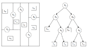
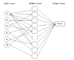
Figure 1: An example of ensemble CT-ANN model with $X_{i}$, where $i=1,2,3,4,5$, as important features obtained using CT, $L_{i}$ be the leaf nodes and OP as CT output.

3 Statistical Properties of the Proposed Model

Our proposed ensemble classifier has the following nomenclature: first, it extracts important features from the feature space using CT algorithm, then it builds one hidden layered ANN model with the important features extracted using CT along with CT outputs as an additional feature. We investigate the statistical properties of the proposed ensemble CT-ANN model by introducing a set of regularity conditions for consistency of CT followed by the importance of CT outputs for further model building. And finally we will discuss the consistency results of ANN algorithm with optimal value of number of neurons in the hidden layer of the model.

Let $\underline{X}$ be the space of all possible values of $p$ features and $C$ be the set of all possible binary outcomes. We are given a training sample with $n$ observations $L=\{(X_{1},C_{1}),(X_{2},C_{2}),...,(X_{n},C_{n})\}$, where $X_{i}=(X_{i1},X_{i2},...,X_{ip})\in\underline{X}$ and $C_{i}\in C$. Also let $\Omega=\{\omega_{1},\omega_{2},...,\omega_{k}\}$ be a partition of the feature space $\underline{X}$. We denote $\widetilde{\Omega}$ as one such partition of $\Omega$. Define $L_{\omega_{i}}=\{(X_{i},C_{i})\in L:X_{i}\in\omega_{i},C_{i}\in C\}$ as the subset of $L$ induced by $\omega_{i}$ and let $L_{\widetilde{\Omega}}$ denote the partition of $L$ induced by $\widetilde{\Omega}$. The information gain (to be introduced later) from the feature space is used to partition $\underline{X}$ into a set $\widetilde{\Omega}$ of nodes and then we can construct a classification function on $\widetilde{\Omega}$. There exists a partitioning classification function $d:\widetilde{\Omega}\rightarrow C$ such that $d$ is constant on every node of $\widetilde{\Omega}$. Now, let us define $\widehat{L}$ to be the space of all learning samples and $\mathbb{D}$ be the space of all partitioning classification function, then $\Phi:\widehat{L}\rightarrow\mathbb{D}$ such that $\Phi(L)=(\psi\circ\phi)(L)$, where $\phi$ maps $L$ to some induced partition $(L)_{\widetilde{\Omega}}$ and $\psi$ is an assigning rule which maps $(L)_{\widetilde{\Omega}}$ to $d$ on the partition $\widetilde{\Omega}$. The most basic reasonable assigning rule $\psi$ is the plurality rule $\psi_{pl}(L_{\widetilde{\Omega}})=d$ such that if $x\in\omega_{i}$, then

$$d(\underline{x})=\arg\max_{c\in C}|L_{c,\omega_{i}}|$$

The plurality rule is used to classify each new point in $\omega_{i}$ as belonging to the class (either 0 or 1 in this case) most common in $L_{\omega_{i}}$. This rule is very important in proving risk consistency of the CT algorithm. Now, let us define a binary split function $s(\omega_{i})$, that maps one node to a pair of nodes, i.e., $s(\omega_{i})=(s_{1}(\omega_{i}),s_{2}(\omega_{i}))=(\omega_{1},\omega_{2})$, then $\omega_{1}\cup\omega_{2}=\omega_{i}$, $\omega_{1}\cap\omega_{2}=\phi$ and $\omega_{1},\omega_{2}\neq\phi$. Binary split function partitions a parent node $\omega_{i}\subseteq\underline{X}$ into a non-empty child nodes $\omega_{1}$ and $\omega_{2}$, called left child and right child node respectively. A set of all potential rules that we will use to split $\underline{X}$ is a finite set $S=\{s_{1},s_{2},....s_{m}\}$.
Define $\mathscr{G}$ as a goodness of split criterion which maps $(\omega_{i},s)$ for all $\omega_{i}\in\underline{X}$ and $s\in S$ to a real number. For any parent node $\omega_{i}$, the goodness of split criterion ranks the split functions. We have used the following impurity function is used as goodness of split criterion:

$$\mathscr{G}(L_{\omega_{i}},s)=H(L_{\omega_{i}})-\frac{|L_{s_{1}(\omega_{i})}|}{|L_{\omega_{i}}|}H(L_{\omega_{1}(t)})-\frac{|L_{s_{2}(\omega_{i})}|}{|L_{\omega_{i}}|}H(L_{\omega_{2}(t)})$$

where, $H$ is taken as Gini Index and can be written as follows:

$$H_{gini}(\omega_{i})=\sum_{c\neq c^{\prime}}\frac{|L_{\omega_{i},c}|}{|L_{\omega_{i}}|}.\frac{|L_{\omega_{i},c^{\prime}}|}{|L_{\omega_{i}}|}$$

This criterion assesses the quality of a split $s(\omega_{i})$ by subtracting the average impurity of the child nodes $\omega_{1},\omega_{2}$ from the impurity of the parent node $\omega_{i}$. The stopping rule in CT is decided based on the minimum number of split in the posterior sample called minsplit ($r(\omega_{i})$). If $r(\omega_{i})$ $\geq\alpha$, then $\omega_{i}$ will split into two child nodes and if $r(\omega_{i})$ $<\alpha$, then $\omega_{i}$ is a leaf node and no more split is required. Here $\alpha$ is determined by the user, though for practice it is usually taken as 10% of the training sample size.

A binary tree-based classification and partitioning scheme $\Phi$ is defined as an assignment rule applied to the limit of a sequence of induced partitions $\phi^{(i)}(L)$, where $\phi^{(i)}(L)$ is the partition of the training sample $L$ induced by the partition $(\phi_{i}\circ\phi_{i-1}\circ....\circ\phi_{1})(\underline{X})$. For every node $\omega_{i}$ in a partition $\widetilde{\Omega}$ such that $r(\omega_{i})$ $\geq\alpha$, then the function $\phi(\widetilde{\Omega})$ splits each node into two child nodes using the binary split in the question set as determined by $\mathscr{G}$. For other nodes $\omega_{i}\in\widetilde{\Omega}$ such that $r(\omega_{i})$ $<\alpha$, then $\phi(\widetilde{\Omega})$ leaves $\omega_{i}$ unchanged. Mathematically,

$$\Phi(L)=(\psi\circ\lim_{i\rightarrow\infty}\phi^{(i)})(L)$$ (1)

where, $\phi^{(i)}(L)=L_{(\phi_{i}\circ\phi_{i-1}\circ....\circ\phi_{1})(\underline{X})}$.

CT as an axis-parallel split on $\mathbb{R}^{p}$ splits a node by dividing into child nodes consisting of either side of some hyperplane. We need to show that CT scheme are well defined, which will be possible only if there exists some induced partition $L^{{}^{\prime}}$ such that $\lim_{i\rightarrow\infty}\phi^{(i)}(L)=L^{{}^{\prime}}$. In fact we need to show that the following lemma holds:

Lemma 1.

If L is a training sample and $\phi^{(i)}$ is defined as above, then there exists $N\in\mathbb{N}\quad\mbox{such that for}\quad n\geq N$

$$\phi^{(n)}(L)=\lim_{i\rightarrow\infty}\phi^{(i)}(L)$$ (2)

Proof.

Let $\{L_{\widetilde{\Omega}}\}$ denote the sequence $\{L,\phi^{1}(L),\phi^{2}(L),...\}$. Defining $\omega_{i}^{max}=\max{\{\omega_{i}\in\widetilde{\Omega}_{i}:r(\omega_{i})>\alpha\}}$ as the size of the largest non-leaf node(s) in $\widetilde{\Omega}_{i}$. Suppose there exists $N\in\mathbb{N}$ such that $(\omega_{i})_{N}^{max}$ does not exist. Then every node in $\widetilde{\Omega}_{N}$ is leaf. For all $n>N$, $\widetilde{\Omega}_{n}=\widetilde{\Omega}_{N}$, then $(2)$ holds. The sequence $\{|\omega_{i}^{max}|\}$ is strictly decreasing if it exists. Further if $\omega_{i+1}^{max}$ exists then $|\omega_{i+1}^{max}|\leq|\omega_{i}^{max}|-1$ and $|\omega_{i}^{max}|\geq 1$ and $|\omega_{1}^{max}|=|L|$. This means that $(\omega_{i})_{|L|}^{max}$ can not exist, so $(2)$ always holds with $N\leq|L|$. ∎

For a wide range of partitioning schemes, the consistency of histogram classification schemes based on data-dependent partitions was shown in the literature [8]. To introduce the theorem, we need to define the following:

For any random variable X and set A, let $\eta_{n,X}(A)=\frac{1}{n}\sum_{i=1}^{n}I(X_{i}\in A)$ be the empirical probability that $X\in A$ based on $n$ observations and $I(z)$ denotes the indicator of an event C. Now let $\mathcal{T}=(\widetilde{\Omega}_{1},\widetilde{\Omega}_{2},...)$ be a finite collection of partitions of a measurement space $\underline{X}$. Define maximal node count of $\mathcal{T}$ as the maximum number of nodes in any partition $\widetilde{\Omega}$ in $\mathcal{T}$ which can be written as $\lambda(\mathcal{T})=\sup_{\widetilde{\Omega}\in\mathcal{T}}|\widetilde{\Omega}|$. Also let, $\Delta(\mathcal{T},L)=|\{L_{\widetilde{\Omega}}:\widetilde{\Omega}\in\mathcal{T}|$ be the number of distinct partitions of a training sample of size $n$ induced by partitions in $\mathcal{T}$. Let $\Delta_{n}(\mathcal{T})$ be the growth function of $\mathcal{T}$ defined as $\Delta_{n}(\mathcal{T})=\sup_{\{L:|L|=n\}}\Delta(\mathcal{T},L)$. Growth function of $\mathcal{T}$ is the maximum number of distinct partitions $L_{\widetilde{\Omega}}$ which partition $\widetilde{\Omega}$ in $\mathcal{T}$ can induce in any training sample with $n$ observations. Take any class $\mathscr{A}\subseteq\mathbb{R}^{p}$, $S_{n}(\mathscr{A})=\max_{\{B\subset\mathbb{R}^{p}:|B|=n\}}|A\cap B:A\in\mathscr{A}|$ is the maximum number of partitions of $B$ induced by $\mathscr{A}$, where $B$ is some $n$ point subset of $\mathbb{R}^{p}$, called shatter coefficient. For a partition $\widetilde{\Omega}$ of $X$, let $\widetilde{\Omega}[x\in X]=\{\omega\in\widetilde{\Omega}:x\in\omega\}$ be the node $\omega$ in $\widetilde{\Omega}$ which contains $x$. For a set $A\subseteq\mathbb{R}^{p}$, let $D(A)=\sup_{x,y\in A}\parallel x-y\parallel$ be the diameter of $A$. Now, for the sake of completeness we are rewriting the Theorem 2 of [8] in our context:

Theorem 1.

Let $(\underline{X},\underline{Y})$ be a random vector taking values in $\mathbb{R}^{p}\times C$ and $L$ be the set of first n outcomes of $(\underline{X},\underline{Y})$. Suppose that $\Phi$ is a partition and classification scheme such that $\Phi(L)=(\psi_{pl}\circ\phi)(L)$, where $\psi_{pl}$ is the plurality rule and $\phi(L)=(L)_{\tilde{\Omega_{n}}}$ for some $\tilde{\Omega}_{n}\in\mathcal{T}_{n}$, where

$$\mathcal{T}_{n}=\{\phi(\ell_{n}):P(L=\ell_{n})>0\}.$$

Also suppose that all the binary split functions in the question set associated with $\Phi$ are hyperplane splits. As $n\rightarrow\infty$, if the following regularity conditions hold:

$$\frac{\lambda(\mathcal{T}_{n})}{n}\rightarrow 0$$ (3)

$$\frac{log(\triangle_{n}(\mathcal{T}_{n}))}{n}\rightarrow 0$$ (4)

and for every $\gamma>0$ and $\delta\in(0,1)$,

$$\inf_{S\subseteq\mathbb{R}^{p}:\eta_{x}(S)\geq 1-\delta}\eta_{x}({x:diam(\tilde{\Omega}_{n}[x]\cap S)>\gamma})\rightarrow 0$$ (5)

with probability 1. then $\Phi$ is risk consistent.

Proof.

For the proof of Theorem 1, one may refer to [8]. ∎

Remark.

Now instead of considering histogram-based partitioning and classification schemes, we are going to show the risk consistency of CT as defined above. We can produce a simultaneous result with conditions (3) and (4) of Theorem 1 replaced by a simple condition. Though the shrinking cell condition ((5) of Theorem 1) is also assumed.

Theorem 2.

Suppose $(\underline{X},\underline{Y})$ be a random vector in $\mathbb{R}^{p}\times\ C$ and $L$ be the training set consisting of $n$ outcomes of $(\underline{X},\underline{Y})$. Let $\Phi$ be a classification tree scheme such that

$$\Phi(L)=(\psi_{pl}\circ\lim_{i\to\infty}\phi^{(i)})(L)$$

where, $\psi_{pl}$ is the plurality rule and $\phi(L)=(L)_{\tilde{\Omega}_{n}}$ for some $\tilde{\Omega}_{n}\in\mathcal{T}_{n}$, where

$$\mathcal{T}_{n}=\{\lim_{i\to\infty}\phi^{(i)}(\ell_{n}):P(L=\ell_{n})>0\}.$$

Suppose that all the split function in CT in the question set associated with $\Phi$ are axis-parallel splits. Finally if for every n and $w_{i}\in\tilde{\Omega}_{n}$, the induced subset $L_{w_{i}}$ has cardinality $\geq k_{n}$, where $\frac{k_{n}}{log(n))}\rightarrow\infty$ and (5) holds true, then $\Phi$ is risk consistent.

Proof.

Since $|w_{i}|\geq k_{n}\quad\forall\quad w_{i}\in\tilde{\Omega}_{n}$, we can write

$$|\tilde{\Omega}_{n}|\leq\frac{n}{k_{n}}$$ (6)

for every $\tilde{\Omega}_{n}\in\mathcal{T}_{n}$ and in that case, we will have $\frac{\lambda(\mathcal{T}_{n})}{n}\leq\frac{1}{k_{n}}$.
As $n\rightarrow\infty$, we can see $\frac{1}{k_{n}}\rightarrow 0$ which gives $\frac{\lambda(\mathcal{T}_{n})}{n}\rightarrow 0$. Hence condition (3) holds true.

Now for every $\tilde{\Omega}_{n}\in\mathcal{T}_{n}$, using Cover’s theorem [17], any binary split of $\mathbb{R}^{p}$ can divide $n$ points in $\mathbb{R}^{p}$ in at most $n^{p}$ ways. Using equation (6), we can write

$$\Delta_{n}(\mathcal{T}_{n})\leq(n^{p})^{\frac{n}{k_{n}}}$$

and consequently

$$\frac{log(\Delta_{n}(\mathcal{T}_{n}))}{n}\leq p\frac{log(n)}{k_{n}}$$ (7)

As $n\rightarrow\infty$, RHS of equation (7) goes to 0. So condition (4) of Theorem 1 also holds and hence the theorem. ∎

Remark.

Note that no assumptions are made on the distribution of the pair $(\underline{X},\underline{Y})\in\mathbb{R}^{p}\times C$. Also sub-linear growth of the number of cells (condition (3)) and sub-exponential growth of a combinatorial complexity measure (condition (4)) are not required, instead a more flexible restriction such as if each cell of $L_{\omega_{i}}$ has cardinality $\geq k_{n}$ and $\frac{k_{n}}{log(n))}\rightarrow\infty$, then CT is said to be risk consistent. So, feature selection using CT algorithm is justified and now we are going to check the importance of CT output in further model building. It is also noted that the choice of important features based on CT is a greedy algorithm and the optimality of local choices of the best feature for a node doesn’t guarantee that the constructed tree will be globally optimal [18].

Using CT given features, a list of important features are selected from $p$ available features. It is noted that CT output also plays an important role in further modeling. To see the importance of CT given classification results (to be denoted by $OP$ in rest of the paper) as a relevant feature, we introduce a non-linear measure of correlation between any feature and the actual class levels, namely C-correlation [19], as follows:

Definition: C-correlation is the correlation between any feature $F_{i}$ and the actual class levels C, denoted by $SU_{F_{i},C}$. Symmetrical uncertainty (SU) [20] is defined as follows:

$$SU(X,Y)=2\bigg{[}\frac{H(X)-H(X|Y)}{H(X)+H(Y)}\bigg{]}$$ (8)

where, $H(X)$ is the entropy of a variable $X$ and $H(X|Y)$ is the entropy of $X$ while $Y$ is observed. We can heuristically decide a feature to be highly correlated with class $C$ if $SU_{F_{i},C}>\beta$, where $\beta$ is a relevant threshold to be determined by users. Using definition we can conclude that $OP$ can be taken as a non-redundant feature for further model building. This also improves the performance of the model at a significant rate, to be shown in Section 4.

Now, we build ANN model with CT given features and $OP$ as another input feature in ANN model. The dimension of input layer in ANN model, denoted by $d_{m}(\leq{p})$, is the number of important features obtained by CT + 1. We will use one hidden layer in ANN model due to the incorporation of $OP$ as an input information in the model. It should be noted that one-hidden layer neural networks yield strong universal consistency and there is little theoretical gain in considering two or more hidden layered neural networks [11]. In ensemble CT-ANN model, we have used one hidden layer with $k$ neurons. This makes the proposed ensemble binary classifier less complex and less time consuming while implementing the model. Our next objective is to state the sufficient condition for universal consistency and then finding out the optimal value of $k$. Before stating the sufficient conditions for the consistency of the algorithm and optimal number of nodes in hidden layer for practical use of the model, let us define the followings:

Definition: A sigmoid function $\sigma(x)$ is called a logistic squasher if it is non-decreasing, $\lim_{x\rightarrow\infty}\sigma(x)=0$ and $\lim_{x\rightarrow-\infty}\sigma(x)=1$ with $\sigma(x)=\frac{1}{1+exp{(-x)}}$.

Given $n$ training sequence $\xi_{n}=\{(Z_{1},Y_{1}),...,(Z_{n},Y_{n})\}$ of $n$ i.i.d copies of $(\underline{Z},\underline{Y})$ taking values from $\mathbb{R}^{d_{m}}\times C$, a classification rule realized by a one-hidden layered neural network is chosen to minimize the empirical $L_{1}$ risk. Define the $L_{1}$ error of a function $\psi:\mathbb{R}^{d_{m}}\rightarrow\{0,1\}$ by $J(\psi)=E\{|\psi(Z)-Y|\}$.

Consider a neural network with one hidden layer with bounded output weight having $k$ hidden neurons and let $\sigma$ be a logistic squasher. Let $\mathscr{F}_{n,k}$ be the class of neural networks with logistic squasher defined as

$$\mathscr{F}_{n,k}=\Bigg{\{}\sum_{i=1}^{k}c_{i}\sigma(a_{i}^{T}z+b_{i})+c_{0}:k\in\mathbb{N},a_{i}\in\mathbb{R}^{d_{m}},b_{i},c_{i}\in\mathbb{R},\sum_{i=0}^{k}|c_{i}|\leq\beta_{n}\Bigg{\}}$$

Let $\psi_{n}$ be the function that minimizes the empirical $L_{1}$ error over $\psi_{n}\in\mathscr{F}_{n,k}$. Lugosi and Zeger (1995) has shown that if $k$ and $\beta_{n}$ satisfy

$$k\rightarrow\infty,\quad\beta_{n}\rightarrow\infty,\quad\frac{k\beta_{n}^{4}log(k\beta_{n}^{2})}{n}\rightarrow 0$$

and there exists $\delta(>0)$ such that $\frac{\beta_{n}^{4}}{n^{1-\delta}}\rightarrow 0$, then the classification rule

$$g_{n}(z)=\begin{cases}0,&\text{if $\psi_{n}(z)\leq 1/2$}.\\ 1,&\text{otherwise}.\end{cases}$$ (9)

is strongly universally consistent [10].

Alternatively, $J(\psi_{n})-J^{*}\rightarrow 0$ in probability, where $J(\psi_{n})=E\{|\psi_{n}(Z)-Y||\xi_{n}\}$ and $J^{*}=\inf_{\psi_{n}}J(\psi_{n})$ [11]. Write

$$J(\psi_{n})-J^{*}=\bigg{(}J(\psi_{n})-\inf_{\psi\in\mathscr{F}_{n,k}}J(\psi)\bigg{)}+\bigg{(}\inf_{\psi\in\mathscr{F}_{n,k}}J(\psi)-J^{*}\bigg{)}$$

where, $(J(\psi_{n})-\inf_{\psi\in\mathscr{F}_{n,k}}J(\psi))$ is called estimation error and $(\inf_{\psi\in\mathscr{F}_{n,k}}J(\psi)-J^{*})$ is called approximation error.

Now, we are going to find out the optimal choice of $k$ using the regularity conditions of strong universal convergence and the idea of obtaining upper bounds on the rate of convergence, i.e., how fast $J(\psi_{n})$ approaches to zero [21]. To obtain an upper bound on the rate of convergence, we will have to impose some regularity conditions on the posteriori probabilities. Though in case of rate of convergence of estimation error, we will have a distribution-free upper bound [9]. And to obtain the optimal value of $k$, it is enough to find upper bounds of the estimation and approximation errors. The upper bound of approximation error investigated by Baron [22], is given in Lemma 2.

Lemma 2.

Assume that there is a compact set $E\subset\mathbb{R}^{d_{m}}$ such that $Pr\{Z\in E\}=1$ and the Fourier transform $\widetilde{P_{0}}(w)$ of $P_{0}(z)$ satisfies

$$\int_{\mathbb{R}^{d_{m}}}|\omega||\widetilde{P_{0}}(\omega)|d\omega<\infty$$

then

$$\inf_{\psi\in\mathscr{F}_{n,k}}E\bigg{(}f(Z,\psi)-P_{0}(Z)\bigg{)}^{2}\leq\frac{c}{k},$$

where c is a constant depending on the distribution.

Remark.

The previous condition on Fourier transformation and extensive discussion on the properties of functions satisfying the condition (including logistic squasher function) are given in the paper of Baron [22].

Proposition 1.

For a fixed $d_{m}$, let $\psi_{n}\in\mathscr{F}_{c}$. The neural network satisfying regularity conditions of strong universal consistency and if the conditions of Lemma 2 holds, then the optimal choice of $k$ is $O\bigg{(}\sqrt{\frac{n}{d_{m}log(n)}}\bigg{)}$.

Proof.

Applying Cauchy-Schwarz inequality in lemma 2, we can write

$$\inf_{\psi\in\mathscr{F}_{n,k}}E\bigg{|}f(Z,\psi)-P_{0}(Z)\bigg{|}=O\bigg{(}\frac{1}{\sqrt{k}}\bigg{)}$$

It is well known [23] that for any $\psi$

$$J(\psi)-J^{*}\leq 2E\bigg{|}f(Z,\psi)-P_{0}(Z)\bigg{|}$$

So, the upper bound of approximation error is found to be $O\bigg{(}\frac{1}{\sqrt{k}}\bigg{)}$.
Though the approximation error goes to zero as the number of neurons goes to infinity for strongly universally consistent classifier. But in practical implementation number of neurons is often fixed (eg., can’t be increased with the size of the training sample grows). Now, it is enough to bound the estimation error.

Let us define $r(\psi_{n})=E(J(\psi_{n}))=P(\psi_{n}(Z)\neq Y)$ is the average error probability of $\psi_{n}$. Using lemma 3 of [9], we can write that the estimation error is always $O\bigg{(}\sqrt{\frac{kd_{m}log(n)}{n}}\bigg{)}$.
Bringing the above facts together, we can write

$$r(\psi_{n})-J^{*}=O\bigg{(}\sqrt{\frac{kd_{m}log(n)}{n}}+\frac{1}{\sqrt{k}}\bigg{)}$$

Now, to find optimal value of $k$, the problem reduces to equating $\sqrt{\frac{kd_{m}log(n)}{n}}$ with $\frac{1}{\sqrt{k}}$, which gives $k=O\bigg{(}\sqrt{\frac{n}{d_{m}log(n)}}\bigg{)}$. ∎

Remark.

We can see a remarkable property of ensemble CT-ANN model from Proposition 1. Since for this class of posteriori probability function as shown in Lemma 2, the rate of convergence does not necessarily depend on the dimension, in the sense that the exponent is constant. Thus, it can be concluded that the proposed model will not suffer from the curse of dimensionality.

The optimal value of hidden nodes is found to be $O\bigg{(}\sqrt{\frac{n}{d_{m}log(n)}}\bigg{)}$ in the ensemble CT-ANN model. For practical use, if the data set is small, the recommendation is to use $\bigg{(}\sqrt{\frac{n}{d_{m}log(n)}}\bigg{)}$ for achieving utmost accuracy of the proposed model. Since the proposed ensemble classifier possesses the desirable statistical properties, the classifier can be called robust. The practical usefulness and competitiveness of the proposed classifier in solving real life feature selection cum classification problems will be shown in Section 4.

4 Experimental Evaluation

4.1 The datasets

The proposed model is evaluated using six publicly available medical data sets from Kaggle and UCI Machine Learning repository dealing with various diseases like breast cancer, pima diabetes, heart disease, promoter gene sequences, SPECT heart images, etc. These binary classification data sets have limited number of observations and high-dimensional feature spaces. Breast cancer data set has 9 discrete features where as pima diabetes data set consists of 8 continuous features in the input space [24]. Heart disease data set originally contained a total of 303 examples for 13 continuous features, out of which 6 contained missing class values and 27 are disputed examples which were removed from the data set. Promoter gene sequences data set has 57 sequential DNA nucleotides attributes. SPECT images data set is represented by 22 binary features that have either 0 or 1 values, but the data set is imbalanced in nature. Wisconsin breast cancer data set consists of 699 examples carrying 9 continuous features in the input space [25]. Table 1 gives a summary about these data sets.

Table 1: Characteristics of the data sets used in experimental evaluation

Dataset	Classes	Objects	Number of	Number of	Number of
		$(n)$	feature $(p)$	$(+)$ve instances	$(-)$ve instances
breast cancer	2	286	9	85	201
heart disease	2	270	13	120	150
pima diabetes	2	768	8	500	268
promoter gene sequences	2	106	57	53	53
SPECT heart images	2	267	22	55	212
wisconsin breast cancer	2	699	9	458	241

4.2 Performance measures

The performance evaluation measures used in our experimental analysis are based on the confusion matrix. Higher the value of performance metrics, the better the classifier is. The expressions for different performance measures as follows:
Classification Accuracy = $\frac{(TP+TN)}{(TP+TN+FP+FN)}$; F-measure =$2\frac{\big{(}\mbox{Precision}\times\mbox{Recall}\big{)}}{\big{(}\mbox{Precision}+\mbox{Recall}\big{)}}$;
where, Precision = $\frac{TP}{TP+FP}$; Recall = $\frac{TP}{TP+FN}$; and
TP (True Positive): correct positive prediction; FP (False Positive): incorrect positive prediction; TN (True Negative): correct negative prediction; FN (False Negative): incorrect negative prediction.

4.3 Analysis of Results

In order to show the impact of the proposed 2-step pipeline model, it is applied to the high-dimensional small or medium sized medical data sets. These are such types of data sets in which not only classification is the task but also feature selection plays a vital role before it. We shuffled the observations in each of the 6 medical data sets randomly and split it into training, validation and test data sets in a ration of 50 : 25 : 25. We have also repeated each of the experiments 10 times with different randomly assigned training, validation and testing data sets.

Our proposed algorithm is compared with Classification Tree (CT), Random Forest (RF), Support Vector Machine (SVM), Artificial Neural Network (ANN) with 1HL and 2HL, Entropy Nets, Tsai Neural Tree (NT) [5], Deep Neural Decision Trees (DNDT) [7] based on the different performance metrics. All these classifiers are implemented in R Statistical software on a PC with 2.1GHz processor with 8GB memory other than DNDT. We compared the proposed model with 1-HL ANN and 2-HL ANN without employing feature selection. Since the data sets are small and medium sized, going beyond 2HL ANN will over-fit the data set [11] and this is also reminiscent of universal approximation theorem [2]. For 1HL ANN, number of hidden neurons used is $k\thickapprox\sqrt{n}$ [11] and for 2HL ANN, 2/3 of the input sizes are taken as the number of neurons in the 1st HL and 1/3 of the input sizes in case of 2nd HL [26]. In a similar way Tsai Neural Tree (NT) were also built and the accuracy levels were compared. DNDT searches tree structure and parameter with stochastic gradient descent which was implemented in TensorFlow [27], and it is a kind of GPU-accelerated computing [7]. Breiman’s random forest [28] also has an in-built feature selection mechanism which was implemented using party implementation in R and results are reported in Table 2.

To apply our proposed model to the medical data sets, we first apply CT with minsplit (as defined in Section 3) as 10% of the training sample size using the rpart package implementation in R. CT model uses gini index of diversity with the available input feature space. The variable importance indicator $C_{p}$ was used for selection of variables to enter or leave CT model. Based on the results of CT, important variables or features were chosen in the final model along with CT output. The number of reduced features after feature selection using CT are reported in Table 2. The number of hidden neurons in the hidden layer is calculated using this formula $k=\sqrt{\frac{n}{d_{m}log(n)}}$, where $n$ is the number of training samples and $d_{m}$ as the number of input features in neural networks. We have further normalized the data sets before training the neural network. Min-max method is used for scaling the data in an interval of $[0,1]$. For small or medium data sets, our model recommends using the upper bound of the number of neurons in the HL of the ensemble model. The ensemble CT-ANN model is trained using neuralnet implementation in R. Training time and memory requirement for our proposed model is quite low as compared with DNDT which needs availability of GPU. Table 2 gives the obtained results from different classifiers used for experimental evaluation over 6 medical data sets. We can conclude from Table 2 that the proposed model achieves overall highest accuracy while working with reduced features as compared to other state-of-the-arts for most of the data sets and remains competitive for other few data sets as well.

Table 2: Results (and their standard deviation) of classification algorithms over 6 medical data sets

Classifiers	Data set	The number of (reduced)	Classification	F-measure
		features after	accuracy
		feature selection	(%)
CT	breast cancer	7	68.26 (6.40)	0.70 (0.07)
	heart disease	7	76.50 (4.50)	0.81 (0.03)
	pima diabetes	6	71.85 (4.94)	0.74 (0.03)
	promoter gene sequences	17	69.43 (2.78)	0.73 (0.01)
	SPECT heart images	9	75.70 (1.56)	0.78 (0.00)
	wisconsin breast cancer	8	94.20 (2.98)	0.89 (0.01)
RF	breast cancer	6	69.00 (7.30)	0.72 (0.07)
	heart disease	8	80.19 (4.23)	0.84 (0.01)
	pima diabetes	6	73.49 (4.12)	0.76 (0.03)
	promoter gene sequences	20	71.26 (1.97)	0.75 (0.03)
	SPECT heart images	10	79.70 (1.23)	0.82 (0.01)
	wisconsin breast cancer	8	95.75 (2.01)	0.96 (0.02)
SVM	breast cancer	9	64.62 (5.21)	0.68 (0.05)
	heart disease	13	78.95 (4.89)	0.83 (0.01)
	pima diabetes	8	70.39 (3.56)	0.72 (0.03)
	promoter gene sequences	57	59.35 (1.37)	0.63 (0.02)
	SPECT heart images	22	83.46 (1.29)	0.85 (0.00)
	wisconsin breast cancer	9	93.30 (2.78)	0.94 (0.01)
ANN (with 1HL)	breast cancer	9	61.58 (5.89)	0.64 (0.04)
	heart disease	13	73.56 (5.44)	0.79 (0.02)
	pima diabetes	8	66.78 (4.58)	0.69 (0.04)
	promoter gene sequences	57	61.77 (3.46)	0.65 (0.02)
	SPECT heart images	22	79.69 (0.23)	0.81 (0.01)
	wisconsin breast cancer	9	94.80 (2.01)	0.96 (0.01)
ANN (with 2HL)	breast cancer	9	62.20 (5.12)	0.64 (0.03)
	heart disease	13	78.81 (3.96)	0.82 (0.03)
	pima diabetes	8	69.78 (3.89)	0.73 (0.02)
	promoter gene sequences	57	63.46 (2.19)	0.68 (0.02)
	SPECT heart images	22	82.71 (0.78)	0.84 (0.01)
	wisconsin breast cancer	9	95.60 (2.54)	0.96 (0.10)
Entropy Nets	breast cancer	7	69.00 (6.25)	0.72 (0.05)
	heart disease	7	79.59 (4.78)	0.83 (0.01)
	pima diabetes	6	69.50 (4.05)	0.72 (0.02)
	promoter gene sequences	17	66.23 (1.98)	0.70 (0.01)
	SPECT heart images	9	76.64 (1.70)	0.78 (0.01)
	wisconsin breast cancer	8	95.96 (2.18)	0.96 (0.00)
TSai NT	breast cancer	7	69.45 (7.17)	0.71 (0.07)
	heart disease	7	80.25 (4.68)	0.85 (0.01)
	pima diabetes	6	71.59 (4.19)	0.74 (0.03)
	promoter gene sequences	17	70.67 (2.83)	0.74 (0.02)
	SPECT heart images	9	76.95 (1.27)	0.78 (0.01)
	wisconsin breast cancer	8	97.40 (2.11)	0.98 (0.01)
DNDT	breast cancer	8	66.12 (7.81)	0.68 (0.08)
	heart disease	7	81.05 (3.89)	0.86 (0.02)
	pima diabetes	6	69.21 (5.08)	0.72 (0.05)
	promoter gene sequences	17	69.06 (1.75)	0.71 (0.01)
	SPECT heart images	10	75.50 (0.89)	0.77 (0.00)
	wisconsin breast cancer	7	94.25 (2.14)	0.95 (0.00)
Proposed Model	breast cancer	7	72.80 (6.54)	0.77 (0.06)
	heart disease	7	82.78 (4.78)	0.89 (0.02)
	pima diabetes	6	76.10 (4.45)	0.79 (0.04)
	promoter gene sequences	17	75.40 (1.50)	0.79 (0.01)
	SPECT heart images	9	81.03 (0.56)	0.82 (0.00)
	wisconsin breast cancer	8	97.30 (1.05)	0.98 (0.00)

5 Conclusion and Discussions

In this paper, a novel nonparametric ensemble classifier is proposed to achieve higher accuracy in classification performance with very little computational cost (by working with a subset of input features). Our proposed feature selection cum classification model is robust in nature. Ensemble CT-ANN model is shown to be universally consistent and less time consuming during the actual implementation. We have also found the optimal value of the number of neurons in the hidden layer so that the user will have less tuning parameters to be controlled. The proposed model when applied to real life data sets performed better compared to other state-of-the-art models for most of the data sets and remained competitive for the few other data sets. Situations when feature selection is not a job in classification problems, our model may not be too effective. But the ensemble classifier will have an edge where the data analysis requires important variable selections in the early stage followed by predictions using classifiers for limited data sets. In the light of current advances in ANN, one might ask a simple question : What is the need of a two-step pipeline (like ensemble CT-ANN model) over advanced ANN models ?

A straight-cut answer to this question could be unwise. The primary goal of ’statistics’ is to make scientific inferences from the model compared to building a “black-box-like” model which may perform well for some specific data sets, but may not be considered as a general theory [29]. Our proposed model is robust, universally consistent, easily interpretable and highly useful for high dimensional small or medium sized data sets (for example, medical data sets) to perform feature selection cum classification task. Advanced ANN models (say, deep neural net) are highly complex, over-parameterized models and found useful when the data sets are very large (like image, audio and video data sets) [29]. Nevertheless, no model can have dominant advantage and one may also refer to no free lunch theorems [30]. Normally, for every new finding there will always be a trade-off between accuracy, interpretability and complexity of the model [30]. There are many future scope of research of this paper. One scope is to extend the model for multi-class classification problems. Another interesting area for research is to improve the ensemble model especially for imbalanced data sets.

References

- [1] L. Breiman, Classification and regression trees, Routledge, 2017.
- [2] K. Hornik, M. Stinchcombe, H. White, Multilayer feedforward networks are universal approximators, Neural networks 2 (5) (1989) 359–366.
- [3] I. K. Sethi, Entropy nets: from decision trees to neural networks, Proceedings of the IEEE 78 (10) (1990) 1605–1613.
- [4] A. Sakar, R. J. Mammone, Growing and pruning neural tree networks, IEEE Transactions on Computers 42 (3) (1993) 291–299.
- [5] C.-C. Tsai, M.-C. Lu, C.-C. Wei, Decision tree-based classifier combined with neural-based predictor for water-stage forecasts in a river basin during typhoons: a case study in taiwan, Environmental engineering science 29 (2) (2012) 108–116.
- [6] J. Sirat, J. Nadal, Neural trees: a new tool for classification, Network: Computation in Neural Systems 1 (4) (1990) 423–438.
- [7] Y. Yang, I. G. Morillo, T. M. Hospedales, Deep neural decision trees, arXiv preprint arXiv:1806.06988.
- [8] G. Lugosi, A. Nobel, Consistency of data-driven histogram methods for density estimation and classification, The Annals of Statistics 24 (2) (1996) 687–706.
- [9] A. Faragó, G. Lugosi, Strong universal consistency of neural network classifiers, IEEE Transactions on Information Theory 39 (4) (1993) 1146–1151.
- [10] G. Lugosi, K. Zeger, Nonparametric estimation via empirical risk minimization, IEEE Transactions on information theory 41 (3) (1995) 677–687.
- [11] L. Devroye, L. Györfi, G. Lugosi, A probabilistic theory of pattern recognition, Vol. 31, Springer Science & Business Media, 2013.
- [12] R. Balestriero, Neural decision trees, arXiv preprint arXiv:1702.07360.
- [13] G. Biau, E. Scornet, J. Welbl, Neural random forests, Sankhya A (2016) 1–40.
- [14] T. Chakraborty, S. Chattopadhyay, A. K. Chakraborty, A novel hybridization of classification trees and artificial neural networks for selection of students in a business school, OPSEARCH 55 (2) (2018) 434–446.
- [15] J. R. Quinlan, C4. 5: Programming for machine learning, Morgan Kauffmann 38 (1993) 48.
- [16] T. Chakraborty, A. K. Chakraborty, S. Chattopadhyay, A novel distribution-free hybrid regression model for manufacturing process efficiency improvement, arXiv preprint arXiv:1804.08698.
- [17] T. M. Cover, Geometrical and statistical properties of systems of linear inequalities with applications in pattern recognition, IEEE transactions on electronic computers (3) (1965) 326–334.
- [18] L. I. Kuncheva, Combining pattern classifiers: methods and algorithms, John Wiley & Sons, 2004.
- [19] L. Yu, H. Liu, Efficient feature selection via analysis of relevance and redundancy, Journal of machine learning research 5 (Oct) (2004) 1205–1224.
- [20] W. H. Press, S. A. Teukolsky, W. T. Vetterling, B. P. Flannery, Numerical recipes in c: the art of scientific computing, Cambridge University Press, Cambridge, MA, 131 (1992) 243–262.
- [21] L. Györfi, M. Kohler, A. Krzyzak, H. Walk, A distribution-free theory of nonparametric regression, Springer Science & Business Media, 2006.
- [22] A. R. Barron, Universal approximation bounds for superpositions of a sigmoidal function, IEEE Transactions on Information theory 39 (3) (1993) 930–945.
- [23] L. Devroye, L. Gyorfi, Nonparametric density estimation: The l1 view, New York : John Wiley & Sons, 1985.
- [24] J. J. Rodriguez, L. I. Kuncheva, C. J. Alonso, Rotation forest: A new classifier ensemble method, IEEE transactions on pattern analysis and machine intelligence 28 (10) (2006) 1619–1630.
- [25] L. A. Kurgan, K. J. Cios, R. Tadeusiewicz, M. Ogiela, L. S. Goodenday, Knowledge discovery approach to automated cardiac spect diagnosis, Artificial intelligence in medicine 23 (2) (2001) 149–169.
- [26] Z.-H. Zhou, J. Wu, W. Tang, Ensembling neural networks: many could be better than all, Artificial intelligence 137 (1-2) (2002) 239–263.
- [27] M. Abadi, P. Barham, J. Chen, Z. Chen, A. Davis, J. Dean, M. Devin, S. Ghemawat, G. Irving, M. Isard, et al., Tensorflow: a system for large-scale machine learning., in: OSDI, Vol. 16, 2016, pp. 265–283.
- [28] L. Breiman, Random forests, Machine learning 45 (1) (2001) 5–32.
- [29] D. B. Dunson, Statistics in the big data era: Failures of the machine, Statistics & Probability Letters 136 (2018) 4–9.
- [30] D. H. Wolpert, The lack of a priori distinctions between learning algorithms, Neural computation 8 (7) (1996) 1341–1390.