Numerical Approximation of Incompressible Navier-Stokes Equations Based on an Auxiliary Energy Variable

Abstract

We present a numerical scheme for approximating the incompressible Navier-Stokes equations based on an auxiliary variable associated with the total system energy. By introducing a dynamic equation for the auxiliary variable and reformulating the Navier-Stokes equations into an equivalent system, the scheme satisfies a discrete energy stability property in terms of a modified energy and it allows for an efficient solution algorithm and implementation. Within each time step, the algorithm involves the computations of two pressure fields and two velocity fields by solving several de-coupled individual linear algebraic systems with constant coefficient matrices, together with the solution of a nonlinear algebraic equation about a scalar number involving a negligible cost. A number of numerical experiments are presented to demonstrate the accuracy and the performance of the presented algorithm.

Keywords: energy stability; unconditional stability; Navier-Stokes equations; incompressible flows; auxiliary variable

1 Introduction

We focus on the numerical approximation of the incompressible Navier-Stokes equations, which form the basis for simulations of single-phase incompressible flows and turbulence KravchenkoM2000 ; MaKK2000 ; DongKER2006 ; Dong2007 . The momentum equations for two-phase and multiphase flow problems YueFLS2004 ; AbelsGG2012 ; DongS2012 ; Dong2018 often take a form analogous to the incompressible Navier-Stokes equations with a similar mathematical structure. Developing efficient and effective algorithms for incompressible Navier-Stokes equations therefore can have implications in fields far beyond incompressible flows.

An essential tradeoff confronting a practitioner of computational fluid dynamics (CFD) is between the desire to be able to use larger time step sizes (permitted by accuracy/stability) and the computational cost. On one end of the spectrum, unconditionally energy-stable schemes (see e.g. Shen1992 ; SimoA1994 ; LabovskyLMNR2009 ; DongS2010 ; Sanderse2013 ; JiangMRT2016 ; ChenSZ2018 , among others) can alleviate the time step size constraint, and one can concentrate on the accuracy requirement when choosing a time step size in a simulation task. This however comes with a downside. Within each time step energy-stable schemes typically involve the solution of a system of nonlinear algebraic equations or a system of linear algebraic equations with a variable and time-dependent coefficient matrix, inducing a high computation cost due to the Newton nonlinear iterations and the need for frequent re-computations of the coefficient matrices. This can render the overall approach inefficient, and therefore such schemes are not often used in large-scale production simulations in practice, especially for dynamic problems. On the other end of the spectrum, semi-implicit splitting type (or fractional-step) schemes (see e.g. Chorin1968 ; Temam1969 ; KimM1985 ; KarniadakisIO1991 ; BrownCM2001 ; XuP2001 ; GuermondS2003 ; LiuLP2007 ; HyoungsuK2011 ; SersonMS2016 , the review article GuermondMS2006 , and the references therein) de-couple the computations for the velocity and the pressure fields, and all the coefficient matrices are constant and can be pre-computed. Such schemes have a low computational cost. But they are only conditionally stable, and the time step size that can be used is restricted by e.g. CFL type conditions. Thanks to their low cost, semi-implicit schemes are very popular in large-scale production simulations for flow physics investigations (see e.g. MaKK2000 ; DongKER2006 ; Dong2009 ; DongZ2011 ).

We present in this work a numerical scheme for the incompressible Navier-Stokes equations that in a sense resides somewhere between the two extremes on the spectrum of methods. The salient feature of this scheme is the introduction of an auxiliary variable (which is a scalar number) associated with the total energy of the Navier-Stokes system. This idea is inspired by a recent work ShenXY2018 for gradient-type dynamical systems. The incompressible Navier-Stokes equations are then reformulated into an equivalent system employing the auxiliary energy variable, and a numerical scheme is devised to approximate the reformulated system. Within a time step, the algorithm requires the computations of two pressure fields and two velocity fields, as well as the solution of a nonlinear algebraic equation about a scalar number. The computation for each of the pressure/velocity fields involves a linear algebraic system with a constant coefficient matrix that can be pre-computed. Solving the nonlinear algebraic equation requires Newton iterations, but its cost is negligible (accounting for $1\sim 2\%$ of the total cost per time step) because this nonlinear equation is about a scalar number, not a field function. This scheme can be shown to satisfy a discrete energy stability property in terms of a modified energy. Numerical experiments show that the algorithm allows the use of very large time step sizes for steady flow problems, and for unsteady flow problems it appears to be not as effective in terms of the time step size. The amount of operations (and the computational cost) of this algorithm per time step is approximately twice that of the semi-implicit scheme from Dong2015clesobc , which is only conditionally stable.

The novelties of this work lie in several aspects: (i) the introduction of the auxiliary energy variable into and the resultant reformulation of the Navier-Stokes system; (ii) the numerical scheme for approximating the reformulated system of equations; and (iii) the efficient solution procedure for overcoming the difficulty caused by the unknown auxiliary variable in the implementation of the scheme.

The rest of this paper is structured as follows. In Section 2 we introduce an auxiliary energy variable and reformulate the Navier-Stokes equations based on this variable. A numerical scheme is presented for approximating the reformulated equivalent system. We then discuss how to implement the scheme, and in particular how to overcome the challenge caused by the unknown auxiliary variable in the implementation. In Section 3 we present several representative numerical simulations to test the accuracy and performance of the algorithm. Section 4 concludes the presentation with some closing remarks.

2 Auxiliary Variable-Based Algorithm for Incompressible Navier-Stokes Equations

2.1 Reformulated Equations and Numerical Scheme Formulation

Consider an incompressible flow contained in some domain $\Omega$ in two or three dimensions, whose boundary is denoted by $\partial\Omega$. The dynamics of the flow is described by the incompressible Navier-Stokes equations, given in a non-dimensional form as follows,

$$\frac{\partial\mathbf{u}}{\partial t}+\mathbf{N}(\mathbf{u})+\nabla p-\nu\nabla^{2}\mathbf{u}=\mathbf{f},$$ (1a)

$$\nabla\cdot\mathbf{u}=0,$$ (1b)

where $\mathbf{x}$ and $t$ denote the spatial coordinate and time, $\mathbf{u}(\mathbf{x},t)$ and $p(\mathbf{x},t)$ are respectively the normalized velocity and pressure, $\mathbf{f}(\mathbf{x},t)$ is an external body force, and $\mathbf{N}(\mathbf{u})$ is the convection term, $\mathbf{N}(\mathbf{u})=\mathbf{u}\cdot\nabla\mathbf{u}$. $\nu$ denotes the inverse of the Reynolds number $Re$,

$$\nu=\frac{1}{Re}=\frac{\nu_{f}}{U_{0}L}$$ (2)

where $U_{0}$ is the characteristic velocity scale, $L$ is the characteristic length scale, and $\nu_{f}$ is the kinematic viscosity of the fluid. On the domain boundary $\partial\Omega$ we assume that the velocity is known

$$\mathbf{u}=\mathbf{w}(\mathbf{x},t),\quad\text{on}\ \partial\Omega$$ (3)

where $\mathbf{w}$ denotes the boundary velocity. The system is supplemented by the initial condition

$$\mathbf{u}(\mathbf{x},0)=\mathbf{u}_{in}(\mathbf{x})$$ (4)

where the initial velocity distribution $\mathbf{u}_{in}$ is assumed to be compatible with the boundary condition (3) on $\partial\Omega$ and satisfies the equation (1b). In the governing equations (1a)–(1b), only the pressure gradient $\nabla p$ is physically meaningful, and the absolute pressure value is not fixed (pressure can be shifted by an arbitrary constant). In order to fix the pressure values in the numerical solution we impose the following often-used condition

$$\int_{\Omega}p=0.$$ (5)

Consider a shifted total energy of the system

$$E(t)=E[\mathbf{u}]=C_{0}+\int_{\Omega}\frac{1}{2}|\mathbf{u}|^{2}$$ (6)

where $C_{0}$ is a chosen constant such that $E(t)>0$ for all $t\geqslant 0$. Define an auxiliary variable $R(t)$ by

$$R(t)=\sqrt{E(t)}.$$ (7)

Then

$$2R\frac{dR}{dt}=\frac{dE}{dt}=\int_{\Omega}\frac{\partial\mathbf{u}}{\partial t}\cdot\mathbf{u}=\int_{\Omega}\left(\frac{\partial\mathbf{u}}{\partial t}+\mathbf{u}\cdot\nabla\mathbf{u}\right)\cdot\mathbf{u}-\int_{\partial\Omega}(\mathbf{n}\cdot\mathbf{u})\frac{1}{2}|\mathbf{u}|^{2}$$ (8)

where $\mathbf{n}$ is the outward-pointing unit vector normal to the boundary $\partial\Omega$, and we have used integration by part, the equation (1b), and the divergence theorem. It should be emphasized that both $R(t)$ and $E(t)$ are scalar variables, not field functions. At $t=0$,

$$R(0)=\left(C_{0}+\int_{\Omega}\frac{1}{2}|\mathbf{u}_{in}|^{2}\right)^{\frac{1}{2}}.$$ (9)

In light of the definition (7), we re-write equation (1a) into an equivalent form

$$\frac{\partial\mathbf{u}}{\partial t}+\frac{R(t)}{\sqrt{E(t)}}\mathbf{N}(\mathbf{u})+\nabla p-\nu\nabla^{2}\mathbf{u}=\mathbf{f}.$$ (10)

We also re-write equation (8) into an equivalent form

$$2R\frac{dR}{dt}=\int_{\Omega}\left[\frac{\partial\mathbf{u}}{\partial t}+\frac{R(t)}{\sqrt{E(t)}}\mathbf{N}(\mathbf{u})\right]\cdot\mathbf{u}-\int_{\partial\Omega}(\mathbf{n}\cdot\mathbf{u})\frac{1}{2}|\mathbf{u}|^{2}.$$ (11)

The original system consisting of the equations (1a)–(1b), (3) and (4) is equivalent to the reformulated system consisting of equations (10), (1b), (11), together with the boundary condition (3) and the initial conditions (4) and (9), in which $E(t)$ is given by (6). We next focus on this reformulated equivalent system of equations, and present a numerical scheme for approximating this system.

Let $n\geqslant 0$ denote the time step index, and $(\cdot)^{n}$ denote the variable $(\cdot)$ at time step $n$. Let $J$ ($J=1$ or $2$) denote the temporal order of accuracy of the scheme. We set

$$\mathbf{u}^{0}=u_{in}(\mathbf{x}),\quad R^{0}=\sqrt{E(0)}=\sqrt{C_{0}+\int_{\Omega}\frac{1}{2}|\mathbf{u}^{0}|^{2}}.$$ (12)

Then given ($\mathbf{u}^{n}$, $p^{n}$, $R^{n}$), we compute ($\mathbf{u}^{n+1}$, $p^{n+1}$, $R^{n+1}$) through the following scheme

$$\frac{\gamma_{0}\mathbf{u}^{n+1}-\hat{\mathbf{u}}}{\Delta t}+\frac{R^{n+1}}{\sqrt{E^{n+1}}}\mathbf{N}(\bar{\mathbf{u}}^{n+1})+\nabla p^{n+1}-\nu\nabla^{2}\mathbf{u}^{n+1}=\mathbf{f}^{n+1},$$ (13a)

$$\nabla\cdot\mathbf{u}^{n+1}=0,$$ (13b)

$$\begin{split}2R^{n+1}\frac{\gamma_{0}R^{n+1}-\hat{R}}{\Delta t}=&\int_{\Omega}\left[\frac{\gamma_{0}\mathbf{u}^{n+1}-\hat{\mathbf{u}}}{\Delta t}+\frac{R^{n+1}}{\sqrt{E^{n+1}}}\mathbf{N}(\bar{\mathbf{u}}^{n+1})\right]\cdot\mathbf{u}^{n+1}-\int_{\partial\Omega}(\mathbf{n}\cdot\mathbf{u}^{n+1})\frac{1}{2}|\mathbf{u}^{n+1}|^{2},\end{split}$$ (13c)

$$\mathbf{u}^{n+1}=\mathbf{w}^{n+1},\quad\text{on}\ \partial\Omega.$$ (13d)

$$E^{n+1}=\int_{\Omega}\frac{1}{2}\left|\mathbf{u}^{n+1}\right|^{2}+C_{0}.$$ (13e)

$$\int_{\Omega}p^{n+1}=0.$$ (13f)

$\Delta t$ is the time step size in the above equations. If $\chi$ denotes a generic variable, then in the above equations $\frac{1}{\Delta t}(\gamma_{0}\chi^{n+1}-\hat{\chi})$ is the approximation of $\left.\frac{\partial\chi}{\partial t}\right|^{n+1}$ based on the $J$-th order backward differentiation formula (BDF), with $\gamma_{0}$ and $\hat{\chi}$ defined specifically by

$$\hat{\chi}=\left\{\begin{array}[]{ll}\chi^{n},&J=1,\\ 2\chi^{n}-\frac{1}{2}\chi^{n-1},&J=2;\end{array}\right.\qquad\gamma_{0}=\left\{\begin{array}[]{ll}1,&J=1,\\ 3/2,&J=2.\end{array}\right.$$ (14)

$\bar{\mathbf{u}}^{n+1}$ denotes a $J$-th order explicit approximation of $\mathbf{u}^{n+1}$, given by

$$\bar{\mathbf{u}}^{n+1}=\left\{\begin{array}[]{ll}\mathbf{u}^{n},&J=1,\\ 2\mathbf{u}^{n}-\mathbf{u}^{n-1},&J=2.\end{array}\right.$$ (15)

Taking the $L^{2}$ inner product between $\mathbf{u}^{n+1}$ and equation (13a) leads to

$$\int_{\Omega}\left[\frac{\gamma_{0}\mathbf{u}^{n+1}-\hat{\mathbf{u}}}{\Delta t}+\frac{R^{n+1}}{\sqrt{E^{n+1}}}\mathbf{N}(\bar{\mathbf{u}}^{n+1})\right]\cdot\mathbf{u}^{n+1}+\int_{\partial\Omega}(\mathbf{n}\cdot\mathbf{u}^{n+1})p^{n+1}\\ -\nu\int_{\partial\Omega}(\mathbf{n}\cdot\nabla\mathbf{u}^{n+1})\cdot\mathbf{u}^{n+1}+\nu\int_{\Omega}\|\nabla\mathbf{u}^{n+1}\|^{2}=\int_{\Omega}\mathbf{f}^{n+1}\cdot\mathbf{u}^{n+1}$$ (16)

where we have used integration by part, the divergence theorem, and the equation (13b). Sum up equations (13c) and (16), and we have

$$2R^{n+1}\frac{\gamma_{0}R^{n+1}-\hat{R}}{\Delta t}=-\nu\int_{\Omega}\|\nabla\mathbf{u}^{n+1}\|^{2}+\int_{\Omega}\mathbf{f}^{n+1}\cdot\mathbf{u}^{n+1}\\ +\int_{\partial\Omega}\left(-p^{n+1}\mathbf{n}+\nu\mathbf{n}\cdot\nabla\mathbf{u}^{n+1}-\frac{1}{2}|\mathbf{w}^{n+1}|^{2}\mathbf{n}\right)\cdot\mathbf{w}^{n+1}$$ (17)

where we have used equation (13d). Note the following relations

$$2R^{n+1}(\gamma_{0}R^{n+1}-\hat{R})=2R^{n+1}(R^{n+1}-R^{n})=|R^{n+1}|^{2}-|R^{n}|^{2}+|R^{n+1}-R^{n}|^{2},\quad\text{if}\ J=1;$$ (18a)

$$\begin{split}2R^{n+1}(\gamma_{0}R^{n+1}-\hat{R})=&2R^{n+1}\left(\frac{3}{2}R^{n+1}-2R^{n}+\frac{1}{2}R^{n}\right)\\ =&\frac{1}{2}\left(|R^{n+1}|^{2}-|R^{n}|^{2}\right)+\frac{1}{2}\left(\left|2R^{n+1}-R^{n}\right|^{2}-\left|2R^{n}-R^{n-1}\right|^{2}\right)\\ &+\frac{1}{2}\left|R^{n+1}-2R^{n}+R^{n-1}\right|^{2},\quad\text{if}\ J=2.\end{split}$$ (18b)

Combining the above equations, we obtain the following stability result about the scheme:

Theorem 2.1.

In the absence of the external force $\mathbf{f}$ and with zero boundary velocity $\mathbf{w}$, the scheme represented by equations (13a)–(13f) satisfies the following property:

$$Q^{n+1}-Q^{n}=-\left|D^{n+1}\right|^{2}-\nu\Delta t\int_{\Omega}\|\nabla\mathbf{u}^{n+1}\|^{2}$$ (19)

where

$$Q^{n}=\left\{\begin{array}[]{ll}|R^{n}|^{2},&J=1,\\ \frac{1}{2}\left(|R^{n}|^{2}+|2R^{n}-R^{n-1}|^{2}\right),&J=2;\end{array}\right.\ \ D^{n+1}=\left\{\begin{array}[]{ll}R^{n+1}-R^{n},&J=1,\\ \frac{1}{\sqrt{2}}\left(R^{n+1}-2R^{n}+R^{n-1}\right),&J=2.\end{array}\right.$$ (20)

2.2 Solution Algorithm and Implementation

We next consider how to implement the algorithm represented by the equations (13a)–(13f). Even though $R^{n+1}$ and $E^{n+1}$ are both implicit and $E^{n+1}$ involves the integral of the unknown field function $\mathbf{u}^{n+1}$ over the domain, the scheme can be implemented in an efficient way, thanks to the fact that $R^{n+1}$ and $E^{n+1}$ are scalar numbers, not field functions. We employ $C^{0}$ spectral elements SherwinK1995 ; KarniadakisS2005 ; ZhengD2011 ; ChenSX2012 for spatial discretizations in the current work.

Let

$$S=\frac{R^{n+1}}{\sqrt{E^{n+1}}},\quad E(S)=E^{n+1}=\int_{\Omega}\frac{1}{2}|\mathbf{u}^{n+1}|^{2}+C_{0}.$$ (21)

Then equation (13a) can be written as

$$\frac{\gamma_{0}}{\Delta t}\mathbf{u}^{n+1}+\nabla p^{n+1}-\nu\nabla^{2}\mathbf{u}^{n+1}=\mathbf{G}^{n+1}-S\mathbf{N}(\bar{\mathbf{u}}^{n+1})$$ (22)

where $\mathbf{G}^{n+1}=\mathbf{f}^{n+1}+\frac{\hat{\mathbf{u}}}{\Delta t}$. In light of (13b), equation (22) can be transformed into

$$\frac{\gamma_{0}}{\Delta t}\mathbf{u}^{n+1}+\nabla p^{n+1}=\mathbf{G}^{n+1}-S\mathbf{N}(\bar{\mathbf{u}}^{n+1})-\nu\nabla\times\nabla\times\mathbf{u}^{n+1}.$$ (23)

We would like to derive the weak forms for the pressure and velocity in the spatially continuous space first. The discrete function spaces for these variables will be specified later. Let $q(\mathbf{x})$ denote an arbitrary test function in the continuous space. Taking the $L^{2}$ inner product between $\nabla q$ and equation (23), we get

$$\int_{\Omega}\nabla p^{n+1}\cdot\nabla q=\int_{\Omega}\left[\mathbf{G}^{n+1}-S\mathbf{N}(\bar{\mathbf{u}}^{n+1})\right]\cdot\nabla q-\nu\int_{\partial\Omega}\mathbf{n}\times\bm{\omega}^{n+1}\cdot\nabla q-\frac{\gamma_{0}}{\Delta t}\int_{\partial\Omega}\mathbf{n}\cdot\mathbf{w}^{n+1}q,\quad\forall q,$$ (24)

where $\bm{\omega}=\nabla\times\mathbf{u}$ is the vorticity, and we have used the integration by part, the divergence theorem, equations (13b) and (13d), and the identity $\int_{\Omega}\nabla\times\bm{\omega}\cdot\nabla q=\int_{\partial\Omega}\mathbf{n}\times\bm{\omega}\cdot\nabla q.$ Equation (24) couples the pressure and the velocity because of the vorticity $\bm{\omega}^{n+1}$ (tangent component) on the boundary. In order to simplify the implementation, we will make the the following approximation, $\left.\mathbf{n}\times\bm{\omega}^{n+1}\right|_{\partial\Omega}\approx\left.\mathbf{n}\times\bar{\bm{\omega}}^{n+1}\right|_{\partial\Omega}$, where $\bar{\bm{\omega}}^{n+1}=\nabla\times\bar{\mathbf{u}}^{n+1}$ is the vorticity based on the explicitly approximated velocity defined in (15). This only slightly reduces the robustness in terms of stability, but significantly simplifies the implementation and reduces the computations. Employing this approximation, we transform (24) into

$$\int_{\Omega}\nabla p^{n+1}\cdot\nabla q=\int_{\Omega}\left[\mathbf{G}^{n+1}-S\mathbf{N}(\bar{\mathbf{u}}^{n+1})\right]\cdot\nabla q-\nu\int_{\partial\Omega}\mathbf{n}\times\bar{\bm{\omega}}^{n+1}\cdot\nabla q-\frac{\gamma_{0}}{\Delta t}\int_{\partial\Omega}\mathbf{n}\cdot\mathbf{w}^{n+1}q,\quad\forall q.$$ (25)

This equation, together with equation (13f), can be solved for $p^{n+1}$, provided that the unknown scalar value $S=\frac{R^{n+1}}{\sqrt{E^{n+1}}}$ is given.

Exploiting the fact that $S$ is a scalar number (not a field function), we solve equations (25) and (13f) for $p^{n+1}$ as follows. Define two field variables $p_{1}^{n+1}$ and $p_{2}^{n+1}$ as solutions to the following two problems:
For $p_{1}^{n+1}$:

$$\int_{\Omega}\nabla p_{1}^{n+1}\cdot\nabla q=\int_{\Omega}\mathbf{G}^{n+1}\cdot\nabla q-\nu\int_{\partial\Omega}\mathbf{n}\times\bar{\bm{\omega}}^{n+1}\cdot\nabla q-\frac{\gamma_{0}}{\Delta t}\int_{\partial\Omega}\mathbf{n}\cdot\mathbf{w}^{n+1}q,\quad\forall q.$$ (26a)

$$\int_{\Omega}p_{1}^{n+1}=0.$$ (26b)

For $p_{2}^{n+1}$:

$$\int_{\Omega}\nabla p_{2}^{n+1}\cdot\nabla q=-\int_{\Omega}\mathbf{N}(\bar{\mathbf{u}}^{n+1})\cdot\nabla q,\quad\forall q.$$ (27a)

$$\int_{\Omega}p_{2}^{n+1}=0.$$ (27b)

Then it is straightforward to verify that the solution to equations (25) and (13f) is given by

$$p^{n+1}=p_{1}^{n+1}+Sp_{2}^{n+1}$$ (28)

where $S$ is to be determined later.

In light of (28), we re-write equation (22) as

$$\frac{\gamma_{0}}{\nu\Delta t}\mathbf{u}^{n+1}-\nabla^{2}\mathbf{u}^{n+1}=\frac{1}{\nu}(\mathbf{G}^{n+1}-\nabla p_{1}^{n+1})-\frac{S}{\nu}\left[\mathbf{N}(\bar{\mathbf{u}}^{n+1})+\nabla p_{2}^{n+1}\right].$$ (29)

Let $\varphi(\mathbf{x})$ denote an arbitrary test function that vanishes on $\partial\Omega$, i.e. $\left.\varphi\right|_{\partial\Omega}=0$. Taking the $L^{2}$ inner product between $\varphi$ and the equation (29), we obtain the weak form about $\mathbf{u}^{n+1}$,

$$\frac{\gamma_{0}}{\nu\Delta t}\int_{\Omega}\mathbf{u}^{n+1}\varphi+\int_{\Omega}\nabla\varphi\cdot\nabla\mathbf{u}^{n+1}=\frac{1}{\nu}\int_{\Omega}(\mathbf{G}^{n+1}-\nabla p_{1}^{n+1})\varphi\\ -\frac{S}{\nu}\int_{\Omega}\left[\mathbf{N}(\bar{\mathbf{u}}^{n+1})+\nabla p_{2}^{n+1}\right]\varphi,\quad\forall\varphi\ \text{with}\ \varphi|_{\partial\Omega}=0,$$ (30)

where we have used integration by part, the divergence theorem, and the fact that $\left.\varphi\right|_{\partial\Omega}=0$. This equation, together with equation (13d), can be solved for $\mathbf{u}^{n+1}$, provided that $S$ is known.

We again exploit the fact that $S$ is a scalar number, and solve these equations for $\mathbf{u}^{n+1}$ as follows. Define two field variables $\mathbf{u}_{1}^{n+1}$ and $\mathbf{u}_{2}^{n+1}$ as solutions to the following two problems:
For $\mathbf{u}_{1}^{n+1}$:

$$\frac{\gamma_{0}}{\nu\Delta t}\int_{\Omega}\mathbf{u}_{1}^{n+1}\varphi+\int_{\Omega}\nabla\varphi\cdot\nabla\mathbf{u}_{1}^{n+1}=\frac{1}{\nu}\int_{\Omega}(\mathbf{G}^{n+1}-\nabla p_{1}^{n+1})\varphi,\quad\forall\varphi\ \text{with}\ \varphi|_{\partial\Omega}=0.$$ (31a)

$$\mathbf{u}_{1}^{n+1}=\mathbf{w}^{n+1},\quad\text{on}\ \partial\Omega.$$ (31b)

For $\mathbf{u}_{2}^{n+1}$:

$$\frac{\gamma_{0}}{\nu\Delta t}\int_{\Omega}\mathbf{u}_{2}^{n+1}\varphi+\int_{\Omega}\nabla\varphi\cdot\nabla\mathbf{u}_{2}^{n+1}=-\frac{1}{\nu}\int_{\Omega}\left[\mathbf{N}(\bar{\mathbf{u}}^{n+1})+\nabla p_{2}^{n+1}\right]\varphi,\quad\forall\varphi\ \text{with}\ \varphi|_{\partial\Omega}=0.$$ (32a)

$$\mathbf{u}_{2}^{n+1}=0,\quad\text{on}\ \partial\Omega.$$ (32b)

Then the solution $\mathbf{u}^{n+1}$ to equations (30) and (13d) is given by

$$\mathbf{u}^{n+1}=\mathbf{u}_{1}^{n+1}+S\mathbf{u}_{2}^{n+1},$$ (33)

where $S$ is to be determined.

We re-write equation (13c) into

$$\frac{2}{\Delta t}R^{n+1}(\gamma_{0}R^{n+1}-\hat{R})\frac{R^{n+1}}{\sqrt{E^{n+1}}}-\frac{\gamma_{0}}{\Delta t}\frac{R^{n+1}}{\sqrt{E^{n+1}}}\int_{\Omega}|\mathbf{u}^{n+1}|^{2}+\frac{1}{\Delta t}\frac{R^{n+1}}{\sqrt{E^{n+1}}}\int_{\Omega}\hat{\mathbf{u}}\cdot\mathbf{u}^{n+1}\\ -\left(\frac{R^{n+1}}{\sqrt{E^{n+1}}}\right)^{2}\int_{\Omega}\mathbf{N}(\bar{\mathbf{u}}^{n+1})\cdot\mathbf{u}^{n+1}+\frac{R^{n+1}}{\sqrt{E^{n+1}}}\int_{\partial\Omega}(\mathbf{n}\cdot\mathbf{u}^{n+1})\frac{1}{2}|\mathbf{u}^{n+1}|^{2}=0,$$ (34)

where we have multiplied both sides of equation (13c) by $\frac{R^{n+1}}{\sqrt{E^{n+1}}}$. We observe that this can improve the robustness of the scheme when the time step size $\Delta t$ becomes large. This is a scalar nonlinear equation, and it will be solved for $S$.

In light of equation (33), we have

$$E^{n+1}=E(S)=C_{0}+\int_{\Omega}\frac{1}{2}|\mathbf{u}^{n+1}|^{2}=A_{0}+A_{1}S+A_{2}S^{2},$$ (35)

where

$$\begin{split}A_{0}=C_{0}+\int_{\Omega}\frac{1}{2}|\mathbf{u}_{1}^{n+1}|^{2},\quad A_{1}=\int_{\Omega}\mathbf{u}_{1}^{n+1}\cdot\mathbf{u}_{2}^{n+1},\quad A_{2}=\int_{\Omega}\frac{1}{2}|\mathbf{u}_{2}^{n+1}|^{2}.\end{split}$$ (36)

In light of equations (21), (13d), (28) and (33), we can transform equation (34) into

$$F(S)=\frac{2\gamma_{0}}{\Delta t}S(S^{2}-1)E(S)-\frac{2\hat{R}}{\Delta t}S^{2}\sqrt{E(S)}+B_{0}S+B_{1}S^{2}+B_{2}S^{3}=0$$ (37)

where $\hat{R}$ is defined by (14) and

$$\left\{\begin{split}&B_{0}=\frac{2\gamma_{0}}{\Delta t}C_{0}+\frac{1}{\Delta t}\int_{\Omega}\hat{\mathbf{u}}\cdot\mathbf{u}_{1}^{n+1}+\int_{\partial\Omega}(\mathbf{n}\cdot\mathbf{w}^{n+1})\frac{1}{2}|\mathbf{w}^{n+1}|^{2},\\ &B_{1}=\frac{1}{\Delta t}\int_{\Omega}\hat{\mathbf{u}}\cdot\mathbf{u}_{2}^{n+1}-\int_{\Omega}\mathbf{N}(\bar{\mathbf{u}}^{n+1})\cdot\mathbf{u}_{1}^{n+1},\\ &B_{2}=-\int_{\Omega}\mathbf{N}(\bar{\mathbf{u}}^{n+1})\cdot\mathbf{u}_{2}^{n+1}.\end{split}\right.$$ (38)

Equation (37) is a nonlinear scalar equation about $S$. It can be solved for $S$ using the Newton’s method with an initial guess $S=1$. The cost of this computation is very small and is essentially negligible compared to the total cost within a time step, which will be shown by the numerical experiments in Section 3. With $S$ known, $E^{n+1}$ can be computed based on equation (35), and $R^{n+1}$ can be computed using equation (21). The velocity $\mathbf{u}^{n+1}$ and pressure $p^{n+1}$ are then given by equations (33) and (28).

Let us now consider the spatial discretization of the equations (26a)–(27b) and (31a)–(32b). We discretize the domain $\Omega$ with a mesh consisting of $N_{el}$ conforming spectral elements. Let the positive integer $K$ denote the element order, which represents a measure of the highest polynomial degree in the polynomial expansions of the field variables within an element. Let $\Omega_{h}$ denote the discretized domain, $\partial\Omega_{h}$ denote the boundary of $\Omega_{h}$, and $\Omega_{h}^{e}$ ($1\leqslant e\leqslant N_{el}$) denote the element $e$. Define two function spaces

$$\left\{\begin{split}&X=\{\ v\in H^{1}(\Omega_{h})\ :\ v\ \text{is a polynomial characterized by}\ K\ \text{on}\ \Omega_{h}^{e},\ \text{for}\ 1\leqslant e\leqslant N_{el}\ \},\\ &X_{0}=\{\ v\in X\ :\ \left.v\right|_{\partial\Omega_{h}}=0\ \}.\end{split}\right.$$ (39)

In the following let $d$ ($d=2$ or $3$) denote the spatial dimension, and the subscript in $(\cdot)_{h}$ denote the discretized version of the variable $(\cdot)$. The fully discretized equations corresponding to (26a)–(27b) are:
For $p_{1h}^{n+1}$:   find $p_{1h}^{n+1}\in X$ such that

$$\int_{\Omega_{h}}\nabla p_{1h}^{n+1}\cdot\nabla q_{h}=\int_{\Omega_{h}}\mathbf{G}_{h}^{n+1}\cdot\nabla q_{h}-\nu\int_{\partial\Omega_{h}}\mathbf{n}_{h}\times\bar{\bm{\omega}}_{h}^{n+1}\cdot\nabla q_{h}-\frac{\gamma_{0}}{\Delta t}\int_{\partial\Omega_{h}}\mathbf{n}_{h}\cdot\mathbf{w}_{h}^{n+1}q_{h},\ \forall q_{h}\in X.$$ (40a)

$$\int_{\Omega_{h}}p_{1h}^{n+1}=0.$$ (40b)

For $p_{2h}^{n+1}$:   find $p_{2h}^{n+1}\in X$ such that

$$\int_{\Omega_{h}}\nabla p_{2h}^{n+1}\cdot\nabla q_{h}=-\int_{\Omega_{h}}\mathbf{N}(\bar{\mathbf{u}}_{h}^{n+1})\cdot\nabla q_{h},\quad\forall q_{h}\in X.$$ (41a)

$$\int_{\Omega_{h}}p_{2h}^{n+1}=0.$$ (41b)

The fully discretized equations corresponding to (31a)–(32b) are:
For $\mathbf{u}_{1h}^{n+1}$:   find $\mathbf{u}_{1h}^{n+1}\in[X]^{d}$ such that

$$\frac{\gamma_{0}}{\nu\Delta t}\int_{\Omega_{h}}\mathbf{u}_{1h}^{n+1}\varphi_{h}+\int_{\Omega_{h}}\nabla\varphi_{h}\cdot\nabla\mathbf{u}_{1h}^{n+1}=\frac{1}{\nu}\int_{\Omega_{h}}\left(\mathbf{G}_{h}^{n+1}-\nabla p_{1h}^{n+1}\right)\varphi_{h},\quad\forall\varphi_{h}\in X_{0}.$$ (42a)

$$\mathbf{u}_{1h}^{n+1}=\mathbf{w}_{h}^{n+1},\quad\text{on}\ \partial\Omega_{h}.$$ (42b)

For $\mathbf{u}_{2h}^{n+1}$:   find $\mathbf{u}_{2h}^{n+1}\in[X]^{d}$ such that

$$\frac{\gamma_{0}}{\nu\Delta t}\int_{\Omega_{h}}\mathbf{u}_{2h}^{n+1}\varphi_{h}+\int_{\Omega_{h}}\nabla\varphi_{h}\cdot\nabla\mathbf{u}_{2h}^{n+1}=-\frac{1}{\nu}\int_{\Omega_{h}}\left[\mathbf{N}(\bar{\mathbf{u}}_{h}^{n+1})+\nabla p_{2h}^{n+1}\right]\varphi_{h},\quad\forall\varphi_{h}\in X_{0}.$$ (43a)

$$\mathbf{u}_{2h}^{n+1}=0,\quad\text{on}\ \partial\Omega_{h}.$$ (43b)

Combining the above discussions, we arrive at the final solution algorithm. It involves the following steps:

1. Solve equations (40a)–(40b) for $p_{1}^{n+1}$;
   Solve equations (42a)–(42b) for $\mathbf{u}_{1}^{n+1}$.

2. Solve equations (41a)–(41b) for $p_{2}^{n+1}$;
   Solve equations (43a)–(43b) for $\mathbf{u}_{2}^{n+1}$.

3. Compute the coefficients $A_{0}$, $A_{1}$ and $A_{2}$ based on (36);
   Compute the coefficients $B_{0}$, $B_{1}$ and $B_{2}$ based on (38).

4. Solve equation (37) for $S$ using the Newton’s method with an initial guess $S=1$.

5. Compute $\mathbf{u}^{n+1}$ from equation (33);
   Compute $p^{n+1}$ from equation (28);
   Compute $E^{n+1}$ from equation (35);
   Compute $R^{n+1}$ by $R^{n+1}=S\sqrt{E^{n+1}}$.

It is noted that the linear algebraic systems for $p_{1}^{n+1}$, $p_{2}^{n+1}$, $\mathbf{u}_{1}^{n+1}$, and $\mathbf{u}_{2}^{n+1}$ all involve constant and time-independent coefficient matrices, which can be pre-computed during pre-processing.

3 Representative Numerical Examples

We next use several numerical examples in two dimensions to test the performance and the accuracy of the algorithm presented in the previous section. The spatial and temporal convergence rates of the scheme will first be demonstrated using a contrived analytic solution to the incompressible Navier-Stokes equations. Then we will employ the method to study a steady-flow problem (Kovasznay flow) and the flow past a circular cylinder in a periodic channel for a range of Reynolds numbers.

3.1 Convergence Rates

In this subsection we employ a manufactured analytic solution to the incompressible Navier-Stokes equations to investigate the spatial and temporal convergence rates of the algorithm developed herein.

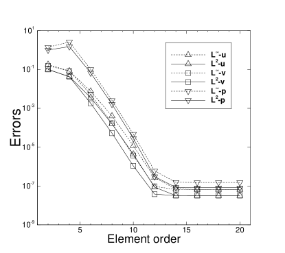
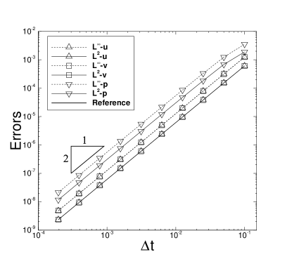
(a) (a)

Figure 1: Convergence tests: (a) Numerical errors vs. element order (fixed $\Delta t=0.001$ and $t_{f}=0.1$). (b) Numerical errors vs. $\Delta t$ (fixed element order $16$ and $t_{f}=0.2$).

Consider a rectangular domain $0\leqslant x\leqslant 2$ and $-1\leqslant y\leqslant 1$, and the following solution to the Navier-Stokes equations (1a)–(1b) and (5) on this domain:

$$\left\{\begin{split}&u=2\cos(\pi y)\sin(\pi x)\sin t,\\ &v=-2\sin(\pi y)\cos(\pi x)\sin t,\\ &p=2\sin(\pi y)\sin(\pi x)\cos t,\end{split}\right.$$ (44)

where $u$ and $v$ are the two components of the velocity $\mathbf{u}$. In equation (1a) the external body force $\mathbf{f}$ is chosen such that the expressions in (44) satisfy this equation.

We simulate this problem using the algorithm from Section 2. The domain is discretized with two uniform elements along the $x$ direction. On the domain boundary we impose the Dirichlet boundary condition (3), in which the boundary velocity $\mathbf{w}$ is chosen based on the analytic expressions in (44). The initial velocity $\mathbf{u}_{in}$ is chosen according to the analytic expressions in (44) by setting $t=0$.

We integrate the Navier-Stokes equations in time from $t=0$ to $t=t_{f}$ ($t_{f}$ to be specified next). Then we compare the numerical solutions of different flow variables at $t=t_{f}$ with the analytic expressions from (44), and the errors in different norms are computed and recorded. The element order and the time step size $\Delta t$ are varied systematically in the simulations in order to study their effects on the numerical errors. We employ a non-dimensional viscosity $\nu=0.01$ for this problem, and the constant $C_{0}$ in equation (6) is fixed at $C_{0}=1.0$ in the simulations.

In the spatial convergence tests, we employ a fixed $t_{f}=0.1$ and $\Delta t=0.001$, and vary the element order systematically between $2$ and $20$. The errors at $t=t_{f}$ between the numerical solution and the analytic solution in $L^{\infty}$ and $L^{2}$ norms have been computed corresponding to all these element orders. Figure 1(a) shows these numerical errors as a function of the element order for this group of tests. For element orders $12$ and below we observe an exponential decrease in the numerical errors as the element order increases. As the element order increases beyond $14$, we observe a saturation in the numerical errors due to the temporal truncation error. The error curves for different flow variables level off approximately at a level around $10^{-7}$. These results are indicative of an exponential convergence rate in space for the current method.

In the temporal convergence tests, we fix the integration time at $t_{f}=0.2$ and the element order at a large value $16$, and then vary the time step size systematically between $\Delta t=0.1$ and $\Delta t=1.953125\times 10^{-4}$. Figure 1(b) shows the $L^{\infty}$ and $L^{2}$ errors of the velocity and pressure as a function of $\Delta t$, plotted in logarithmic scales for both axes. A second-order convergence rate in time is clearly observed with the method developed herein.

3.2 Kovasznay Flow

In this subsection we test the proposed method using a steady-state problem, the Kovasznay flow Kovasznay1948 , for which the exact solution of the flow field is available.

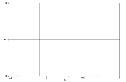
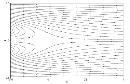
(a) (b)

Figure 2: Kovasznay flow: (a) Flow domain and mesh of $6$ quadrilateral elements; (b) Streamlines.

Specifically, we consider the domain $0\leqslant x\leqslant 1$ and $-0.5\leqslant y\leqslant 0.5$, as depicted in Figure 2(a). The Kovasznay flow solution to the Navier-Stokes equations (1a)–(1b) (with $\mathbf{f}=0$) is given by the following expressions for the velocity $\mathbf{u}=(u,v)$ and pressure:

$$\left\{\begin{split}&u=1-e^{\lambda x}\cos(2\pi y),\\ &v=\frac{\lambda}{2\pi}e^{\lambda x}\sin(2\pi y),\\ &p=\frac{1}{2}(1-e^{2\lambda x}),\end{split}\right.$$ (45)

where the constant $\lambda=\frac{1}{2\nu}-\sqrt{\frac{1}{4\nu^{2}}+4\pi^{2}}.$ The flow pattern for this solution is illustrated by the streamlines shown in Figure 2(b), which is similar to that behind an obstacle. We employ a non-dimensional viscosity $\nu=0.025$ for this problem.

To simulate the problem, we discretize the domain using $6$ quadrilateral elements as shown in Figure 2(a). The element orders and the time step sizes are varied in the tests and will be specified subsequently. In the Navier-Stokes equation (1a) the external body force is set to $\mathbf{f}=0$. On the four boundaries Dirichlet type conditions are imposed for the velocity according to the expression given in (45). We set a zero initial velocity, $\mathbf{u}_{in}=0$, in the initial condition (4). The simulations have been performed for a sufficiently long time until the steady state is reached. Then the errors of the numerical solutions against the exact solution as given by (45) are computed, as well as the norms of the flow variables.

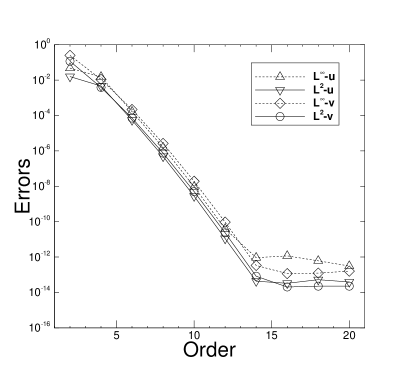
Figure 3: Kovasznay flow: $L^{\infty}$ and $L^{2}$ errors of the steady-state velocity as a function of the element order. Results are obtained with $\Delta t=0.005$ and $C_{0}=0.01$.

Figure 3 shows the $L^{\infty}$ and $L^{2}$ errors of the steady-state velocity from the simulations as a function of the element order. In this group of tests the time step size is fixed at $\Delta t=0.005$, and the constant $C_{0}$ in equation (6) is $C_{0}=0.01$, while the element order has been varied systematically between $2$ and $20$. The errors of the steady-state velocity decrease exponentially with increasing element order, until they saturate at a level about $10^{-13}$ as the element order increases to $14$ and beyond.

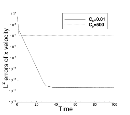
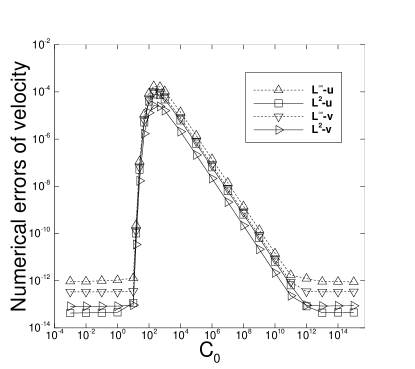
(a) (b)

Figure 4: Effect of $C_{0}$ value on the simulation errors of Kovasznay flow: (a) Time histories of $L^{2}$ errors of the $x$ velocity obtained with $C_{0}=0.01$ and $C_{0}=500$. (b) Numerical errors of the steady-state velocities as a function of $C_{0}$. Results are obtained using $\Delta t=0.005$ and an element order $14$.

We observe that the value for the constant $C_{0}$ in (6) has a marked influence on the accuracy of the solution to the steady-state velocity for this problem. This is demonstrated by the results in Figure 4. Figure 4(a) shows the $L^{2}$ errors of the $x$ velocity component as a function of time as the simulation proceeds. These results are for two constant values, $C_{0}=0.01$ and $C_{0}=500$. The time step size is $\Delta t=0.005$ and the element order is $14$ in these simulations. An initial reduction in the numerical error is evident from both history curves. But after this initial stage the error corresponding to $C_{0}=500$ levels off at a value around $10^{-4}$, while for $C_{0}=0.01$ the error levels off at a value between $10^{-14}$ and $10^{-13}$. In light of this difference in the error levels, we have studied the $C_{0}$ effect more systematically. We vary $C_{0}$ between $0.001$ and $10^{15}$, and for each $C_{0}$ value the errors of the steady-state velocity is computed and recorded. In Figure 4(b) we show the errors of the steady-state velocity as a function of $C_{0}$. Fixed values of $\Delta t=0.005$ and an element order $14$ have been employed in these tests. As $C_{0}$ increases from $10^{-3}$ to about $10$, the numerical errors remain essentially the same (around $10^{-13}$). Then as $C_{0}$ increases from $10$ to about $500$ there is a sharp increase in the numerical errors, and the errors peak at a $C_{0}$ value between $200$ and $500$ (reaching a level of about $10^{-4}$). Beyond $C_{0}=500$, the numerical errors decrease with increasing $C_{0}$, and the errors are approximately inverse proportional to $C_{0}$ between $C_{0}=1000$ and $C_{0}=10^{11}$. As $C_{0}$ increases to $10^{12}$ and beyond, the numerical errors remain essentially the same, at a level around $10^{-13}$. These results suggest that using a small $C_{0}$ or a very large $C_{0}$ in the algorithm seems more favorable in terms of the accuracy. We employ a constant value $C_{0}=0.01$ for all the results reported subsequently in this subsection.

$\Delta t$	Element order $10$	Element order $16$
$0.001$	$2.61e-9$	$9.67e-14$
$0.002$	$2.69e-9$	$9.50e-14$
$0.003$	$2.72e-9$	$6.98e-14$
$0.004$	$2.74e-9$	$3.87e-14$
$0.005$	$2.76e-9$	$3.15e-14$
$0.006$	$2.77e-9$	$6.81e-3$
$0.007$	$2.78e-9$	$1.91e-2$
$0.008$	$2.79e-9$	$2.58e-2$
$0.009$	$2.80e-9$	$3.64e-2$
$0.01$	$1.36e-2$	$3.83e-2$
$0.03$	$1.27e-1$	$1.17e-1$
$0.05$	$1.54e-1$	$1.41e-1$
$0.1$	$1.78e-1$	$1.85e-1$
$0.5$	$2.74e-1$	$2.61e-1$
$1.0$	$2.95e-1$	$2.95e-1$

Table 1: Kovasznay flow: $L^{2}$ errors of $x$ component of steady-state velocity versus $\Delta t$, computed with fixed $C_{0}=0.01$ and element orders $10$ and $16$.

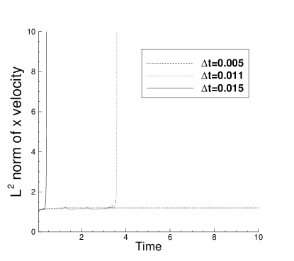
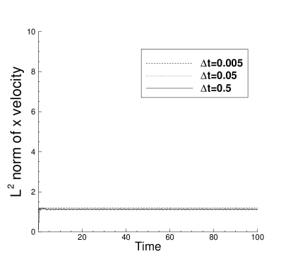
(a) (b)

Figure 5: Kovasznay flow: Time histories of the $L^{2}$ norm of the $x$ velocity obtained using several $\Delta t$ values using (a) the semi-implicit scheme of Dong2015clesobc , and (b) the current scheme.

The energy stability property of the current scheme (see Theorem 2.1) is conducive to the stability of computations. We observe that this scheme allows the use of fairly large or large time step sizes ($\Delta t$) in the simulations, at least for steady-state problems. In Table 1 we have listed the $L^{2}$ errors of the $x$ component of the steady-state velocity computed with different $\Delta t$ values, ranging from $\Delta t=0.001$ to $\Delta t=1.0$. In this set of simulations $C_{0}=0.01$ and two element orders ($10$ and $16$) have been used. We observe that for a given spatial resolution (element order) the computation result becomes less accurate or inaccurate when $\Delta t$ becomes too large. But the current scheme produces stable computations with all these $\Delta t$ values. In contrast, we observe that with the often-used semi-implicit type schemes, the computation will become unstable for moderately increased $\Delta t$ values. In Figure 5 we show the time histories of the $L^{2}$ norm of the $x$ component of the velocity computed using the semi-implicit scheme of Dong2015clesobc (Figure 5(a)) and the current scheme (Figure 5(b)). These results correspond to an element order $10$, and for the current scheme also $C_{0}=0.01$ in the simulations. The computation using the semi-implicit scheme blows up when $\Delta t$ is beyond about $0.01$, while the current scheme exhibits a different behavior and produces stable computations even with much larger $\Delta t$ values.

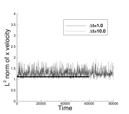
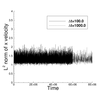
(a) (b)

Figure 6: Kovasznay flow: Time histories of the $L^{2}$ norm of the $x$ velocity obtained using several large $\Delta t$ values: (a) $\Delta t=1$ and $10$, (b) $\Delta t=100$ and $1000$. Results correspond to an element order 10 and $C_{0}=0.01$.

Figure 6 shows the time histories of the $L^{2}$ norm of the $x$ velocity of the Kovasznay flow obtained using the current scheme with several large time step sizes ranging from $\Delta t=1.0$ to $\Delta t=1000$. The element order is $10$ and $C_{0}=0.01$ in these simulations. While we cannot expect accuracy in these results because of the large $\Delta t$ values, the computations using the current scheme are nonetheless stable with these large $\Delta t$ for the Kovasznay flow.

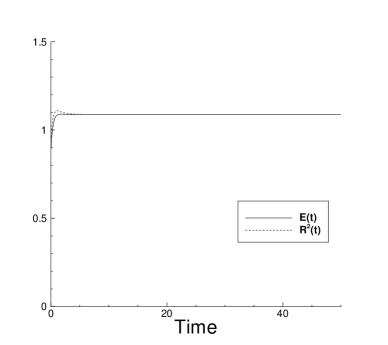
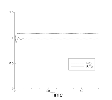
(a) (b)

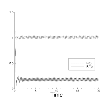
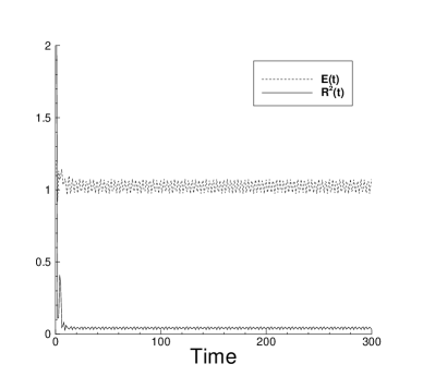
(c) (d)

Figure 7: Kovasznay flow: time histories of $E(t)$ and $R^{2}(t)$ obtained using several time step sizes: (a) $\Delta t=0.005$, (b) $\Delta t=0.01$, (c) $\Delta t=0.05$, (d) $\Delta t=1.0$. Results correspond to $C_{0}=0.01$ and an element order $10$ in the simulations.

In Figure 7 we plot the time histories of two variables: $E(t)$ defined by (6), and $[R(t)]^{2}$ computed by solving (11) from the current scheme. These two variables are supposed to be equal due to equation (7). With small $\Delta t$ values, the two quantities resulting from the computations are indeed the same, which is evident from the time histories obtained with $\Delta t=0.005$ in Figure (7)(a). The initial difference between the curves for $E(t)$ and $R^{2}(t)$ in Figure (7)(a) is due to the initial condition, because the zero initial velocity field is not compatible with the Dirichlet boundary condition (non-zero velocity) on the domain boundary. When $\Delta t$ becomes moderately large or very large, we can observe a difference between the computed $E(t)$ and $R^{2}(t)$, and the discrepancy between them becomes larger with increasing $\Delta t$ (Figures 7(b)-(d)). Both $E(t)$ and $R^{2}(t)$ fluctuate over time in the simulations using large $\Delta t$ values. While the computed $E(t)$ approximately stays at a constant mean level, $R(t)$ appears to be driven toward zero with very large $\Delta t$ in the simulations (Figure 7(d)). These results suggest that when $\Delta t$ becomes large the dynamical system consisting of equations (13a)–(13f) seems to be able to automatically adjust the $R(t)$ and the $\frac{R(t)}{\sqrt{E(t)}}$ levels. The term $\frac{R(t)}{\sqrt{E(t)}}$ places a control on the explicitly-treated nonlinear term in the Navier-Stokes equation (13a). With very large $\Delta t$ values, the system drives $\frac{R(t)}{\sqrt{E(t)}}$ toward zero, thus making the computation more stable or stabilizing the computation. This seems to be the mechanism by which the current scheme produces stable simulations with large $\Delta t$ for the Kovasznay flow.

3.3 Flow Past a Circular Cylinder in a Periodic Channel

In this section we investigate the flow past a circular cylinder inside a periodic channel, which is driven by a constant pressure gradient along the channel direction. We employ this problem to test the algorithm developed herein.

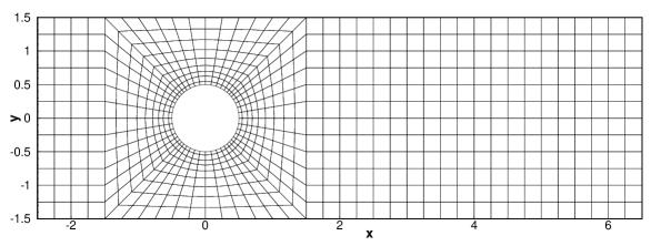
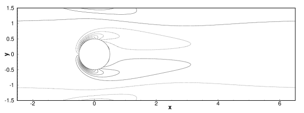
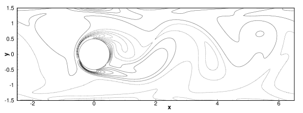
(a) (b) (c)

Figure 8: Cylinder flow in a periodic channel: (a) Mesh of $720$ quadrilateral elements. Vorticity contours at $\nu=0.01$ (b) and $\nu=0.005$ (c), with the flow driven by a normalized pressure gradient of $0.02$.

Consider a circular cylinder of diameter $D$ placed inside a horizontal channel occupying the domain $-2.5D\leqslant x\leqslant 6.5D$ and $-1.5D\leqslant y\leqslant 1.5D$, as depicted in Figure 8(a). The top and bottom of the domain ($y=\pm 1.5D$) are the channel walls. A pressure gradient is imposed along the $x$ direction to drive the flow. The flow domain and all the physical variables are assumed to be periodic in the horizontal direction at $x=-2.5D$ and $x=6.5D$. The center of the cylinder coincides with the origin of the coordinate system. This setting is equivalent to the flow past an infinite sequence of circular cylinders inside an infinitely long horizontal channel.

We use the cylinder diameter $D$ as the characteristic length scale. Let $\frac{\Delta P}{D}$ denote the pressure gradient (body force) that drives the flow along the $x$ direction, and let $g_{0}$ denote a unit body force magnitude. Then the non-dimensional body force in equation (1a) has the magnitude $|\mathbf{f}|=\frac{\Delta P}{g_{0}D}$ and points along the $x$ direction. We use $U_{0}=\sqrt{\frac{g_{0}D}{\rho_{f}}}$, where $\rho_{f}$ is the fluid density, as the characteristic velocity scale. All the length variables are normalized by $D$, and all velocity variables are normalized by $U_{0}$.

Figure 8(a) shows the spectral element mesh used to discretize the domain, which consists of $720$ quadrilateral elements. The element order has been varied between $2$ and $6$ in the simulations to test the effect of spatial resolutions on the simulation results. On the top and bottom channel walls, as well as on the cylinder surface, a no-slip condition is imposed on the velocity, that is, the boundary condition (3) with $\mathbf{w}=0$. In the horizontal direction (at $x/D=-2.5$ and $6.5$) periodic conditions are imposed for all the flow variables. Long-time simulations have been performed using the algorithm from Section 2 for a range of Reynolds numbers (or $\nu$) and the driving force $|\mathbf{f}|$. The simulation is started at a low Reynolds number with a zero initial velocity field at the very beginning. Then the Reynolds number is increased incrementally. A snapshot of the flow field from a lower Reynolds number is used as the initial condition in the simulation of the next larger Reynolds number. At each Reynolds number, a long-time simulation is performed (with typically $100$ flow-through times), such that the flow has reached a statistically stationary state for that Reynolds number and the initial condition will have no effect on the flow. A range of values for $\Delta t$ and $C_{0}$ have been tested in the simulations.

An overview of the flow features is provided by Figures 8(b) and (c), in which the contours of the instantaneous vorticity have been shown for two Reynolds numbers corresponding to $\nu=0.01$ and $\nu=0.005$ and a non-dimensional driving pressure gradient $|\mathbf{f}|=0.02$. The dashed curves denote negative vorticity values. With $\nu=0.01$ the flow reaches a steady state eventually. The pattern of the vorticity contours around the cylinder is typical of the cylinder flow DongKER2006 at low Reynolds numbers. Due to presence of the channel, we can also observe a certain level of vorticity distribution near the upper/lower channel walls above or below the cylinder. With $\nu=0.005$ an unsteady flow is observed, with periodical vortex shedding from the cylinder into the wake. Because of the periodicity in the horizontal direction, the vortices shed to the cylinder wake will re-enter the domain on the left side and influence the flow upstream of the cylinder. These upstream vortices interact with the cylinder, leading to more complicated dynamics and flow structures in the cylinder wake.

$\nu$	element order	mean-drag	rms-drag	mean-lift	rms-lift	driving force
$0.01$	$2$	$0.487$	$0$	$0$	$0$	$0.524$
	$3$	$0.527$	$0$	$0$	$0$	$0.524$
	$4$	$0.524$	$0$	$0$	$0$	$0.524$
	$5$	$0.524$	$0$	$0$	$0$	$0.524$
	$6$	$0.524$	$0$	$0$	$0$	$0.524$
$0.001$	$2$	$0.353$	$0.158$	$-8.90e-4$	$0.270$	$0.524$
	$3$	$0.519$	$0.269$	$-1.35e-3$	$2.83e-2$	$0.524$
	$4$	$0.530$	$0.277$	$-3.72e-4$	$1.36e-2$	$0.524$
	$5$	$0.526$	$0.280$	$1.62e-5$	$3.80e-3$	$0.524$
	$6$	$0.524$	$0.289$	$8.96e-5$	$1.64e-3$	$0.524$

Table 2: Effect of spatial resolution on the computed forces acting on channel/cylinder walls. Drag refers to the force in the $x$ direction and lift refers to the force in the $y$ direction. Driving force is the normalized total force driving the flow due to the imposed pressure gradient.

The effect of the spatial mesh resolution on the simulation results is demonstrated by Table 2. We have computed the total forces acting on the walls (sum of those on the cylinder surface and channel wall surfaces) from the simulations. This table lists the time-averaged mean drag (or drag if steady flow), root-mean-square (rms) drag, mean lift, and rms lift on the walls corresponding to a non-dimensionalized driving pressure gradient $\frac{\Delta P}{g_{0}D}=0.02$. Several element orders, ranging from $2$ to $6$, are tested in the simulations. The results for two Reynolds numbers corresponding to $\nu=0.01$ and $\nu=0.001$ have been included in the table, and they are obtained using $\Delta t=0.01$ in the simulations. The total driving force on the flow is $\frac{\Delta P}{g_{0}D}\times V_{\Omega}=0.02\times 26.2146\approx 0.524,$ where $V_{\Omega}=((6.5+2.5)\times(1.5+1.5)-\pi/4)\approx 26.2146$ is the normalized volume (or area) of the flow domain. At steady state or statistically stationary state of the flow, this driving force will be balanced by the total force exerted on the flow by the walls. This will give rise to a total mean drag acting on the walls with the same value as the total driving force. Therefore, we expect that the time-averaged mean drag (or the drag if steady flow) obtained from the simulations should be equal or close to the total driving force in the flow domain. This can be used to check the accuracy of the simulations. With very low element orders, we observe a discrepancy between the computed drag from the simulations and the expected value. As the element order increases in the simulations, this discrepancy decreases and becomes negligible or completely vanishes. For $\nu=0.01$, the computed drag becomes very close to the expected value for element order $3$, and with element orders $4$ and above the computed drag matches the expected value. For $\nu=0.001$, the difference between the computed mean-drag and the expected value becomes very small with element orders $5$ and above.

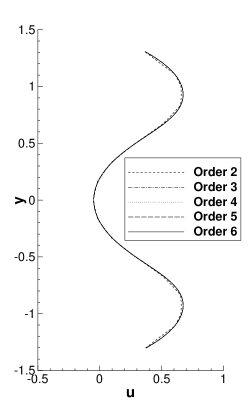
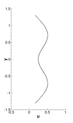
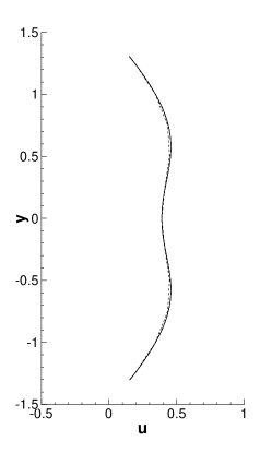
(a) (b) (c)

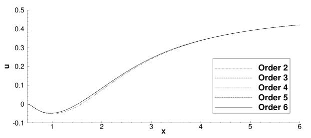
(d)

Figure 9: Comparison of stream-wise velocity profiles ($\nu=0.01$) computed using different element orders at downstream locations (a) $x/d=1.0$, (b) $x/d=3.0$, (c) $x/d=5.0$ and the velocity profiles along the centerline of domain (d) $y=0.0$. Results are obtained with $\Delta t=0.01$ and $C_{0}=1000$ in the simulations.

Figure 9 shows a comparison of the profiles of the steady-state stream-wise velocity along the cross-flow direction at several downstream locations $x/D=1$, $3$, and $5$, as well as along the centerline of the domain ($y=0$), for the Reynolds number corresponding to $\nu=0.01$ and with several element orders in the simulations. The total driving force in the domain is $0.524$. While some difference can be observed between the profile corresponding to element order $2$ and the other profiles, all the velocity profiles obtained with the element orders $3$ and above basically overlap with one another, suggesting the independence with respect to the spatial resolutions. In light of these observations, the majority of simulations reported below are performed using an element order $4$, and for higher Reynolds numbers the results corresponding to an element order $5$ are also employed in the simulations.

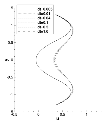
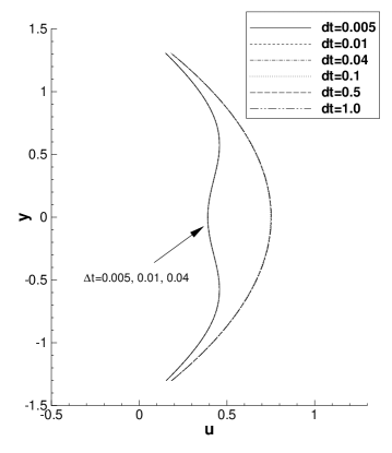
(a) (b)

Figure 10: Effect of the time step size $\Delta t$ ($\nu=0.01$): stream-wise velocity profiles at downstream locations (a) $x/D=1.0$ and (b) $x/D=5.0$ obtained with different time step sizes.

The effect of the time step size $\Delta t$ on the simulation results is illustrated by Figure 10, in which we compare the stream-wise velocity profiles along the $y$ direction at the downstream locations $x/D=1$ and $5$ obtained with time step sizes ranging from $\Delta t=0.005$ to $\Delta t=1.0$. These results are computed with an element order $4$ for the Reynolds number corresponding to $\nu=0.01$, and the total driving force is $0.524$ in the domain. The profiles obtained with time step sizes $\Delta t=0.04$ and smaller all overlap with one another. With larger $\Delta t$ values (e.g. $\Delta t=0.1$, $0.5$ and $1.0$), our method is also able to produce stable simulations at this Reynolds number. But the obtained velocity profiles exhibit a pronounced difference when compared with those computed using smaller $\Delta t$ values, indicating that these results are no longer accurate. From numerical experiments we observe that for steady-state flow problems the current method seems to be able to produce stable computations, even with very large $\Delta t$ values in the simulations, as have been shown here and in Section 3.2. For Reynolds numbers at which the flow is unsteady, despite the energy stability property (Theorem 2.1), we observe that in practice there is a restriction on the maximum $\Delta t$ that can be used in the simulations, at least with our current implementation of the scheme. The computation will become unstable when $\Delta t$ exceeds this value. For the results reported subsequently, the simulations are performed with $\Delta t=0.01$ for lower Reynolds numbers ($\nu\geqslant 0.005$), and $\Delta t=0.001$ for higher Reynolds numbers ($\Delta t=5E-4$ for the Reynolds number corresponding to $\nu=2\times 10^{-4}$).

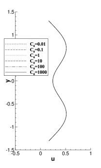
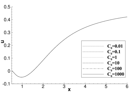
(a) (b)

Figure 11: $C_{0}$ effect: Comparison of stream-wise velocity profiles ($\nu=0.01$) at (a) $x=3.0$ and (b) along the centerline, obtained using a range of $C_{0}$ values in the algorithm.

The constant $C_{0}$ in the current algorithm has been observed to influence the accuracy of the steady-state solution for the Kovasznay flow in the previous section. Whether $C_{0}$ affects the accuracy of results for the current problem has also been studied, and we observe no apparent effect of the $C_{0}$ value on the forces and the flow field distributions. For the Reynolds number corresponding to $\nu=0.01$ and a total driving force $0.524$, we have performed simulations with the $C_{0}$ constant ranging from $C_{0}=0.01$ to $C_{0}=1000$ in the algorithm. The computed forces on the cylinder/channel walls from all these simulations match the total force imposed to drive the flow. Figure 11 compares the stream-wise velocity profiles at the downstream location $x/D=3$ and along the centerline of the domain ($y=0$) computed using different $C_{0}$ values in the current algorithm. The results correspond to an element order $4$ and time step size $\Delta t=0.01$ in the simulations. The velocity profiles for different cases exactly overlap with one another, suggesting that the computed velocity field is not sensitive to $C_{0}$ in the simulations. In the discussions of subsequent results, we employ a value $C_{0}=1000$ in the simulations unless otherwise specified.

$\nu$	mean-drag	rms-drag	mean-lift	rms-lift	Pressure Gradient	Driving Force
$0.01$	$0.131$	$0$	$0$	$0$	$0.005$	$0.131$
	$0.262$	$0$	$0$	$0$	$0.01$	$0.262$
	$0.524$	$0$	$0$	$0$	$0.02$	$0.524$
	$0.787$	$0$	$0$	$0$	$0.03$	$0.786$
	$1.049$	$0$	$0$	$0$	$0.04$	$1.049$
	$1.311$	$0$	$0$	$0$	$0.05$	$1.311$
$0.002$	$0.131$	$0.0105$	$9.64e-5$	$3.17e-4$	$0.005$	$0.131$
	$0.264$	$0.0519$	$1.97e-5$	$8.79e-4$	$0.01$	$0.262$
	$0.529$	$0.150$	$-9.10e-5$	$3.77e-3$	$0.02$	$0.524$
	$0.793$	$0.277$	$8.85e-5$	$8.82e-3$	$0.03$	$0.786$
	$1.059$	$0.427$	$-4.77e-4$	$1.45e-2$	$0.04$	$1.049$
	$1.324$	$0.574$	$2.35e-4$	$2.22e-2$	$0.05$	$1.311$

Table 3: Comparison of the forces on the cylinder/channel walls from the simulations and the imposed pressure gradient and total driving force.

We have varied the magnitude of the driving pressure gradient systematically ranging from $\frac{\Delta P}{g_{0}D}=0.005$ to $0.05$, and carried out simulations corresponding to each of the force values. In Table 3 we list the drag and lift on the walls obtained from the simulations for two fixed Reynolds numbers corresponding to $\nu=0.01$ and $\nu=0.002$. The imposed pressure gradient and the total driving force in the flow domain have also been shown. These results are obtained with an element order $4$ and a time step size $\Delta t=0.01$ in the simulations. Note that physically the mean drag from the simulations is expected to match the imposed total driving force. At the lower Reynolds number ($\nu=0.01$) the computed mean drag on the walls is essentially the same as the total driving force for different cases. At the higher Reynolds number ($\nu=0.002$) the computed mean-drag values also agree well with the driving forces. The discrepancy is less than $1\%$ for the range of driving forces considered here. The mean lift is zero or essentially zero, and the rms lift is also observed to be small.

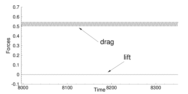
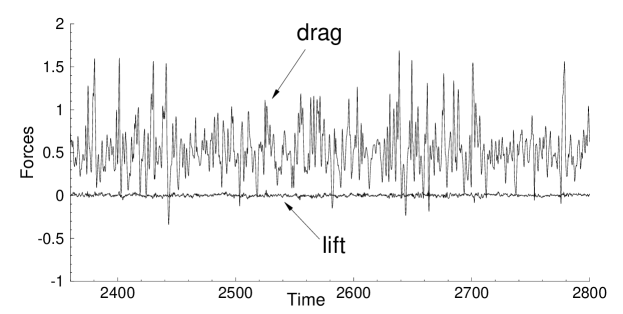
(a) (b)

Figure 12: Time histories of the drag and lift on the cylinder/channel walls for (a) $\nu=0.005$ and (b) $\nu=0.001$. The total driving force in the domain is $0.524$.

Figure 12 shows a window of the time histories of the drag and lift on the domain walls at two Reynolds numbers corresponding to $\nu=0.005$ and $\nu=0.001$, with a non-dimensional driving force $0.524$ in the domain. Periodic vortex shedding behind the cylinder can be observed at $\nu=0.005$ (see Figure 8(c) for the vorticity distribution), resulting in a periodic drag signal fluctuating about a constant mean value. As the viscosity decreases, vortices shed to the cylinder wake persist downstream and can be observed to re-enter the domain through the left boundary. The interactions between these upstream vortices and the cylinder cause the vortex shedding from the cylinder and the forces acting on the walls to become highly irregular. At $\nu=0.001$ one can observe chaotic fluctuations in the time histories of the drag and lift on the channel/cylinder walls (Figure 12(b)). Because of the confinement effect of the channel, the total lift acting on the domain walls appears quite insignificant, and it does not exhibit the large fluctuations as typically observed in the flow past a cylinder in an open domain (see e.g. DongKER2006 ; DongTK2008 ).

$\nu$	mean-drag	rms-drag	mean-lift	rms-lift	driving force
$0.02$	$0.524$	$0.0$	$0.0$	$0.0$	$0.524$
$0.01$	$0.524$	$0.0$	$0.0$	$0.0$	$0.524$
$0.005$	$0.525$	$0.0158$	$-5.30e-8$	$3.87e-4$	$0.524$
$0.00333$	$0.526$	$0.0760$	$2.69e-4$	$1.00e-3$	$0.524$
$0.002$	$0.529$	$0.150$	$-9.10e-5$	$3.77e-3$	$0.524$
$0.001$	$0.530$	$0.277$	$-3.72e-4$	$1.36e-2$	$0.524$
$0.0005$	$0.524$	$0.403$	$3.67e-4$	$3.73e-2$	$0.524$
$0.0002$	$0.523$	$0.590$	$-6.85e-4$	$4.35e-2$	$0.524$

Table 4: Forces on cylinder/channel walls obtained with different fluid viscosities. Simulations are performed with an element order $5$ for $\nu=0.0002$ and $4$ for the other $\nu$ values.

We have simulated this flow problem for a range of Reynolds numbers corresponding to viscosities ranging from $\nu=0.02$ to $\nu=0.0002$, with the total driving force fixed at $0.524$ (corresponding to a non-dimensional pressure gradient $0.02$). Table 4 lists the mean and rms forces acting on the walls obtained from the simulations corresponding to different Reynolds numbers. In the simulations the element order is $5$ for the case $\nu=0.0002$ and $4$ for the other cases. As expected, the mean drag values obtained from the simulations are very close to or the same as the driving force for different Reynolds numbers, indicating that the method has captured the flow quite accurately. The rms drag is observed to increase significantly with increasing Reynolds number (decreasing $\nu$), while the rms lift remains insignificant for the range of Reynolds numbers considered here.

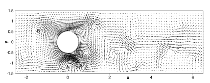
(a) (b)

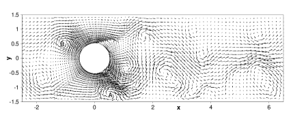
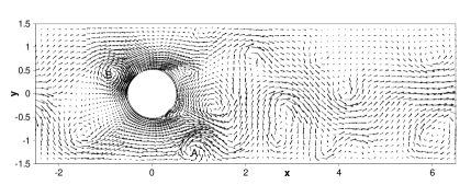
(c) (d)

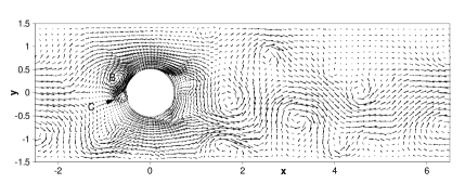
(e) (f)

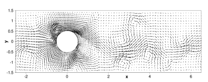
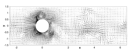
(g) (h)

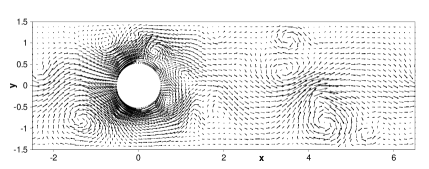
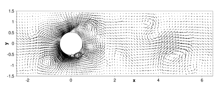
(i) (j)

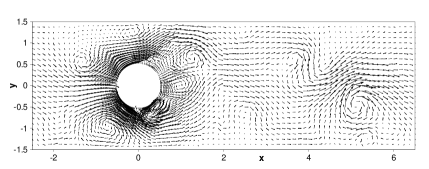
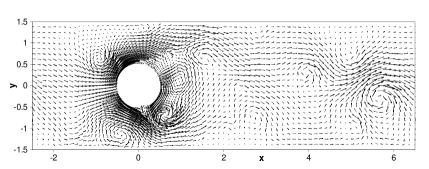
(k) (l)

Figure 13: Temporal sequence of snapshots of the velocity fields ($\nu=0.0002$, total driving force $0.524$) at time (a) $t=3941.5$, (b) $t=3942$, (c) $t=3942.5$, (d) $t=3943$, (e) $t=3943.5$, (f) $t=3944$, (g) $t=3944.5$, (h) $t=3945$, (i) $t=3945.5$, (j) $t=3946$, (k) $t=3946.5$, (l) $t=3947$. Velocity vectors are plotted on every eighth quadrature points in each direction within each element.

The dynamics of this flow is illustrated by the temporal sequence of snapshots of the velocity fields shown in Figure 13 for the Reynolds number corresponding to $\nu=0.0002$. In addition to the multitude of vortices permeating the cylinder wake, the prominent feature of this flow lies in the upstream vortices and their interactions with the cylinder. Such interactions induce complicated dynamic features. Some upstream vortices can simply squeeze through the gap between the cylinder and the channel wall and move downstream into the wake, as is illustrated by the vortex marked by the symbol “A” in Figures 13(a)-(d). However, the interaction between the vortex and the cylinder can be more complicated. This is illustrated by the vortex marked by “B” in Figures 13(a)-(g). The incoming vortex B appears to directly collide with the cylinder (Figures 13(a)-(d)). Upon impact, a new vortex (marked by “C”) is spawned near the front of the cylinder due to the strong shear layer generated (Figure 13(e)). This causes the subsequent interactions even more dynamic. Other processes (such as the coalescence of vortices) can also be observed in the wake of the cylinder (see Figures 13(h)-(j)).

	Newton-solver time/step (seconds)	Total wall time/step (seconds)
Current scheme	$0.00198$	$0.0965$
Semi-implicit scheme Dong2015clesobc	–	$0.0505$

Table 5: Computational cost: comparison of wall time per time step (single processor) between the current scheme and the semi-implicit scheme of Dong2015clesobc for the flow past a cylinder in a periodic channel with $\nu=0.0002$ (element order $5$). The total wall time contains the Newton solver time for the current scheme.

Finally we look into the computational cost of the scheme developed in this work. For the cylinder flow problem in a periodic channel we have monitored the wall clock time per time step in the simulations. In Table 5 we list the typical wall time it takes the current scheme to compute one time step (in seconds) on a single processor for the Reynolds number corresponding to $\nu=0.0002$, as well as the wall time spent in the Newton solver for solving the scalar equation (37). These wall-time numbers are collected on a Linux cluster in the authors’ institution. The cost of the Newton solver is insignificant, accounting for about $2\%$ of the total cost of the current scheme per time step. For comparison the table also includes the wall clock time per time step of the semi-implicit scheme from Dong2015clesobc . The current scheme requires the solution of two pressure fields $p_{1}^{n+1}$ and $p_{2}^{n+1}$ and two velocity fields $\mathbf{u}_{1}^{n+1}$ and $\mathbf{u}_{2}^{n+1}$, which involves approximately twice as many operations as the semi-implicit scheme. The computational cost of the current scheme is roughly twice that of the semi-implicit scheme, as is evident from Table 5.

4 Concluding Remarks

We have presented an algorithm for approximating the incompressible Navier-Stokes equations based on an auxiliary variable associated with the total energy of the system. This auxiliary variable is a scalar number (not a field function), and a dynamic equation for this variable has been introduced. This leads to a reformulated equivalent system consisting of the modified incompressible Navier-Stokes equations and the dynamic equation for the auxiliary variable. The numerical scheme for the reformulated system satisfies a discrete energy stability property in terms of a modified energy. Within each time step, the algorithm requires the computations in a de-coupled fashion of (i) two pressure variables $p_{1}^{n+1}$ and $p_{2}^{n+1}$, (ii) two velocity variables $\mathbf{u}_{1}^{n+1}$ and $\mathbf{u}_{2}^{n+1}$, and (iii) the scalar auxiliary variable. Computing the pressure variables and the velocity variables involves only the usual Poisson equations and Helmholtz equations with constant coefficient matrices. Computing the auxiliary variable requires the solution of a nonlinear scalar algebraic equation based on the Newton’s method. The cost for the Newton solution is insignificant and essentially negligible (accounting for roughly $2\%$ of the total cost per time step), because the nonlinear equation is about a scalar number, not a field function.

The algorithm has been implemented based on a $C^{0}$ spectral element technique in the current work, and several numerical examples have been presented to test its accuracy and performance. The method is observed to exhibit a second-order convergence rate in time and an exponential convergence rate in space (for smooth field solutions). It can capture the flow field accurately when the time step size is not too large. The method also allows the use of large time step sizes in computations for steady flow problems, and stable simulation results can be produced.

The presented scheme has an attractive energy stability property, and it can be implemented in an efficient fashion. The algorithm involves only constant and time-independent coefficient matrices in the resultant linear algebraic systems, which is unlike other energy-stable schemes for Navier-Stokes equations (see e.g. SimoA1994 ; LabovskyLMNR2009 ; DongS2010 , among others). This algorithm can serve as an alternative to the semi-implicit schemes for production simulations of incompressible flows and flow physics studies.

References

- [1] H. Abels, H. Garcke, and G. Grün. Thermodynamically consistent, frame indifferent diffuse interface models for incompressible two-phase flows with different densities. Mathematical Models and Methods in Applied Sciences, 22:1150013, 2012.
- [2] D.L. Brown, R. Cortez, and M.L. Minion. Accurate projection methods for the incompressible Navier-Stokes equations. J. Comput. Phys., 168:464–499, 2001.
- [3] H. Chen, S. Sun, and T. Zhang. Energy stability analysis of some fully discrete numerical schemes for incompressible navier-stokes equations on staggered grids. Journal of Scientific Computing, 75:427–456, 2018.
- [4] L. Chen, J. Shen, and C.J. Xu. A unstructured nodal spectral-element method for the navier-stokes equations. Communications in Computational Physics, 12:315–336, 2012.
- [5] A.J. Chorin. Numerical solution of the Navier-Stokes equations. Math. Comput., 22:745–762, 1968.
- [6] S. Dong. Direct numerical simulation of turbulent Taylor-Couette flow. J. Fluid Mech., 587:373–393, 2007.
- [7] S. Dong. Evidence for internal structures of spiral turbulence. Physical Review E, 80:067301, 2009.
- [8] S. Dong. A convective-like energy-stable open boundary condition for simulations of incompressible flows. Journal of Computational Physics, 302:300–328, 2015.
- [9] S. Dong. Multiphase flows of N immiscible incompressible fluids: a reduction-consistent and thermodynamically-consistent formulation and associated algorithm. Journal of Computational Physics, 361:1–49, 2018.
- [10] S. Dong, G.E. Karniadakis, A. Ekmekci, and D. Rockwell. A combined direct numerical simulation-particle image velocimetry study of the turbulent near wake. J. Fluid Mech., 569:185–207, 2006.
- [11] S. Dong and J. Shen. An unconditionally stable rotational velocity-correction scheme for incompressible flows. Journal of Computational Physics, 229:7013–7029, 2010.
- [12] S. Dong and J. Shen. A time-stepping scheme involving constant coefficient matrices for phase field simulations of two-phase incompressible flows with large density ratios. Journal of Computational Physics, 231:5788–5804, 2012.
- [13] S. Dong, G.S. Triantafyllou, and G.E. Karniadakis. Elimination of vortex streets in bluff body flows. Phys. Rev. Lett., 100:204501, 2008.
- [14] S. Dong and X. Zheng. Direct numerical simulation of spiral turbulence. J. Fluid Mech., 668:150–173, 2011.
- [15] J.L. Guermond, P. Minev, and J. Shen. An overview of projection methods for incompressible flows. Comput. Methods Appl. Mech. Engrg., 195:6011–6045, 2006.
- [16] J.L. Guermond and J. Shen. A new class of truly consistent splitting schemes for incompressible flows. J. Comput. Phys., 192:262–276, 2003.
- [17] B. Hyoungsu and G.E. Karniadakis. Subiteration leads to accuracy and stability enhancements of semi-implicit schemes for the navier-stokes equations. Journal of Computational Physics, 230:4384–4402, 2011.
- [18] N. Jiang, M. Mohebujjaman, L.G. Rebholz, and C. Trenchea. An optimally accurate discrete regularization for second order timestepping methods for navier-stokes equations. Comput. Methods Appl. Mech. Engrg., 310:388–405, 2016.
- [19] G.E. Karniadakis, M. Israeli, and S.A. Orszag. High-order splitting methods for the incompressible Navier-Stokes equations. J. Comput. Phys., 97:414–443, 1991.
- [20] G.E. Karniadakis and S.J. Sherwin. Spectral/hp element methods for computational fluid dynamics, 2nd edn. Oxford University Press, 2005.
- [21] J. Kim and P. Moin. Application of a fractional-step method to incompressible Navier-Stokes equations. J. Comput. Phys., 59:308–323, 1985.
- [22] L.I.G. Kovasznay. Laminar flow behind a two-dimensional grid. Proc. Cambridge Phil. Soc., 44:58, 1948.
- [23] A.G. Kravchenko and P. Moin. Numerical studies of flow over a circular cylinder at Re. Physics of Fluids, 12:403–417, 2000.
- [24] A. Labovsky, W.J. Layton, C.C. Manica, M. Neda, and L.G. Rebholz. The stabilized extrapolated trapezoidal finite-element method for the Navier-Stokes equations. Comput. Methods Appl. Mech. Engrg., 198:958–974, 2009.
- [25] J.-G. Liu, J. Liu, and R.L. Pego. Stability and convergence of efficient Navier-Stokes solvers via a commutator estimate. Comm. Pure Appl. Math., LX:1443–1487, 2007.
- [26] X. Ma, C.S. Karamanos, and G.E. Karniadakis. Dynamics and low-dimensionality of a turbulent near wake. J. Fluid Mech., 410:29–65, 2000.
- [27] B. Sanderse. Energy-conserving runge-kutta methods for the incompressible navier-stokes equations. J. Comput. Phys., 233:100–131, 2013.
- [28] D. Serson, J.R. Meneghini, and S.J. Sherwin. Velocity-correction schemes for the incompressible navier-stokes equations in general coordinate systems. Journal of Computational Physics, 316:243–254, 2016.
- [29] J. Shen. On error estimate of projection methods for Navier-Stokes equations: first-order schemes. SIAM J. Numer. Anal., 29:57–77, 1992.
- [30] J. Shen, J. Xu, and J. Yang. The scalar auxiliary variable (sav) approach for gradient flows. Journal of Computational Physics, 353:407–416, 2018.
- [31] S.J. Sherwin and G.E. Karniadakis. A triangular spectral element method: applications to the incompressible navier-stokes equations. Comput. Meth. Appl. Mech. Engrg., 123:189–229, 1995.
- [32] J.C. Simo and F. Armero. Unconditional stability and long-term behavior of transient algorithms for the incompressible Navier-Stokes and Euler equations. Comput. Methods Appl. Mech. Engrg., 111:111–154, 1994.
- [33] R. Temam. Sur l’approximation de la solution des equations de Navier-Stokes par la methods des pas fractionnaires ii. Arch. Ration. Mech. Anal., 33:377–385, 1969.
- [34] C.J. Xu and R. Pasquetti. On the efficiency of semi-implicit and semi-lagrangeian spectral methods for the calculation of incompressible flows. International Jurnal for Numerical Methods in Fluids, 35:319–340, 2001.
- [35] P. Yue, J.J. Feng, C. Liu, and J. Shen. A diffuse-interface method for simulating two-phase flows of complex fluids. J. Fluid Mech., 515:293–317, 2004.
- [36] X. Zheng and S. Dong. An eigen-based high-order expansion basis for structured spectral elements. Journal of Computational Physics, 230:8573–8602, 2011.