Density functional theory beyond the Born-Oppenheimer approximation: accurate treatment of the ionic zero-point motion

Abstract

We introduce a method to carry out zero-temperature calculations within density functional theory (DFT) but without relying on the Born-Oppenheimer (BO) approximation for the ionic motion. Our approach is based on the finite-temperature many-body path-integral formulation of quantum mechanics by taking the zero-temperature limit and treating the imaginary-time propagation of the electronic variables in the context of DFT. This goes beyond the familiar BO approximation and is limited from being an exact treatment of both electrons and ions only by the approximations involved in the DFT component. We test our method in two simple molecules, H₂ and benzene. We demonstrate that the method produces a difference from the results of the BO approximation which is significant for many physical systems, especially those containing light atoms such as hydrogen; in these cases, we find that the fluctuations of the distance from its equilibrium position, due to the zero-point-motion, is comparable to the interatomic distances. The method is suitable for use with conventional condensed matter approaches and currently is implemented on top of the periodic pseudopotential code SIESTA.

I Introduction

The physical properties of solids and molecules can be determined computationally by generating many realizations of the system, described by its electronic and ionic degrees of freedom, and sampling the quantities of interest during the numerical simulation. A common approach is to separate the electronic and ionic motion, known as the Born-Oppenheimer (BO) approximation, justified by the large mass difference between electrons and ions and the large separation between electronic energy eigenvalues. Within the BO approximation, the ions may be treated as classical or quantum mechanical particles; in either case, an effective interaction potential between ions can be obtained by solving the electronic problem for each instantaneous ionic configuration, and then using molecular dynamicsPayne et al. (1992); Marx and Hutter (2009) or Monte Carlo simulations to generate configurations for sampling the system’s properties.

In several situations, a quantum mechanical treatment of the ionic degrees of freedom is mandatory. A case in point is that of liquid and solid helium Ceperley (1995a), ⁴He, or helium films on various substratesPierce and Manousakis (1998); *Pierce-second-layer; *Pierce-solid; *Pierce-corrugations; *Ceperley-Manousakis. In these situations, there are several approaches for capturing the effect of ionic motion by path-integral Monte Carlo (PIMC), with the electronic degrees of freedom integrated out through the effective interaction they produce between ions within the BO approximation. One can then sample the atomic configurations using PIMC, as in the original work of Pollock and CeperleyPollock and Ceperley (1984). In the case of ⁴He it has been deemed reasonable to ignore the electronic degrees of freedom altogether at very low temperature, because ⁴He is a closed-shell atom in which the first excited atomic state is several eV above the ground state. At low temperature, where the average kinetic energy of the atoms due to their zero-point-motion (ZPM) is of order $10^{-3}$ eV per atom, they behave as “elementary” particles, that is, they do not exhibit their internal structure as it is extremely unlikely to become excited through such low-energy collisions. The effective interatomic potential in this case can be simply modeled by a Lennard-Jones type interaction. Similar empirical-potential and tight-binding path-integral approaches have been applied in solids Ramírez and Herrero (1993); Kaxiras and Guo (1994); Noya et al. (1996); Herrero and Ramirez (2014); Ramírez et al. (2006). In more general situations, the disentanglement of the electronic and ionic degrees of freedom might not be possibleMcMahon et al. (2012); Pisana et al. (2007); Vidal-Valat et al. (1992); Bunker (1977); Coxon and Hajigeorgiou (1991); Schwenke (2001) and accurate approaches have been developed to treat the full electron-ion problem Tubman et al. (2014); Mitroy et al. (2013); Wolniewicz (1995, 1993); Chen and Anderson (1995); Yang et al. (2015); Webb et al. (2002); Chakraborty et al. (2008); Kylänpää and Rantala (2010). With these approaches, however, it is presently difficult to go beyond smaller systems. A recent development is a multi-component extension of the density functional theory Kohn and Sham (1965) (DFT) which treats both electronic and nuclei degrees of freedom in the density functionalKreibich and Gross (2001); Kreibich et al. (2008). The construction of the electron-ion density functional is a difficult problem however and approximations, including the BO approximation, are employed in practice Lüders et al. (2005); Marques et al. (2005).

A useful and general approach, that has proven quite satisfactory in many applications, is to treat only the electrons within density functional theory Kohn and Sham (1965) (DFT). This approach can serve as the basis for path-integral simulations of ionic motion, where the problem of a quantum mechanical treatment of ions maps to a classical problem of ring-polymers Barker (1979); Chandler and Wolynes (1981) interacting by means of the electronic stationary-state energy for the instantaneous atomic configuration of each bead of the ring polymer Cao and Berne (1993); Marx and Parrinello (1994, 1996); Benoit et al. (1998); Marx et al. (1999); Morrone and Car (2008); Städele and Martin (2000); Johnson and Ashcroft (2000); Miller III and Manolopoulos (2005); Ceriotti et al. (2016); Habershon et al. (2013). This formulation is within the BO approximation and ignores the role of the electronic excitations for a given ring-polymer configuration which contributes to the path integral over atomic coordinates.

Here, working in the zero-temperature limit, we introduce an approach that goes beyond the BO approximation and is exact in the context of the method chosen to solve the electronic problem. We choose DFT for handling the electronic degrees of freedom, although any other approximation with a tractable time-evolution of the electronic wavefunctions can also be implemented in our method. As far as including the quantum fluctuations of the atomic positions is concerned, we use the path-integral formulation. In particular, we find the exact eigenstate of the electronic evolution operator of the entire effective ring-polymer which represents the atomic space-time path in imaginary time. This becomes possible because we use the evolution operator within the DFT formulation that reduces to an effective single-particle-like evolution, which has to be solved self-consistently. This yields a self-consistent space-time electronic density, thus incorporating “exactly” within DFT the imaginary-time correlations of the density. As a result, our method introduces the concept of an electronic super-wavefunction which is a space-time-correlated state of the electrons in the entire pseudo-ring-polymer representing the space-time Feynman path of the atomic configuration in Euclidean (imaginary) time. Thus, our choices allow us to effectively include the contribution of all virtual electronic excitations. Finally, as in other quantum simulation methods, our method employs a periodic supercell which includes all the atoms for single molecules while in the case of crystalline solids it must involve large enough number of primitive unit cells to limit the role of finite-size effects.

To test the method, we apply it to two model systems, the hydrogen and the benzene molecules. We find that the size of root-mean-square (rms) radius due to the ZPM of the hydrogen atom is comparable to typical interatomic distances. In this case, we expect that the evolution of the electronic states and the ionic motion should be correlated. We also find that the energy difference between our method and BO approximation-based approaches to this problem is approximately 5 meV per atom even in the hydrogen molecule that has a wide energy gap between occupied and unoccupied electronic states. An energy difference on this scale can be important in properly describing low-temperature properties and phases of materials, such as the determination of a charge density wave or solidification of a system which contains hydrogen or other light atoms. Furthermore, since life is a subtle phenomenon which is severely affected when the average energy per atom of the biological system is raised by $\sim 1$ meV ($\sim 10^{\circ}$K), 5 meV per atom is an energy scale which may have dramatic effects in living matter. Since biological systems contain plenty of hydrogen atoms that participate in important hydrogen-bonded structures, their microscopic treatment might benefit from the method presented here.

The paper is organized as follows. In the following Section we present the method and in Sec. III its implementation. In Sec. IV we apply the method to two prototypical smalls systems, the H₂ and the benzene molecules, and present our conclusions based on these results in Sec. V.

II Description of the method

The method is described in three steps: first, the propagation in imaginary-time within the DFT Hamiltonian, next the many-body path integral form of the partition function within the DFT treatment of the electronic degrees of freedom, and finally the extraction of the exact ground-state of the combined ion-electron system within the DFT scheme.

II.1 DFT imaginary-time propagation

In real-time time-dependent DFT (TDDFT) the time-dependent electronic density is obtained as the solution to the equation:

$$\hat{\cal H}^{\rm sp}_{\{\vec{R}\}}[n(t),\vec{r}]|\psi_{l}(t)\rangle = {\rm i}\hbar\partial_{t}|\psi_{l}(t)\rangle,$$ (1)

starting from a given initial set of orbitals $|\psi_{n}(0)\rangle$. Here, for simplicity, the adiabatic approximation is used, that is, the electronic single-particle hamiltonian $\hat{\cal H}^{\rm sp}_{\{\vec{R}\}}$ is a functional of the instantaneous electronic density $n(\vec{r},t)=\sum_{l}\psi_{l}^{*}(\vec{r},t)\psi_{l}(\vec{r},t)$. Namely, the single-particle hamiltonian consists of the kinetic energy, the external potential for the electrons $V_{\rm ext}(\vec{r}-\vec{R}_{I})$, the Hartree potential $V_{H}[n,\vec{r}]$ and the exchange-correlation potential $V_{xc}[n,\vec{r}]$ terms:

$$\hat{\cal H}^{\rm sp}_{\{\vec{R}\}}[n,\vec{r}] = -{{\hbar^{2}}\over{2m_{e}}}\nabla_{\vec{r}}^{2}+\sum_{I=1}^{N_{\rm ion}}V_{\rm ext}(\vec{r}-\vec{R}_{I})$$ (2)

$$+ V_{H}[n,\vec{r}]+V_{xc}[n,\vec{r}],$$

$$V_{H}[n,\vec{r}] = e^{2}\int\frac{n(\vec{r}\mkern 2.0mu\vphantom{r}^{\prime})}{|\vec{r}-\vec{r}\mkern 2.0mu\vphantom{r}^{\prime}|}d^{3}r^{\prime}.$$ (3)

The dependence of the hamiltonian on ionic coordinates, collectively denoted by $\{\vec{R}\}$, is indicated by the subscript. The iterative solution to the analytically continued TDDFT equations to imaginary time

$$\hat{\cal H}^{\rm sp}_{\{\vec{R}\}}[n(\tau),\vec{r}]|\psi_{l}(\tau)\rangle=-\partial_{\tau}|\psi_{l}(\tau)\rangle,$$ (4)

where $\tau={\rm i}t/\hbar$, can be formally written as

$$|\psi_{l}(\tau)\rangle=\hat{\cal T}\exp\left[-\int_{0}^{\tau}\hat{\cal H}_{\{\vec{R}\}}^{\rm sp}[n(\tau^{\prime}),\vec{r}]d\tau^{\prime}\right]|\psi_{l}(0)\rangle,$$ (5)

where $\hat{\cal T}$ is the time-ordering operator. It is straightforward to show that starting from a complete and orthonormal set of initial states $|\psi_{l}(0)\rangle$, after infinite imaginary-time $\tau$ (in practice longer than $\hbar/\Delta\epsilon$, where $\Delta\epsilon$ is the minimum energy-level spacing) the solutions to these equations are the correct static DFT eigenstates Chin et al. (2009); Mendoza et al. (2014). The evolution under imaginary time projects the lowest energy eigenstate which is not orthogonal to the initial state. Since we start from a state characterized by definite quantum numbers, which include the wave-vector $\vec{k}$ and band index, the minimum energy spacing is not necessarily zero in the subspace defined by fixing these quantum numbers.

II.2 Finite temperature formulation

We next wish to calculate the average expectation value of a given observable $\hat{\cal O}$ as usual

$$\langle\langle\hat{\cal O}\rangle\rangle={{{\rm Tr}(\hat{\rho}\hat{\cal O})}\over{{\rm Tr}(\hat{\rho})}}$$ (6)

where the trace refers to averaging over all possible ionic configurations $\{\vec{R}\}$ and over a complete basis of electronic states. The total contribution to the statistical density matrix $\hat{\rho}$ is given as $\hat{\rho}=\exp(-\beta\hat{\cal H})$, where $\hat{\cal H}$ is the many-body hamiltonian operator for the ion-electron wavefunction. The average $\langle\langle\hat{\cal O}\rangle\rangle$ can be carried out using Feynman paths in imaginary timeFeynman (1972); Feynman et al. (2010), by writing

$${\rm e}^{-\beta\hat{\cal H}}={\rm e}^{-\Delta\tau\hat{\cal H}}{\rm e}^{-\Delta\tau\hat{\cal H}}...{\rm e}^{-\Delta\tau\hat{\cal H}},$$ (7)

where $K\Delta\tau=\beta$ ($K$ is the number of terms in the above product). We can introduce complete sets of states, namely,

$$\int\prod_{I=1}^{N_{\rm ion}}d\vec{R}_{I}^{(j)}|\vec{R}_{I}^{(j)}\rangle\langle\vec{R}_{I}^{(j)}|\sum_{n_{j}}|\Psi_{n_{j}}\rangle\langle\Psi_{n_{j}}|=\hat{1},$$ (8)

$K-1$ times, between each $j$th pair of exponentials. We have chosen the electronic states to be the ion-independent states $|\Psi_{n_{j}}\rangle$, which denote $N_{\rm ele}\times N_{\rm ele}$ Slater determinants of all possible selections of $N_{\rm ele}$ orbitals from the entire single-particle Hilbert space spanned by a suitable complete single-particle basis:

$$\sum_{n_{j}}|\Psi_{n_{j}}\rangle\langle\Psi_{n_{j}}| = \hat{1}_{\rm ele},$$ (9)

Applying the Trotter expansion for the ionic coordinates and the ionic kinetic energy operator and integrating out intermediate electronic states we get:

$$Z = \int{\cal D}\vec{\cal R}{\rm e}^{-{\cal S}_{E}}\sum_{n_{1}}\langle\Psi_{n_{1}}|\exp\left(-\Delta\tau\hat{\cal H}_{\{\vec{R}^{(1)}\}}\right)\sum_{n_{2}}|\Psi_{n_{2}}\rangle\langle\Psi_{n_{2}}|\exp\left(-\Delta\tau\hat{\cal H}_{\{\vec{R}^{(2)}\}}\right)$$ (10)

$$\sum_{n_{3}}|\Psi_{n_{3}}\rangle\langle\Psi_{n_{3}}|\ldots\exp\left(-\Delta\tau\hat{\cal H}_{\{\vec{R}^{(K)}\}}\right)|\Psi_{n_{1}}\rangle$$

$$= \int{\cal D}\vec{\cal R}{\rm e}^{-{\cal S}_{E}}\sum_{n_{1}}\langle\Psi_{n_{1}}|\prod_{j=1}^{K}\exp\left(-\Delta\tau\hat{\cal H}_{\{\vec{R}^{(j)}\}}\right)|\Psi_{n_{1}}\rangle,$$

$$\langle\langle\hat{\cal O}\rangle\rangle = {1\over Z}\int{\cal D}\vec{\cal R}\hskip 7.22743pt{\rm e}^{-{\cal S}_{E}}\times\sum_{n_{1}}\langle\Psi_{n_{1}}|\hat{\cal O}\prod_{j=1}^{K}\exp\left(-\Delta\tau\hat{\cal H}_{\{\vec{R}^{(j)}\}}\right)|\Psi_{n_{1}}\rangle,$$ (11)

$${\cal D}\vec{\cal R} \equiv \prod_{j=1}^{K}\prod_{I=1}^{N_{\rm ion}}d\vec{R}_{I}^{(j)},$$ (12)

$${\cal S}_{E} \equiv \sum_{I=1}^{N_{\rm ion}}\sum_{j=1}^{K}{M_{I}\over{2\hbar^{2}\Delta\tau}}\left|\vec{R}_{I}^{(j+1)}-\vec{R}_{I}^{(j)}\right|^{2},$$ (13)

where $Z$ is the partition function $Z={\rm Tr}[e^{-\beta\hat{\cal H}}]$ and $\hat{\cal H}_{\{\vec{R}^{(j)}\}}$ is the electronic hamiltonian at ionic positions collectively denoted as $\{\vec{R}^{(j)}\}$. $\int{\cal D}\vec{\cal R}$ stands for integration over all $K$ time slices. The path integral is over all possible ionic paths in imaginary-time which start at $\{\vec{R}^{(1)}\}$ and end at $\{\vec{R}^{(K+1)}\}=\{\vec{R}^{(1)}\}$ at imaginary time $\hbar\beta$, that is, periodic boundary conditions in imaginary time are imposed. Under usual circumstances the ionic exchanges have a very small contribution and we have neglected them for simplicity. They can be introduced by sampling of the cross-over ionic pathsPollock and Ceperley (1984).

We now use TDDFT to map the many-body to single-particle propagators:

$${\rm e}^{-\Delta\tau\hat{\cal H}_{\{\vec{R}^{(j)}\}}} \rightarrow \hat{T}^{(j)},$$

$$\hat{T}^{(j)} = \hat{\cal T}\exp\left[-\int_{(j-1)\Delta\tau}^{j\Delta\tau}\hat{\cal H}_{\{\vec{R}^{(j)}\}}[n(\tau^{\prime})]d\tau^{\prime}\right],$$ (14)

where

$$\hat{\cal H}_{\{\vec{R}\}}[n] = \sum_{i=1}^{N_{\rm ele}}\hat{\cal H}^{\rm sp}_{\{\vec{R}\}}[n,\vec{r}_{i}]+\Delta E_{\{\vec{R}\}}[n],$$ (15)

$$\Delta E_{\{\vec{R}\}}[n] \equiv \sum_{I<J}\frac{Z^{2}e^{2}}{|\vec{R}_{I}-\vec{R}_{J}|}-\frac{1}{2}\int V_{H}[n,\vec{r}]n(\vec{r})d^{3}r$$ (16)

$$+ E_{xc}[n]-\int V_{xc}[n,\vec{r}]n(\vec{r})d^{3}r,$$

The first term in $\Delta E_{\{\vec{R}\}}$ is the total ion-ion electrostatic repulsion term and the last three terms are the so-called “double-counting” terms, which arise due to auxiliary nature of the DFT equations Kohn and Sham (1965); Fiolhais et al. (2008); Giustino (2014). The final expression is given by

$$\langle\langle\hat{\cal O}\rangle\rangle = {1\over Z}\int{\cal D}\vec{\cal R}\hskip 7.22743pt{\rm e}^{-{\cal S}_{E}}\times\sum_{n_{1}}\langle\Psi_{n_{1}}|\hat{\cal O}\prod_{j=1}^{K}\hat{T}^{(j)}|\Psi_{n_{1}}\rangle,$$ (17)

$$Z = \int{\cal D}\vec{\cal R}\hskip 7.22743pt{\rm e}^{-{\cal S}_{E}}\times\sum_{n_{1}}\langle\Psi_{n_{1}}|\prod_{j=1}^{K}\hat{T}^{(j)}|\Psi_{n_{1}}\rangle.$$ (18)

II.3 Exact electronic imaginary-time propagation

Next we present a method for carrying out an exact propagation of the electronic state in the many-body path integral. This is practically possible because the electronic sector is described with DFT. We implement this is as follows: We draw a space-time atomic configuration $\vec{\cal R}\equiv\left\{\vec{R}^{(j)}\right\}$ for all $N_{\rm ion}$ ions and at all time slices $j=1,2,...,K$, that is, for the whole ring polymer. The space-time atomic configuration is selected from the Gaussian distribution ${\rm e}^{-{\cal S}_{E}}$. First, given such an atomic configuration, we are interested in finding the electronic spectrum, that is, the eigenstates and eigenvalues of the operator

$$\hat{\bf T}^{(K)}(\vec{\cal R}) \equiv \prod_{j=1}^{K}\hat{T}^{(j)}$$ (19)

Imagine that we have found the eigenstates $|\mathbf{\Psi}^{(K)}_{k}(\vec{\cal R})\rangle$ of this operator, that is,

$$\hat{\bf T}^{(K)}(\vec{\cal R})|\mathbf{\Psi}^{(K)}_{k}(\vec{\cal R})\rangle=\Lambda_{k}(\vec{\cal R})|\mathbf{\Psi}^{(K)}_{k}(\vec{\cal R})\rangle.$$ (20)

where $k$ labels the eigenstate of the whole system. Since $\Delta E_{\{\vec{R}^{(j)}\}}$ does not depend on the local electron coordinates $\vec{r}_{i}$ it can be treated as a constant contribution; moreover, while this contribution is changing during the electronic time evolution because the density changes, it does not affect the electronic wavefunctions. Then, we can use these eigenstates, which form a complete set, to calculate the trace over the electronic degrees of freedom in Eq. (18), instead of the DFT eigenstates. These eigenstates provide more information about the electronic states of the entire “polymer”, that is, the space-time atomic configuration, as opposed to using the eigenstates of one particular electronic configuration. Eq. (18) takes the following form:

$$\langle\langle\hat{\cal O}\rangle\rangle = {1\over Z}\int{\cal D}\vec{\cal R}\;{\rm e}^{-{\cal S}_{E}}$$ (21)

$$\times \sum_{k}\Lambda_{k}\langle\mathbf{\Psi}^{(K)}_{k}(\vec{\cal R})|\hat{\cal O}|\mathbf{\Psi}^{(K)}_{k}(\vec{\cal R})\rangle,$$

$$Z = \int{\cal D}\vec{\cal R}\;{\rm e}^{-{\cal S}_{E}}\sum_{k}\Lambda_{k}(\vec{\cal R}).$$ (22)

At low temperature only the highest eigenvalue $\Lambda_{\rm max}(\vec{\cal R})$ will contribute, that is, we will have $\Lambda_{\rm max}(\vec{\cal R})=\exp(-{\cal S}_{\rm ele}(\vec{\cal R}))$ where we call the quantity ${\cal S}_{\rm ele}$ the “electronic action”. The low temperature limit is equivalent to infinitely long imaginary time, in which case only the space-time configurations of lowest action contribute. Thus, we obtain

$$\langle\langle\hat{\cal O}\rangle\rangle = {1\over Z}\int{\cal D}\vec{\cal R}\;{\rm e}^{-{\cal S}_{E}}\Lambda_{\rm max}(\vec{\cal R}){\cal O}(\vec{\cal R}),$$ (23)

$${\cal O}(\vec{\cal R}) \equiv \langle\mathbf{\Psi}^{(K)}_{0}(\vec{\cal R})|\hat{\cal O}|\mathbf{\Psi}^{(K)}_{0}(\vec{\cal R})\rangle,$$ (24)

$$Z = \int{\cal D}\vec{\cal R}\;{\rm e}^{-{\cal S}_{E}}\Lambda_{\rm max}(\vec{\cal R}),$$ (25)

where $|\mathbf{\Psi}^{(K)}_{0}(\vec{\cal R})\rangle$ is the eigenstate which corresponds to $\Lambda_{\rm max}$. It is the lowest-action largest-eigenvalue eigenstate of the operator $\hat{\bf T}^{(K)}$ and it can be found by repetitive action of this operator on an initial state until convergence is achieved; the initial state can be chosen as the DFT ground state of the atomic configuration at the first imaginary time-slice. Starting from any state $|\mathbf{\Psi}^{(K)}\rangle$ with non-zero overlap with the exact $|\mathbf{\Psi}^{(K)}_{0}\rangle$, and applying the dimensionless operator $\hat{\bf T}^{(K)}$ on this state we find

$$\lim_{L\to\infty}\Bigl{(}{\bf T}^{(K)}(\vec{\cal R})\Bigr{)}^{L}|\mathbf{\Psi}^{(K)}\rangle=c|\mathbf{\Psi}^{(K)}_{0}(\vec{\cal R})\rangle.$$ (26)

This is achieved by applying the “bead” operator $\hat{T}^{(j)}$ on successive beads and going around the ring-polymer sufficient number of times $L$ until convergence. We discuss in Sec. III how this is done in practice. After having determined this state, we can calculate the matrix element of the operator of interest $\hat{\cal O}$. Therefore, we accept the atomic configuration $\vec{\cal R}$ with probability $\Lambda_{\rm max}(\vec{\cal R})$ and we calculate the average of the quantity ${\cal O}(\vec{\cal R})$ defined by Eq. (24), as

$$\langle\langle\hat{\cal O}\rangle\rangle={1\over{N_{\rm conf}}}\sum_{\vec{\cal R}}^{\prime}{\cal O}(\vec{\cal R})$$ (27)

where the prime indicates that the sum is over space-time configurations $\vec{\cal R}$ which have been first selected from the Gaussian distribution $\exp[-{\cal S}_{E}]$ and were accepted or rejected according to the probability distribution $\Lambda_{\rm max}(\vec{\cal R})$.

III Implementation

III.1 Imaginary-time dependent DFT

We implemented the method described above in the TDDFT/Ehrenfest dynamics code TDAP-2.0 presented in Ref. Kolesov et al., 2016. This code is based on the SIESTASoler et al. (2002) package and employs a numerical pseudoatomic-orbital basis set. In such a finite, localized basis set the imaginary-TDDFT (it-TDDFT) equations become:

$$\partial_{\tau}|\psi_{l}\rangle=-S^{-1}\left(\hat{\cal H}^{\rm sp}_{\{\vec{R}\}}[n,\vec{r}]+\hat{Q}\right)|\psi_{l}\rangle,$$ (28)

where $|\psi_{l}\rangle$ is $l^{\rm th}$ KS orbital, $S$ is the overlap matrix with matrix elements $S_{\mu\nu}=\langle\chi_{\mu}|\chi_{\nu}\rangle$ in the basis functions $\chi_{\mu}$, and $\hat{\cal H}^{\rm sp}_{\{\vec{R}\}}$ is the KS hamiltonian operator expressed in this basis, with matrix elements ${\cal H}^{\rm sp}_{\{\vec{R}\},\mu\nu}=\langle\chi_{\mu}|\hat{\cal H}^{\rm sp}_{\{\vec{R}\}}|\chi_{\nu}\rangle$. The matrix $\hat{Q}$ is the term due to the evolution of the basis set in imaginary time, with matrix elements:

$$Q^{(j)}_{\mu\nu}=\langle\chi_{\mu}|\partial_{\tau}|\chi_{\nu}\rangle\approx\frac{\vec{R}^{(j)}-\vec{R}^{(j+1)}}{\Delta\tau}\cdot\langle\chi_{\mu}|\nabla_{\vec{R}^{(j)}}|\chi_{\nu}\rangle.$$ (29)

We found that the single-particle propagator $\hat{t}^{(j)}$ is best approximated through the self-consistent mid-point exponentCastro et al. (2004) computed with the Padé approximantKolesov et al. (2016):

$$\hat{t}^{(j)}\approx\exp\left\{-\Delta\tau\left[S^{-1}\left(\hat{\cal H}^{\rm sp}_{\{\vec{R}^{(j)}\}}+\hat{Q}^{(j)}\right)\right]_{1/2}\right\},$$ (30)

where the subscript $1/2$ indicates values taken at the middle of the $j$ time step and approximated by averaging the initial and final values. This is equivalent to a second-order Magnus expansionCastro et al. (2004). After each imaginary time-step the wavefunctions are orthonormalized with the usual modified Gramm-Schmidt procedure, during which the normalization constants are obtained as:

$$\lambda^{(j)}=\exp\left(-\Delta\tau\Delta E_{\{\vec{R}^{(j)}\}}\right)\prod_{l}\sum_{l^{\prime}}\langle\psi_{l}^{(j)}|\hat{t}^{(j)}|\psi_{l^{\prime}}^{(j+1)}\rangle.$$ (31)

with $\Delta E_{\{\vec{R}^{(j)}\}}$ the DFT double-counting and ion-ion repulsion terms, Eq. (16).

The wavefunctions are propagated along the ring for several revolutions, until self-consistency is achieved. This is defined as the limit when the maximum difference between the density matrix elements belonging to the same bead in the current “lap” and those in the previous “lap” has fallen below a preset cutoff value, typically set to $\leq 10^{-6}$. The density matrices of all beads are taken into account. Self-consistency is normally reached quickly, typically after 2-3 revolutions. Then $\Lambda_{\rm max}$ can be computed as:

$$\Lambda_{\rm max}(\vec{\cal R})=\prod_{j}\lambda^{(j)}.$$ (32)

We found that the use of a localized basis and the non-linearity of the TD-DFT hamiltonian can cause large numerical errors in the propagation if the distance between beads is large, which makes the imaginary-time velocity high. To cope with this problem, we introduce a tolerance distance $d_{0}$ used in the following sense: if the distance between two adjacent beads is larger than $d_{0}$, the electronic propagator Eq. (30) is substepped with a reduced time-step. The intermediate ionic positions used in the propagator are equally spaced and thus the euclidean action term $\mathcal{S}_{E}$ (Eq.(13)), which corresponds to ionic kinetic energy, is not affected. The brute-force approach for dealing with the propagator errors is to decrease $\Delta\tau$ for both the electrons and the ions, however this is computationally expensive with the current implementations of TDDFT. The substepping introduces effective sub-beads along each straight-line segment when it exceeds $d_{0}$. This is somewhat similar to the use of the semi-classical action in the BO path integral methodsCeperley (1995b), where for the given $\Delta\tau$ it increases the accuracy in comparison to the primitive action, especially at higher “velocities”. Thus, although we introduce substepping as a means of dealing with the numerical errors of the propagator in Eq.(30), it might also improve the accuracy of the method for the given $\Delta\tau$ regardless of these errors.

We show the convergence for the single ring configuration with respect to $d_{0}$ in Fig. 1 for the H₂ molecule (see also Appendix D, Table 2 ). The ring polymer configurations for this test were created by running standard adiabatic path-integral molecular dynamics (PIMD) with the Nosé-Hoover chain thermostat. In order to simplify the comparison between the adiabatic and exact approaches we introduce the energy $E_{\Lambda}$ :

$$E_{\Lambda}=-\frac{\ln{\Lambda_{\rm max}}}{\beta}.$$ (33)

In the limit of infinitesimally small time slice $\Delta\tau$, $E_{\Lambda}\rightarrow{\overline{E}}_{\rm KS}$, where ${\overline{E}}_{\rm KS}$ is the bead-average of the total electronic energy

$$E^{(j)}_{\rm KS}=\sum_{l}\langle\psi_{l}^{(j)}|\hat{\cal H}^{\rm sp}_{\{\vec{R}^{(j)}\}}|\psi_{l}^{(j)}\rangle+\Delta E_{\{\vec{R}^{(j)}\}},\;\;{\overline{E}}_{\rm KS}=\frac{1}{K}\sum_{j=1}^{K}E^{(j)}_{\rm KS}$$ (34)

Fig. 1 demonstrates that $E_{\Lambda}$ and ${\overline{E}}_{\rm KS}$ indeed converge, and that ${\overline{E}}_{\rm KS}$ converges to its final value faster. This convergence is confirmed in our PIMC runs in section IV at both $T=300$ K and $T=40$ K.

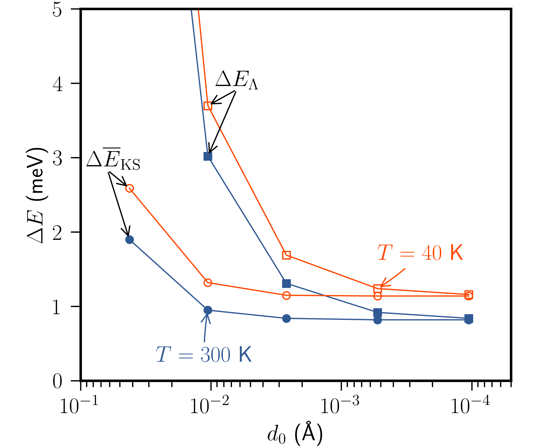
Figure 1: Convergence of $\Delta\overline{E}_{\rm KS}=\overline{E}_{\rm KS}-\overline{E}^{\rm BO}_{\rm KS}$ and $\Delta\overline{E}_{\Lambda}=E_{\Lambda}-\overline{E}^{\rm BO}_{\rm KS}$ with respect to sub-stepping parameter $d_{0}$. Averaging is performed over the beads (including sub-beads). Note, these curves do not represent simulation averages, but rather energies corresponding to one particular ring configuration randomly drawn from the MD simulation for the corresponding temperature.

III.2 Path Integral Monte Carlo

We implemented the PIMC algorithm that uses staging coordinatesTuckerman et al. (1993); Tuckerman (2010), as reviewed in Appendix A. The electronic part is treated with it-TDDFT method presented here (denoted as it-PIMC below) or Born-Oppenheimer DFT (denoted BO-PIMC). Any average can be obtained by using Eq.s (24),(27). For the average energy, it is convenient to use the following thermodynamic relation:

$$E = -\frac{\partial}{\partial\beta}\ln{Z}=$$ (35)

$$= \lim_{K\rightarrow\infty}\left<\frac{KD}{2\beta}-\sum_{j=1}^{K}\left\{\sum_{I=1}^{N_{\rm ion}}\frac{KM_{I}}{2\hbar^{2}\beta^{2}}\left(\vec{R}_{I}^{(j)}-\vec{R}_{I}^{(j+1)}\right)^{2}\right\}+{\overline{E}}_{\rm KS}\right>,$$

where the average is taken over appropriately distributed configurations $\{\vec{R}\}$ and $D$ is the dimensionality of the system. The last term inside angular brackets is obtained with the help of the Hellmann-Feynman theorem (see Appendix C). Because for low temperatures the number of time slices required is large ($>200$), some degree of parallel processing is needed even for small systems. For Born-Oppenheimer PIMC and PIMD algorithms, parallelism is trivial due to the independence of the electronic systems at each bead. In the present method the electronic systems at different beads are not independent. To deal with this problem we first run a long BO constant-temperature PIMD simulation, in order to generate independent starting configurations. By drawing from this set of configurations, a suitable number of non-adiabatic PIMC simulations can then be started in parallel.

IV Results

We report results of physical properties of some prototypical systems using our method. We simulated the H₂ molecule at $T=40$ K and $T=300$ K using the PIMC method, with $K=381$ and $K=50$ beads, respectively, and using $d_{0}=0.0026$ Å ($0.005$ Bohr) in both cases. We found that less than 1000 of accepted MC steps are sufficient for equilibration after sufficiently long thermalization with staging-coordinate BO-PIMD ($\sim 1.5\cdot 10^{5}$ steps with 0.05 fs time steps). In all cases, we started averaging after 1000 MC steps. We used the triple-$\zeta$ plus triple-$\zeta$ polarization shell (TZTP) basis set and the local density approximation (LDA) with the Ceperley-Alder (CA) exchange-correlation functionalCeperley and Alder (1980) and a standard pseudopotential from the SIESTA database. Local and semi-local exchange-correlation functionals such as CA have large self-interaction error in case of $H_{2}$ molecule Johnson et al. (1994). However we emphasize that the goal of the simulations here is to compare our method to the standard approaches and not to the experimental data (for recent high accuracy experimental measurements of H₂ molecule see Refs. Dickenson et al. (2013); Cheng et al. (2018) and references there in). For this purpose our choices of exchange-correlation functional and pseudopotential are quite adequate. We use the same DFT parameters in all calculations to facilitate this comparison. The bond length we obtained after the standard relaxation with the settings and functional described above is 0.78 Å. In both BO-PIMC and it-PIMC we obtained about the same bond length of $\sim$0.81 Å for both temperatures (the experimental bond length for H₂ is 0.74 Å). Although the classical-nuclei bond length is off by  0.04 Å (as expected for the local functionalJohnson et al. (1994)), 0.030 Å path-integral correction to it is in a reasonable agreement with 0.025 Å  correction obtained in high accuracy calculations Sims and Hagstrom (2006); Bubin and Adamowicz (2003).

The results for the zero-point-energy (ZPE) obtained with different methods are summarized in Table 1. First we calculate the ZPE using standard Born-Oppenheimer harmonic approximation, with vibrational frequency corresponding to the DFT potential for the H₂ molecule. The harmonic approximation overestimates the ZPE because the high ZPM of the molecule explores the anharmonic region of the potential. The energy at $T=40$ K calculated with the Morse potential (with parameters fitted to match the interatomic potential obtained in our DFT computations) agrees well with that obtained from BO-PIMC simulations after taking into account the rotational and thermal motion using standard rigid rotor and ideal gas partition functions. However, these methods underestimate the ZPE by $\sim 10$ meV in comparison to our exact imaginary-time PIMC (it-PIMC) results. This correction to BOA agrees well to $14.1$ meV obtained previously in highly accurate analytic-variational and quantum Monte Carlo calculations of H₂ molecule Wolniewicz (1995, 1993); Chen and Anderson (1995); Tubman et al. (2014). Approximately the same difference is observed between BO-PIMC and it-PIMC at $T=300$ K, which is not surprising due to the high frequency of the H₂ molecule vibration. This agreement with the exact calculation is quite good in comparison to $\sim$160 meV obtained in multi-component DFT computationsKreibich et al. (2008). Thus our method can also be used to aide the design of multi-computations density functionals because both methods can be set to share the same electronic parts of the functional. Energy differences between BOA and it-TDDFT in Fig. 1 (see also Table 2) and in Table 1 differ by one order of magnitude. This is because in Fig. 1 the difference is between two methods applied to the same ring polymer and the electronic energy only, while in Table 1 the differences of the total energy are averaged over a large number of configurations. In fact, after decomposing the energy expression of Eq. (35) into nuclear kinetic and electronic parts we observed that the difference is mostly due to the nuclear kinetic energy part. This can be explained by the following. At a given temperature within the BO-PIMC the nuclear kinetic energy and the electronic energy are partitioned in a certain fraction. The it-PIMC leads to a repartitioning in which the contribution of the nuclear kinetic energy is higher as compared to its value in the BO case. This is accomplished in the it-PIMC procedure by preferring configurations that have, on average, shorter distances between the beads, which lowers the E_Λ obtained from it-TDDFT. This makes the electronic energy close to the BO electronic ground-state energy.

These results suggest that even for systems like the H₂ molecule which has a wide gap between occupied and unoccupied energy levels, the it-TDDFT correction to the BO approximation is quite significant, being roughly 5% of the ZPE. We expect these corrections to be larger for systems with a smaller bandgap and even more so in metallic phases, as in the hypothesized high-pressure phase of bulk atomic hydrogen.

$T(K)$	$E^{0}_{\rm harm}$	$E^{0}_{\rm Morse}$	$E^{0}_{\rm BO-PIMC}$	$E^{0}_{\rm it-PIMC}$
40	279	228	228.0(2)	237(1)
300	356	312	292(1)	301(1)

Table 1: $E^{0}=E^{\rm ZPE}+E^{\rm rot}+E^{\rm COM}$ calculated with four methods (all values in meV). Here $E^{\rm ZPE}$ stands for vibrational zero-point energy, $E^{\rm rot}$ and $E^{\rm COM}$ are rotational and center-of-mass motion energies at the given temperature, respectively. $E^{0}_{\rm harm}$ is calculated by computing ZPE using the H₂ harmonic frequency (516.8 meV) and adding a rotational (rigid rotor) and the center of mass motion contributions. $E^{0}_{\rm Morse}$ uses the ZPE estimated from a Morse potential fitted to match the DFT potential energy, again taking into account the rotational and center-of-mass motion energy. $E^{0}_{\rm BO-PIMC}$ and $E^{0}_{\rm it-PIMC}$ are the energies computed from BO-PIMC and exact it-PIMC simulations, respectively. For MC simulations one standard deviation uncertainty is indicated in parentheses.

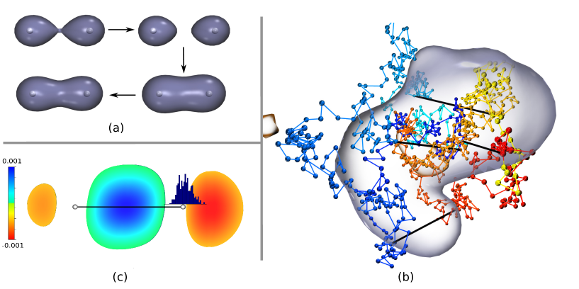
Figure 2: (a) The electron density evolution along the first four beads of the ring-polymer representing the H₂ molecule ($T=40$ K). (b) Atomic positions and average density difference between the present method and the BO approximation for the ring-polymer representing H₂. Black lines depict the bond between two atoms on the time slice (shown for intervals of 100 time slices). The bead color corresponds to time slice, with colors varying from red to yellow for the first atom and from blue to cyan for the second. (c) The average density difference (in units of electrons/ų) shown with the molecular axis rotated to be in the same direction for all time-slices by keeping the center of mass of the molecule at the same position and carrying out the average over all time slices. Blue-green and red-orange isosurfaces represents the excess of electron and of hole, respectively. The dark-blue distribution above the right atom represents is the distribution of the distances between two atoms along the ring-polymer in imaginary time.

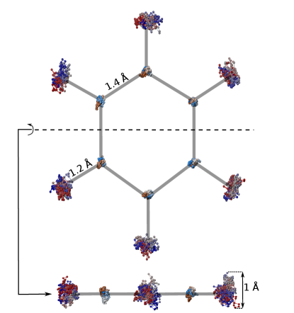
Figure 3: The interacting ring-polymers representing the spacetime positions of the atoms of the benzene molecule at $T=40$ K, top and side views. The solid lines connect the equilibrium positions of each atom. The same color is used to denote that these positions belong to the same imaginary time-slice with lighter colors used for carbon atoms.

In Fig. 2(a) we present the imaginary-time evolution of the electronic density distribution for the first four time-slices for the H₂ molecule. For proper comparison, we rotated the molecular axis to be in the same direction for all time-slices and kept the center of mass of the molecule at the same position. As the distance between the two hydrogen atoms in the molecule fluctuates the electronic density adjusts from one in which the electrons are localized at each atom (when the distance between the atoms is relatively large) to one in which the electrons are shared by the two atoms. We note that the electronic wavefunctions which determine the density are also defined and evaluated at intermediate times between two successive beads. In going from one bead to the next the wavefunction is determined by evolving the wavefunction which corresponds to the first bead by applying the imaginary time evolution operator. The final wavefunction is determined for the entire ring-polymer simultaneously by applying the evolution operator which corresponds to the entire ring several times until we obtain convergence.

In Fig. 2(b) we give an example of a ring-polymer configuration of the imaginary-time positions of the two atoms in the H₂ molecule. The size of the rms deviation of each atom from their equilibrium position is large as compared to the interatomic distance. These atomic position fluctuations are correlated between the two atoms to a significant degree: when one of the atoms moves in a certain direction going from one bead to the next, the other atom is more likely to move in the same direction by a similar amount. In the same plot we also present the averaged difference in the density distribution obtained with our method from that obtained by applying the Born-Oppenheimer approximation, across the space-time configuration in 3D space. In our method, we find an enhancement in the density between atoms compared to the BO approximation result. In Fig. 2(c) we present the same difference in the density distribution, after rotating and shifting the molecule so that its center of mass is fixed and the bond is on the $x$-axis. The asymmetry in the electronic density in Fig. 2(c) is due to the fact that the average is done over a single path in which the center of mass is moving in imaginary time and that implies each atom moves by different amount and not necessarily in opposite directions. This has important implications that we discuss below.

In Fig. 3 we show the ring-polymers that represent the space-time configuration of the carbon and hydrogen atoms in the benzene molecule. As expected, the positions of the hydrogen atoms have large fluctuation, while the heavier carbon atoms have much smaller position fluctuations within the ring-polymer.

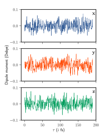
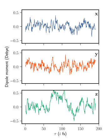
Figure 4: Imaginary-time evolution of the dipole moment along a single path for (a) the H₂ molecule and (b) the benzene molecule.

Due to the imaginary-time propagation of the electronic degrees of freedom the mirror symmetry of electronic density is broken. This asymmetry implies a fluctuation of dipole moment along a single path, which is shown in Fig. 4 for the H₂ and the benzene molecules. The symmetry is restored after summation over all paths in the case of an isolated molecule. When more than one molecule is present the fluctuation of the molecular dipole moment can lead to van der Waals forces between molecules. In our imaginary-time path-integral method the presence of van der Waals forces will be manifested by increased contribution of the ring-polymer configurations where the molecular dipole moments are correlated to produce attraction. This asymmetry is not present within the BO approximation because the wavefunctions at each bead correspond to the ground state density distribution for each bead configuration. In our case, however, we consider the imaginary-time DFT evolution starting from each bead configuration until we reach the next, and our wavefunction is an eigenstate of the entire polymer-ring configuration.

V Discussion and conclusions

We have developed an ab initio method to extend the DFT approach to include the ionic zero-point motion exactly. We employ the usual Feynman path-integral approach where the atomic coordinates form ring-polymers in which each bead represents the atomic positions at different imaginary-time slices. The main idea is that we can actually propagate exactly within DFT the electronic degrees of freedom along each ring-polymer and this allows us to define a space-time DFT super-wavefunction and electronic density which characterizes the entire ring-polymer. This includes imaginary-time correlations of the electronic state between different beads of the ring-polymer. This exact propagation effectively incorporates the effect of all virtual electronic states without limiting the description of the system to the usually adopted BO approximation.

As test cases, we applied our method to the H₂ molecule and the benzene molecule. We find that the difference between our “exact” treatment and the BO approximation is non-negligible when the system contains light atoms, like hydrogen. This energy difference will be significant when ionic zero-point motion plays an important role in determining the prevalent ordered state, like occurrence of charge density waves. Another obvious example of relevance is the case of highly pressurized hydrogenMcMahon et al. (2012); Dias and Silvera (2017), where the zero-point motion is expected to play a significant role, not only in determining the transition temperature and pressure but, more importantly, in determining which of the competing phases prevails in the various regimes of the phase diagram. We also expect our method to be useful in understanding the behavior of systems that involve hydrogen bonding and proton exchange, which are common in water and in various organic and biological molecules. While in general our method requires the entire spectrum of the electronic system, in systems in which the electronic ground state is separated from the first excited state by a gap $\Delta$, our method provides information for all $k_{B}T\ll\Delta$. Even in the case where in the electronic system the difference between the ground state and the first excited state is as small as, say, $\Delta\sim$ 0.3 eV, our approach should be reliable at as high as room temperature.

Furthermore, the present accurate approach can find application in several other systems in condensed matter physics where the effects of correlated motion between electrons and ions is suspected to play an important role. Examples include those where there is a Pierls instability where its formation is assisted by a correlated electron-ion motion, the recently discovered superconductivity in hydratesDrozdov et al. (2015), as well as various polaronic problems. It is also possible such an approach to find application in astrophysics, for example, in studies of superconductivity in very cold brown-dwarf stars (assuming that cold brown-dwarfs exist) where the electron and ions should be moving in a correlated fashion.

Appendix

V.1 Path integral Monte Carlo

In our implementation of PIMC we use the following transformation to staging coordinates as defined in previous workPollock and Ceperley (1984); Tuckerman (2010); Tuckerman et al. (1993):

$$\vec{u}^{(j+k)}=\vec{R}^{(j+W)}-\frac{k\vec{R}^{(j+k+1)}-\vec{R}^{(j)}}{k+1},\;\;k=1,2,\ldots,W,$$ (36)

where $W$ is the segment length (algorithm parameter) and $j$ is a randomly chosen bead. The corresponding terms in ${\cal S}_{E}$ (Eq. (13)) transform as:

$$\sum_{I=1}^{N_{\rm ion}}\sum_{k=0}^{W}\frac{M_{I}}{2\hbar^{2}\Delta\tau}\left|\vec{R}^{(j+k+1)}_{I}-\vec{R}^{(j+k)}_{I}\right|^{2}=$$

$$\sum_{I=1}^{N_{\rm ion}}\frac{M_{I}}{2\hbar^{2}\Delta\tau}\left[\sum_{k=1}^{W}\frac{k+1}{k}\left|\vec{u}^{(j+k)}_{I}\right|^{2}+\frac{1}{W+1}\left|\vec{R}^{(j+W+1)}_{I}-\vec{R}^{(j)}_{I}\right|^{2}\right]$$ (37)

This PIMC algorithm employs two types of moves: (i) randomly choosing bead $j$ and drawing new coordinates from the Gaussian distribution for the transformed coordinates $\vec{u}$ and (ii) random displacement $\vec{s}$ of the whole ring. The move is accepted or rejected depending on the ratio of current (c) and proposed (p) $\Lambda_{\rm max}$ : if $q=\Lambda_{\rm max}^{p}/\Lambda_{\rm max}^{c}={\rm e}^{-\beta(E^{p}_{\Lambda}-E^{c}_{\Lambda})}\geq 1$ the move is accepted, otherwise it is accepted if $r<q$, with $r$ being a uniform random number in the $[0,1)$ interval. $W$ and $s$ are chosen so that the acceptance rate is around 40%.

V.2 Path integral molecular dynamics

For the molecular dynamics sampling method the staging coordinates are defined by the following relationTuckerman (2010); Tuckerman et al. (1993):

$$\vec{u}^{(1)} = \vec{R}^{(1)}$$

$$\vec{u}^{(j)} = \vec{R}^{(j)}-\frac{(j-1)\vec{R}^{(j+1)}+\vec{R}^{(1)}}{j},\;j=2,...,K.$$ (38)

Then the partition function, which yields the same averages as the one in Eq. (25), can be constructed as:

$$Z = {\rm e}^{-\beta{\cal H}_{\rm cl}},$$ (39)

$${\cal H}_{\rm cl} \equiv \sum_{j=1}^{K}\sum_{I=1}^{N_{\rm ion}}\left(\frac{[\vec{P}_{I}^{(j)}]^{2}}{2{\bar{M}}_{I}^{(j)}}+\frac{1}{2}M_{I}^{(j)}\omega_{K}^{2}u^{(j)^{2}}\right)$$ (40)

$$+ E_{\Lambda}(\{\vec{R}\}),$$

$$M_{I}^{(1)} = 0,\ M_{I}^{(j)}=\frac{j}{j-1}M_{I}\ (j>1),$$ (41)

$${\bar{M}}^{(1)}_{I} = M_{I},\ {\bar{M}}^{(j)}_{I}=M_{I}^{(j)}\ (j>1),$$ (42)

$$\omega_{K} = \frac{\sqrt{K}}{\beta\hbar}.$$ (43)

${\cal H}_{\rm cl}$ in Eq. (40) is a classical Hamiltonian with fictitious momenta $\vec{P}_{I}^{(j)}$ associated with each bead. The forces on the beads are derived in the Appendix Section C. $Z$ can the be sampled from a standard MD simulation. To keep the temperature constant we couple every ionic degree of freedom in the system to Nosé-Hoover chain or Langevin thermostat.

V.3 Hellman-Feynman theorem for the ring-polymer

In order to derive Eq.(35) we need to evaluate the derivative of $\Lambda_{\rm max}$ with respect to $\beta$:

$$\frac{\partial}{\partial\beta}\Lambda_{\rm max}=\frac{\partial}{\partial\beta}\langle\mathbf{\Psi}^{(K)}_{0}|\hat{\mathbf{T}}|\mathbf{\Psi}^{(K)}_{0}\rangle$$ (44)

Because $\mathbf{\Psi}^{(K)}_{0}$ is the self-consistent eigenvector of $\hat{\mathbf{T}}$,

$$\frac{\partial}{\partial\beta}\Lambda_{\rm max}=\langle\mathbf{\Psi}^{(K)}_{0}|\frac{\partial}{\partial\beta}\hat{\mathbf{T}}|\mathbf{\Psi}^{(K)}_{0}\rangle$$ (45)

Then

$$\frac{\partial}{\partial\beta}\hat{\mathbf{T}}=\frac{\partial}{\partial\beta}\prod_{j}\hat{T}^{(j)}=\sum_{j}\hat{T}^{(1)}\ldots\hat{T}^{(j-1)}\frac{\partial\hat{T}^{(j)}}{\partial\beta}\hat{T}^{(j+1)}\ldots\hat{T}^{(K)}$$

$$=-\frac{1}{K}\sum_{j}\hat{T}^{(1)}\ldots\hat{T}^{(j-1)}\cdot\hat{\cal H}_{\{\vec{R}^{(j)}\}}[n(j\Delta\tau)]\cdot\hat{T}^{(j)}\ldots\hat{T}^{(K)}$$ (46)

The last equality is derived by writing $\hat{T}^{(j)}$ directly as the iterative solution of the it-TDDFT Eq. (4) and taking into account the fact that $\Lambda_{\rm max}$ is stationary with respect to variation of $\mathbf{\Psi}^{(K)}_{0}$, therefore terms containing $\int d\vec{r}\ \delta{\cal H}_{\{\vec{R}^{(j)}\}}/\delta n(\vec{r},j\Delta\tau)\cdot\partial n(\vec{r},j\Delta\tau)/\partial\beta$ vanish. Then,

$$\langle\mathbf{\Psi}^{(K)}_{0}|-\frac{1}{K}\sum_{j}\hat{T}^{(1)}\ldots\hat{T}^{(j-1)}\cdot{\cal H}_{\{\vec{R}^{(j)}\}}[n(j\Delta\tau)]\cdot\hat{T}^{(j)}\ldots\hat{T}_{K}|\mathbf{\Psi}^{(K)}_{0}\rangle$$

$$=-\frac{1}{K}\sum_{j}\lambda^{(1)}\ldots\lambda^{(j-1)}\langle\Psi^{(j)}|{\cal H}_{\{\vec{R}^{(j)}\}}[n(j\Delta\tau)]|\Psi^{(j)}\rangle\lambda^{(j)}\ldots\lambda^{(K)}$$

$$=-\frac{\Lambda_{\rm max}}{K}\sum_{j}E^{(j)}_{\rm KS},$$ (47)

where $\lambda^{(j)}$ is defined by $\lambda^{(j)}|\Psi^{(j)}\rangle=\hat{T}^{(j)}|\Psi^{(j+1)}\rangle$, with $\Psi^{(j)}$ being the normalized electronic wavefunction corresponding to $\mathbf{\Psi}^{(K)}_{0}$ at the time-slice $j$, see also Eq.s (31)-(32). Eq. (47) leads to Eq. (35) in the main text.

Similarly, $\vec{F}_{\rm ele}^{(j)}$, the electronic component of the total force on the bead $j$, required for the molecular dynamics sampling algorithm can be derived from

$$\vec{F}^{(j)}_{\rm ele}=-\nabla_{\vec{R}^{(j)}}E_{\Lambda}=\frac{1}{\beta}\nabla_{\vec{R}^{(j)}}\ln\Lambda_{\rm max}=\frac{1}{\Lambda_{\rm max}\beta}\nabla_{\vec{R}^{(j)}}\Lambda_{\rm max}$$ (48)

Following the same steps as for Eqs. (44–47) we get

$$\vec{F}^{(j)}_{\rm ele}=-\frac{1}{K}\nabla_{\vec{R}^{(j)}}E^{(j)}_{\rm KS}$$ (49)

V.4 Convergence of $\Delta\overline{E}_{\rm KS}$ and $\Delta E_{\Lambda}$

For a more quantitative comparison of convergence rates, we provide here the values of the quantities $\Delta\overline{E}_{\rm KS}$ and $\Delta E_{\Lambda}$, as well as the actual value of the average $\overline{E}_{\rm KS}^{\rm BO}$, for different values of the sub-stepping parameter $d_{0}$.

$d_{0}$,Bohr	H2, $T=300$ K, $K=36$			H2, $T=40$ K, $K=381$
	$\Delta\overline{E}_{\rm KS}$	$\Delta E_{\Lambda}$	$\overline{E}_{\rm KS}^{\rm BO}$	$\Delta\overline{E}_{\rm KS}$	$\Delta E_{\Lambda}$	$\overline{E}_{\rm KS}^{\rm BO}$
0.08	$1.90$	$12.33$	-30457.66	2.59	14.32	-30519.72
0.02	$0.95$	$3.02$	-30456.94	1.32	3.70	-30520.02
0.005	$0.84$	$1.31$	-30457.93	1.15	1.69	-30520.12
0.001	$0.82$	$0.92$	-30458.19	1.14	1.24	-30520.09
0.0002	$0.82$	$0.84$	-30458.24	1.14	1.16	-30520.09

Table 2: The data for Fig. 1. Energies are in meV and $d_{0}$ is given in units of the Bohr radius. Averaging is done over the beads (including sub-beads) for a single ring-polymer configuration (see Fig. 2) .

References

- Payne et al. (1992) M. C. Payne, M. P. Teter, D. C. Allan, T. A. Arias, and J. D. Joannopoulos, Rev. Mod. Phys. 64, 1045 (1992).
- Marx and Hutter (2009) D. Marx and J. Hutter, Cambridge University Press, Cambridge, England (2009).
- Ceperley (1995a) D. M. Ceperley, Rev. Mod. Phys. 67, 279 (1995a).
- Pierce and Manousakis (1998) M. Pierce and E. Manousakis, Phys. Rev. Lett. 81, 156 (1998).
- Pierce and Manousakis (1999a) M. Pierce and E. Manousakis, Phys. Rev. B 59, 3802 (1999a).
- Pierce and Manousakis (1999b) M. E. Pierce and E. Manousakis, Phys. Rev. Lett. 83, 5314 (1999b).
- Pierce and Manousakis (2000) M. E. Pierce and E. Manousakis, Phys. Rev. B 62, 5228 (2000).
- Ceperley and Manousakis (2001) D. M. Ceperley and E. Manousakis, J. Chem. Phys. 115, 10111 (2001).
- Pollock and Ceperley (1984) E. L. Pollock and D. M. Ceperley, Phys. Rev. B 30, 2555 (1984).
- Ramírez and Herrero (1993) R. Ramírez and C. P. Herrero, Phys. Rev. B 48, 14659 (1993).
- Kaxiras and Guo (1994) E. Kaxiras and Z. Guo, Phys. Rev. B 49, 11822 (1994).
- Noya et al. (1996) J. C. Noya, C. P. Herrero, and R. Ramírez, Phys. Rev. B 53, 9869 (1996).
- Herrero and Ramirez (2014) C. P. Herrero and R. Ramirez, J. Phys.: Condens. Matter 26, 233201 (2014).
- Ramírez et al. (2006) R. Ramírez, C. P. Herrero, and E. R. Hernández, Phys. Rev. B 73, 245202 (2006).
- McMahon et al. (2012) J. M. McMahon, M. A. Morales, C. Pierleoni, and D. M. Ceperley, Rev. Mod. Phys. 84, 1607 (2012).
- Pisana et al. (2007) S. Pisana, M. Lazzeri, C. Casiraghi, K. S. Novoselov, A. K. Geim, A. C. Ferrari, and F. Mauri, Nat. Mater. 6, 198 (2007).
- Vidal-Valat et al. (1992) G. Vidal-Valat, J.-P. Vidal, K. Kurki-Suonio, and R. Kurki-Suonio, Acta Crystallogr. Sect. A 48, 46 (1992).
- Bunker (1977) P. R. Bunker, Journal of Molecular Spectroscopy 68, 367 (1977).
- Coxon and Hajigeorgiou (1991) J. A. Coxon and P. G. Hajigeorgiou, Journal of Molecular Spectroscopy 150, 1 (1991).
- Schwenke (2001) D. W. Schwenke, J. Phys. Chem. A 105, 2352 (2001).
- Tubman et al. (2014) N. M. Tubman, I. Kylänpää, S. Hammes-Schiffer, and D. M. Ceperley, Phys. Rev. A: At., Mol., Opt. Phys. 90, 042507 (2014).
- Mitroy et al. (2013) J. Mitroy, S. Bubin, W. Horiuchi, Y. Suzuki, L. Adamowicz, W. Cencek, K. Szalewicz, J. Komasa, D. Blume, and K. Varga, Rev. Mod. Phys. 85, 693 (2013).
- Wolniewicz (1995) L. Wolniewicz, J. Chem. Phys. 103, 1792 (1995).
- Wolniewicz (1993) L. Wolniewicz, J. Chem. Phys. 99, 1851 (1993).
- Chen and Anderson (1995) B. Chen and J. B. Anderson, J. Chem. Phys. 102, 2802 (1995).
- Yang et al. (2015) Y. Yang, I. Kylänpää, N. M. Tubman, J. T. Krogel, S. Hammes-Schiffer, and D. M. Ceperley, J. Chem. Phys. 143, 124308 (2015).
- Webb et al. (2002) S. P. Webb, T. Iordanov, and S. Hammes-Schiffer, J. Chem. Phys. 117, 4106 (2002).
- Chakraborty et al. (2008) A. Chakraborty, M. V. Pak, and S. Hammes-Schiffer, J. Chem. Phys. 129, 014101 (2008).
- Kylänpää and Rantala (2010) I. Kylänpää and T. T. Rantala, J. Chem. Phys. 133, 044312 (2010).
- Kohn and Sham (1965) W. Kohn and L. J. Sham, Phys. Rev. 140, A1133 (1965).
- Kreibich and Gross (2001) T. Kreibich and E. K. U. Gross, Phys. Rev. Lett. 86, 2984 (2001).
- Kreibich et al. (2008) T. Kreibich, R. van Leeuwen, and E. K. U. Gross, Phys. Rev. A: At., Mol., Opt. Phys. 78, 022501 (2008).
- Lüders et al. (2005) M. Lüders, M. A. L. Marques, N. N. Lathiotakis, A. Floris, G. Profeta, L. Fast, A. Continenza, S. Massidda, and E. K. U. Gross, Phys. Rev. B 72, 024545 (2005).
- Marques et al. (2005) M. A. L. Marques, M. Lüders, N. N. Lathiotakis, G. Profeta, A. Floris, L. Fast, A. Continenza, E. K. U. Gross, and S. Massidda, Phys. Rev. B 72, 024546 (2005).
- Barker (1979) J. Barker, J. Chem. Phys. 70, 2914 (1979).
- Chandler and Wolynes (1981) D. Chandler and P. G. Wolynes, J. Chem. Phys. 74, 4078 (1981).
- Cao and Berne (1993) J. Cao and B. J. Berne, J. Chem. Phys. 99, 2902 (1993).
- Marx and Parrinello (1994) D. Marx and M. Parrinello, Z. Phys. B (Rapid Note) 95, 143 (1994).
- Marx and Parrinello (1996) D. Marx and M. Parrinello, J. Chem. Phys. 104, 4077 (1996).
- Benoit et al. (1998) M. Benoit, D. Marx, and M. Parrinello, Nature 392, 258 (1998).
- Marx et al. (1999) D. Marx, M. E. Tuckerman, J. Hutter, and M. Parrinello, Nature 397, 601 (1999).
- Morrone and Car (2008) J. A. Morrone and R. Car, Phys. Rev. Lett. 101, 017801 (2008).
- Städele and Martin (2000) M. Städele and R. M. Martin, Phys. Rev. Lett. 84, 6070 (2000).
- Johnson and Ashcroft (2000) K. A. Johnson and N. Ashcroft, Nature 403, 632 (2000).
- Miller III and Manolopoulos (2005) T. F. Miller III and D. E. Manolopoulos, J. Chem. Phys. 123, 154504 (2005).
- Ceriotti et al. (2016) M. Ceriotti, W. Fang, P. G. Kusalik, R. H. McKenzie, A. Michaelides, M. A. Morales, and T. E. Markland, Chem. Rev. 116, 7529 (2016), pMID: 27049513.
- Habershon et al. (2013) S. Habershon, D. E. Manolopoulos, T. E. Markland, and T. F. Miller III, Annual review of physical chemistry 64, 387 (2013).
- Chin et al. (2009) S. A. Chin, S. Janecek, and E. Krotscheck, Chem. Phys. Lett. 470, 342 (2009).
- Mendoza et al. (2014) M. Mendoza, S. Succi, and H. J. Herrmann, Phys. Rev. Lett. 113, 096402 (2014).
- Feynman (1972) R. Feynman, Statistical Mechanics (Addison-Wesley, 1972).
- Feynman et al. (2010) R. Feynman, A. Hibbs, and D. Styer, Quantum Mechanics and Path Integrals, Dover Books on Physics (Dover Publications, 2010).
- Fiolhais et al. (2008) C. Fiolhais, F. Nogueira, and M. Marques, A Primer in Density Functional Theory, Lecture Notes in Physics (Springer Berlin Heidelberg, 2008).
- Giustino (2014) F. Giustino, Materials Modelling Using Density Functional Theory: Properties and Predictions (Oxford University Press, 2014).
- Kolesov et al. (2016) G. Kolesov, O. Grånäs, R. Hoyt, D. Vinichenko, and E. Kaxiras, J. Chem. Theory Comput. 12, 466 (2016).
- Soler et al. (2002) J. M. Soler, E. Artacho, J. D. Gale, A. García, J. Junquera, P. Ordejón, and D. Sánchez-Portal, J. Phys.: Condens. Matter 14, 2745 (2002).
- Castro et al. (2004) A. Castro, M. A. Marques, and A. Rubio, J. Chem. Phys. 121, 3425 (2004).
- Ceperley (1995b) D. M. Ceperley, Rev. Mod. Phys. 67, 279 (1995b).
- Tuckerman et al. (1993) M. E. Tuckerman, B. J. Berne, G. J. Martyna, and M. L. Klein, J. Chem. Phys. 99, 2796 (1993).
- Tuckerman (2010) M. Tuckerman, Statistical mechanics: theory and molecular simulation (Oxford University Press, 2010).
- Ceperley and Alder (1980) D. M. Ceperley and B. J. Alder, Phys. Rev. Lett. 45, 566 (1980).
- Johnson et al. (1994) B. G. Johnson, C. A. Gonzales, P. M. Gill, and J. A. Pople, Chem. Phys. Lett. 221, 100 (1994).
- Dickenson et al. (2013) G. D. Dickenson, M. L. Niu, E. J. Salumbides, J. Komasa, K. S. E. Eikema, K. Pachucki, and W. Ubachs, Phys. Rev. Lett. 110, 193601 (2013).
- Cheng et al. (2018) C.-F. Cheng, J. Hussels, M. Niu, H. L. Bethlem, K. S. E. Eikema, E. J. Salumbides, W. Ubachs, M. Beyer, N. Hölsch, J. A. Agner, F. Merkt, L.-G. Tao, S.-M. Hu, and C. Jungen, Phys. Rev. Lett. 121, 013001 (2018).
- Note (1) More precisely, the average bond lengths were calculated as 0.80995(1) Å and 0.81019(3) Å in it-PIMC at K and K, respectively, and 0.80887(1) Å and 0.80960(1) Å in BO-PIMC calculations at the same values of temperature.
- Sims and Hagstrom (2006) J. S. Sims and S. A. Hagstrom, J. Chem. Phys. 124, 094101 (2006).
- Bubin and Adamowicz (2003) S. Bubin and L. Adamowicz, J. Chem. Phys. 118, 3079 (2003).
- Dias and Silvera (2017) R. P. Dias and I. F. Silvera, Science 17, 715 (2017).
- Drozdov et al. (2015) A. P. Drozdov, M. I. Eremets, I. A. Troyan, V. Ksenofontov, and S. I. Shylin, Nature 525, 73 (2015).