Ray-of-Arrival Passing for Indirect Beam Training in Cooperative Millimeter Wave MIMO Networks

Abstract

This paper is concerned with the channel estimation problem in multi-cell millimeter wave (mmWave) wireless systems. We develop a novel Ray-of-Arrival Passing for In-Direct (RAPID) framework, in which a network consisting of multiple BS are able to work cooperatively to estimate jointly the UE channels. To achieve this aim, we consider the spatial geometry of the mmWave environment and transform conventional angular domain beamforming concepts into the more euclidean, Ray-based domain. Leveraging this model, we then consider the conditional probabilities that pilot signals are received in each direction, given that the deployment of each BS is known to the network. Simulation results show that RAPID is able to improve the average estimation of the network and significantly increase the rate of poorer quality links. Furthermore, we also show that, when a coverage rate threshold is considered, RAPID is able to improve greatly the probability that multiple link options will be available to a user at any given time.

I Introduction

In order to meet the unprecedented throughput demands of next-generation communications systems, mobile networks are expected to become significantly denser in urban areas [1, 2, 3]. By reducing the typical cell size, the number of devices that each base station (BS) needs to support can be decreased; however, the smaller inter-cell spacing can lead to increased interference between cells [4]. Supporting densification, the mmWave frequency range (30 GHz-300 GHz) is an appealing spectrum band, due to its much higher atmospheric losses. This propagation characteristic naturally attenuates inter-cell interference and thus can permit carrier frequencies to be reused in cells in closer proximity to one another [5, 6, 7]. Furthermore, due to its vastly underutilized spectrum, the mmWave frequency range also offers a substantial increase in bandwidth compared to the over-congested microwave spectrum used in existing wireless systems [8, 9]. Although frequency reuse may see a benefit from these propagation losses, the signals also experience significant reflection and penetration losses that together make wireless communication in the mmWave band very challenging [10]. Overcoming these losses is a critical issue that must be resolved, in order for mmWave networks to meet reliability expectations of emerging technologies such as vehicular communications and the industrial Internet-of-Things (IoT) [11, 12].

The most widely accepted means of overcoming mmWave propagation losses is to employ large multiple-input multiple-output (MIMO) antenna arrays with directional beamforming [13, 8, 14]. Beamforming is also advantageous in further reducing interference in small cell networks, as a coordinated approach in this regard can minimize unwanted signals [4, 15]. Moreover, as spacing between antenna array elements is typically proportional to the carrier wavelength, large mmWave antenna arrays can be implemented while occupying a much smaller form factor. However, the much larger bandwidth expectation in an mmWave system also indicates that conventional digital MIMO architectures may have an unrealistic power consumption, due to the large number of high-rate Analog-to-Digital Converters (ADCs) and digital-to-analog converters (DACs).

Even for completely digital systems, estimating large MIMO channel matrices can be a challenging problem. At mmWave frequencies, this becomes more difficult, due to both hardware constraints and the necessity to use beamforming to overcome propagation losses during initial access and channel estimation. On the other hand, due to these propagation losses, measurements have shown that the mmWave channel is sparse in the spatial domain [8]. Leveraging this phenomenon, each channel can be decomposed into its underlying physical parameters, including an angle-of-arrival (AoA), an angle-of-departure (AoD), and a path coefficient, for a small number of propagation paths. Conversely, microwave frequency MIMO channels exhibit rich scattering environments, which leads to channel models that characterize the superposition of many paths. To capture mmWave sparsity, an alternative MIMO matrix representation, known as the “virtual channel matrix,” can be formed from the set of channel gains between each beamforming direction [16, 17]. Thanks to its sparsity, it is often advantageous to estimate this matrix directly by using compressed sensing (CS) techniques to reduce the number of required measurements [18, 19].

An intuitive benchmark approach to estimating the virtual channel matrix involves exhaustively searching the channel for all possible propagation paths. This may be achieved by transmitting and receiving pilot signals while sequentially adopting combinations of beamforming vectors between the transceiver to search for any paths. Improving on this point, hierarchical codebook-based estimation strategies have been proposed, in order to reduce significantly estimation overheads by applying a divide-and-conquer type of beam search [18, 19, 20, 21, 22, 23]. However, as progressive beam refinement converges toward a single path in each estimation process, these approaches have an overhead that is proportional to the number of users and paths. For this reason, approaches that do not adapt toward a specific user, such as Exhaustive Search (ES) and random directional beamforming (RDB), are more appropriate, as they can support the estimation of multiple user channels in the same period [24, 25, 26]. Furthermore, in order to realize a robust and reliable network, it may also be important for each user to maintain multiple link options to the network [27, 28, 29]. In particular, this multi-connectivity would be a crucial form of redundancy to support beam switching when one path direction suddenly becomes blocked. Fortunately, in the ultra-dense, user-centric cells expected in next-generation mobile systems, it follows that each user equipment (UE) will typically be in the coverage of large numbers of BS in a given communication period. Furthermore, due to the close relationship between the environment and the physical parameters that make up the mmWave channel, we are able to infer path directions from the network’s spatial geometry.

For a sparse mmWave channel within dense multi-BS deployments, channels between each UE and BS can exhibit high spatial correlation. As these channels can be expressed directly as a function of the physical environment and array orientations, channel decompositions for multiple BS may have propagation paths that correspond to a common scatterer, or direct line-of-sight (LOS) paths to the same UE. Leveraging the same duality between localization and estimation, joint strategies have been proposed for microwave systems in [30, 31, 32]. Extending these concepts to mmWave systems, [33] proposed a user cooperation estimation strategy which also able to support non-line-of-sight (NLOS) estimation. Although these strategies show a significant improvement over conventional estimations, they often require a precise time difference of arrival (TDoA) or phase information, and they neglect many of the hardware constraints such as hybrid beamforming and quantized phase shifters. Furthermore, as uniform linear arrays (ULAs) are typically considered in mmWave systems, the array orientation is a commonly overlooked variable. In particular, the use of ULAs results in an angle ambiguity problem, where “forward” beamforming pilots/measurements are indistinguishable from the rearward directions (See [24] and Figure 4 therein).

Motivated by the strict hardware constraints in mmWave systems and the need to meet network reliability requirements, we aim to develop a joint channel estimation strategy that is able to utilize spatial dependencies among multiple BS, in order to assist the network’s estimation to each UE. Specifically, in the uplink, we consider a UE that broadcasts beamformed pilot signals which can be jointly received by multiple BS. We also show that, if each BS knows the relative position of its neighbors, this physical deployment information can be utilized to identify conditional geometric relationships that exist between virtual channel estimates. To facilitate this aim, we leverage ray tracing principals to transform the channel AoD/AoA measurements into a more Euclidean-focused ray-of-arrival (RoA) and ray-of-reparture (RoD). We then show that a given pair of RoA measurements, received from two different positions, can be considered to sample jointly a position in Euclidean space. Similarly, we leverage geometric dependencies among the RoD to infer conditional transmit directions. We refer to the developed scheme as “Ray-of-Arrival Passing for In-Direct (RAPID)beam training.”

In contrast to the existing work, by focusing on the virtual channel information, we are able to apply our approach to hardware constrained estimation. Furthermore, to provide generality and reduce computational redundancy, we also consider that each BS is only able to share entries from its already estimated channel. As this matrix is inherently sparse, this greatly reduces the bandwidth required to share information among the network. Furthermore, by considering the virtual channel estimate, RAPID is agnostic to how each independent estimation is carried out, and therefore can be implemented on top of existing channel estimation strategies. Results show that the proposed scheme can greatly increase the achievable rate between the transceiver, particularly for links that would have normally been quite poor. By considering a minimum rate requirement, we also show that RAPID is able to significantly increase the coverage probability for having a greater number of available links.

We summarize the main contributions of this as follows:

• We investigate a multi-cell user-centric mmWave communication system, in which a UE broadcasts pilot signals to a number of BSs. We generalize the concept of the AoD/AoA beamforming to a ray-based RoD/RoA estimation. We apply this model to the widely used ULA, and develop an estimator that is robust to the angle ambiguity problem. We also show that for a BS pair with a known relative displacement, many of their virtual channel entries are mutually dependent.

• We use the Ray-based model to develop a Bayesian estimator so that each BS may compute the probability of a path on its beamforming directions, given the channel estimates provided by the other network BSs. Results show a significant improvement for both the average achievable rate and network coverage when compared to conventional schemes.

• In order to reduce sharing overheads in bandwidth constrained networks, we exploit the channel sparsity and propose to use limited information exchange among BS. To this end, we reduce the interchange to only the most dominant virtual channel entries, that exhibit a mutually dependent relationship for another BS. In addition to this, we also show that the only prior information required for RAPID is the relative position and orientation of each BS. In this sense, if the UE is also aware of this relative deployment, the proposed scheme can also be applied to the downlink. By adopting multiple access scheme for downlink pilots such as Code Division Multiple Access (CDMA), no sharing overhead would be required in this case.

II System Model

Consider a mmWave cellular network consisting of $B$ BS—each equipped with an array of $N_{\!B\!S}$ antenna. We adopt a user-centric deployment model, in which a UE is located at the origin of a two-dimensional coordinate system (i.e., $(x_{u},y_{u})=(0,0)$). We further assume that the UE is equipped with an array of $N_{\!U\!E}$ antennas. Relative to the origin of this system, we consider that the deployment of the $b$th BS antenna array can be described by a 2D translation and a rotation, denoted by $\bm{D}_{b}=(x_{b},y_{b})$ and $\Theta_{b}$, respectively. We consider both the BS and UE antenna arrays to have an orientation denoted by $\Theta_{b}\in[-\pi,\pi]$ and $\psi_{u}\in[-\pi,\pi]$, respectively. We consider this orientation to be defined as the counter-clockwise angle from the x-axis to the ULA. We further denote the relative displacement vector from the $p$th BS to the $q$th BS as $\bm{\Delta}_{p,q}=[\delta_{x_{p,q}},\delta_{y_{p,q}}]=\bm{D}_{p}-\bm{D}_{q}$ . In this paper, we use the term “local reference frame” to refer to angles relative to a particular antenna array. Conversely, angles in the “global reference frame” refer to absolute angles in the global 2D coordinate system. This distinction is important, as UE orientation cannot be known to the network a priori. An example deployment configuration is shown in Fig. 1.

To estimate the uplink channel matrix, we assume that each UE simultaneously broadcasts a sequence of beamformed pilot signals. Similarly, all BS collect these signals by adopting a sequence of beamforming vectors. We consider that both the UE and each BS are equipped with a limited number of radio frequency (RF) chains, denoted by $R_{\!B\!S}$ and $R_{\!U\!E}$, respectively. Denote $\bm{f}_{i}$ as the $N_{\!U\!E}\times 1$ transmit beamforming vector adopted by the $i$th RF chain at the UE. Similarly, denote by $\bm{w}_{j}^{(b)}$, the $N_{\!B\!S}\times 1$ receiving beamforming vector adopted by the $j$th RF chain of the $b$th BS.

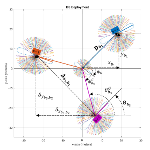
Figure 1: An example deployment illustrating each parameter in our model. The UE can be seen at the origin, with antenna array orientation denoted by $\psi_{u}$. Similarly, each BS is deployed at $bm{D}_{b}=(x_{b},y_{b})$ and with orientation $\Theta_{b}$. To make the illustration more explicit, we show $B=3$ BS, indexed as $b_{1}=1$, $b_{2}=2$ and $b_{3}=3$. Relating to the Euclidean channel model, we label the angle-of-departure (AoD)in the UE local reference frame (i.e., relative to its own array orientation) “$\phi^{L}_{b}$” and the corresponding global reference frame (i.e., relative to the global coordinate system) angle “$\phi^{G}_{b}$.” Similarly for each BS, we have the local reference frame angle-of-arrival (AoA)as $\theta^{L}_{b}$ and the global angle as $\theta^{G}_{b}$.)

Following [18], we consider the beamforming vectors, at each link end, as being limited to networks of RF phase shifters. As such, all elements of $\bm{f}_{i}$ and $\bm{w}_{i}^{(b)}$ are constrained to have a constant modulus and unit norm, such that $||\bm{f}_{i}||=1,\forall$ $i=1,\cdots,R_{\!U\!E}$, and $||\bm{w}_{j}^{(b)}||=1,\forall$ $j=1,\cdots,R_{\!B\!S},b=1,\cdots,B$. We further assume that due to hardware constraints, each of the phase shifters (i.e., the entries of $\bm{f}_{i}$ and $\bm{w}_{j}^{(b)}$ ) is digitally controlled and takes on quantized values from the predetermined set

$$\left\{\frac{1}{\sqrt{N}}\text{exp}(jq_{k})\right\},\forall k=1,\cdots,N,$$ (1)

where $q_{k}=\pi-2\pi(k-1)/N$ and $N\in\{N_{\!U\!E},N_{\!B\!S}\}$ is the number of antennas in the array. That is, each UE (BS) phase shifter can only use one $N_{\!U\!E}$ ($N_{\!B\!S}$) uniformly spaced point around the unit circle, respectively, which can therefore be digitally controlled by $\lceil\text{log}_{2}N\rceil$ bits.

Let $\bm{F}=[\bm{f}_{1},\bm{f}_{2},\cdots,\bm{f}_{R_{\!U\!E}}]$ denote the $N_{\!U\!E}\times R_{\!U\!E}$ UE beamforming matrix, with columns representing the $R_{\!U\!E}$ RF beamforming vectors. The corresponding $N_{\!U\!E}\times 1$ UE transmit signal can be represented as

$$\bm{x}=\sqrt{\frac{P}{R_{\!U\!E}}}\bm{F}\bm{s},$$ (2)

where $P$ is the UE’s pilot transmit power and $\bm{s}$ is the ${R}_{\!B\!S}\times 1$ vector of transmit pilot symbols corresponding to each beamforming vector with $E[\bm{s}\bm{s}^{H}]=\bm{I}_{R_{\!U\!E}}$. We adopt the widely used block-fading channel model, such that the signal observed by the $b$th BS can be expressed as [26]

$$\bm{r}^{(b)} =\bm{H}^{(b)}\bm{x}+\bm{q}^{(b)}=\sqrt{\frac{P}{R_{\!U\!E}}}\bm{H}^{(b)}\bm{F}\bm{s}+\bm{q}^{(b)},$$ (3)

where $\bm{H}^{(b)}$ denotes the $N_{\!B\!S}\times N_{\!U\!E}$ MIMO channel matrix between the UE and the $b$th BS, and $\bm{q}^{(b)}$ is an $N_{\!B\!S}\times 1$ complex additive white Gaussian noise (AWGN) vector for the $u$th user, following distribution $\mathcal{C}\mathcal{N}(\bm{0},N_{0}\bm{I}_{N_{\!B\!S}})$.

Each BS processes the received pilot signals with each of the $R_{\!B\!S}$ RF chains. By denoting $\bm{W}^{(b)}=[\bm{w}_{1}^{(b)},\bm{w}_{2}^{(b)},\cdots,\bm{w}_{R_{\!B\!S}}^{(b)}]$ as the $N_{\!B\!S}\times R_{\!B\!S}$ combining the matrix at the $b$th BS, we express the $R_{\!B\!S}\times 1$ vector of the $b$th BS received signals as

$$\bm{y}^{(b)} =(\bm{W}^{(b)})^{H}\bm{H}^{(b)}\bm{x}+\bm{n}^{(b)}$$ (4)

where the noise term follows the distribution

$$\bm{n}^{(b)}=(\bm{W}^{(b)})^{H}\bm{q}^{(b)}\sim\mathcal{C}\mathcal{N}(\bm{0},N_{0}(\bm{W}^{(b)})^{H}\bm{W}^{(b)}).$$ (5)

We follow [34] and adopt a two-dimensional (2D) sparse geometric channel model. We consider that only a single dominant path is present between the UE and each BS, leaving the extension to joint scatterer estimation as a future work. Using this model, each candidate uplink channel between the UE and the $b$th BS can be characterized in its local reference frame by an AoD, $\phi^{L}_{b}$, an AoA, $\theta^{L}_{b}$, and a path coefficient, namely $\alpha_{b}$. The corresponding MIMO channel between the UE and the $b$th BS can be expressed in terms of these physical parameters as

$$\bm{H}^{(b)}=\alpha_{b}\sqrt{N_{\!U\!E}N_{\!B\!S}}\bm{a}_{\!B\!S}(\theta^{L}_{b})(\bm{a}_{U\!E}(\phi^{L}_{b}))^{H}$$ (6)

where $\bm{a}_{\!B\!S}(\theta^{L}_{b})$ and $\bm{a}_{\!U\!E}(\phi^{L}_{b})$ denote the BS and UE arrays’ spatial signatures, respectively. We adopt a flat block fading model and assume that the path coefficient remains unchanged through the entire channel estimation process. We assume that the value of the path coefficient follows the zero mean complex distribution $\alpha_{b}\sim\mathcal{C}\mathcal{N}(0,\sigma_{R}^{2})$, where the expected power, $\sigma_{R}^{2}$, is inversely proportional to the radial displacement between the BS and UE as $\sigma_{R}^{2}=r_{b}^{-\beta}$, and where $r_{b}=||\bm{D}_{b}||_{2}=\sqrt{x_{b}^{2}+y_{b}^{2}}$ is the radial distance and $\beta$ is the path loss exponent.

We consider that the BS and each UE are equipped with ULA. We can then write $\bm{a}_{\!B\!S}(\phi^{L}_{b})=\bm{u}(\phi^{L}_{b},N_{\!U\!E})$ and $\bm{a}_{\!U\!E}(\theta^{L}_{b})=\bm{u}(\theta^{L}_{b},N_{\!B\!S})$, respectively, whereby

$$\bm{u}(\epsilon,N)\triangleq\frac{1}{\sqrt{N}}[1,e^{j\frac{2\pi d\text{cos}(\epsilon)}{\lambda}},\cdots,e^{j\frac{2\pi d(N-1)\text{cos}(\epsilon)}{\lambda}}]^{T}.$$ (7)

In (7), $N\in\{N_{\!U\!E},N_{\!B\!S}\}$ is the number of antenna elements in the array, $\lambda$ denotes the signal wavelength, and $d$ denotes the spacing between antenna elements. With half-wavelength spacing, the distance between antenna elements satisfies $d=\lambda/2$.

To estimate channel information, beamforming vectors are selected from a predetermined set of candidate beamforming vectors at each link end. We denote the candidate beamforming matrices as $\bm{F}_{c}$ and $\bm{W}_{c}$, the columns of which comprise all candidate beamforming vectors at the UE and BS, respectively. For ease of practical implementation, we consider the candidate beams to be subject to quantized phase-shifting constraints, and therefore they represent the set of all possible beamforming vectors that may be used later for data communication. Following (1), this leads to $N_{\!U\!E}$ orthogonal transmitting candidate beams and $N_{\!B\!S}$ orthogonal receiving candidate beams. The $N_{\!B\!S}\times N_{\!U\!E}$ matrix formed by the product of the MIMO channel and these two candidate beamforming matrices is commonly referred to as the “virtual channel matrix” [18], given by

$$\bm{V}^{(b)}=\frac{1}{\sqrt{N_{\!U\!E}N_{\!B\!S}}}(\bm{W}_{c})^{H}\bm{H}^{(b)}\bm{F}_{c}.$$ (8)

We therefore aim to estimate this matrix so that beam pairs that result in strong channel gains can be identified for data communication. The key challenge here is determining how to design a sequence of beamforming vectors in such a way that the channel parameters can be quickly and accurately estimated, leaving more time for data communication and thus achieving a higher throughput.

To facilitate our proposed cooperative channel estimation scheme, we assume that all BS are able to maintain a reliable link between one another and are thus able to share mutually dependent information. Initially, we consider complete information sharing, however we later restrict this to the bandwidth constrained channel by only sharing dependent measurements of significant signal strength. In the following sections, we leverage mutual channel information, in order to develop a cooperative BS framework.

III RAPID Beam Training

In this section, we first extend our channel model to consider the Euclidean deployment scenario. We then introduce the sequence of measurement beamforming vectors adopted in our proposed estimation scheme, and then we extend these into the 2D geometric model. In doing so, we propose a shift from the conventional single-link-oriented AoD and AoA model, to a more Euclidean-focused RoD and RoA model. Subsequent sections then develop a means of jointly computing the probability of each beamforming combination, given the mutually dependent information provided by cooperating BS.

III-A Euclidean Space MIMO Channel

In order to develop our joint estimation strategy, we begin by incorporating the 2D deployment into the angular channel in (6). To this end, we denote the global AoD of the $b$th propagation path as $\phi^{G}_{b}$, i.e., the angle of the propagation from the global frame, irrespective of the UE orientation. Similarly, we denote the global AoA at the BS end as $\phi^{G}_{b}$. Recalling the array orientations $\psi_{u}$ and $\Theta_{b}$, we can relate global angles into the local reference frame AoD and AoA (i.e., the local beam steering directions) as $\phi^{L}_{b}=\phi^{G}_{b}-\psi_{u}$ and $\theta^{L}_{b}=\theta^{G}_{b}-\Theta_{b}$. Substituting these into (6) leads subsequently to a global description of the channel model

$$\bm{H}^{(b)} =\alpha_{b}\sqrt{N_{\!U\!E}N_{\!B\!S}}\bm{a}_{\!B\!S}(\theta^{G}_{b}-\Theta_{b})(\bm{a}_{U\!E}(\phi^{G}_{b}-\psi_{u}))^{H}.$$ (9)

By observing the geometric relationships in Fig. 1, we can rate the global AoD and AoA further by considering BS deployments with signed trigonometric relationships $\text{tan}(\phi^{G}_{b})=y_{b}/x_{b}$ and $\text{tan}(\theta^{G}_{b})-\pi={y_{b}}/{x_{b}}$. Using the four-quadrant inverse tangent function, denoted by $\text{atan2}(a,b)$, the LOS dominant channel in (9) can be rewritten as

$$\bm{H}^{(b)} =\alpha_{b}\sqrt{N_{\!U\!E}N_{\!B\!S}}\bm{a}_{\!B\!S}(\text{atan2}(-y_{b},-x_{b})-\Theta_{b})(\bm{a}_{U\!E}(\text{atan2}(y_{b},x_{b})-\psi_{u}))^{H}$$ (10)

$$=\alpha_{b}\sqrt{N_{\!U\!E}N_{\!B\!S}}\bm{E}_{\!B\!S}(-y_{b},-x_{b},\Theta_{b})(\bm{E}_{U\!E}(y_{b},x_{b},\psi_{u}))^{H}$$ (11)

where $\bm{E}_{\!B\!S}(-y_{b},-x_{b},\Theta_{b})=\bm{a}_{\!B\!S}(\text{atan2}(-y_{b},-x_{b})-\Theta_{b})$ and $\bm{E}_{U\!E}(y_{b},x_{b},\psi_{u})=$ $\bm{a}_{U\!E}(\text{atan2}(y_{b},x_{b})-\psi_{u})$ describe antenna spatial signatures in terms of the Euclidean deployment parameters for the BS and UE, respectively.

If each BS is deployed without knowing the orientation and relative position surrounding the BS, each independent estimation is limited to the angular parameters in (9), subject to the constraints of mmWave beamforming. Accurate estimation of these parameters permits accurate beam selection communication and consequently an accurate recovery of the fading coefficient from the pilot measurement. However, for a deployment where the orientation and relative position of surrounding BS is known, the $b$th BS can focus on the estimation of the parameters in (10) as $\hat{x}_{b}$, $\hat{y}_{b}$ and the UE orientation $\hat{\psi}_{u}$. By expressing these estimation parameters in terms of $p$th BS as $[\hat{x}_{b},\hat{y}_{b}]=[\hat{x}_{p},\hat{y}_{p}]+\bm{\Delta}_{b,p},\forall\;b=1,\cdots,B$, it is evident that each BS can then reconstruct not only its own channel, but also the channel of other BS in the network. Furthermore, as the UE can only exist in a single position, estimations among BS are mutually dependent. This relationship supports the spatial correlation in the Euclidean channel and gives motivation for cooperation among BS to achieve accurate joint channel estimation.

III-B Candidate Beamforming Measurements

In this paper, we follow [24] and adopt random directional beam steering at each link end. To achieve this aim, we elaborate on the UE candidate beamforming matrix in (8) as $\bm{W}_{c}=[\bm{w}_{c}(1),...,\bm{w}_{c}(N_{\!U\!E})]$. Similarly, we define the BS candidate beamforming matrix as $\bm{F}_{c}=[\bm{f}_{c}(1),...,\bm{f}_{c}(N_{\!B\!S})]$, following which, in each pilot transmission time slot, a unique pseudo-random candidate beamforming vector is adopted by each RF chain at the UE and similarly at each BS. In order for each BS to collect simultaneously and fairly pilot signals from all users, we consider the pseudo random selection of candidate beams as having equal probability. As each random selection is assumed to derive from a pseudo random process, the entire selection sequence can be predicted by both the UE and each BS, so long as the UE maintains a synchronized random seed within the network.

By recalling the ULA response in (7), the resulting set of orthogonal candidate beams that satisfy the quantized phase-shifting constraints in (1) becomes [24]

$$\bm{f}_{c}(n_{u})=\bm{a}_{U\!E}\Big{(}\bar{\phi}_{n_{u}}\Big{)},\forall\;\bar{\phi}_{n_{u}}=\text{cos}^{-1}\Big{(}1-\frac{2\;n_{u}}{N_{\!U\!E}}\Big{)},\;n_{u}\in\mathcal{N}_{U}$$ (12)

and

$$\bm{w}_{c}(n_{b})=\bm{a}_{B\!S}\Big{(}\bar{\theta}_{n_{b}}\Big{)},\forall\;\bar{\theta}_{n_{b}}=\text{cos}^{-1}\Big{(}1-\frac{2\;n_{b}}{N_{\!B\!S}}\Big{)},\;n_{b}\in\mathcal{N}_{B}$$ (13)

where the candidate beam steering indexes at the UE and BS are denoted by $n_{u}th$ and $n_{b}th$, respectively, and belong to the sets $\mathcal{N}_{U}=\{0,\cdots,N_{\!U\!E}-1\}$ and $\mathcal{N}_{B}=\{0,\cdots,N_{\!B\!S}-1\}$. Due to the quantized phase-shifting constraints, each candidate beam steering vector is orthogonal to the others, and therefore together they satisfy $\bm{F}_{c}\bm{F}_{c}^{H}=\bm{F}_{c}^{H}\bm{F}_{c}=\bm{I}_{N_{\!U\!E}}$ and $\bm{W}_{c}\bm{W}_{c}^{H}=\bm{W}_{c}^{H}\bm{W}_{c}=\bm{I}_{N_{\!B\!S}}$. The example set of candidate beam patterns in Fig. 1 shows each BS with $N_{\!B\!S}=8$ and the UE with $N_{\!U\!E}=16$. In the same figure, it is also evident that the candidate beams on the range $[0,\pi]$ are repeated in the range $[0,-\pi]$ i.e., $\bm{a}_{B\!S}(\theta)=\bm{a}_{B\!S}(-\theta)$ and $\bm{a}_{U\!E}(\phi)=\bm{a}_{U\!E}(-\phi)$, due to the one-dimensional nature of ULA, which leads to the candidate beams’ indexes ambiguously describing angles from either range. We discuss this in greater detail in subsequent sub-sections.

By using a random sequence of candidate beams to transmit and receive each pilot symbol, as described in (12) and (13), the sequence of $M$ measurements that are collected by the $b$th BS can be expressed by the $R_{\!B\!S}\times 1$ measurement vector by

$$\bm{y}^{(b)} =\sqrt{\frac{P}{R_{\!U\!E}}}\left[\begin{array}[]{c}(\bm{W}_{1}^{(b)})^{H}\bm{H}^{(b)}\bm{F}_{1}\bm{s}_{1}\\ \vdots\\ (\bm{W}_{m}^{(b)})^{H}\bm{H}^{(b)}\bm{F}_{m}\bm{s}_{m}\end{array}\right]+\left[\begin{array}[]{c}\bm{n}_{1}^{(b)}\\ \vdots\\ \bm{n}_{m}^{(b)}\end{array}\right].$$ (20)

where $\bm{F}_{m}$ and $\bm{W}_{m}^{(b)}$ are the matrices whose columns consist of the $R_{\!U\!E}$ and $R_{\!B\!S}$ randomly selected candidate beam steering vectors at the UE and BS, respectively. Due to orthogonality among the BS candidate beams, the noise elements in (5) now follow an i.i.d., AWGN distribution.

By rearranging (8) to get $\bm{H}^{(b)}=\sqrt{N_{\!U\!E}N_{\!B\!S}}\bm{W}_{c}\bm{V}^{(b)}\bm{F}_{c}^{H}$, we can substitute this result into (20) and express the measurement vector in the common CS form [35] as follows

$$\bm{y}^{(b)} =A_{g}\left[\begin{array}[]{c}\bm{A}_{1}^{(b)}\\ \vdots\\ \bm{A}_{m}^{(b)}\end{array}\right]\text{vec}(\bm{V}^{(b)})+\left[\begin{array}[]{c}\bm{n}_{1}^{(b)}\\ \vdots\\ \bm{n}_{m}^{(b)}\end{array}\right]$$ (27)

$$=A_{g}\bm{A}^{(b)}\bm{v}^{(b)}+\bm{n}^{(u,m)}.$$ (28)

where $\bm{A}_{m}^{(b)}=(\bm{s}_{m}^{T}\bm{F}_{m}^{T}\bm{F}_{c}^{*})\otimes((\bm{W}_{m}^{(b)})^{H}\bm{W}_{c})$ is the $R_{\!B\!S}\times N_{\!U\!E}N_{\!B\!S}$ sparse sensing matrix, $\bm{v}^{(b)}=\text{vec}(\bm{V}^{(b)})$ is the vectorized virtual channel matrix between the UE and the $b$th BS, and $A_{g}=\sqrt{PN_{\!U\!E}N_{\!B\!S}/R_{\!U\!E}}$ is a scalar measurement gain.

III-C Independent Base Station Channel Estimation

Following the measurement sequence in the previous sub-sections, we assume that each BS independently estimates its own the virtual channel, $\hat{\bm{v}}^{(b)}$, based on measurements it has collected over the span of $T_{E}$ time slots in $\bm{y}^{(b,m)}$. Considering the CS matrix $\bm{A}^{(b,m)}$, this sparse recovery problem can formulated as

$$\hat{\bm{v}}^{(b)} =\underset{\bm{v}}{\operatorname{argmin}}\Big{[}||\bm{y}^{(b)}-A_{g}\bm{A}^{(b)}\bm{v}||_{2}^{2}+\gamma||\bm{v}||_{1}\Big{]}.$$ (29)

In this paper, we consider that each independent channel estimation is obtained using the Bernoulli Gaussian (BG) Generalized Approximate Message Passing (GAMP) approach described in [36, 37]. After obtaining this initial channel estimate, each BS can then convert the vectorized channel estimate back into its matrix form (i.e., $\hat{\bm{V}}^{(b)}$). In the following sub-sections, we develop a framework that permits each BS to then share its mutually dependent indexes with the rest of the network so that the joint probability of each beam combination may be computed. Although we have adopted a BG GAMP-based estimator in this paper, in practice RAPID is not limited to any particular independent estimation/recovery technique; rather, any approximate solution to (29) may be considered as an input into our proposed algorithm.

III-D Bipolar Candidate Ray Measurements

Following a similar process as the Euclidean channel formulation in (10), we now also seek to transform the candidate beamforming vectors into the Euclidean deployment model. To this end, we consider that each of the candidate beamforming vectors, conventionally considered to measure an angular AoD/AoA, instead corresponds to a ray-based RoD/RoA. We model each ray to begin at the center of each ULA and extend with a radial distance denoted by $r_{b}$ in the direction corresponding to each AoD/AoA. By adopting a bipolar parametric line model, we can describe the ($x$,$y$) coordinate pairs that lie on the $n_{b}$th candidate RoA for the $b$th BS as

$$\bm{P}_{b}=\left[\begin{array}[]{c}x\\ y\end{array}\right] =\left[\begin{array}[]{c}r_{b}\;\text{cos}(\bar{\theta}_{n_{b}}-\Theta_{b})\\ r_{b}\;\text{sin}(\bar{\theta}_{n_{b}}-\Theta_{b})\end{array}\right]+\left[\begin{array}[]{c}x_{b}\\ y_{b}\end{array}\right]$$ (36)

$$=r_{b}\;\bm{R}(n_{b})+\bm{D}_{b}^{T},\;\;\forall\;r_{b}>0.$$ (37)

By recalling the relationship between the candidate index and angle, $\bar{\theta}_{n_{b}}=\text{cos}^{-1}(1-\frac{2\;n_{b}}{N_{\!B\!S}})$, we further elaborate $\bm{R}(n_{b})$ as

$$\bm{R}(n_{b})=\left[\!\!\!\begin{array}[]{c}{L}_{x}(n_{b})\\ L_{y}(n_{b})\end{array}\!\!\right]=\left[\!\!\begin{array}[]{c}\text{cos}\big{(}\text{cos}^{-1}(1-\frac{2\;n_{b}}{N_{\!B\!S}})-\Theta_{b}\big{)}\\ \text{cos}\big{(}\text{cos}^{-1}(1-\frac{2\;n_{b}}{N_{\!B\!S}})-\Theta_{b}-\frac{\pi}{2}\big{)}\end{array}\right]$$ (42)

$$=\left[\begin{array}[]{c}\pm\sqrt{1-\big{(}1-\frac{2\;n_{b}}{N_{\!B\!S}}\big{)}^{2}}\text{sin}(\Theta_{b})+\big{(}1-\frac{2\;n_{b}}{N_{\!B\!S}}\big{)}\text{cos}(\Theta_{b})\\ \pm\sqrt{1-\big{(}1-\frac{2\;n_{b}}{N_{\!B\!S}}\big{)}^{2}}\text{cos}(\Theta_{b})-\big{(}1-\frac{2\;n_{b}}{N_{\!B\!S}}\big{)}\text{sin}(\Theta_{b})\\ \end{array}\right].$$ (45)

where the simplification in (45) follows the trigonometric property $\text{cos}(\text{cos}^{-1}(a)-b)=\pm\sqrt{(1-a^{2})}\text{sin}(b)+a\text{cos}(b)$.

At this point, it is important to consider the square root term in $(\ref{RAP_R_n_b_2})$. In particular, it is notable that each candidate beam index corresponds to two indistinguishable ROAs in the Euclidean space, as indicated by the plus-minus sign. As previously eluded to, this is an inherent property that arises from the use of uniform linear arrays, due to the symmetric property $\bm{a}_{B\!S}\big{(}+\bar{\theta}_{{n}_{b}}\big{)}=\bm{a}_{B\!S}\big{(}-\bar{\theta}_{{n}_{b}}\big{)}\forall\;n_{b}\in\mathcal{N}_{B}$. In the context of AoD/AoA estimation, this leads to an ambiguity problem, in that any given angle estimate could be one of two possibilities. For point-to-point systems, there is generally little benefit in resolving this ambiguity, as the transceiver will still be unable to direct its beam in only one of the directions. However, in order for estimated directions to be considered in a Euclidean deployment, angle ambiguity can be an important source of uncertainty. This directional ambiguity is illustrated in Fig. 2, where the UE is shown as being positioned on two different ROAs extending from the right-hand BS. Although a single BS cannot, by itself, determine which of the two RoA directions correspond to a propagation path, there must be one globally consistent solution among all BS. More generally, Fig. 2 also illustrates the RoA-based model.

To consider this angle ambiguity in our proposed approach, we replace the “unipolar” BS candidate beam indexes $n_{b}\in\mathcal{N}_{B}$ with a super set of “bipolar” indexes $\ddot{n}_{b}\in\ddot{\mathcal{N}}_{B}=\{-\mathcal{N}_{B},\;\mathcal{N}_{B}\}=\{-N_{\!B\!S}+1,\cdots,N_{\!B\!S}-1\}$. With this bipolar definition, we define more rigorously each candidate beamforming vector in (13) as $\bm{w}_{c}({n}_{b})=\bm{a}_{B\!S}\big{(}\pm\bar{\theta}_{{n}_{b}}\big{)}$, which leads to

$$\bm{w}_{c}({n}_{b})=\bm{w}_{c}(|\ddot{n}_{b}|)=\bm{a}_{B\!S}\big{(}\bar{\theta}_{\ddot{n}_{b}}\big{)},\forall\bar{\theta}_{\ddot{n}_{b}}=\text{sgn}(\ddot{n}_{b})\text{cos}^{-1}\Big{(}1-\frac{2\;|\ddot{n}_{b}|}{N_{\!B\!S}}\Big{)},\;\ddot{n}_{b}\in\ddot{\mathcal{N}}_{B}$$ (46)

Using this definition, we can also express more explicitly the ambiguity in (42) as

$$\bm{R}(\ddot{n}_{b})=\left[\!\!\!\begin{array}[]{c}\text{sgn}(\ddot{n}_{b})\sqrt{1-\big{(}1-\frac{2\;|\ddot{n}_{b}|}{N_{\!B\!S}}\big{)}^{2}}\text{sin}(\Theta_{b})+\big{(}1-\frac{2\;|\ddot{n}_{b}|}{N_{\!B\!S}}\big{)}\text{cos}(\Theta_{b})\\ \text{sgn}(\ddot{n}_{b})\sqrt{1-\big{(}1-\frac{2\;|\ddot{n}_{b}|}{N_{\!B\!S}}\big{)}^{2}}\text{cos}(\Theta_{b})-\big{(}1-\frac{2\;|\ddot{n}_{b}|}{N_{\!B\!S}}\big{)}\text{sin}(\Theta_{b})\\ \end{array}\!\!\right].$$ (49)

Similarly, for each UE candidate beamforming vector, we can elaborate on (12) as

$$\bm{f}_{c}({n}_{u})=\bm{f}_{c}(|\ddot{n}_{u}|)=\bm{a}_{U\!E}\Big{(}\bar{\phi}_{\ddot{n}_{u}}\Big{)},\forall\bar{\phi}_{\ddot{n}_{u}}=\text{sgn}(\ddot{n}_{u})\text{cos}^{-1}\Big{(}1-\frac{2\;|\ddot{n}_{u}|}{N_{\!U\!E}}\Big{)},\;\ddot{n}_{u}\in\ddot{\mathcal{N}}_{U}$$ (50)

where $\ddot{\mathcal{N}}_{U}=\{-\mathcal{N}_{U},\;\mathcal{N}_{U}\}=\{-N_{\!U\!E}+1,\cdots,N_{\!U\!E}-1\}$.

Although this bipolar RoA model has limited benefit in a point-to-point system, it facilitates the sharing of information among transceiver arrays concurrently operating in the same Euclidean space. More specifically, when a pair of BS adopts a pair of intersecting candidate RoA beamforming vectors, the pair of measurements cannot be considered only to sample their independent angular directions, but also to sample the position at which the two ROAs intercept. This increases mutual information and therefore can be used to enhance joint estimation performance. We later use geometric reasoning to find the conditional relationship between RoD extending from the UE.

III-E Identifying Mutually Dependent Rays

We now build on the previous model by jointly considering the RoA of another BS operating concurrently in the same space as the $b$th BS. Specifically, we consider the $\ddot{n}_{p}$th candidate RoA extending from the $p$th BS, where $p\neq b$. By recalling (36), we can describe the common intercept between the $\ddot{n}_{p}$th RoA and the $\ddot{n}_{b}$th RoA, if it exists, by

$$\bm{P}_{b} =\bm{P}_{p}$$ (51)

$$r_{b}\;\bm{R}(\ddot{n}_{b})+\bm{D}_{b}^{T} =r_{p}\;\bm{R}(\ddot{n}_{p})+\bm{D}_{p}^{T}$$ (52)

where the solution is only valid if both radial distances are in a positive range, namely $r_{b}>0$ and $r_{p}>0$. By recalling $\bm{\Delta}_{p,b}=\bm{D}_{p}-\bm{D}_{b}=[\delta_{x_{b,p}},\delta_{y_{b,p}}]$, (51) can be rearranged to become

$$\bm{\Delta}_{p,b}^{T} =\left[\bm{R}(\ddot{n}_{b})\;\bm{R}(\ddot{n}_{p})\right]\left[\begin{array}[]{c}r_{b}\\ r_{p}\end{array}\right]$$ (55)

$$\left[\begin{array}[]{c}\delta_{x_{b,p}}\\ \delta_{y_{b,p}}\end{array}\right] =\left[\begin{array}[]{ccc}{R}_{x}(\ddot{n}_{b})&-R_{x}(\ddot{n}_{p})&\\ {R}_{y}(\ddot{n}_{b})&-R_{y}(\ddot{n}_{p})&\end{array}\right]\left[\begin{array}[]{c}r_{b}\\ r_{p}\end{array}\right].$$ (62)

By multiplying each side of (55) by the inverse of the $2\times 2$ square matrix, we can solve for the pair of radial distances from each BS to the common intercept among their RoA. We therefore express this pair in vector form as

$$\left[\begin{array}[]{c}r_{b}\\ r_{p}\end{array}\right]=\left[\begin{array}[]{ccc}{R}_{x}(\ddot{n}_{b})&-R_{x}(\ddot{n}_{p})&\\ {R}_{y}(\ddot{n}_{b})&-R_{y}(\ddot{n}_{p})&\end{array}\right]^{-1}\left[\begin{array}[]{c}\delta_{x_{b,p}}\\ \delta_{y_{b,p}}\end{array}\right].$$ (69)

Leveraging the closed form expression for a $2\times 2$ matrix inverse, we can then directly express the radial distances $r_{b}$ and $r_{p}$ as a function of the RoA index pair $\ddot{n}_{b}$ and $\ddot{n}_{p}$ as

$$r_{b}(\ddot{n}_{b},\ddot{n}_{p})=\frac{R_{x}(\ddot{n}_{p})\delta_{y_{b,p}}-R_{y}(\ddot{n}_{p})\delta_{x_{b,p}}}{R_{x}(\ddot{n}_{p}){R}_{y}(\ddot{n}_{b})-{R}_{x}(\ddot{n}_{b})R_{y}(\ddot{n}_{p})},\exists\;r_{b}>0$$ (70)

and

$$r_{p}(\ddot{n}_{b},\ddot{n}_{p})=\frac{{R}_{x}(\ddot{n}_{b})\delta_{y_{b,p}}-{R}_{y}(\ddot{n}_{b})\delta_{x_{b,p}}}{R_{x}(\ddot{n}_{p}){R}_{y}(\ddot{n}_{b})-{R}_{x}(\ddot{n}_{b})R_{y}(\ddot{n}_{p})},\exists\;r_{p}>0.$$ (71)

We can then express the set of indexes that result in intercepts among the $\ddot{n}_{b}$th RoA at the $b$th BS and all RoA at the $p$th BS as

$$\mathcal{R}_{\ddot{n}_{b}}^{(p)}=\Big{\{}\ddot{n}_{p}\in\ddot{\mathcal{N}}_{B}\; \Big{|}\exists\;r_{b}(\ddot{n}_{b},\ddot{n}_{p})>0\land r_{p}(\ddot{n}_{b},\ddot{n}_{p})>0\Big{\}}.$$ (72)

Finally, by noting that the solution in (70)-(71) only depends on the relative displacement and orientation between each BS pair, we can substitute each radial distance back into $\bm{P}_{b}=r_{b}\;\bm{R}(\ddot{n}_{b})+\bm{D}_{b}^{T}$ and $\bm{D}_{b}^{T}$ to describe the corresponding set of intercept positions relative to the $b$th BS. We therefore express the set of positions corresponding to each intercept in (72) as

$$\bm{\mathcal{P}}_{\ddot{n}_{b}}^{(p)}=\Big{\{}\big{(}r_{b}(\ddot{n}_{b},\;\ddot{n}_{p})\;{R}_{x}(\ddot{n}_{b}),r_{b}(\ddot{n}_{b},\ddot{n}_{p})\;{R}_{y}(\ddot{n}_{b})\big{)}\;\ddot{n}_{p}\in\mathcal{R}_{\ddot{n}_{b}}\Big{\}}.$$ (73)

where each $(\tilde{x}_{b},\tilde{y}_{b})\in\bm{\mathcal{P}}_{\ddot{n}_{b}}^{(p)}$ describes the displacement, from the $b$th BS, to an intercept between the $\ddot{n}_{b}$th RoA and the $\ddot{n}_{p}$th RoA.

The quantization of points described by the set in (73) is a result of quantized phase-shifting constraints and, subsequently, the finite set of candidate beamforming directions that form the virtual channel matrix. For this reason, the grid of points formed by all intercepts from every BS RoA can therefore be thought of as a virtual channel in the Euclidean space. In the following sections, we develop a joint estimation tool to leverage the mutual information collected by the BS channel measurements. Intuitively, RAPID permits estimated information from one BS to assist in another.

III-F RAPID Beam Probabilities

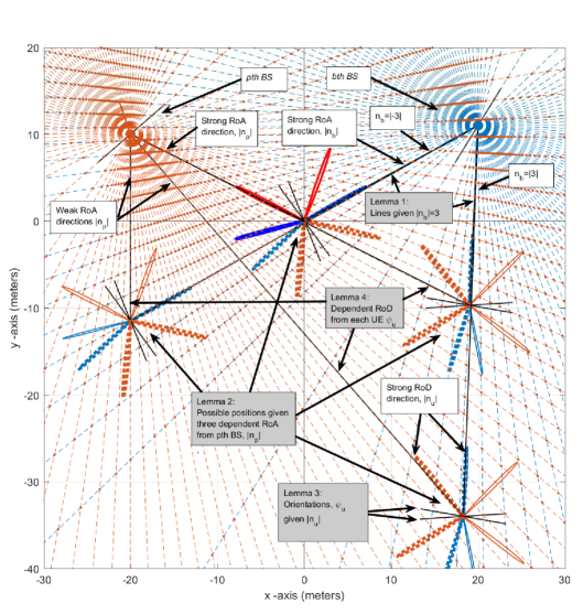
Figure 2: An example deployment model ($B=2$) showing the set of bipolar ray-based rays-of-arrival (RoAs)extending from each BS as dashed lines. In this example, the true user equipment (UE)position is shown at the origin, with bold-solid beam patterns depicting the ray-of-reparture (RoD)directions expected to have strong gains. The scenario illustrated here is conditional upon the true $n_{u}$ and $n_{b}$. As such, the other UE positions and pairs of orientations show the conditional rotation of the correct directions. It is evident that the origin UE position aligns both $n_{b}$ and the conditionally dependent $n_{p}$. Therefore, both $\bm{V}^{(b)}_{|n_{b}|,|n_{u}|}$ and $\bm{V}^{(p)}_{|n_{p}|,|n_{u}|}$ would be expected to be strong. In each other position, either one or all of the directions do not align, and thus they correspond to expected weak codependent pairs for each virtual channel. In particular, the geometry of the lower right-hand UE position does result in the correct alignment of each AoD and will therefore index the correct columns of both $\bm{V}^{(b)}$ and $\bm{V}^{(p)}$. However, as the RoA to the $p$th BS is misaligned, the resulting joint probability will be low. Furthermore, the expected channel gain for this distant position will be significantly lower than the one observed from the true UE position at the origin.

From (29), recall that, after the UE has finished transmitting its sequence of pilot symbols, each BS is able to make an independent estimate of the up-link channel. In this sub-section, we consider that the $b$th BS has its own estimate, denoted by $\hat{\bm{V}}^{(b)}$, and also has access to the estimated virtual channel from the $p$th BS, denoted as $\hat{\bm{V}}^{(p)}$. Leveraging the model developed in the previous sub-sections, we now aim to utilize the mutual dependency among virtual channel entries to find the joint probability of each direction. In doing so, we therefore collectively increase overall network performance.

We begin by considering a single entry of the $b$th BS’s virtual channel ${\bm{V}}^{(b)}_{n_{b},n_{u}}$, which here denotes the estimated path gain between the $n_{b}$th BS candidate beamforming vector $n_{u}$th and the UE candidate beamforming vector. From (12)-(13), we can therefore elaborate this particular entry as

$${\bm{V}}^{(b)}_{n_{b},n_{u}}=\frac{1}{\sqrt{N_{\!U\!E}N_{\!B\!S}}}(\bm{w}_{c}(n_{b}))^{H} {\bm{H}}^{(b)}\bm{f}_{c}(n_{u}).$$ (74)

By recalling (6), we can then consider the conditional probability density function (PDF) of the channel in (74), given the channels AoD and AoA that are perfectly aligned with the beamforming vectors $\bm{f}_{c}(n_{u})$ and $\bm{w}_{c}(n_{b})$ i.e., $\theta^{L}_{b}\in\{-\bar{\theta}_{n_{b}},\bar{\theta}_{n_{b}}\}$ and $\phi^{L}_{b}\in\{-\bar{\phi}_{n_{u}},\bar{\phi}_{n_{u}}\}$. From (6), we can substitute these angles into (74) to yield

$$f({\bm{V}}^{(b)}_{n_{b},n_{u}}|n_{b},n_{u}) =f(\alpha_{b}(\bm{w}_{c}(n_{b}))^{H}\bm{a}_{B\!S}\big{(}\pm\bar{\theta}_{n_{b}}\big{)}\big{(}\bm{a}_{U\!E}(\pm\bar{\phi}_{n_{u}}\big{)})^{H}\bm{f}_{c}(n_{u})|n_{b},n_{u})$$

$$=f(\alpha_{b}|n_{b},n_{u}).$$ (75)

By itself, this conditional destiny function is the same as that used in independent estimation, with the PDF of $\hat{\alpha}_{b}$ being limited to $f(\alpha_{b}|r_{b})\sim\mathcal{C}\mathcal{N}(0,r_{b}^{-\beta})$ for some unknown radial distance, $r_{b}$. However, by utilizing the models developed in the previous sub-sections, we are now able to consider (III-F) all available information and extend each conditional $n_{b}$ and $n_{u}$ into the global deployment, namely by considering the implication of each conditional for all other BS.

By recalling array orientations and the resulting relationship between the global and local angles as $\phi^{L}_{b}=\phi^{G}_{b}-\psi_{u},\forall\;b=1,\cdots,B$, and $\theta^{L}_{b}=\theta^{G}_{b}-\Theta_{b},\forall\;b=1,\cdots,B$, we can deduce the following conditionally related angle sets.

Theorem 1 ( RAPID Theorem of Mutually Dependent Beam Angles):

If the channel between the UE and the $b$th BS has a LOS propagation path such that $\theta^{L}_{b}\in\{-\bar{\theta}_{n_{b}}$ and $\bar{\theta}_{n_{b}}\}$ and $\phi^{L}_{b}\in\{-\bar{\phi}_{n_{u}},\bar{\phi}_{n_{u}}\}$ with a corresponding virtual channel density function, as described by (III-F), then for the $p$th BS to have jointly a LOS path to the same UE, it follows that the $p$th BS must also have

$$f\left(\frac{(\bm{w}_{c}(|\ddot{n}_{p}|))^{H}\hat{\bm{H}}^{(p)}\bm{a}_{U\!E}(\phi^{L}_{p}(\ddot{n}_{b},\ddot{n}_{p},n_{u})\big{)}}{\sqrt{N_{\!U\!E}N_{\!B\!S}}}\Bigg{|}n_{b},n_{u}\right)=f(\alpha_{p}|n_{b},n_{u}),$$

$$\qquad\qquad\forall\;\ddot{n}_{p}\in\mathcal{R}_{\ddot{n}_{b}}^{(p)}|\exists\;\mathcal{R}_{\ddot{n}_{b}}^{(p)}\;\forall\;\ddot{n}_{b}\in\{-n_{b},n_{b}\},\ddot{n}_{u}\in\{-n_{u},n_{u}\}$$ (76)

where the conditional AoD to the $p$th BS, $\phi^{L}_{p}(\ddot{n}_{b},\ddot{n}_{p},n_{u})$, satisfies the relationship

$$\phi^{L}_{p}(\ddot{n}_{b},\ddot{n}_{p},n_{u})=\text{atan2}(r_{b}(\ddot{n}_{b},\ddot{n}_{p})\;{R}_{y}(\ddot{n}_{b})-\delta_{y_{p,b}},$$

$$r_{b}(\ddot{n}_{b},\ddot{n}_{p})\;{R}_{x}(\ddot{n}_{b})-\delta_{x_{p,b}})+$$

$$\bar{\theta}_{\ddot{n}_{b}}+\bar{\phi}_{\ddot{n}_{u}}+\Theta_{b}.$$ (77)

•        Lemma 1.1 ( Conditional Line Dependency):

  In order for the $b$th BS to receive pilot signals with the $n_{b}$th candidate beam, the propagation source (i.e., the UE) must be positioned at some point along the RoA line, indexed by $n_{b}=|\ddot{n}_{b}|,\forall\;\ddot{n}_{b}\in\{-n_{b},n_{b}\}$.

         Lemma 1.2 ( Mutually Observable Positions):

  For the $p$th BS to have jointly received pilot signals from the same propagation source, from (72) it follows that there must exist some RoA index that satisfies $\ddot{n}_{p}\in\mathcal{R}_{\ddot{n}_{b}}^{(p)},\forall\;\ddot{n}_{b}\in\{-n_{b},n_{b}\}$. That is, there must be some RoA line extending from the $p$th BS that intercepts with the $b$th BS’s RoA, indexed by $\ddot{n}_{b}\in\{-n_{b},n_{b}\}$. Furthermore, this intercept has a relative displacement of $(\tilde{x}_{b},\tilde{y}_{b})\in\bm{\mathcal{P}}_{\ddot{n}_{b}}^{(p)}$ from the $b$th BS.

         Lemma 1.3 ( Mutual Orientation Dependency):

  In order for this common propagation source to qualify as being a line of sight path from the UE, the orientation of the UE must direct the conditionally considered $n_{u}$th candidate beam toward the $b$th BS. In other words, it must satisfy the relationship $\phi^{G}_{b}=\pi-\theta^{G}_{b}$, which leads to the condition that the UE orientation must be one of $\psi_{u}=\pi-\theta^{L}_{b}-\Theta_{b}-\phi^{L}_{b},\forall\;\theta^{L}_{b}\in\{-\bar{\theta}_{n_{b}},\bar{\theta}_{n_{b}}\},\;\phi^{L}_{b}\in\{-\bar{\phi}_{n_{u}},\bar{\phi}_{n_{u}}\}$.

         Lemma 1.4 ( Conditional RoD):

  For the UE to have jointly a LOS path to the $p$th BS (i.e., from $(\tilde{x}_{b},\tilde{y}_{b})$ to ($\delta_{x_{p,b}},\delta_{y_{p,b}}$), relative to the $b$th BS), it must have a global AoD that satisfies $\phi^{G}_{p}=\text{atan2}(\delta_{y_{p,b}}-\tilde{y}_{b},\delta_{x_{p,b}}-\tilde{x}_{b}),\forall\;(\tilde{x}_{b},\tilde{y}_{b})\in\bm{\mathcal{P}}_{\ddot{n}_{b}}^{(p)}$. With orientation $\psi_{u}$ from Lemma 1.3, the local AoD can then be expressed as $\phi^{L}_{p}(\ddot{n}_{b},\ddot{n}_{p},n_{u})=\phi^{G}_{p}-\psi_{u}$ and therefore as elaborated in (1).

         Lemma 1.5 ( Conditional Radial Displacement and Path PDF):

  If the $b$th BS and $p$th BS have jointly LOS paths to a UE positioned at the intercepting point between the RoA pair $\ddot{n}_{b}$ and $\ddot{n}_{p}$, then, from (70-71), the UE radial distance is given by $r_{b}(\ddot{n}_{b},\ddot{n}_{p})$ for the $b$th BS and $r_{p}(\ddot{n}_{b},\ddot{n}_{p})$ for the $p$th BS. Next, the conditional likelihood function for a $b$th BSs path coefficient can be expressed as

  $$f(\hat{\alpha}_{b}|r_{b}(\ddot{n}_{b},\ddot{n}_{p})) =\frac{\text{exp}\left(\frac{-|\hat{\alpha}_{b}|^{2}}{r_{b}(\ddot{n}_{b},\ddot{n}_{p})^{-\beta}+\text{Var}[\hat{\alpha}_{b}])}\right)}{\pi(\;r_{p}(\ddot{n}_{b},\ddot{n}_{p})^{-\beta}+\text{Var}[\hat{\alpha}_{b}]))}$$ (78)

  and the path coefficient of $b$th BS as

  $$f(\hat{\alpha}_{p}| r_{p}(\ddot{n}_{b},\ddot{n}_{p}))=\frac{\text{exp}\left(\frac{-|\hat{\alpha}_{p}|^{2}}{r_{p}(\ddot{n}_{b},\ddot{n}_{p})^{-\beta}+\text{Var}[\hat{\alpha}_{p}])}\right)}{\pi(\;r_{p}(\ddot{n}_{b},\ddot{n}_{p})^{-\beta}+\text{Var}[\hat{\alpha}_{p}])}.$$ (79)

       Corollary 1.1:

From 1, we can use Bayes’ rule to obtain the conditional probability of $r_{b}(\ddot{n}_{b},\ddot{n}_{p})$ as

$$Pr( r_{b}(\ddot{n}_{b},\ddot{n}_{p})|\hat{\alpha}_{b})=\frac{f(\hat{\alpha}_{b}|r_{b}(\ddot{n}_{b},\ddot{n}_{p}))}{f(\hat{\alpha}_{b}|r_{b}(\ddot{n}_{b},\ddot{n}_{p}))+f(\hat{\alpha}_{b}|\neg r_{b}(\ddot{n}_{b},\ddot{n}_{p}))}$$ (80)

$$=\frac{1}{1+\frac{f(\hat{\alpha}_{b}|\neg r_{b}(\ddot{n}_{b},\ddot{n}_{p}))}{f(\hat{\alpha}_{b}|r_{b}(\ddot{n}_{b},\ddot{n}_{p}))}}$$ (81)

$$=\frac{1}{1+\big{(}\frac{r_{b}(\ddot{n}_{b},\ddot{n}_{p})^{-\beta}}{\text{Var}[\hat{\alpha}_{b}]}+1\big{)}\text{exp}\left(\frac{-|\hat{\alpha}_{b}|^{2}/\text{Var}[\hat{\alpha}_{b}]}{(1+\text{Var}[\hat{\alpha}_{b}]/r_{b}(\ddot{n}_{b},\ddot{n}_{p})^{-\beta})}\right)}$$ (82)

and similarly for $Pr(r_{p}(\ddot{n}_{b},\ddot{n}_{p})|\hat{\alpha}_{p})$. By considering that the conditional occurrence of events $r_{b}(\ddot{n}_{b},\ddot{n}_{p})$ and $r_{b}(\ddot{n}_{b},\ddot{n}_{p})$ is, by definition, completely dependent, we can express the probability of their intersection as

$$Pr(\ddot{n}_{b},\ddot{n}_{p}|\hat{\alpha}_{b},\hat{\alpha}_{p}) =Pr(r_{b}(\ddot{n}_{b},\ddot{n}_{p})\cap r_{p}(\ddot{n}_{b},\ddot{n}_{p})|\hat{\alpha}_{b},\hat{\alpha}_{p})$$ (83)

$$=Pr(r_{b}(\ddot{n}_{b},\ddot{n}_{p})|\hat{\alpha}_{b})Pr(r_{p}(\ddot{n}_{b},\ddot{n}_{p})|\hat{\alpha}_{p})\underline{}$$ (84)

and the union among all mutually exclusive solutions $\ddot{n}_{p}\in\mathcal{R}_{\ddot{n}_{b}}^{(p)}$ that are jointly conditioned with $\ddot{n}_{b}$ as

$$Pr(\ddot{n}_{b}|\hat{\alpha}_{b},\hat{\alpha}_{p})=Pr\Big{(}\;\underset{\ddot{n}_{p}\in\mathcal{R}_{\ddot{n}_{b}}^{(p)}}{\bigcup}\ddot{n}_{b},\ddot{n}_{p}|\hat{\alpha}_{b},\hat{\alpha}_{p}\Big{)}\frac{1}{|\mathcal{R}_{\ddot{n}_{b}}^{(p)}|}\underset{\ddot{n}_{p}\in\mathcal{R}_{\ddot{n}_{b}}^{(p)}}{\sum}Pr(\ddot{n}_{b},\ddot{n}_{p}|\hat{\alpha}_{b},\hat{\alpha}_{p})$$ (85)

Finally, by substituting the conditional path estimates $\hat{\alpha}_{b}=\hat{\bm{V}}^{(b)}_{n_{b},n_{u}}$ and $\hat{\alpha}_{p}=(\bm{w}_{c}(|\ddot{n}_{p}|))^{H}\bm{W}_{c}\hat{\bm{V}}^{(p)}\bm{F}_{c}^{H}\bm{a}_{U\!E}(\phi^{L}_{p}(\ddot{n}_{b},\ddot{n}_{p},n_{u})\big{)}$, and by approximating the estimation variance as being dominated by the AWGN noise components, i.e., $\text{Var}[\hat{\alpha}_{p}]=\text{Var}[\hat{\alpha}_{b}]=N_{0}$, we can consider this probability across each of the equiprobable ranges $|{n}_{b}|=\ddot{n}_{b}\in\{-n_{b},n_{b}\},|{n}_{u}|=\ddot{n}_{u}\in\{-n_{u},n_{u}\}$ to obtain

$$Pr(n_{b},n_{u}|\hat{\bm{V}}^{(b)},\hat{\bm{V}}^{(p)}) =\frac{1}{4}\sum_{\begin{subarray}{c}\!\ddot{n}_{b}\in\{-n_{b},n_{b}\}\\ \ddot{n}_{u}\in\{-n_{u},n_{u}\!\}\end{subarray}}Pr(\ddot{n}_{b}|\hat{\alpha}_{b},\hat{\alpha}_{p})$$ (86)

$$=\sum_{\begin{subarray}{c}\!\ddot{n}_{b}\in\{-n_{b},n_{b}\}\\ \ddot{n}_{u}\in\{-n_{u},n_{u}\!\}\end{subarray}}\underset{\ddot{n}_{p}\in\mathcal{R}_{\ddot{n}_{b}}^{(p)}}{\sum}\frac{1}{4|\mathcal{R}_{\ddot{n}_{b}}^{(p)}|}Pr(r_{p}(\ddot{n}_{b},\ddot{n}_{p})\Big{|}{\hat{\bm{V}}}^{(b)}_{n_{b},n_{u}})\times$$

$$\qquad Pr\left(r_{p}(\ddot{n}_{b},\ddot{n}_{p})\big{|}(\bm{w}_{c}(|\ddot{n}_{p}|))^{H}\bm{W}_{c}\hat{\bm{V}}^{(p)}\bm{F}_{c}^{H}\bm{a}_{U\!E}(\phi^{L}_{p}(\ddot{n}_{b},\ddot{n}_{p},n_{u})\big{)}\right)$$ (87)

where $\phi^{L}_{p}(\ddot{n}_{b},\ddot{n}_{p},n_{u})$ can be found from (1).

       Example 1.1:

An example that illustrates conditional geometry is shown in Fig. 2. Specifically, we show four conditional UE positions and orientations, given the RoA $\ddot{n}_{b}=3$ and $\ddot{n}_{b}=-3$ from the right-hand BS. As is the case in our system model, the true UE position is shown in the center (i.e., $\ddot{n}_{b}=-3$ in the example), with the correct RoD directions shown as the beamforming directions with bold-solid lines (i.e., $\ddot{n}_{u}$). It follows that the correct directions will be expected to correspond to virtual channel entries that exhibit a strong path gain. The dashed and solid lines shown for the other conditional UE positions represent the two possible UE array orientations, each of which results in the considered correct beamforming vector (i.e., the expected strong estimate) directed back toward the right-hand BS at (20,10). Focusing on the UE in the center, it is notable that one of the two array orientations perfectly aligns the correct beamforming direction toward the left-hand BS (i.e., it corresponds to the expected strong measurement in both virtual channels). As such, the probability of the conditional virtual channel entry will be high.

In contrast to the correct estimate, we can consider the alternative conditional UE positions at coordinates (-20,-12.5) and (-18.5,12.5). At these positions, it is evident that neither of two conditional orientations direct the observed strong beamforming directions toward to the true BS positions. As such, these candidate positions will yield low probabilities, as the expected measurements will not agree with the observed measurements. Focusing on the bottom-right UE position, we see that one of the two orientations does result in the alignment of the strong UE beamforming directions. However, as the resulting RoA from the left-hand BS is now incorrect, it will still correspond to a virtual channel entry with a weak gain and therefore result in low conditionally probability.

       Note 1.1:

It is worth noting that the geometric reasoning in Theorem 1 intentionally considers the scenario that applies to a joint LOS—as asserted through Lemmas (1.2)-(1.4). This set of conditions collectively considers geometric properties that would be consistent with a common line of sight path among two BS. In order to extend this framework to one that jointly estimates NLOS paths, the developed model could also consider common scatterers alongside the already considered LOS components. More specifically, for NLOS, it may also be considered that, for the intercept of two RoA pairs as a common NLOS propagation source (i.e., a scatterer), the RoD from the UE must be the same, or very similar, for both BS estimates. We have left this extension as future work.

III-G RAPID Summary

Leveraging the expressions from the previous sub-sections, we now give a complete description our RAPID beam training algorithm. We propose that after each BS has collected UE pilot symbols for $T_{E}$ channel estimation time slots, they each carry out their own channel estimation, before exchanging their estimates with nearby BS. Initially, we assume that this information exchange is made possible by either a wired/wireless front-haul link between each BS. We then propose a bandwidth limited exchange later in this sub-section.

Following (86), after each BS has exchanged its initial set of virtual channel estimates, the $b$th BS can then compute its a priori virtual channel probabilities as

$$Pr(n_{b},n_{u})=\frac{1}{B-1}\sum\limits_{\begin{subarray}{c}\;p=1,\\ p\neq b\end{subarray}}^{B}Pr(n_{b},n_{u}|\hat{\bm{V}}^{(b)},\hat{\bm{V}}^{(p)}).$$ (88)

With this result, each BS can then select those UE/BS candidate beamforming pairs which have greatest probability of a path for data communication. The BS can then feed back the selected UE candidate beamforming indexes, requiring just $\text{log}_{2}(N)$ per index, for use in the following data communication.

The achievable link rate between the UE and each BS can then be expressed as [18]

$$R_{opt}^{(u)}=\text{log}_{2}|\bm{I}+\frac{P}{N_{0}}\bm{W}_{d}^{H}\hat{\bm{H}}^{(b)}\bm{F}_{d}\bm{F}_{d}^{H}\hat{\bm{H}}^{H}\bm{W}_{d}|.$$ (89)

where $\bm{W}_{d}^{H}$ and $\bm{F}_{d}$ are BS and UE beamforming matrices consisting of the candidate beamforming vectors selected for communication. The remainder of this section proposes bandwidth-constrained information sharing and the application of RAPID in downlink estimations.

a) Bandwidth Constrained Ray Passing

Due to the difficulties inherent in mmWave communication, and the cost of wired back-haul in dense networks, it is possible that any communication channels between BS links may be bandwidth-constrained. To reduce this overhead, we assume that each BS is only able to share a limited number of entries from a virtual channel estimate.

Fortunately, for any given BS pair, $\hat{\bm{V}}^{(b)}$ and $\hat{\bm{V}}^{(p)}$, the complete set of entries is not needed, as they do not all have statistical dependencies. More specifically, as the two BS exist in a 2D plane with RoA bounded by positive radial distances, only half of the total number of $|\ddot{\mathcal{N}}_{B}|=2N_{\!B\!S}$ RoA directions from one BS have any directional component in relation to another BS. As such, the largest number of ROAs that can have a mutual intercept between two BS is $(|\ddot{\mathcal{N}}_{B}|/2)^{2}=N_{\!B\!S}^{2}$. Mathematically, we can denote the entries of the $b$th BS’s virtual channel estimate that are passed to the $p$th BS as

$$\hat{\bm{V}}^{(b|p)}_{|\ddot{n}_{b}|,{n}_{u}}\Leftarrow\hat{\bm{V}}^{(b)}_{|\ddot{n}_{b}|,{n}_{u}},\forall\;\;n_{u},\ddot{n}_{b}|\exists\ddot{n}_{b}\in\mathcal{R}_{\ddot{n}_{p}}^{(p)},\forall\;\ddot{n}_{p}\in\ddot{\mathcal{N}}$$ (90)

Returning to bandwidth constrained sharing, in some BS deployments as little as half of these $N_{\!B\!S}^{2}$ RoA intercepts correspond to unique entries in the virtual channel matrix. For example, when $\Theta_{b}=\Theta_{p}=0$ and both BS are positioned on the x-axis, the ROAs that are able to have intercepts are half in the positive AoA range and half in the negative AoA. Recalling the ULA beam ambiguity problem (i.e., $\bm{a}_{B\!S}(\theta)=\bm{a}_{B\!S}(-\theta)$), the positive and negative angle ranges correspond to the same entries in the virtual channel matrix, due to the absolute index $|\ddot{\mathcal{N}}_{B}|$. In this case, only $N_{\!B\!S}N_{\!U\!E}/2$ entries need to be shared. Conversely, in other cases, such as when $\Theta_{b}=\Theta_{p}=0$ and both BS are positioned on the y-axis, the angular range with a radial component toward the other BS is either all positive or all negative, and thus all $N_{\!B\!S}N_{\!U\!E}$ entries are statistically relevant, to some extent.

For very large MIMO systems, this may still lead to an undesirable sharing overhead. Fortunately, owing to sparsity of the mmWave channel, many of the estimated virtual channel entries are approximately zero and therefore can be neglected with little loss of performance. As such, we propose that, from the already reduced sets of virtual channel entries in (90), only the $N_{d}$ most dominant entries are shared. As the geometric representation of the mmWave channel is inherently sparse, this has little effect on the performance of the system, provided $N_{d}$ is still greater than the number of paths. Furthermore, this also decreases computational complexity, as only RoA pairs of significance need to be considered.

1

2 $\mathbf{UE\;Input:}$ Each UE has a network-known candidate beamforming pilot sequence $\sqrt{P}N_{d}\bm{s}_{m}\bm{F}_{m},\forall\;m=1,\cdots,T_{E}$.

3

4$\mathbf{BS\;Input:}$ The orientation, $\Theta_{p}$, and relative position of nearby BS $\bm{\Delta}_{b,p},\forall\;p=1,\cdots,B$. Each BS has $N_{d}$, $N_{0}$, $\beta$, $A_{g}$ and knows $\bm{A}_{m}^{(b)}=(\bm{s}_{m}^{T}\bm{F}_{m}^{T}\bm{F}_{c}^{*})\otimes((\bm{W}_{m}^{(b)})^{H}\bm{W}_{c})\forall\;m=1,\cdots,T_{E}.$

5

6$\mathbf{Initialization:}$ Each BS pre-computes the RoA intercepts

7 $\;\mathcal{R}_{\ddot{n}_{b}}^{(p)}=\Big{\{}\ddot{n}_{p}\in\ddot{\mathcal{N}}_{B}\;\Big{|}r_{b}(\ddot{n}_{b},\ddot{n}_{p})>0\land r_{p}(\ddot{n}_{b},\ddot{n}_{p})>0\Big{\}},\forall p,\ddot{n}_{b}$

8

9 $\mathbf{Transmission\;and\;Independent\;Estimation:}$

10

11for $m=1,2,\cdots,T_{E}$ do

12       // UE Transmits beamformed pilots

13       $\bm{x}_{m}=\sqrt{\frac{P}{R_{\!U\!E}}}\bm{F}_{m}\bm{s}_{m}$

14      

15      for $b=1,2,\cdots,B$ do

16             // The $b$th BS receives with $\bm{W}_{m}$ to obtain

17             $\bm{y}^{(b)}_{m}=(\bm{W}_{m}^{(b)})^{H}(\bm{H}^{(b)}\bm{x}_{m}+\bm{q}_{m}^{(b)})$

18            

19       end for

20      

21 end for

22

23for $b=1,2,\cdots,B$ do

24       // The $b$th BS uses $\bm{y}^{(b)}=[\bm{y}^{(b)}_{1};\cdots;\bm{y}^{(b)}_{T_{E}}]$ and

25       $\bm{A}^{(b)}=[\bm{A}_{1}^{(b)};\cdots;\bm{A}_{T_{E}}^{(b)}]$ for independent sparse recovery:

26       $\;\;\;\;\hat{\bm{v}}^{(b)}=\underset{\bm{v}}{\operatorname{argmin}}\Big{[}||\bm{y}^{(b)}-A_{g}\bm{A}^{(b)}\bm{v}||_{2}^{2}+\gamma||\bm{v}||_{1}\Big{]}$

27      

28 end for

29 $\mathbf{Ray\;Passing\;and\;Indirect\;Estimation:}$

30 for $b=1,2,\cdots,B$ do

31       for $p=1,2,\cdots,B,|\;p\neq b$  do

32            

33            // The $b$th BS passes its $N_{d}$ strongest entries to the $p$th BS, which has a common RoA intercept as

34             $\hat{\bm{V}}^{(b|p)}_{|\ddot{n}_{b}|,{n}_{u}}\Leftarrow\hat{\bm{V}}^{(b)}_{|\ddot{n}_{b}|,{n}_{u}},\forall\;\;n_{u},\ddot{n}_{b}|\exists\ddot{n}_{b}\in\mathcal{R}_{\ddot{n}_{p}}^{(p)},\forall\;\ddot{n}_{p}\in\ddot{\mathcal{N}}$

35            

36            // The $b$th BS receives $N_{d}$ entries from the $p$th BS as

37            

38            $\tilde{\bm{V}}^{(p)}_{|\ddot{n}_{p}|,{n}_{u}}\Leftarrow\hat{\bm{V}}^{(p|b)}_{|\ddot{n}_{p}|,{n}_{u}},\forall\;n_{u},\ddot{n}_{p}|\exists\ddot{n}_{p}\in\mathcal{R}_{\ddot{n}_{b}}^{(b)},\forall\;\ddot{n}_{b}\in\ddot{\mathcal{N}}$

39            

40            // The $b$th BS computes its the conditional probability from (86)

41             $Pr(n_{b},n_{u}|\hat{\bm{V}}^{(b)},\tilde{\bm{V}}^{(p)})=\frac{1}{4}\sum_{\begin{subarray}{c}\!\ddot{n}_{b}\in\{-n_{b},n_{b}\}\\ \ddot{n}_{u}\in\{-n_{u},n_{u}\!\}\end{subarray}}Pr(\ddot{n}_{b}|\hat{\alpha}_{b},\hat{\alpha}_{p}),\forall n_{b},n_{u}$

42            

43       end for

44      // Compute conditional probability given all other BS.

45       $Pr(n_{b},n_{u})=\frac{1}{4}\sum_{\begin{subarray}{c}p=1\\ p\neq b\end{subarray}}^{B}Pr(n_{b},n_{u}|\hat{\bm{V}}^{(b)},\tilde{\bm{V}}^{(p)}),\forall n_{b},n_{u}$

46      

47 end for

$\mathbf{Output:}$ $Pr(n_{b},n_{u})\forall n_{b},n_{u}$ .

Algorithm 1 Ray-of-Arrival Passing for In-Direct (RAPID)Beam Training.

Using this approach, we denote the constrained matrix received by the $b$th BS from the $p$th BS as $\tilde{\bm{V}}^{(p)}$, such that $||\tilde{\bm{V}}^{(p)}||_{0}=N_{d}$ as

$$\tilde{\bm{V}}^{(p)}_{|\ddot{n}_{p}|,{n}_{u}}\Leftarrow\tilde{\bm{V}}^{(p|b)}_{|\ddot{n}_{p}|,{n}_{u}},\forall\;n_{u},\ddot{n}_{p}|\exists\ddot{n}_{p}\in\mathcal{R}_{\ddot{n}_{b}}^{(b)},\forall\;\ddot{n}_{b}\in\ddot{\mathcal{N}}$$ (91)

With this constrained information, we can rewrite (88) as

$$Pr(n_{b},n_{u})=\frac{1}{B-1}\sum\limits_{\begin{subarray}{c}\;p=1,\\ p\neq b\end{subarray}}^{B}Pr(n_{b},n_{u}|\hat{\bm{V}}^{(b)},\tilde{\bm{V}}^{(p)}).$$ (92)

We show the complete RAPID beam training approach in Algorithm 1.

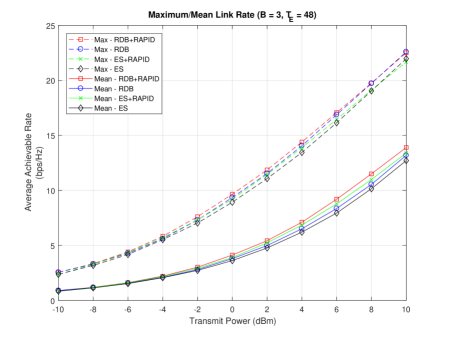
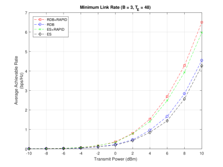
Figure 3: results where the network consists of $B=3$ base station (BS), each equipped with $N_{\!B\!S}=32$ antennas and $R_{\!B\!S}=8$ radio frequency (RF)chains and the user is equipped with $N_{\!U\!E}=16$ antennas and $R_{\!U\!E}=4$ RF chains. We assume the expected number of paths is $E[L]=3$. (a) Shows the average maximum and mean achievable link rates after estimation, while (b) shows the minimum achievable link rate.

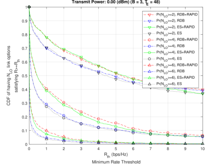
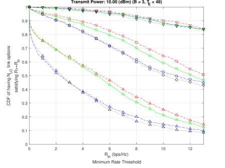
Figure 4: Numerical results where the network consists of $B=3$ base station (BS), each equipped with $N_{\!B\!S}=32$ antennas and $R_{\!B\!S}=8$ radio frequency (RF)chains and the user is equipped with $N_{\!U\!E}=16$ antennas and $R_{\!U\!E}=4$ RF chains. We assume the expected number of paths is $E[L]=3$. (c) shows the cumulative density function (CDF)of network coverage for $P=0$ dBm and (d) $P=10$ dBm.

b) RAPID Downlink Beam Training

Up to this point, we have introduced RAPID as a cooperative uplink channel estimation strategy; however, by considering that the only prior knowledge required to compute (88) is the relative positions of each network BS and their orientations, RAPID can also be implemented in downlink at the UE. To this end, the UE would only require this static network deployment information, along with a coarse estimate its network position, in order to reduce the number of considered BS. Then, similarly to the uplink description, each BS can broadcast beamformed pilot signals with orthogonal spreading codes while each UE collects the signals with a sequence of beamforming directions. After the $T_{E}$ estimation time slots, each UE can make a direct estimate of the downlink channel and implement RAPID with no communication overhead for the network.

In this scenario, although there is no sharing overhead, the computational burden that was originally in the up-link and distributed among several BS would now need to be carried out by a single UE. As the UE is expected to have less computational power and more stringent energy requirements, it may still be beneficial for the UE to only consider the $N_{d}$ most dominant and dependent entries from each estimate. This downlink estimation strategy would also still permit the UE to adapt its beamforming directions during the estimation process, as proposed in [24].

IV Numerical Results

We now provide some numerical results to evaluate the performance of our proposed scheme. We consider an mmWave system where a UE is equipped with $N_{\!U\!E}=16$ antennas and $R_{\!U\!E}=4$ RF chains. We assume this UE to be within the range of a network of $B$ BS, each equipped with $N_{\!B\!S}=32$ antennas and $R_{\!B\!S}=8$ RF chains. We adopt a user-centric deployment network model in which each BS is positioned within a $100$m x $100$m grid, with the UE at its center (i.e., a maximum of $50$m away from the UE along the x- or y-axis). We consider each BS to follow a uniform random distribution within this space, while the orientation of each BS also follows a uniformly random distribution in the continuous range $[0,2\pi]$. Similarly, we consider UE orientation to also follow a uniform random distribution in the range $[0,2\pi]$. The resulting deployment dependent channels can therefore be found from (10), in which the path loss exponent is considered as $\beta=4$ to represent severe mmWave propagation losses. We consider each receiver’s noise power to be $N_{0}=10^{-5}$, such that the propagation path signal-to-noise ratio (SNR) can be expressed as $\sigma_{R}^{2}/N_{0}$, which leads to a minimum link SNR of $r_{b}^{-\beta}/N_{0}=-24$ dB at $\text{max}[r_{b}]=\sqrt{2}\times 50m$.

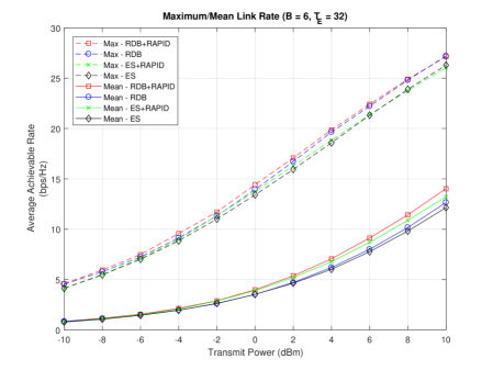
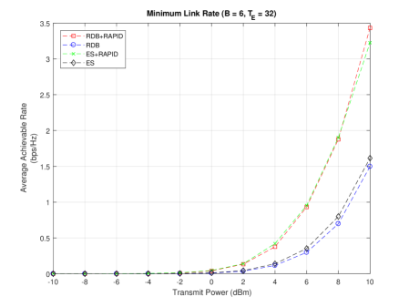
Figure 5: Numerical results where the network consists of $B=6$ base station (BS), each equipped with $N_{\!B\!S}=32$ antennas and $R_{\!B\!S}=8$ radio frequency (RF)chains and the user is equipped with $N_{\!U\!E}=16$ antennas and $R_{\!U\!E}=4$ RF chains. (a) Shows the average maximum and mean achievable link rates after estimation, while (b) shows the minimum achievable link rate.

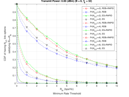
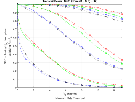
Figure 6: Numerical results where the network consists of $B=6$ base station (BS), each equipped with $N_{\!B\!S}=32$ antennas and $R_{\!B\!S}=8$ radio frequency (RF)chains and the user is equipped with $N_{\!U\!E}=16$ antennas and $R_{\!U\!E}=4$ RF chains. (c) shows the cumulative density function (CDF)of network coverage for $P=0$ dBm and (d) $P=10$ dBm.

We apply RAPID to RDB with $T_{E}$ channel estimation time slots and an ES-based channel estimation with $T_{ES}=N_{\!U\!E}N_{\!B\!S}/R_{\!B\!S}=64$ estimation time slots. To compare the performance of each scheme as a result of estimation, we show the average best-available link rate (i.e., the maximum achievable rate given all estimated channels) along with the average of the worst available link rate (i.e., the minimum achievable link rate given all estimated channels). For completeness, we also include the average of all available links. To demonstrate coverage probability and link redundancy, we also show the cumulative density function (CDF) of the UE with $N_{LO}$ link options, whereby we impose the requirement that a link must satisfy $R>R_{th}$ along with a coverage rate threshold $R_{th}$.

In Fig. 3 (a), we show both the maximum achievable link rate and the average achievable link rate for a network of $B=3$ BS, with RDB using $T_{E}=48$. In most cases, it is evident that RDB tends to outperform ES despite using fewer measurement timeslots, particularly at a high SNR, because RDB has greater measurement diversity due to pilots being transmitted with multiple beamforming directions in each time slot. This effectively allows the receiver to sample several entries of the virtual channel at once. Conversely, ES sequentially transmits a pilot with only one beamforming direction at a time and is included as a benchmark approach. By comparing the average link rate of the schemes in Fig. 3 (a), it is notable that those using RAPID show little advantage at a low SNR; however, as transmit power increases, both ES and RDB are able to achieve an average link rate increase of around 1 bit/s/Hz. Interestingly, comparing this to maximum link rate performance, we find that the there is very little increase as SNR increases, because—in most cases—the BS that has the best channel in relation to the UE is the one that stands to gain the least from sharing its information with the other BS. Conversely, in Fig. 3 (b), we show the average of the minimum achievable link rate, which effectively represents the BS that has the worst channel in relation to the UE, which is therefore the BS that stands to gain the most from exchanging information. As the UE transmit power increases, we can see that the minimum link rate of the systems using RAPID increase significantly by up to around 2bps/Hz at a transmit power of 10 dBm.

Turning our attention to Figs. 4 (a) and (b), we show the CDFs for a number of achievable link options, for $P=0$ dBm and $P=10$ dBm, respectively. In both cases, we can see that RAPID is able to increase significantly the probability of having a larger number of available link options, particularly for lower-rate requirement thresholds. This is an inherent property of RAPID’s ability to improve significantly the weaker network links. This low rate threshold region also fits for mmWave systems, as throughput gains are expected to come from large bandwidths as opposed to complex modulation schemes. For much greater rate thresholds we see that the available link probabilities of all systems tend to converge.

In Fig. 5 and Fig. 6, we increase BS density to $B=6$ for the same deployment area. We also reduce the number of RDB time slots to $T_{E}=32$. In (a) and (b), we again show the minimum, mean, and maximum link rates. Again, we can see from (b) that the minimum link rate is able to increase by around 2 bits/s/Hz by applying RAPID despite the worst of the $B=6$ channels being much worse than $B=3$, as in Fig. 3. Looking at the average link rate in Fig. 5 (b), we can see a more noticeable increase with $B=6$ for the same reason, as now there are many more BS to benefit from the the better channels that are shared. Turning to the CDFs in 6 (a) and (b), we find that the probability of having more available links is still much greater with RAPID, in particular at a high SNR.

V Conclusion

In this paper we proposed have a cooperative mmWave beam training scheme in which multiple network BS share information to enhance the channel estimation accuracy of one another—and therefore the network performance as whole. In order to combine shared information, we proposed a Ray-of-Arrival Passing for In-Direct (RAPID)algorithm in which the probability of each directional path can be conditionally considered by multiple BS. By leveraging the derived statistical relations, it was proposed that each BS need only share information with other BS that are able to utilize it, thus reducing the communication overhead involved in this information sharing. The presented results established that the BS link which has the worst quality benefits the most from the scheme. Furthermore, by considering a minimum rate threshold for communication, we demonstrated that RAPID is able to increase significantly the probability that one or more links are available to a user at any given time.

References

- [1] X. Ge, S. Tu, G. Mao, C.-X. Wang, and T. Han, “5G ultra-dense cellular networks,” IEEE Trans. Wireless Commun., vol. 23, no. 1, pp. 72–79, 2016.
- [2] R. Baldemair, T. Irnich, K. Balachandran, E. Dahlman, G. Mildh, Y. Selén, S. Parkvall, M. Meyer, and A. Osseiran, “Ultra-dense networks in millimeter-wave frequencies,” IEEE Commun. Mag., vol. 53, no. 1, pp. 202–208, 01 2015.
- [3] S. Chen, F. Qin, B. Hu, X. Li, and Z. Chen, “User-centric ultra-dense networks for 5G: challenges, methodologies, and directions,” IEEE Trans. on Wireless Commun., vol. 23, no. 2, pp. 78–85, April 2016.
- [4] C. Yang, J. Li, and M. Guizani, “Cooperation for spectral and energy efficiency in ultra-dense small cell networks,” IEEE Trans. on Wireless Commun., vol. 23, no. 1, pp. 64–71, February 2016.
- [5] T. Bai, A. Alkhateeb, and R. Heath, “Coverage and capacity of millimeter-wave cellular networks,” IEEE Commun. Mag., vol. 52, no. 9, pp. 70–77, 2014.
- [6] M. N. Kulkarni, S. Singh, and J. G. Andrews, “Coverage and rate trends in dense urban mmwave cellular networks,” IEEE GLOBECOM, pp. 3809–3814, 2014.
- [7] T. Bai and R. W. Heath., “Coverage and rate analysis for millimeter-wave cellular networks,” IEEE Trans. on Wireless Commun., pp. 1100–1114, 2015.
- [8] T. S. Rappaport, S. Sun, R. Mayzus, H. Zhao, Y. Azar, K. Wang, G. N. Wong, J. K. Schulz, M. Samimi, and F. Gutierrez, “Millimeter wave mobile communications for 5G cellular: It will work!” IEEE Access, vol. 1, pp. 335–349, 2013.
- [9] C. Dehos, J. L. González, A. De Domenico, D. Kténas, and L. Dussopt, “Millimeter-wave access and backhauling: the solution to the exponential data traffic increase in 5G mobile communications systems?” IEEE Commun. Mag., vol. 52, no. 9, pp. 88–95, 2014.
- [10] G. MacCartney and T. Rappaport, “73 GHz millimeter wave propagation measurements for outdoor urban mobile and backhaul communications in New York City,” in IEEE Int. Conf. on Commun. (ICC), June 2014, pp. 4862–4867.
- [11] P. Popovski, “Ultra-reliable communication in 5G wireless systems,” in Int. Conf. on 5G for Ubiquitous Connectivity, Nov 2014, pp. 146–151.
- [12] T. Levanen, J. Pirskanen, and M. Valkama, “Radio interface design for ultra-low latency millimeter-wave communications in 5G era,” in IEEE GLOBECOM, Dec 2014, pp. 1420–1426.
- [13] W. Roh, J.-Y. Seol, J. Park, B. Lee, J. Lee, Y. Kim, J. Cho, K. Cheun, and F. Aryanfar, “Millimeter-wave beamforming as an enabling technology for 5G cellular communications: theoretical feasibility and prototype results,” IEEE Commun. Mag., vol. 52, no. 2, pp. 106–113, 2014.
- [14] F. Khan, Z. Pi, and S. Rajagopal, “Millimeter-wave mobile broadband with large scale spatial processing for 5G mobile communication,” in 2012 50th Annual Allerton Conference on Communication, Control, and Computing (Allerton), Oct 2012, pp. 1517–1523.
- [15] H. Shokri-Ghadikolaei, F. Boccardi, E. Erkip, C. Fischione, G. Fodor, M. Kountouris, P. Popovski, and M. Zorzi, “The impact of beamforming and coordination on spectrum pooling in mmwave cellular networks,” in 2016 50th Asilomar Conference on Signals, Systems and Computers, Nov 2016, pp. 21–26.
- [16] A. Sayeed, “Deconstructing multiantenna fading channels,” IEEE Trans. Sig. Process., vol. 50, no. 10, pp. 2563–2579, Oct. 2002.
- [17] J. Brady, N. Behdad, and A. Sayeed, “Beamspace MIMO for millimeter-wave communications: System architecture, modeling, analysis, and measurements,” IEEE Trans. Antennas Propag., vol. 61, no. 7, pp. 3814–3827, July 2013.
- [18] A. Alkhateeb, O. El Ayach, G. Leus, and R. Heath, “Channel estimation and hybrid precoding for millimeter wave cellular systems,” IEEE J. Sel. Topics Signal Process., vol. 8, no. 5, pp. 831–846, Oct. 2014.
- [19] J. Wang, Z. Lan, C.-W. Pyo, T. Baykas, C.-S. Sum, M. Azizur Rahman, R. Funada, F. Kojima, I. Lakkis, H. Harada, and S. Kato, “Beam codebook based beamforming protocol for multi-gbps millimeter-wave WPAN systems,” in IEEE J. Select. Areas Commun., 2009, pp. 1390–1399.
- [20] Z. Xiao, T. He, P. Xia, and X.-G. Xia, “Hierarchical codebook design for beamforming training in millimeter-wave communication,” IEEE Trans. Commun., vol. 15, no. 5, pp. 3380–3392, 2016.
- [21] M. Kokshoorn, P. Wang, Y. Li, and B. Vucetic, “Fast channel estimation for millimetre wave wireless systems using overlapped beam patterns,” in IEEE Int. Conf. on Commun. (ICC), June 2015, pp. 1304–1309.
- [22] M. Kokshoorn, H. Chen, P. Wang, Y. Li, and B. Vucetic, “Millimeter wave MIMO channel estimation using overlapped beam patterns and rate adaptation,” IEEE Trans. Signal Process., vol. PP, no. 99, pp. 1–1, 2016.
- [23] M. Kokshoorn, H. Chen, Y. Li, and B. Vucetic, “RACE: A rate adaptive channel estimation approach for millimeter wave MIMO systems,” IEEE GLOBECOM, pp. 1–6, Dec 2016.
- [24] ——, “Beam-on-graph: Simultaneous channel estimation for mmwave MIMO systems with multiple users,” IEEE Trans. Commun., 2018.
- [25] ——, “Fountain code-inspired channel estimation for multi-user millimeter wave MIMO systems,” in IEEE Int. Conf. on Commun. (ICC), May 2017, to appear.
- [26] A. Alkhateeby, G. Leusz, and R. W. Heath, “Compressed sensing based multi-user millimeter wave systems: How many measurements are needed?” in 2015 IEEE ICASSP, 2015, pp. 2909–2913.
- [27] M. Giordani, M. Mezzavilla, S. Rangan, and M. Zorzi, “Multi-connectivity in 5G mmwave cellular networks,” in Mediterranean Ad Hoc Networking Workshop (Med-Hoc-Net), June 2016, pp. 1–7.
- [28] M. Giordani, M. Mezzavilla, and M. Zorzi, “Initial access in 5G mmwave cellular networks,” IEEE Commun. Mag., vol. 54, no. 11, pp. 40–47, November 2016.
- [29] M. Polese, M. Giordani, M. Mezzavilla, S. Rangan, and M. Zorzi, “Improved handover through dual connectivity in 5G mmwave mobile networks,” IEEE J. Sel. Areas in Commun., vol. 35, no. 9, pp. 2069–2084, Sept 2017.
- [30] H. Miao, K. Yu, and M. J. Juntti, “Positioning for nlos propagation: Algorithm derivations and cramer-rao bounds,” IEEE Trans. on Vehicular Tech., vol. 56, no. 5, pp. 2568–2580, Sept 2007.
- [31] T. S. Rappaport, J. H. Reed, and B. D. Woerner, “Position location using wireless communications on highways of the future,” IEEE Commun. Mag., vol. 34, no. 10, pp. 33–41, Oct 1996.
- [32] C. K. Seow and S. Y. Tan, “Non-line-of-sight localization in multipath environments,” IEEE Trans. on Mobile Comp., vol. 7, no. 5, pp. 647–660, May 2008.
- [33] H. Deng and A. Sayeed, “Mm-wave MIMO channel modeling and user localization using sparse beamspace signatures,” in IEEE SPAWC, June 2014, pp. 130–134.
- [34] A. Sayeed and V. Raghavan, “The ideal MIMO channel: Maximizing capacity in sparse multipath with reconfigurable arrays,” in IEEE Proc. ISIT, July 2006, pp. 1036–1040.
- [35] S. Rangan, “Generalized approximate message passing for estimation with random linear mixing,” in IEEE ISIT, 2011, pp. 2168–2172.
- [36] J. Vila and P. Schniter, “Expectation-maximization bernoulli-gaussian approximate message passing,” in IEEE Conf. on Signals, Systems and Computers, 2011, pp. 799–803.
- [37] J. Mo, P. Schniter, N. Gonzalez Prelcic, and R. Heath, “Channel estimation in millimeter wave MIMO systems with one-bit quantization,” in Proc. Conf. Signals, Syst. Comput., Nov 2014, pp. 957–961.