User-Sensitive Recommendation Ensemble with Clustered Multi-Task Learning

Abstract

This paper considers recommendation algorithm ensembles in a user-sensitive manner. Recently researchers have proposed various effective recommendation algorithms, which utilized different aspects of the data and different techniques. However, the “user skewed prediction” problem may exist for almost all recommendation algorithms – algorithms with best average predictive accuracy may cover up that the algorithms may perform poorly for some part of users, which will lead to biased services in real scenarios. In this paper, we propose a user-sensitive ensemble method named “UREC” to address this issue. We first cluster users based on the recommendation predictions, then we use multi-task learning to learn the user-sensitive ensemble function for the users. In addition, to alleviate the negative effects of new user problem to clustering users, we propose an approximate approach based on a spectral relaxation. Experiments on real-world datasets demonstrate the superiority of our methods.

1 Introduction

In recent years recommender systems have become increasingly popular, and various effective recommendation algorithms have been proposed. Currently one trend of recommendation research is to incorporate collaborative filtering with side information (e.g, social information Wang et al. (2017) and item reviews McAuley and Leskovec (2013)) and other promising techniques (e.g., deep learning Karatzoglou and Hidasi (2017) and transfer learning Weiss et al. (2016)).

However, few studies have focused on the “skewed prediction” problem, where the model with the best average predictive accuracy will leave meaningful subsets of users/items modeled significantly worse than other subsets Beutel et al. (2017). The “skewed prediction” problem may become a common drawback of the existing recommendation algorithms as they use average based metrics for evaluation. The globally optimal model is typically not the best model for all the users. We focus on the user skewness and show an illustrative experimental result on the public dataset MovieLens-100K in Figure 1. Traditionally we compare the average MSE of two algorithms, and from the left table we can easily tell the MF model is better. But if we analyze the MSE on user level, we can see that only 53.2% of users suit MF more than KNN. Directly deploying MF for real use will provide biased services to users. Besides the performance measurement, one important reason is user heterogeneity. Specifically, there are many types of users and an algorithm with predefined structure and techniques probably can not capture the preference of all types of users well, which accounts for the user skewed predictions. This problem may also exist among recent advanced recommendation algorithms. For example, social recommendation utilizes user’s social information to capture user preference, and it will underperform for the users who have few social friends. Tag-based recommendation also has similar problems as not all the users like to annotate tags.

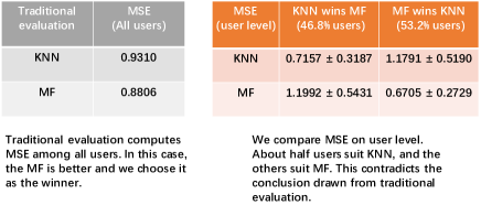
Figure 1: A comparison of mean square error (MSE) on two classical recommendation algorithms K-nearest neighbors (KNN) and Matrix Factorization (MF) on the MovieLens-100K dataset.

This paper considers recommendation ensembles to address this problem. Different algorithms may suit different types of users and a natural way to improve the recommendation performance is to combine them properly. Traditional ensemble methods (e.g., bagging, boosting, and stacking) often learn a weight for each base algorithm and apply it to all users, which, however, do not consider the user heterogeneity phenomenon and thus are not the optimal choice in the recommendation field. We assume that homogeneous users should share similar ensemble strategies as algorithms are expected to perform stably on homogeneous users. Then a natural idea is to divide users into several homogeneous groups by analyzing base algorithms and learn ensemble weights within each group. The intuition is clear and sensible: if recommendation algorithms have similar performances on some users, these users are more likely to be homogeneous and they should share similar weights during ensemble. This idea is very close to clustered multi-task learning Zhou et al. (2011) if we treat ensemble for each user as a single task. Users follow a clustered structure and users in the same group share parameters during task learning. Compared to a more personalized approach that learns ensemble for users individually, our method tends to be more reliable and can alleviate the data sparsity problem. We call this ensemble strategy is user-sensitive.

In this paper we propose a user-sensitive recommendation ensemble approach, named “UREC”, to address the “user skewed prediction” problem. The main contributions of our work are listed as follows: (1) We first cluster users into homogeneous groups, and then use multi-task learning to learn ensemble function strategies for the users. To our best knowledge, it is the first work to consider user heterogeneity in recommendation ensemble. (2) To alleviate the new user problem that will interfere with the user clustering, we propose an approximate approach based on a spectral relaxation of regularization. (3) We conduct extensive experiments on real-world datasets to verify the efficacy of our method. The experimental results demonstrate that UREC outperforms other baseline models.

2 Related Work

2.1 Multi-task Learning

Multi-task learning (MTL) Ando and Zhang (2005) is a machine learning method where multiple tasks are jointly learnt such that each of them benefits from each other. Several researchers have applied MTL to recommendation with different assumption on how to define a task and what to share among tasks. Ning and Karypis (2010) proposed a multi-task model for recommendation with Support Vector Regression. But they focused on the task on the individual level and only used rating information. Wang et al. (2013) utilized MTL to online collaborative filtering where the weight vectors of multiple tasks are updated in an online manner. These works assumed that all the tasks are related. However, we assume a more sophisticated group structure among users where users only share relatedness within the same group.

2.2 Recommendation Ensemble

Ensemble-based algorithms have been well studied to improve the prediction performance Polikar (2006), and are widely adopted in recommendation competitions, such as the Netflix Prize contest Sill et al. (2009); Koren (2009) and KDD Cups McKenzie et al. (2012). Typically, an ensemble method combines the results of different algorithms to obtain a final prediction. The most basic strategy is to acquire the final prediction based on the mean over all the prediction results or the majority votes. Some popular ensemble methods are linear regression, restricted boltzmann machines (RBM), and gradient boosted decision trees (GBDT) Polikar (2006). However, they assume users are homogeneous and use the same ensemble strategy to all the users. It is then desirable to develop a user-sensitive ensemble method to capture and make use of user heterogeneity, as we shall do next.

2.3 Hybrid Recommendation Algorithms

Another related field is hybrid recommendation. Different from recommendation ensembles that combines the results of different algorithms, hybrid recommendation aims to build a model with multiple recommendation techniques to achieve a higher performance. Hybrid recommendation models have shown competitive results. The most common hybrid recommendation is to combine collaborative filtering with other techniques like content based model Basilico and Hofmann (2004), clustering Hu et al. (2014), and Bayesian model Beutel et al. (2014). One potential drawback of hybrid recommendation is the model structure and inference rules will become sophisticated when more techniques come into consideration. However, our method combines multiple techniques in an ensemble approach that can avoid this problem.

3 User Sensitive Recommendation Ensemble

Symbol	Description
$Y_{ij}$	the rating user $i$ gives to item $j$
$X^{k}$	the full predicted matrix by algorithm $k$
$W$	the ensemble weight matrix that is $[w_{1},...,w_{N}]$
$A^{k}$	the $k$th base algorithm, $k\in[1,2,...,K]$
$Z$	user type (homogeneous group)
$\bar{w}_{z}$	the average ensemble weights of group $z$
$m^{k}_{i}$	metric performance of algorithm $k$ on user $i$
$d^{k}_{iq}$	distance between users $i$ and $q$ based on algorithm $k$
$\alpha,\beta$	the regularization parameters

Table 1: Notation

3.1 Problem Description

Suppose there are $N$ users and $M$ items, and $K$ recommendation algorithms. Let $Y\in\mathbb{R}^{N\times M}$ be the user-item rating matrix where $Y_{ij}$ represents the preference user $i$ towards item $j$. Note that in most cases the $Y$ is very sparse – most values in $Y$ are missing. For every recommendation algorithm $k$, there is a prediction matrix $X^{k}\in\mathbb{R}^{N\times M}$ that stores all the predicted preferences of $N$ users towards $M$ items. Ensemble learning is to find a model that can better predict $Y$ based on $\{X^{k}\}$ without revising the inner design of the $K$ recommendation algorithms. Existing studies ignored the difference between users and treated them with same weights. In this paper, we use an adaptive ensemble model for all users, and our goal is to improve the overall prediction accuracy of the ensemble model by developing user-sensitive model parameters for users. We give the notation in Table 1.

3.2 Proposed Model

We introduce the formalization of UREC and discuss intuitions in detail with probabilistic graphical models in Figure 2. Figure 2(a) shows relationships among user hidden types $Z$, user features $F$, recommendation algorithms $A$, and user-item rating matrix $Y$. User features $F$ are determined by the hidden user type Z, and predictions $X^{k}$ are generated by algorithms $A^{k}$ and user features $F^{k}$. Note that in reality $F^{k}$ is often a very small subset of $F$. Most current algorithms only use users’ historical ratings as input. When (some or all of) the features are not observable, they are integrated out in the graphical representation given in (a); as a consequence, $X^{k}$ and $Y$ will be conditionally dependent (even given $Z$), as shown by the dashed line in Figure 2(b). Our purpose is to leverage all $X^{k}$’s for a better prediction of $Y$, as supported by the dependence between al $X^{k}$’s and $Y$. This simplified graphical representation indicates that $P(Y|X^{K})=\sum_{z=1}^{Z}P(Y|X^{K},z)P(z)$, where $X^{K}=\{X^{k}\}$. Traditional ensemble methods assume users are homogeneous, that is $P(Y|X^{K})=P(Y|X^{K},Z)$, and use $P(Y|X^{K})$ for all users. In the case of heterogeneous users, $P(Y|X^{K},z)$ may be different for different $z$. So our UREC involves two steps: the first step is to divide users into $Z$ homogeneous groups and the second step is to learn automated ensemble strategies within each group. Alternatively we can use soft clustering like Gaussian mixture models so that we can model user homogeneity more continuously. However, the high dimensions of $X^{K}$ and $Y$ will make the probabilistic clustering hard to deal with. So here we apply a k-medoids method based on the performance of base algorithms, which is hard clustering and detailed in the next subsection. In the second step we choose linear mixtures with automated determined coefficients as the ensemble model, which can be further extended to other models like trees and neural networks.

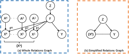
Figure 2: Relations graphs of recommendation.

3.3 Weighted User Grouping

In this section we introduce the weighted user grouping method, where the key is to define the user similarity. A common way is to calculate the distance (e.g., Euclidean, Pearson correlation) between user feature vectors to measure the similarity. We utilize both the algorithm predictions and user evaluations to define a proper user similarity measure. For each user pair $(i,q)$, we can get $K$ different distances based on predictions of $K$ algorithms, denoted by $\{d^{k}_{iq}\}$. To combine these distances together, we give each distance a confidence derived from the user performance of the base recommendation algorithms. Let $m^{k}_{i}$ be the performance indicator of $k$-th algorithm on user $i$: the smaller difference between $X^{k}_{i}$ and $Y_{i}$, the larger $m^{k}_{i}$. Then the final distance between user $i$ and $q$ is defined as:

$$d_{Final}(i,q)=\frac{\sum_{k=1}^{K}\frac{m^{k}_{i}+m^{k}_{q}}{2}d^{k}_{iq}}{\sum_{k=1}^{K}\frac{m^{k}_{i}+m^{k}_{q}}{2}}.$$ (1)

The algorithms that achieve higher performances on the two users will contribute more to the final distance. Besides, the choice of performance measure $m^{k}_{i}$ is flexible: We could select NDCG or Recall for top-N recommendation, or select MAE or RMSE for rating prediction. Note that in some metrics like MAE small values indicate high performances, we use the inverse of these metrics for $m^{k}_{i}$. With distance function defined, we use k-medoids method to group users.

3.4 Ensemble Learning with Grouped Users

For each user we learn a linear function $f_{i}(X^{K}_{i})=w^{T}_{i}X^{K}_{i}$ to combine the results. By now we have divided users into $Z$ groups; users within each group share similar parameters. Then the global empirical risk function we want to minimize becomes:

$$\begin{split}&\ L(W)=\sum\limits_{i=1}^{N}l(w^{T}_{i}X^{K}_{i*},Y_{i*})+\Omega(W),\\ &\ \Omega(W)=\alpha\sum\limits_{z=1}^{Z}\sum\limits_{v\in\mathbb{I}_{z}}\|w_{v}-\bar{w}_{z}\|^{2}+\beta\sum\limits_{z=1}^{Z}\|\bar{w}_{z}\|^{2},\\ \end{split}$$ (2)

where $l(\cdot,\cdot)$ is the loss function, $Y_{i*}$ indicates the ratings of user $i$ in the training data, $\Omega(W)$ is the regularization form and $W=[w_{1},...,w_{N}]$ is the weight matrix to be estimated, $\alpha$ and $\beta$ are the regularization parameters, $v\in\mathbb{I}_{z}$ means user $v$ is in the group $z$, and $\bar{w}_{z}$ is the average weights of group $z$. The first term in $\Omega(W)$ tries to enforce the grouping property of $w_{v}$. And the second term tries to avoid big values. Note that for flexibility we do not force all the users in the same group to have the same weight. However, the grouping information provides hints as to the similarities between the weights, this is clearly different from classical mixture of linear models Chaganty and Liang (2013), in which same groups use the same weights.

Although eq (2) is not convex, the minimization of each group is a convex problem. We can learn the ensemble weights separately when users are already grouped.

3.5 Incorporating New Users

In the weighted user grouping, we use prediction metrics for each user to derive $m^{k}_{i}$. However, new users who have few recorded ratings in $Y$ will interfere with the grouping phase as we can not accurately measure $m^{k}_{i}$. As a kind of cold start problem, the new user problem is a common challenge in recommendation area. To tackle this problem, we use an approximate approach based on a spectral relaxation form of eq (2). Specifically, the relaxation is based on regularization with spectral functions of matrices and transforms eq (2) to a convex problem. Instead of clustering users explicitly, this method implicitly clusters users by the constraints of the convex problem during learning the ensemble weights $W$. Thus it does not need $m^{k}_{i}$ for each user and can address the new user problem. Following the work of Ding and He (2004), we first reformulate the regularization $\Omega(W)$ to:

$$\Omega(W,F)=\alpha(\operatorname{Tr}(W^{T}W)-\operatorname{Tr}(F^{T}W^{T}WF))-\beta\operatorname{Tr}(W^{T}W),$$ (3)

where the matrix $F\in\mathbb{R}^{N\times Z}$ is an orthogonal cluster indicator matrix with $F_{i,z}=\frac{1}{\sqrt{N_{z}}}$ if $i\in\mathbb{I}_{z}$ and $F_{i,z}$ = 0 otherwise. Then, by ignoring the special structure of $F$ and keeping the orthogonality requirement only Zhou et al. (2011), we can transform eq(3) to:

$$\Omega(W,F)=\alpha\operatorname{Tr}(W((1+\eta)I-FF^{T})W^{T}),$$ (4)

where $\eta=\beta/\alpha$. Since $FF^{T}=I$, we rewirte the regularization as:

$$\Omega(W,F)=\alpha\eta(1+\eta)\operatorname{Tr}(W(\eta I+FF^{T})^{-1}W^{T}).$$ (5)

After that we can get the following convex relaxation by following Chen et al. (2009):

$$\begin{split}&\ \min_{W,M}L(W)+\Omega_{appr}(W,M),\\ &\ ~{}~{}~{}~{}s.t.\operatorname{Tr}(M)=k,M\preceq I,M\in\mathbb{S}^{m}_{+,}\\ \end{split}$$ (6)

where $\Omega_{appr}$ is defined as:

$$\Omega_{appr}(W,M)=\alpha\eta(1+\eta)\operatorname{Tr}(W(\eta I+M)^{-1}W^{T}),$$ (7)

$\mathbb{S}^{m}_{+}$ is the subset of positive semidefinite matrices of size $m$ by $m$, and $M\preceq I$ means $M-I$ is positive semidefinite.

We choose an Alternating Optimization Algorithm Argyriou et al. (2008) to solve this convex relaxation. It works by alternatively optimizing a variable with the other variables fixed. Each loop of the optimization involves the following two steps:

Optimization of W For a fixed M, the optimal W can be obtained via solving:

$$\min_{W}L(W)+c\operatorname{Tr}(W(\eta I+M)^{-1}W^{T}).$$ (8)

We use gradient descent method to solve this convex problem.

Optimization of M For a fixed W, the optimal M can be obtained via solving:

$$\begin{split}&\ \min_{M}\operatorname{Tr}(W(\eta I+M)^{-1}W^{T}),\\ &\ ~{}~{}~{}~{}s.t.\operatorname{Tr}(M)=k,M\preceq I,M\in\mathbb{S}^{m}_{+.}\\ \end{split}$$ (9)

From Zhou et al. (2011), the minimization problem equals to an eigenvalue optimization problem, the details and proofs can be found in Chen et al. (2009). For clarity, we call this method UREC_appr in the latter experiments.

3.6 Discussion

Our ensemble problem can be regarded as a special version of semi-supervised learning: The regular users have $X^{K}$ and $Y$ available while new users only have predicted $X^{K}$. Following the idea of semi-supervised learning, the estimated mapping of regular users from $X^{K}$ and $Y$, which involves the ensemble weights $W$, can be further improved by making use of new users’ predictions. However, our model is very different from tradition methods in semi-supervised learning as we focus on learning user-sensitive $W$. Currently there is no existing algorithm in semi-supervised learning to deal with our situation. As a line of future work, we will try to tailor semi-supervised learning approachs to solve our problem.

UREC can be seen as leveraging the strengths of base algorithms and discarding their weaknesses. To address the user heterogeneity problem, we prefer to combine algorithms with different structures and techniques as they are more likely to suit different types of users. This is different from traditional ensemble methods, which often focus on combining numerous but weak (sometimes homogeneous) algorithms.

4 Experiments

4.1 Datasets and Settings

We consider three public datasets for experiments: MovieLens-100K, MovieLens-1M, and Epinions. They are widely experimented in the recommendation area. The details of each dataset are listed in Table 2. Besides, Epinions has 487,145 social relations among users. To avoid data biases, we randomly select $80\%$ of each dataset for training, $10\%$ of each dataset for validation, and the remaining data for testing. For UREC, we equally split the validation set into two subsets. One subset is used for computing the metric $m^{k}_{i}$, the other is used for tuning the parameters.

Dataset	MovieLens-100K	MovieLens-1M	Epinions
Users (U)	943	6,040	32,424
Items (V)	1,682	3,900	61,274
Ratings (R)	100,000	1,000,209	664,824
R-Density	6.30%	4.25%	0.03%

Table 2: Data statistics. $U,V$, and $R$ show the counts of each feature; R-Density indicates ratings links density.

We then choose various prevalent methods for comparison, including: (1) KNN Herlocker et al. (1999), the most common collaborative filtering algorithm that predicts users’ preference based on their k-nearest neighbors. (2) LFM Bell et al. (2007), the ‘standard’ recommendation model that utilizes matrix factorization; (3) SVD++ Koren (2008), a hybrid recommendation that utilizes user implicit feedback information and ratings. It is widely applied as a benchmark; (4) TrustMF Yang et al. (2017), as one of the state-of-the-art social recommendation models, it utilizes social information as a regularization for recommendation. We run this model on the dataset Epinions; (5) Stacking, a traditional ensemble method that is first introduced by Wolpert (1992). It uses the predictions of base algorithms as input and then uses an ensemble model to predict the output. We use linear regression as the ensemble model and choose two strategies in the experiments: the first is to learn one linear regression model for all the users, denoted by Stacking_one, the second is to learn a separate linear regression model for each user, denoted by Stacking_user.

To evaluate the prediction performance, we adopt two commonly used metrics – mean average error (MAE) and root mean squared error (RMSE), which are defined in eq (10). The $R_{i,j}$ denotes observed rating in testing data, $\hat{R}_{i,j}$ is the predicted rating, and $T$ denotes the set of tested ratings. The smaller the MAE and RMSE are, the better the rating prediction performance is.

$$\begin{split}&\ MAE=\frac{\sum_{(i,j)\in T}|\hat{R}_{i,j}-R_{i,j}|}{T},\\ &\ RMSE=\sqrt{\frac{\sum_{(i,j)\in T}(\hat{R}_{i,j}-R_{i,j})^{2}}{T}}.\\ \end{split}$$ (10)

4.2 Performance of Recommendation Ensemble

Effectiveness of models
Dataset	Metrics	KNN	LFM	SVD++	Stackingone	Stackinguser	URECappr	UREC
MovieLens-100K	MAE	0.7594	0.7329	0.7272	0.7274	0.7340	0.7257	0.7228
	RMSE	0.9649	0.9289	0.9212	0.9214	0.9322	0.9226	0.9190
MovieLens-1M	MAE	0.7325	0.6869	0.7006	0.6038	0.6027	0.5975	0.5837
	RMSE	0.9221	0.8735	0.8854	0.7779	0.7706	0.7657	0.7514
Epinions	MAE	0.8570	0.8399	0.8219	0.8124	0.8157	0.8116	0.8064
	RMSE	1.1466	1.1192	1.0832	1.0723	1.0705	1.0677	1.0514

Table 3: Performance of different models on three datasets.

We use grid search to tune the parameters to achieve the best performance. The detailed strategies are as follows: (1) For KNN, we set $k=70$. (2) For LFM and SVD++, the learning rate is set as 0.001 and the factor dimension is set as 10. (3) For Stacking_one and Stacking_user, we use them to combine KNN, LFM, and SVD++ for prediction. (4) For TrustMF, we set the factor dimension is set as 10 and social regularization coefficient as 0.4. (5) For UREC, we choose the inverse of RMSE to measure the $m^{k}_{i}$. The optimal group number varies from different datasets and the details are further discussed in next subsection. For the new users, we use the average metric performance as confidence in the user grouping phase. (6) For UREC_appr, we set the $\alpha=1$ and $\beta=1$. The optimal group number is set the same as UREC. Epinions has a large number of items and leads to a high time cost, and we randomly choose 5000 items to alleviate this problem.

We show the performances of our models with all the baseline models in Table 3. We can see that UREC and UREC_appr outperform other methods on all the three datasets, according to the MAE and RMSE. KNN has the worst performances because it only utilizes user-user similarities to find neighbors and predict with a weighted average of the neighbors’ ratings. LFM outperforms KNN since it integrates item-item similarities and user-user similarities by matrix factorization. By considering both user and item sides, LFM can provide more personalized predictions. SVD++ adds implicit feedback information other than ratings and can better capture the user latent factors. So it provides more accurate predictions than KNN and LFM. Stacking_one and Stacking_user perform better than three base models in general as they combined all these baseline models. But the difference between Stacking_one and Stacking_user is small. Stacking_one is slightly better than Stacking_user, especially in Epinions. This is very likely because the sparsity problem is severe in Epinions. UREC_appr is very close to UREC and also beats other models. Note that the ensemble methods (Stacking and our methods) in MovieLens-100K did not perform much better than base algorithms compared to those in other datasets. There are two reasons: the sizes of users and items are small in MovieLens-100K, and the rating density is high at 6.30%. The base algorithms can learn sufficient good models with enough data, and leave less space for ensemble methods to improve. The other two datasets have a larger size and small density, so the ensemble methods gain much improvement compared to base algorithms. This verifies the necessity of recommendation ensembles and superiority of our proposed methods.

Besides, We run TrustMF on Epinions and use UREC to learn ensemble with TrustMF and other base models. The experimental results are shown in Table 4. TrustMF performs better than SVD++ as it utilizes the social information between users. We can see that UREC outperforms other models, indicating that TrustMF also has the ‘skewed prediction’ problem and UREC can gain improvement on state-of-the-art algorithms.

Epinions - UREC
Methods	SVD++	TrustMF	Stackinguser
MAE	0.8219	0.7847	0.7903
RMSE	1.0832	0.8838	0.8909
Methods	UREC	URECappr	Stackingone
MAE	0.7723	0.7789	0.7803
RMSE	0.8744	0.8790	0.8804

Table 4: Effectiveness of UREC and TrustMF on Epinions.

4.3 Analysis of User Groups and Skewness

In this section we further discuss two issues of the user groups and skewness: (1) How does the group number $Z$ influence the performance of UREC? (2) Does UREC have user skewness problem? If so, how well does UREC address this problem compared to other models?

Analysis of User Groups. UREC learns ensemble weights within the groups and the users in the same group are assumed to be homogeneous. So the group number $Z$ is vital to the performance of ensemble. We experiment with different group numbers and show the corresponding results in Table 5. The performance of UREC first increases when $Z$ gets larger. After reaching its peak at appropriate values of $Z$, the performance decreases. The optimal $Z$ indicates the underlying group numbers of the dataset. In MovieLens-100K, the best $Z$ is 3, in MovieLens-1M the best $Z$ is 7, and in Epinions, the best $Z$ is 10. Note that if all the users are homogeneous, there will be one group and our method equals to Stacking_one. In fact if we assign each user to a unique group, our method then equals to Stacking_user. From Table 5 we can see that with a proper group number our method will outperform Stacking_one and Stacking_user. This conforms to our expectation that Stacking_one does not consider the user heterogeneity phenomenon and it provides biased recommendation. And Stacking_user is heavily influenced by the data sparsity problem. It will perform poorly for those users with few or no recorded interactions. Our methods utilized predictions of base algorithms to capture user heterogeneity. Other side information like user reviews also contains useful information to user heterogeneity, which is worth further exploring.

MovieLens-100K - UREC
Metric	Z = 2	Z = 3	Z = 5	Z = 10	Z = 20
MAE	0.7295	0.7228	07293	0.7301	0.7311
RMSE	0.9250	0.9197	0.9280	0.9290	0.9311
MovieLens-1M - UREC
Metric	Z = 3	Z = 5	Z = 7	Z = 10	Z = 20
MAE	0.6016	0.5924	0.5837	0.5850	0.6025
RMSE	0.7746	0.7683	0.7514	0.7553	0.7764
Epinions - UREC
Metric	Z = 3	Z = 5	Z = 7	Z = 10	Z = 20
MAE	0.8112	0.8104	0.8094	0.8064	0.8232
RMSE	1.0655	1.0623	1.0573	1.0514	1.0819

Table 5: Effectiveness of user groups $Z$.

Analysis of User Skewness. We have shown that UREC outperforms other models on the average based metrics. But it does not reflect the user skewness of UREC and the skewness difference compared to other models. To further explore the user skewness problem, we calculate RMSE for each user and display the statistical results in Table 6. Due to space limitations, we only show two datasets and certain some models with poor performance. We can see that in MovieLens-100K the ensemble models have a small variance around $0.0263$, while the variance of SVD++ is 0.0539. Stacking_one and Stacking_user combine several models so they are more stable than single base algorithms. When it comes to the winning rate, the UREC has a high rate around 80%, meaning that UREC is superior to other models on most users. For traditional ensemble methods Stacking_one and Stacking_user, they perform much worse: the wining rate of Stacking_one is around 55% and that of Stacking_user is around 60%. This finding reveals that UREC suffers little from the skewness problem compared to traditional ensemble methods. For UREC_appr, it outperforms other base models and Stacking. But the winning rate is low: it is around 55% against Stacking_one and Stacking_user. In MovieLens-1M, we can observe the similar phenomenon that our methods achieve a high winning rate over other base models. From the above analysis, we conclude that our methods can alleviate the user skewness problem and improve the recommendation performance.

MovieLens-100K - UREC vs. Others
Metric	UREC	URECappr	SVD++	Stackingone	Stackinguser
Avg.	0.9143	0.9197	0.9166	0.9142	0.9170
Var.	0.0263	0.0263	0.0539	0.0264	0.0272
Win.	-	78.47%	78.15%	67.32%	79.11%
URECappr vs. Others
Metric	KNN	LFM	SVD++	Stackingone	Stackinguser
Win.	86.42%	79.21%	75.15%	55.33%	53.15%
Stackingone vs. Others			Stackinguser vs. Others
Metric	SVD++	LFM	Metric	SVD++	LFM
Win.	55.99%	62.30%	Win.	57.51%	61.22%
MovieLens-1M - UREC vs. Others
Metric	UREC	URECappr	SVD++	Stackingone	Stackinguser
Avg.	0.6706	0.6889	0.8288	0.6973	0.6977
Var.	0.0482	0.0501	0.2684	0.0503	0.0528
Win.	-	67.29%	58.81%	69.22%	68.97%
URECappr vs. Others
Metric	KNN	LFM	SVD++	Stackingone	Stackinguser
Win.	65.47%	55.45%	56.84%	51.78%	51.35%
Stackingone vs. Others			Stackinguser vs. Others
Metric	SVD++	LFM	Metric	SVD++	LFM
Win.	54.22%	50.81%	Win.	55.94%	54.93%

Table 6: Performance of RMSE on user level. Avg. means the average RMSE of users, Var. means the variance of RMSE of users, and Win. (winning rate) means the winning percentage of users that the stated algorithm versus other base models.

4.4 Comparison of UREC and UREC_appr

We next compare our proposed UREC and UREC_appr in two aspects: accuracy and scalability. (1) Accuracy. From the experimental analysis in Sections 4.2 and 4.3, UREC achieves better accuracy than UREC_appr in general. For the user skewness problem, UREC also gets a higher winning rate. Note that UREC_appr also outperforms other base models, and its difference from UREC is minor. UREC_appr can be an alternative method. (2) Scalability. When datasets become larger, the high complexity of the clustering procedure will be a bottleneck of our ensemble methods. UREC is slow in efficiency as k-medoids method has a high complexity. UREC_appr transforms the problem to a convex relaxed problem. Table 7 shows the elapsed time for training UREC and UREC_appr , and UREC_appr is indeed faster. Note that the runtime for both methods increases dramatically when the datasets become larger. Recent studies have proposed several efficient optimization methods to address this problem Zhou et al. (2011). Moreover, UREC_appr can handle the new user problem that is a prevailing issue in online websites. As a consequence, one can say that the UREC_appr is more scalable.

Runtime Comparison (In Seconds)
Method	MovieLens-100K	MovieLens-1M	Epinions
UREC	452 $\pm$ 4.0	6152 $\pm$ 8.5	41023$\pm$ 36.0
URECappr	265 $\pm$ 2.5	4323 $\pm$ 6.0	25404$\pm$ 23.0

Table 7: Runtime comparison of UREC and UREC_appr.

5 Conclusion

In this paper we proposed a novel method for user-sensitive recommendation ensemble called UREC to address the user skewed prediction problem. The proposed method has a clear intuition. UREC first clusters users based on the predictions of base recommendation algorithms, and then it uses multi-task learning to learn the ensemble weights. To alleviate the new user problem that usually interferes with user grouping, we propose an approximate approach named UREC_appr based on a spectral relaxation of regularization. Empirical results on three benchmark real-world datasets show that our methods clearly outperform alternatives. Further experimental results demonstrate UREC can better alleviate the user skewness problem than traditional ensemble methods and improve the recommendation performance. In addition, UREC_appr also achieves a competitive and promising performance. Those empirical results verifies the necessity of developing use-sensitive ensembles and the efficacy of the proposed ensemble scheme. We believe that the proposed method and the observations in experimental results will inspire more approaches to recommendation ensembles. In the future, we will investigate how to leverage side information (e.g., social relations and user annotated tags) to better capture user heterogeneity.

References

- Ando and Zhang [2005] Rie Kubota Ando and Tong Zhang. A framework for learning predictive structures from multiple tasks and unlabeled data. Journal of Machine Learning Research, 6(Nov):1817–1853, 2005.
- Argyriou et al. [2008] Andreas Argyriou, Theodoros Evgeniou, and Massimiliano Pontil. Convex multi-task feature learning. Machine Learning, 73(3):243–272, 2008.
- Basilico and Hofmann [2004] Justin Basilico and Thomas Hofmann. Unifying collaborative and content-based filtering. In Proceedings of the twenty-first international conference on Machine learning, page 9. ACM, 2004.
- Bell et al. [2007] Robert Bell, Yehuda Koren, and Chris Volinsky. Modeling relationships at multiple scales to improve accuracy of large recommender systems. In Proceedings of the 13th ACM SIGKDD international conference on Knowledge discovery and data mining, pages 95–104. ACM, 2007.
- Beutel et al. [2014] Alex Beutel, Kenton Murray, Christos Faloutsos, and Alexander J Smola. Cobafi: collaborative bayesian filtering. In Proceedings of the 23rd international conference on World wide web, pages 97–108. ACM, 2014.
- Beutel et al. [2017] Alex Beutel, Ed H Chi, Zhiyuan Cheng, Hubert Pham, and John Anderson. Beyond globally optimal: Focused learning for improved recommendations. In WWW, pages 203–212. International World Wide Web Conferences Steering Committee, 2017.
- Chaganty and Liang [2013] Arun Tejasvi Chaganty and Percy Liang. Spectral experts for estimating mixtures of linear regressions. In ICML, pages 1040–1048, 2013.
- Chen et al. [2009] Jianhui Chen, Lei Tang, Jun Liu, and Jieping Ye. A convex formulation for learning shared structures from multiple tasks. In Proceedings of the 26th Annual International Conference on Machine Learning, pages 137–144. ACM, 2009.
- Ding and He [2004] Chris Ding and Xiaofeng He. K-means clustering via principal component analysis. In Proceedings of the twenty-first international conference on Machine learning, page 29. ACM, 2004.
- Herlocker et al. [1999] Jonathan L. Herlocker, Joseph A. Konstan, Al Borchers, and John Riedl. An algorithmic framework for performing collaborative filtering. In SIGIR ’99: Proceedings of the 22nd Annual International ACM SIGIR Conference on Research and Development in Information Retrieval, August 15-19, 1999, Berkeley, CA, USA, pages 230–237, 1999.
- Hu et al. [2014] Rong Hu, Wanchun Dou, and Jianxun Liu. Clubcf: A clustering-based collaborative filtering approach for big data application. IEEE transactions on emerging topics in computing, 2(3):302–313, 2014.
- Karatzoglou and Hidasi [2017] Alexandros Karatzoglou and Balázs Hidasi. Deep learning for recommender systems. In RecSys, pages 396–397. ACM, 2017.
- Koren [2008] Yehuda Koren. Factorization meets the neighborhood: a multifaceted collaborative filtering model. In SIGKDD, pages 426–434. ACM, 2008.
- Koren [2009] Yehuda Koren. The bellkor solution to the netflix grand prize. Netflix prize documentation, 81:1–10, 2009.
- McAuley and Leskovec [2013] Julian McAuley and Jure Leskovec. Hidden factors and hidden topics: understanding rating dimensions with review text. In RecSys, pages 165–172. ACM, 2013.
- McKenzie et al. [2012] Todd G. McKenzie, Chun-Sung Ferng, Yao-Nan Chen, Chun-Liang Li, Cheng-Hao Tsai, Kuan-Wei Wu, Ya-Hsuan Chang, Chung-Yi Li, Wei-Shih Lin, Shu-Hao Yu, Chieh-Yen Lin, Po-Wei Wang, Chia-Mau Ni, Wei-Lun Su, Tsung-Ting Kuo, Chen-Tse Tsai, Po-Lung Chen, Rong-Bing Chiu, Ku-Chun Chou, Yu-Cheng Chou, Chien-Chih Wang, Chen-Hung Wu, Hsuan-Tien Lin, Chih-Jen Lin, and Shou-De Lin. Novel models and ensemble techniques to discriminate favorite items from unrated ones for personalized music recommendation. In Proceedings of KDD Cup 2011 competition, San Diego, CA, USA, 2011, pages 101–135, 2012.
- Ning and Karypis [2010] Xia Ning and George Karypis. Multi-task learning for recommender system. In ACML, pages 269–284, 2010.
- Polikar [2006] Robi Polikar. Ensemble based systems in decision making. IEEE Circuits and systems magazine, 6(3):21–45, 2006.
- Sill et al. [2009] Joseph Sill, Gábor Takács, Lester Mackey, and David Lin. Feature-weighted linear stacking. arXiv preprint arXiv:0911.0460, 2009.
- Wang et al. [2013] Jialei Wang, Steven CH Hoi, Peilin Zhao, and Zhi-Yong Liu. Online multi-task collaborative filtering for on-the-fly recommender systems. In Proceedings of the 7th ACM conference on Recommender systems, pages 237–244. ACM, 2013.
- Wang et al. [2017] Menghan Wang, Xiaolin Zheng, Yang Yang, and Kun Zhang. Collaborative filtering with social exposure: A modular approach to social recommendation. arXiv preprint arXiv:1711.11458, 2017.
- Weiss et al. [2016] Karl Weiss, Taghi M Khoshgoftaar, and DingDing Wang. A survey of transfer learning. Journal of Big Data, 3(1):9, 2016.
- Wolpert [1992] David H Wolpert. Stacked generalization. Neural networks, 5(2):241–259, 1992.
- Yang et al. [2017] Bo Yang, Yu Lei, Jiming Liu, and Wenjie Li. Social collaborative filtering by trust. TPAMI, 39(8):1633–1647, 2017.
- Zhou et al. [2011] Jiayu Zhou, Jianhui Chen, and Jieping Ye. Clustered multi-task learning via alternating structure optimization. In Advances in neural information processing systems, pages 702–710, 2011.