Ultralocal nature of geometrogenesis

Abstract

In this article we show that the ultralocal state of gravity can be associated with the so-called crumpled phase of gravity, observed e.g. in Causal Dynamical Triangulations. By considering anisotropic scaling present in the Hořava-Lifshitz theory, we prove that in the ultralocal scaling limit ($z\rightarrow 0$) the graph representing connectivity structure of space is becoming complete. In consequence, transition from the ultralocal phase ($z=0$) to the standard relativistic scaling ($z=1$) is implemented by the geometrogensis, similar to the one considered in Quantum Graphity approach. However, the relation holds only for the finite number of nodes $N$ and in the continuous limit ($N\rightarrow\infty$) the complete graph reduces to the set of disconnected points due to the weights $w=1/N$ associated with the links. By coupling Ising spin matter to the considered graph we show that the process of geometrogensis can be associated with critical behavior. Based on both analytical and numerical analysis phase diagram of the system is reconstructed showing that (for a ring graph) symmetry broken phase occurs at $z\in[0,0.5)$. Finally, cosmological consequences of the considered process of geometrogenesis as well as similarities with the so-called synaptic pruning are briefly discussed.

1 Introduction

One of the characteristic features of dynamics of gravitational field near the space-like singularities is the ultralocality known as one of the pillars of the BKL conjecture [1, 2]. The ultralocality is associated with suppression of the spatial derivatives and collapse of the light cones. In consequence, spatial propagation of information is prohibited, which is reflected by the asymptotic silence [3] of the BKL dynamics.

Besides the classical theory of gravity, the ultralocality appeared also in some attempts of addressing quantum nature of gravitational interactions. In particular, in has been shown that the ultralocal phase emerges in the context of loop quantum cosmology [4], being associated with quantum deformations of space-time symmetries [5]. Furthermore, recent studies suggest that the ultralocal emerges also in the Causal Sets approach to Planck scale physics [6]. Moreover, in this article we will employ the fact that the ultralocal limit can be recovered as a special case of the anisotropic scaling in the Horava-Lifshitz theory [7].

While the ultralocal state is characterized by the vanishing interactions between neighboring points, there is another phase considered in the context of gravity which seem to describe just an opposite situation. The phase is called crumpled and is associated with a high connectivity between the points of space. Such behavior has been observed in the so-called $B$ phase of the Causal Dynamical Triangulations (CDT) [8], which is a nonperturbative approach to quantum gravity. In the $B$ phase of CDT the valence of vertices of triangulation tend to infinity while valence of the graph dual to triangulation remains fixed. Furthermore, in the co-called Quantum Graphity [9] approach to gravity (related to string nets approach [10]) the crumpled phase has been introduced as a high temperature pre-geometric state of gravitational field. Another example is the emergence of cosmological configuration in the Group Field Theory approach which also reflects this kind of emergent behavior [11]. The transition from non-geometric (in particular crumpled) state to the one characterized by classical geometric properties in known under the name of geometrogenesis (see Ref. [12]).

The main objective of this article is to investigate a conjecture presented in Ref. [13] which stated that the two seemingly different phases, the ultralocal one and the crumpled one are inherently interrelated.

In order to explore this relation, in Sec. 2 we consider the anisotropic scaling which allows us to study transition between the relativistic ($z=1$) and ultralocal ($z=0$) phases in a controlled way. By analyzing the corresponding Laplace operator we infer what is the connectivity structure of underlying graph representing spatial geometry. We show that the graph associated with the ultralocal limit is a complete graph. However, because $1/N$ weights are associated with the links, the complete graph reduces to a set of disconnected nodes in the thermodynamic limit ($N\rightarrow\infty$). Then, in Sec. 3 the special case of a ring graph is introduced. In Sec. 4 behavior of the spectral dimension as a function diffusion time and $z\in[0,1]$ is investigated. In order to go beyond the “gravitational” sector, in Sec. 5 a toy model of the matter content in the form of Ising spins is introduced. The spins are defined at the nodes of the graph. The phase diagram of the system for the ring graph is reconstructed using both analytical and numerical methods. We show that the system displays critical behavior, and the symmetry broken phase occurs for $z\in[0,0.5)$. In Sec. 6 general discussion concerning cosmological significance of the discussed process of geometrogenesis is given. In particular, the issues of generation of primordial inhomogeneities and topological defects are stressed. In Sec. 7 the obtained results are summarized and complemented with final discussions. Somewhat beyond the main subject of this article, we point out the striking similarity of the gravitational process described in this article with the so-called synaptic pruning known to play an important role in the maturing brain.

2 Ultralocal=Crumpled for finite $N$

The aim of this section is to prove that the ultralocal state can be associated with the crumpled state of space. The ultralocality is defined here such that the algebra of gravitational constraints takes the ultralocal form, i.e. [14]

$$\left\{D[M^{a}_{1}],D[M^{a}_{2}]\right\} = D[M_{1}^{b}\partial_{b}M^{a}_{2}-M_{2}^{b}\partial_{b}M^{a}_{1}]\,,$$

$$\left\{S[M],D[M^{a}]\right\} = -S[M^{a}\partial_{a}M]\,,$$

$$\left\{S[M_{1}],S[M_{2}]\right\} = 0,$$ (1)

where $S[M]$ and $D[M^{a}]$ are scalar and diffeomorphism constraints correspondingly. The constraints are parametrized by the lapse function $M$ and the shift vector $M^{a}$. In contrast to the General Relativistic (GR) hypersurface deformation algebra, the algebra (1) is a Lie algebra. There are various ways to pass to the regime where symmetry of the gravitational field is approximated by the algebra (1). At the dynamical level, such limit is recovered e.g. in the mentioned BKL scenario or as a special case of the loop quantum deformations of the algebra of constraints [5]. The algebra (1) is also recovered in the strong coupling limit ($G_{N}\rightarrow\infty$) of the gravitational field. Yet another possibility, which we employ here is related with the anisotropic space-time scaling introduced in the Horava-Lifshitz theory [7].

While relativistically both space and time components scale in the same way, in the Horava-Lifshitz approach departure from such a case is allowed. The corresponding anisotropy of space-time scaling is parametrized by the exponent $z$ introduced as follows [7]:

$${\bf x}\rightarrow b{\bf x},\ \ \ t\rightarrow b^{z}t,$$ (2)

where $b$ is some positive definite constants. In the $z=1$ case the standard relativistic space-time scaling is recovered. On the other hand, for $z=3$ it has been shown that the corresponding theory of gravity is characterized by power-counting renormalizability [7]. It has also been shown that in the $z\rightarrow 0$ limit the theory of gravity satisfies the ultralocal algebra (1) [7].

One of the important consequences of the anisotropic scaling (2) is that form of the Laplace operator is $z-$dependent. Namely, in the case of general $z$, the standard Laplace operator $\Delta:=-\nabla^{2}$ (keep in mind the minus sign convention) generalizes to [15]:

$$\Delta_{z}:=\Delta^{z},$$ (3)

which is defined such that ellipticity of the operator is guaranteed (the eigenvalues will remain positive definite). Worth mentioning here is that the $\Delta_{z}$ operator for $z\in(0,1)$ can be interpreted as a fractional Laplacian [16]. The $\Delta$ is a standard Laplace operator defined on either Euclidean $d$-dimensional space ($\mathbb{R}^{d}$) or a graph. Here, we will focus on the case of the operator $\Delta$ defined on a graph characterized by adjacency matrix $A$ and degree matrix $D$. Physically, the graph is representing relational structure between the points of space. We will denote the number of nodes (atoms of space) of the graph as $N$. With the use of the $A$ and $D$ matrices, the Laplace operator $\Delta$ can be expressed as $\Delta=D-A$.

By considering the new Laplace operator (3) one can now ask about the effective graph associated with this operator. In other words, one can consider the usual decomposition:

$$\Delta_{z}=D_{z}-A_{z},$$ (4)

and ask what are the forms of the matrices $D_{z}$ and $A_{z}$, knowing the initial $A$ and $D$ used to define $\Delta_{z}$. In what follows, we will reconstruct the form of both $A_{z}$ and $D_{z}$ in the ultralocal ($z\rightarrow 0$) limit.

For this purpose, let us now assume that $z=\frac{1}{n}$, with $n\in\mathbb{N}$ and study the $n\rightarrow\infty$ ($z\rightarrow 0$) limit. Consistency requires that

$$\Delta=\Delta^{n}_{z}.$$ (5)

The further steps require eigendecomposition of the Laplacian matrix:

$$\Delta=P\Lambda P^{-1}$$ (6)

where $\Lambda={\rm diag}(\lambda_{1},\dots,\lambda_{N})$ is a diagonal $N\times N$ matrix. The $\lambda_{n}$ are eigenvalues of the Laplacian matrix $\Delta$, corresponding to the eigenvalue equation $\Delta e_{n}=\lambda_{n}e_{n}$ and $e_{n}$ are the eigenvectors. The $P=(e_{1},e_{2},\dots,e_{n})$ is a transformation matrix, which in the considered case of symmetric and real matrix $\Delta$ satisfies the hermiticity condition $PP^{\dagger}=P^{\dagger}P=\mathbb{I}$. Furthermore, one can show that the eigenvectors $e_{n}$ are orthonormal, i.e. $e_{n}^{\dagger}e_{m}=\delta_{nm}$. An important property is that for the Laplace operator the eigenvalues can be arranged in a non-decreasing order $0=\lambda_{1}\leq\lambda_{2}\leq\dots\leq\lambda_{N}$. The number of zero eigenvalues is known to be directly related to the number of disconnected components of the graph. Here, without loss of generality, the simplest case of a connected graph is considered, such that there is only one zero eigenvalue and $\lambda_{2}>\lambda_{1}=0$. Because disconnected graphs are represented by sub-square matrices in a larger matrix, the study of properties of disconnected graphs can be reduced to the study of connected graphs. In the considered case the zero eigenvalue corresponds simply to the trivial eigenvector $e_{1}=(1/\sqrt{N},1/\sqrt{N},\dots,1/\sqrt{N})^{T}$, normalized such that $e_{1}^{\dagger}e_{1}=1$. In this case, the eigenequation reduces to $\Delta e_{1}=\lambda_{1}e_{1}=0$.

One can now observe that the relation $\Delta^{\frac{1}{n}}=P\Lambda^{\frac{1}{n}}P^{-1}$ must be satisfied since the $n$-th power of this equation correctly reduces to Eq. 6. Based on this, together with definition (3), one can express $\Delta_{z}$ as:

$$\Delta_{z}=P\Lambda^{z}P^{-1}.$$ (7)

This equation allows us to study the (ultralocal) $z\rightarrow 0$ limit:

$$\left[\Delta_{0}\right]_{ij} := \lim_{z\rightarrow 0}\left[\Delta_{z}\right]_{ij}=\left[P\left(\lim_{z\rightarrow 0}\Lambda^{z}\right)P^{-1}\right]_{ij}=\left[P{\rm diag}(0,1,\dots,1)P^{\dagger}\right]_{ij}$$ (8)

$$= \sum_{k=2}^{N}P_{ik}P^{\dagger}_{kj}=\delta_{ij}-P_{i1}P^{\dagger}_{1j}.$$

With the use the fact that the $P_{i1}$ column of the transformation matrix $P$ is built from the $e_{1}=(1/\sqrt{N},1/\sqrt{N},\dots,1/\sqrt{N})^{T}$ eigenvector and correspondingly $P_{1j}^{\dagger}$ is built from $e_{1}^{\dagger}=(1/\sqrt{N},1/\sqrt{N},\dots,1/\sqrt{N})$, one can reduce (8) to

$$\left[\Delta_{0}\right]_{ij}=\delta_{ij}-\frac{1}{N}=\left[D_{0}\right]_{ij}-\left[A_{0}\right]_{ij},$$ (9)

where $A_{0}$ and $D_{0}$ are respectively adjacency and degree matrices corresponding to the Laplace operator $\Delta_{0}$. The components of $A_{0}$ and $D_{0}$ take the following forms:

$$\left[A_{0}\right]_{ij} = (1-\delta_{ij})w,$$ (10)

$$\left[D_{0}\right]_{ij} = \delta_{ij}(N-1)w,$$ (11)

where the weights $w_{ij}=w=\frac{1}{N}$ for $i\neq j$. The associated graph is of the complete type and may describe crumpled state of gravity. The only difference with respect to the usually considered complete graph is that the links are now weighted with $w=\frac{1}{N}$. Since all points are connected, the notion of spatial extension breaks down - space is effectively becoming a single point. This view provides one with intuitive explaination of why ultralocality is associated with the crumpled phase. On the other hand, in the continuous (thermodynamic) limit ($N\rightarrow\infty$) the complete graph reduces to the set of disconnected points due to the weights $w=1/N$ associated with the links. In this limit the graph takes the form which is usually associated with the ultralocal phase and is characterized by the following adjacency and degree matrices:

$$\lim_{N\rightarrow\infty}\left[A_{0}\right]_{ij} = 0,$$ (12)

$$\lim_{N\rightarrow\infty}\left[D_{0}\right]_{ij} = \delta_{ij}.$$ (13)

In Fig. 1 we present the dependence of the structure of connectivity on example of a ring graph.

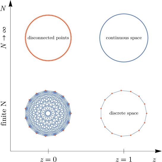
Figure 1: Pictorial representation of the phases of connectivity as a function of the anisotropic scaling $z$ and the number of nodes $N$. For finite $N$, the exemplary ring graph (bottom right) at $z=1$ transforms into complete graph (bottom left) in the ultralocal limit ($z\rightarrow 0$). In the continuous ($N\rightarrow\infty$) limit the ring graph reduces to a circle (top right) and the complete graph transfigures into a set of disconnected points (top left).

For finite $N$, the ring graph at $z=1$ transitions into a complete graph in the ultralocal limit $z\rightarrow 0$). While performing the continuous ($N\rightarrow\infty$) limit the graph at $z=1$ reduces to a circle ($S^{1}$) and a complete graph at $z=0$ reduces to a set of disconnected points. The later behavior is due to the weights $w=\frac{1}{N}$ associated with the links in the ultralocal limit. Worth mentioning here is that the three configurations: discrete space, disconnected points and the crumpled state have also been observed to occur together in the Quantum Graphity approach [17].

The connected graph (at $z=0$ and finite $N$) represents a crumpled phase, in particular similar to the one observed in CDT. To make the relation with CDT closer one can view the considered graphs as graph of nodes of triangulations in CDT. The observations made above suggest that the $B$ phase of CDT (observed for both spherical [18] and toroidal [19] topologies) reflects the ultralocal state of gravity. Because in the CDT simulations, a finite number of simplices ($N$) is considered the phase manifests as the crumpled state.

One of the consequences of the observation made here is that puzzling divergence of the spectral dimension in the ultralocal limit predicted by Horava-Lifshitz theory can now be understood. This issue is addressed in Sec. 4.

3 The ring graph model

Results of the previous section are general and are not dependent on dimensionality of the universe (graph) in the $z=1$ limit. However, it would be difficult to analyze further properties of the geometrogenesis without making assumptions about the relational structure in the geometric limit. The case which allows for a broad analytical analysis is the $S^{1}$ geometry, which in discrete version is described by a ring graph. Therefore, in our further investigations we will focus on a model in which the $z=1$ limit is described by a ring graph composed of $N$ nodes. One can perceive this case as a prototype low-dimensional model of a spatially compact universes.

The ring graph is invariant under cyclic permutation of indices $i\rightarrow i+1$, associated with the $\mathbb{Z}_{N}$ group. The symmetry is generated by the group element $g$, which commutes with the Laplace operator $\Delta$. Because of this, $\Delta$ and $g$ have the common set of eigenvectors. Using the fact that $g^{N}=\mathbb{I}$, together with the eigenequation $ge_{n}=g_{n}e_{n}$ one can show that the eigenvalues $g_{n}$ correspond to the complex roots of the equation $g_{n}^{N}=1$, which are $g_{n}=e^{i2\pi(n-1)/N}$ and $n=1,2,\dots,N$. Now, with the use of the action of the group element $g$ on the eigenvectors $g(e_{n})_{j}=(e_{n})_{j+1}$, functional form of the normalized eigenvectors can be found:

$$(e_{n})_{j}=\frac{1}{\sqrt{N}}e^{i2\pi(n-1)j/N},$$ (14)

which are normalized using $\sum_{j=1}^{N}(e_{n})_{j}(e_{m}^{*})_{j}=\delta_{nm}$. Applying the derived eigenfunctions to the eigenequation $\Delta e_{n}=\lambda_{n}e_{n}$, the eigenvalues of the Laplace operator $\Delta$ can be determined:

$$\lambda_{n}=2\left[1-\cos\left(2\pi\frac{(n-1)}{N}\right)\right],$$ (15)

where $n=1,2,\dots,N$. The eigenvalues applied to Eq. 7 allow us to determine eigenvalues of the $\Delta_{z}$ Laplace operator, which are elements of the diagonal matrix:

$$\Lambda^{z}={\rm diag}(\lambda_{1}^{z},\lambda_{2}^{z},\dots,\lambda_{N}^{z}),$$ (16)

where $\lambda_{n}$ are given by Eq. 15. In consequence, one write eigenvalues of the $\Delta_{z}$ Laplace operator as:

$$\lambda^{z}_{n}=2^{z}\left[1-\cos\left(2\pi\frac{(n-1)}{N}\right)\right]^{z},$$ (17)

where $n=1,2,\dots,N$. Furthermore, because $\Delta_{z}=P\Lambda^{z}P^{\dagger}$ and the $P$ matrices can be expressed in terms of the eigenfunctions (14) the matrix elements of $\Delta_{z}$ can be written as follows:

$$\left(\Delta_{z}\right)_{mn} =P_{mk}\Lambda_{kl}^{z}P_{ln}^{\dagger}=\sum_{k=1}^{N}\sum_{l=1}^{N}(e_{k})_{m}\delta_{kl}\lambda^{z}_{k}(e^{*}_{l})_{n}=\frac{1}{N}\sum_{k=1}^{N}e^{i2\pi(k-1)(m-n)/N}\lambda^{z}_{k}$$

$$=\frac{1}{N}\sum_{k=1}^{N}e^{i2\pi(k-1)(m-n)/N}2^{z}\left[1-\cos\left(2\pi\frac{(k-1)}{N}\right)\right]^{z}.$$ (18)

Furthermore, the $\Delta_{z}$ is a real matrix (proof can be found in A). Therefore, the imaginary component of Eq. (18) must vanish and we can write that

$$\left(\Delta_{z}\right)_{mn}=\frac{1}{N}\sum_{k=1}^{N}\cos\left[2\pi(k-1)(m-n)/N\right]2^{z}\left[1-\cos\left(2\pi\frac{(k-1)}{N}\right)\right]^{z}.$$ (19)

It is straightforward to show that the ultralocal limit (9) is correctly recovered from this expression. The valence of a $n$-th node is now easy to determine from:

$$d_{n}:=\left(\Delta_{z}\right)_{nn}=\frac{2^{z}}{N}\sum_{k=1}^{N}\left[1-\cos\left(2\pi\frac{(k-1)}{N}\right)\right]^{z}.$$ (20)

In particular, in the ultralocal limit ($z\rightarrow 0$) we obtain

$$\lim_{z\rightarrow 0}d_{n}=\frac{1}{N}\sum_{k=2}^{N}1=\frac{1}{N}(N-1),$$ (21)

in accordance with Eq. 11. The $1/N$ factor corresponds to the weight $w$ associated with the links and the $N-1$ factor counts the number of links attached to any node.

It is interesting to observe that, the thermodynamic limit ($N\rightarrow\infty$) of the expression (20) can be performed by introducing the angle variable $\theta:=2\pi\frac{(k-1)}{N}$. This allows us to write:

$$d_{n}^{N\rightarrow\infty}:=\lim_{N\rightarrow\infty}d_{n}=\frac{2^{z}}{2\pi}\int_{0}^{2\pi}(1-\cos{\theta})^{z}d\theta=\frac{4^{z}\Gamma\left(z+\frac{1}{2}\right)}{\sqrt{\pi}\Gamma(z+1)}<\infty,$$ (22)

for $z\in[0,1]$, where $\Gamma(x)$ is the gamma function. In Fig. 2 we plot behavior of the effective degree of nodes given by Eq. 20 and Eq. 22.

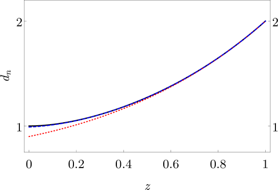
Figure 2: Effective degree of nodes $d_{n}$ as a function of $z$. The (black) continuous curve corresponds to the $N\rightarrow\infty$ case given by Eq. 22. The (red) dotted curve plotted for $N=10$ and the (blue) dashed curve corresponds to $N=100$ and overlaps with the curve for $N\rightarrow\infty$.

The value of $2$ is correctly recovered in for $z=1$. On the other hand, in the ultralocal limit ($z\rightarrow 0$) the value of $d_{n}$ converges to $d_{n}=1$ as expected based on Eq. 21 taken in the $N\rightarrow\infty$ limit.

4 Spectral dimension

In the recent years the so-called spectral dimension attracted significant attention in analyzes of different quantum gravitational space(time) configurations. The studies concerned such approaches to quantum gravity and models of the Planck scale physics as Causal Dynamical Triangulations [20], Loop Quantum Gravity [21], Multifractal theories [22], Asymptotic Safety [23], Causal Sets [24], Deformed Poincaré algebras [25], etc.

The spectral dimension is defined with the use of diffusion process performed in some external time $\sigma$. The idea behind the definition of the spectral dimension is based on the diffusion time dependence of the average return probability $P(\sigma)$ which can be determined as a trace of the Heat Kernel $K({\bf x},\tau,{\bf x}^{\prime},\tau^{\prime};\sigma)$.

In the considered case of the anisotropic scaling (2), employing the appropriate spatial Laplace operator (3), the heat kernel equation takes the following form [15]:

$$\frac{\partial}{\partial\sigma}K({\bf x},\tau,{\bf x}^{\prime},\tau^{\prime};\sigma)=\left(\frac{\partial^{2}}{\partial\tau^{2}}-\Delta_{z}\right)K({\bf x},\tau,{\bf x}^{\prime},\tau^{\prime};\sigma),$$ (23)

here $\tau=-it$ is the Wick rotated coordinate time $t$. Continuous solution to (23) can be found and the corresponding value of the spectral dimension can be determined [15]:

$$d_{S}:=-2\frac{d\log P(\sigma)}{d\log\sigma}=1+\frac{d}{z},$$ (24)

where $d$ is the spatial topological dimension of the spatial part.

In case of GR ($z=1$), the spectral dimension (24) reduces to the space-time dimension $d_{S}=1+d$. However, in the relevant ultralocal limit $z\rightarrow 0$, the spectral dimension tends to infinity, $d_{S}\rightarrow\infty$. As we will show below, such behavior is expected for the complete graph describing the ultralocal phase for a finite $N$.

For our purposes it is relevant to consider diffusion without the time dimension, which can be easily added to the final results. Then, for the matrix Laplace operator $\Delta_{z}$ the solution to the Heat Kernel equation can be expressed in terms of eigenvectors $e_{n}$ and eigenvalues $\lambda^{z}_{n}$ of the operator. Straightforward analysis leads to the following expression:

$$K(i,j;\sigma)=\sum_{n=1}^{N}e^{-\lambda^{z}_{n}\sigma}(e_{n})_{i}(e^{*}_{n})_{j},$$ (25)

which allows to derive expression of the average return probability

$$P(\sigma):={\rm tr}K(i,j;\sigma)=\sum_{n=1}^{N}e^{-\lambda^{z}_{n}\sigma}.$$ (26)

Based on the above expression the spectral dimension can be written as follows:

$$d_{S}=2\sigma\frac{\sum_{n=1}^{N}\lambda^{z}_{n}e^{-\lambda^{z}_{n}\sigma}}{\sum_{n=1}^{N}e^{-\lambda^{z}_{n}\sigma}}.$$ (27)

In Fig. 3 we plot Eq. 27 as a function of both diffusion time $\sigma$ and the anisotropic scaling parameter $z$ for a ring graph with $N=100$.

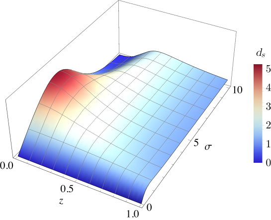
Figure 3: Spectral dimension as a function of diffusion time $\sigma$ and the anisotropic scaling parameter $z$ for a ring graph with $N=100$. For $z=1$ the spectral dimension saturates $d_{S}=1$ as expected for the ring graph. In the ultralocal limit, the spectral dimension is peaked at some $\sigma_{*}\sim 1/N$ and falls to zero for $\sigma\rightarrow\infty$.

In the case of a complete graph which corresponds to the $z\rightarrow 0$ phase the besides the zero eigenvalue $\lambda_{1}=0$ all remaining eigenvalues are equal and given by $\lambda_{2}=\lambda_{3}=\dots=\lambda_{N}=1$. In consequence, the analytic expression for the spectral dimension is [12]

$$d_{S}=\frac{2\sigma(N-1)}{e^{\sigma}+(N-1)}.$$ (28)

The spectral dimension peaks at some $\sigma_{*}\sim 1/N$ and falls to zero for $\sigma\rightarrow\infty$. In the continuous ($N\rightarrow\infty$) limit $d_{S}\rightarrow\infty$ at $\sigma=0$ and is equal zero elsewhere. The divergence of the spectral dimension in the ultralocal limit is therefore a residue of the high connectivity of the crumpled phase. Namely, at small diffusion times there is a huge number of possible nodes to go, such that the corresponding dimensionality is perceived to be very high.

5 Ising matter and phase transitions

So far we have been focused solely on properties of the graph representing connectivity structure of space(time). The easiest way to go beyond this level and to introduce some local degrees of freedom is by assigning classical spins $s_{i}\in\{-1,1\}$ to every node. Such degrees of freedom can either be consider as a prototype of gravitational degrees of freedom or as a matter sector. The simplest nontrivial Hamiltonian for the spins is

$$E=-\frac{1}{2}\sum_{i,j}w_{ij}s_{i}s_{j}-h\sum_{i}s_{i},$$ (29)

where $w_{ij}$ are the weights associated with given links and $h$ is some external bias.

The case of $z=0$ for which $w_{ij}=\frac{1}{N}(1-\delta_{ij})$, is especially worth considering here and leads to

$$E=-\frac{1}{2N}\sum_{i\neq j}s_{i}s_{j}-h\sum_{i}s_{i},$$ (30)

the well known Curie-Weiss model. The weights introduce the $1/N$ factor in a natural way which correctly ensures existence of the thermodynamic limit. The corresponding statistical model can be solved analytically with the use of following observation

$$\left(\sum_{i}s_{i}\right)^{2}=N+\sum_{i\neq j}s_{i}s_{j},$$ (31)

and by applying the Hubbard-Stratanovich transformation. Finally, one gets an equation of state for magnetization which predicts existence of a second order phase transition. For $z=1$ the phase properties depend on the effective dimensionality of the graph. In particular, in the one dimensional case (ring graph) no phase transition is expected while in the higher dimensional cases second order phase transitions are known to occur. Hence, we pose an interesting question - do phase transitions occur on the whole $z=[0,1)$ interval? In what follows, for simplicity, we consider the case with $h=0$.

5.1 Analytical results

To answer this question we first go back to our $z$-dependent Laplacian $\Delta_{z}$ based on the ring graph and determine the coupling $J(n)$ between the spin at distance $n$. With the use of Eq. 19 we define

$$J(n):=w_{1,n+1}=-(\Delta^{z})_{1,n+1}=-\frac{2^{z}}{N}\sum_{k=1}^{N}\cos\left[2\pi\frac{(k-1)n}{N}\right]\left[1-\cos\left(2\pi\frac{(k-1)}{N}\right)\right]^{z}.$$ (32)

The important property, of this function resulting from the symmetry of the ring graph is that $J(i)=J(N-i)$ for all $i$. In Fig. 4 we plot Eq. 32 as a function of $z$ for a ring graph with $N=100$.

Figure 4: Exemplary couplings $J(n)$ as a function of the anisotropic scaling parameter $z$ for a ring graph with $N=100$. The solid curve corresponds to $J(1)$, dashed to $J(2)$ and dotted to $J(3)$.

For $z=1$, only $J(1)$ contributes as expected for the nearest neighbor Ising model. On the other hand, in the ultralocal limit ($z\rightarrow 0$) all couplings have the same value $J(n)=w=\frac{1}{N}$, in agreement with Eq. 10. In the thermodynamical limit ($N\rightarrow\infty$) the expression for $J(n)$ can be written as

$$J(n)=-\frac{2^{z}}{2\pi}\int_{0}^{2\pi}(1-\cos{\theta})^{z}\cos(\theta n)d\theta=\frac{(-1)^{n}\Gamma(n-z)\sin(\pi(n-z))}{\sin(2\pi z)\Gamma(-2z)\Gamma(1+n+z)}.$$ (33)

One can notice that the interaction $J(n)$ disappears as $n\rightarrow\infty$ for $\forall z$. Thus, graph vertices distributed far away do not interact. In Fig. 5 we graphically compare $J(1)$ and $J(10)$ obtained with the use of formula (33) with the corresponding finite $N$ results for $N=100$. As expected, the values of $J(n)$ at $z=0$ tend to zero in the thermodynamic limit for $\forall n$.

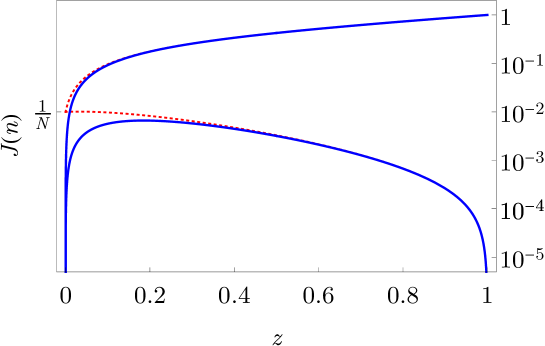
Figure 5: Exemplary thermodynamical limits of $J(n)$ for $n=1$ (top curve) and $n=10$ (bottom curve) plotted as a function of $z$. The dotted curves represent corresponding expression for $J(n)$ for finite $N=100$.

The purpose of investigating $J(n)$ was that the existence of phase transitions is guaranteed by fulfillment of the two following conditions [26]:

1. The total interaction between vertex and all of its neighbors is bounded, i.e.

   $$M_{0}=\sum_{n=1}^{\infty}J(n)<\infty.$$ (34)

2. The sum of interactions multiplied by their distance $n$ should be unbounded, i.e.

   $$M_{1}=\sum_{n=1}^{\infty}nJ(n)=\infty.$$ (35)

The condition (i) is satisfied automatically given that double of graph interaction in one direction is always given by the previously found vertex degree. We verify this fact with simple calculation performed in the thermodynamic limit:

$$\begin{split}2M_{0}&=2\sum_{n=1}^{\infty}J(n)=2\sum_{n=1}^{\infty}\frac{(-1)^{n}\Gamma\left(n-z\right)\sin{\pi(n-z)}}{\sin(2\pi z)\Gamma(-2z)\Gamma(1+n+z)}\\ &=-\frac{\Gamma(1-z)}{2z\cos(\pi z)\Gamma(-2z)\Gamma(1+z)}=\frac{4^{z}\Gamma\left(z+\frac{1}{2}\right)}{\sqrt{\pi}\Gamma(z+1)}.\end{split}$$ (36)

The second (ii) condition, first derived by Ruelle [27] for spins arranged on infinite line, must be modified to account for the ring topology. The physical motivation behind this condition and its modification is simple yet intriguing, however in order to keep our reasoning short and clear we defer it to B. The modification of Ruelle’s condition results in:

$$M_{1}=a_{1}+\sum_{m=1}^{N/2}b_{m},$$ (37)

where

$$b_{m}=\frac{2^{2z}}{N}\left[\sin\left(\pi\frac{2m-1}{N}\right)\right]^{2(z-1)}.$$ (38)

The convergence properties (when $N\rightarrow\infty$) of the above sum can be evaluated in the continuous thermodynamical limit which can be written as

$$M_{1}=\delta(z)+\frac{2^{z}}{2\pi}\int_{0}^{\pi}d\theta(\sin\theta)^{2(z-1)}=\left\{\begin{array}[]{cc}\infty&\text{for}\ z\in[0,1/2]\\ \frac{2^{z}}{2\sqrt{\pi}}\frac{\Gamma(-1/2+z)}{\Gamma(z)}&\text{for}\ z\in(1/2,1]\end{array}\right..$$ (39)

This equation indicates that a phase transition can occur at $z\in[0,1/2]$. One might ask what happens with the critical temperatures in this critical segment. In the next section we show that, with limited success (partly because of finite-size effects described in B.2) this question can be answered through numerical simulations.

5.2 Numerical results

Numerical simulations of the system under consideration were performed using regular Monte Carlo techniques. For any choice of $z=[0,1]$, number of spins $N$ and inverse temperature $\beta:=1/T$ the system was properly thermalized and certain observables were computed. Averaging $\langle\dots\rangle$ of quantities in question was performed over equilibrium configurations. In particular, we have focused our analysis on computing the magnetization

$$s=\frac{1}{N}\sum_{i=1}^{N}s_{i},$$ (40)

based on which, values of averaged magnetization

$$\mathcal{M}=\langle s\rangle,$$ (41)

and Binder cumulant

$$\mathcal{B}=1-\frac{\langle s^{4}\rangle}{3\langle s^{2}\rangle^{2}}.$$ (42)

were determined. Exemplary plots are shown in Fig. 6. Properties of the Binder parameter imply $\mathcal{B}\rightarrow 2/3\approx 0.667$ in the symmetry broken phase and $\mathcal{B}\rightarrow 0$ in the symmetric phase. Furthermore, at the critical point $0<\mathcal{B}<2/3$.

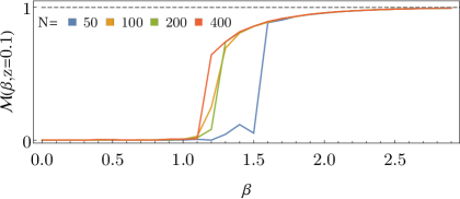
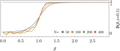
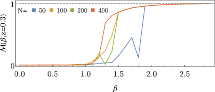
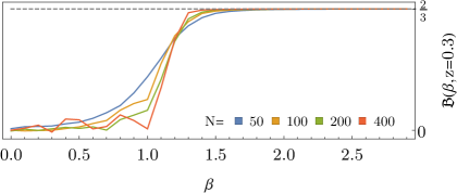
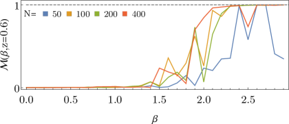
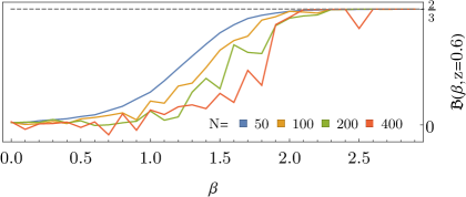
Figure 6: Columns - average magnetization $\mathcal{M}$ and Binder parameter $\mathcal{B}$ as a function of inverse temperature $\beta$ for different values of $z$ (rows).

In accordance with the analytical consideration, in the ultralocal limit ($z\rightarrow 0$) the Curie-Weiss critical point has been identified. In the normalized units, location of the critical point is consistent with the theoretically predicted value $\beta_{\text{C}W}=1$ or $T_{\text{C}W}=1$. Together with the increase of $z$ the location of the critical point shifts to the smaller temperatures (higher values of $\beta$). However, while the value of $z=0.5$ is approached, fluctuations are becoming dominant and analysis of the Binder cumulant does not support existence of the symmetry broken phase for $z>0.5$. This is is accordance with the results of analytical investigations performed in the previous subsection. Furthermore, for small values of spin chain size ($N$) finite-size effects discussed in the previous subsection skew the results, whereas for large values $N$, the equilibrium state was difficult to obtain near the disappearing ($z>1/2$) phase transitions. Based on the joint numerical and analytical studies the expected phase space of the system has been sketched in Fig. 7.

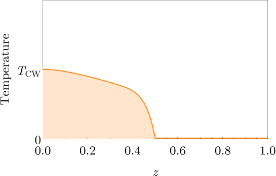
Figure 7: Phase diagram of the considered spin system at the Temperature-$z$ plane. The $T_{CW}$ corresponds to critical temperature of Curie-Weiss model. The critical point extends to a critical line which ends at $z=0.5$. The shadowed region corresponds to the symmetry broken phase. In the remaining part of the phase diagram the system is in symmetric phase.

One can conclude that for $z\in[0,0.5)$ there exist symmetry broken phase at temperatures $T>0$. The associated critical line matches with the Curie-Weiss critical point at $z=0$. Furthermore at $z\in[0.5,1]$ only the symmetric phase exists. The result is in accordance with the known behavior of the nearest neighbor Ising model on $S^{1}$, which is realized at $z=1$. Worth stressing is that the presented model provides interesting interpolation between the two analytical spin systems, one with and second without critical behavior. Therefore, the presented model may possibly have relevance outside of the considered here gravitational context. More robust analysis, including its quantum counterpart and $h\neq 0$ case is beyond the scope of this article and will be pursued in the forthcoming papers.

6 Cosmological implications

In this section we are going to discussion potential cosmological significance of the process of geometrogenesis discussed in this article, which would be associated with transition in time from $z=0$ to $z=1$.

Let us begin with emphasizing that one of the most important properties of the state of the early universe is its nearly scale-invariant nature of cosmological inhomogeneities, reflected in the anisotropy of the Cosmic Microwave Background (CMB) radiation. A perfect scale-invariance would mean that the connected two-point correlation is invariant under rescaling ${\bf x}\rightarrow b{\bf x}$:

$$\langle\phi({\bf x})\phi({\bf y})\rangle_{c}=\langle\phi(b{\bf x})\phi(b{\bf y})\rangle_{c},$$ (43)

which means that the correlator is a constant function of the distance $r:=|{\bf x}-{\bf y}|$. The two-point function can be expressed in terms of the so-called power-spectrum $\mathcal{P}(k)$ in the following way:

$$\langle\phi({\bf x})\phi({\bf y})\rangle_{c}=\int_{0}^{\infty}\frac{dk}{k}\mathcal{P}(k)\frac{\sin(kr)}{kr}.$$ (44)

A simple analysis implies that scale-invariance leads to the constant power spectrum $\mathcal{P}(k)=$ const., which is called the Harrison-Zeldovich power spectrum. The departure from the scale invariance is parametrized by the spectral index $n$, such that $\mathcal{P}(k)\propto k^{n-1}$. The most up to date observations of the scalar perturbations indicated that $n_{S}=0.9616\pm 0.0094$ [28].

In the crumpled phase ($z\rightarrow 0$) represented by the connected graph the two point correlation function $\langle s_{i}s_{j}\rangle_{c}=\langle s_{i}s_{j}\rangle-\langle s_{i}\rangle\langle s_{j}\rangle$ does not depend on the values of $i$ and $j$ since all spins are treated at equal footing. The two point correlation function, therefore, does not depend on the distance between given points $i$ and $j$ (all distances are equal) but only on parameters of the model and temperature. However, due the effective change of dimensionality, we cannot directly conclude if the fluctuations in the ultralocal state ($z\rightarrow 0$) are scale invariant. However, some investigations suggest that critical behavior associated with geometrogenesis may lead to nearly scale-invariant powers spectrum of primordial perrurbations [29].

More detailed analysis of the vacuum quantum fluctuations employees the following mode equation [30]

$$\frac{d}{d\eta^{2}}f_{k}+\left(k^{2z}-\frac{z_{i}^{\prime\prime}}{z_{i}}\right)f_{k}=0,$$ (45)

where $\eta$ is the conformal time and the $\Delta_{z}$ Laplace operator (3) has been taken into account. The form of $z_{i}$ depends on whether tensor $i=T$ or scalar $i=S$ perturbations are considered. With the use of Bunch-Davies type of vacuum normalization, the vacuum power spectrum can be expressed as

$$\mathcal{P}(k):=\frac{k^{3}}{2\pi^{2}}\left|\frac{f_{k}}{z_{i}}\right|^{2}=\frac{k^{3}}{2\pi^{2}}\frac{1}{2\omega}\frac{1}{z_{i}^{2}},$$ (46)

where dependence of the $\omega$ on $k$ is given be an appropriate dispersion relation. In the case considered in this article, the modified spatial part of the Laplace operator (3) implies that $\omega^{2}=k^{2z}$. This leads to the expression $\mathcal{P}(k)\propto k^{3-z}$, such that the scale-invariance is recovered at the Lifshitz point ($z=3$). In turn, the ultralocal limit leads to the cubic power spectrum $\mathcal{P}(k)\propto k^{3}$ describing white noise type of fluctuations for which the two-point correlation function is just vanishing:

$$\langle\phi({\bf x})\phi({\bf y})\rangle_{c}=0.$$ (47)

This is in agreement with the the analysis of the ultralocal state performed in the context of loop quantum cosmology [31]. Moreover, worth mentioning is that the white noise power spectrum is also scale-invariant, though, in a trivial way since the correlation function is just equal zero.

The possibility interesting from the cosmological perspective is the transition across the second-order transition occurring in the setup discussed in the previous section. Since such transition is hypothesized to occur in a finite amount of time, formation of domains as well as associated topological defects are expected. The process is described by the so-called Kibble-Zurek [32, 33] mechanism which takes into account scaling of both correlation length:

$$\xi=\xi_{0}\left|1-T/T_{C}\right|^{-\nu},$$ (48)

and the relaxation time

$$\tau=\tau_{0}\left|1-T/T_{C}\right|^{-\nu Z},$$ (49)

where $\nu$ and $Z$ are critical exponents characterizing the equilibrium version of the considered phase transition. Based on this, the diameter of the relaxation horizon can be expressed as follows:

$$\xi_{c}=\int_{0}^{t}\frac{\xi(T)}{\tau(T)}dt\propto\xi_{0}\frac{\tau_{Q}}{\tau_{0}}\left(1-T/T_{C}\right)^{\nu(Z-1)+1},$$ (50)

where we introduced the so-called quench time $\tau_{Q}$ which characterizes a speed of the transition. The process of relaxation will stop when the size of the relaxation horizon becomes equal with the correlation length $\xi_{c}(T_{F})=\xi(T_{F})$. This condition leads to the following expression for the domain size:

$$\xi\approx\xi_{0}\left(\frac{\tau_{Q}}{\tau_{0}}\right)^{\frac{\nu}{\nu Z+1}}.$$ (51)

The topological defects are formed at the boundaries between the domains. For typical values of the parameters we obtain $\xi\approx l_{\rm Pl}$. Assuming that there is no inflation the rough estimation of the density of defects is:

$$n\sim\frac{1}{\xi^{3}}\left(\frac{T_{\rm CMB}}{T_{\rm Pl}}\right)^{3}\sim 1\frac{\text{defect}}{\text{mm}^{3}}.$$ (52)

If the phase of inflation occurs after the second order phase transition, the value of $n$ can be further diluted with the $e^{-3N}$ factor, where $N$ is the number of inflationary $e$-folds. This number is expected to not be less that $N\sim 60$. In consequence, the expected present number of defects is suppresses by at least the enormous $10^{-180}$ factor, which makes any current empirical relevance of the defects groundless.

7 Summary and discussion

The main purpose of this article was to investigate interconnection between the phase of ultralocality and the process of geometrogenesis. The studies were inspired by the observation made in Ref. [13] which suggested that the ultralocality shares some features of the crumpled state of gravitational field characterized by enormous level of connectivity.

In our studies, the anisotropic scaling introduced in the context of Horava-Lifshitz theory has been considered. In such a case, the ultralocal limit is recovered by taking the $z\rightarrow 0$ limit, while the standard relativistic scaling is satisfied at $z=1$. By analyzing the properties of the Laplace operator, connectivity structure in the $z\rightarrow 0$ has been reconstructed. We proved analytically than in the $z\rightarrow 0$ limit the spatial connectivity is represented by a complete graph. However, such relation is satisfied for finite system only. We have shown that when the number of nodes $N$ grows to infinity, the complete graph disintegrates into a set of points. This observation supports the discussion of Ref. [35], which stressed the dependence of the semiclassical limit on the number of degrees of freedom. In our case, we observed that depending on whether finite or infinite number of nodes is considered, the corresponding phase may have qualitatively different properties.

Furthermore, we have shown that the transition between the ultralocal state and the geometric state of gravity can be associated with the process of removing links from the graph representing connectivity structure between the points of space. The process can describe hypothetical geometrogenesis occurring in the early universe. In such a picture, the evolving (maturing) Universe drastically reduces number of spatial interconnections. Worth mentioning is that there are also other complex systems observed in Nature, which exhibit such reduction of connectivity. One of the seminal examples of such a behavior is the so-called synaptic pruning occurring in the maturing brain [34]. While newborn brain is full of connections, its maturing reduces relative number of connections with respect to the number of neurons (nodes of a graph). Such reduction is associated with both optimization of the brain functioning and the process of learning. From such a perspective one can hypothesize that the maturing universe removes some irrelevant connection in its structure. In consequence, the connectivity structure (encoded in the weights $w_{ij}$) undergoes specialization in similarity with the process of learning.

In order to study a potential critical behavior associated with the geometrogenesis we have introduced Ising type matter defined at the nodes of the considered graph. Both analytical and numerical studies of the system were performed for $z\in[0,1]$, with the analysis limited to the special case of a ring graph ($S^{1}$ topology) at $z=1$. As we have shown, the Curie-Weiss critical point is recovered at $z=0$ and extends as a critical line in the $z\in[0,0.5)$ range. The second order nature of the transition line has been confirmed by the numerical investigations of the Binder cumulant. We have shown that the symmetry broken phase does not occur in the $z\in(0.5,1]$ range.

Finally, some possible cosmological consequences of the considered scenario were investigated. In particular, we have confirmed, that the ultralocal limit is associated with the white noise type of fluctuations. Furthermore, we have stressed that the identified critical line may lead to the formation of domains and topological defects. Observational constraints on the number of topological defects may allow one to put some constraints on the discussed features in early universe.

Appendix A Proof of real-valuedness of $\Delta_{z}$

This property can be formally proven with the following calculation:

$$\Im\left[\left(\Delta_{z}\right)_{mn}\right]=\frac{1}{N}\sum_{k=1}^{N}\sin\left[2\pi(k-1)(m-n)/N\right]2^{z}\left[1-\cos\left(2\pi\frac{(k-1)}{N}\right)\right]^{z}$$

$$=\sum_{r=0}^{\infty}(-1)^{r}\left(\begin{array}[]{c}z\\ r\end{array}\right)\frac{2^{z}}{N}\sum_{k=1}^{N}\sin\left[2\pi(k-1)(m-n)/N\right]\cos^{r}\left[2\pi(k-1)/N\right],$$ (55)

which followed by the Fourier decomposition,

$$\cos^{r}\left[2\pi(k-1)/N\right]=\sum_{l=1}^{N}c_{l}\cos\left[2\pi(k-1)l/N\right]$$ (56)

together with the orthogonality relation

$$\sum_{k=1}^{N}\sin\left[2\pi(k-1)m/N\right]\cos\left[2\pi(k-1)n/N\right]=0,$$ (57)

completes the proof that $\Im\left[\left(\Delta_{z}\right)_{mn}\right]=0$.

Appendix B Intuition behind Ruelle’s condition and it’s modification

The physical motivation behind Ruelle’s condition is that energy of interaction between two infinite domains of $\dots+++++++\dots$ and $\dots-------\dots$ orientations of spins must be infinite to withstand thermal fluctuations that could spoil stability of a given phase. In the case of the Ising model on $\mathbb{R}$ there is only a single boundary between the domains. And there is a single contribution to the interaction from $J(1)$, there are two pairs which interact with $J(2)$, three pairs which interact with $J(3)$, etc. leading to the expression (35). In the considered case of $S^{1}$ topology of the graph for $z=1$, instead of a single boundary there are two boundaries between the domains, which have to be taken into account while calculating the energy of interactions between the domains. Before, we study the general case let us calculate first the energy of interaction between the domains for $z=0$ and $z=1$. For $z=0$ there is a Curie-Weiss phase transition, so we expect that $M_{1}=\infty$, on the other hand there is no phase transition for $z=1$ in the case of considered ring graph, and in consequence $M_{1}<\infty$. Let us suppose that we have two domains each containing $N/2$ Ising spins. Then there are $\sim\left(\frac{N}{2}\right)^{2}$ links between the two domains each associated with the same coupling $J(n)=\frac{1}{N}$. In consequence, the energy of interaction between the two domains is $M_{1}=\left(\frac{N}{2}\right)^{2}\frac{1}{N}\sim N$, which is infinite in the thermodynamical limit ($N\rightarrow\infty$). On the other hand at $z=1$ only $J(1)$ contributes and energy of interaction between the two domains is just $2J(1)=2$, which is finite even in the thermodynamic limit.

Assuming that $N$ is even, the interaction energy between the two domains (each of the $N/2$ size) defined at the ring graph can be calculated as follows. Let us suppose that $i=1,2,\dots,N/2$ are ”+” spins and $i=N/2,N/2+1,\dots,N$ are ”-”, the interaction energy between the $i$-th positive spin and all spins from the domain of negative spins is:

$$E_{i}=\sum_{n=N/2}^{N-1}J(n-(i-1)).$$ (58)

Based on this, $M_{1}$ can calculated by summing up $E_{i}$ over all of the spins belonging to the domains of the positive spins, i.e.

$$M_{1}=\sum_{i=1}^{N/2}\sum_{n=N/2}^{N-1}J(n-(i-1))=\sum_{k=1}^{N}a_{k},$$ (59)

where

$$a_{1}=-2^{2(z-1)}N\lim_{k\rightarrow 1}\left[\sin\left(\pi\frac{k-1}{N}\right)\right]^{2z},$$ (60)

and for $k>1$

$$a_{k}=\frac{2^{2(z-1)}}{N}\left(1-(-1)^{k-1}\right))^{2}\left[\sin\left(\pi\frac{k-1}{N}\right)\right]^{2(z-1)}.$$ (61)

In Fig. 8 we plot $M_{1}$ as a function of $z$ for the $N=20$. As expected, the function converges to $M_{1}=2$ for $z=1$ and is equal to $\left(\frac{N}{2}\right)^{2}\frac{1}{N}=\frac{N}{4}$ in the ultralocal limit.

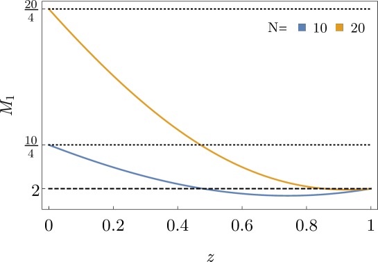
Figure 8: Values of function $M_{1}(z)$ for finite-size ($N$) spin chains. The curves correctly match with $M_{1}=N/4$ at $z=0$ and $M_{1}=2$ at $z=1$.

In order to verify what is the behavior of $M_{1}$ for $N\rightarrow\infty$, we can study convergence property for the sum $M_{1}(N,z)$ which can be further simplified to

$$M_{1}=a_{1}+\sum_{m=1}^{N/2}b_{m},$$ (62)

where

$$b_{m}=\frac{2^{2z}}{N}\left[\sin\left(\pi\frac{2m-1}{N}\right)\right]^{2(z-1)}.$$ (63)

B.1 Alternative method of calculating Ruelle’s condition

Simultaneously, another interesting insight can be given. One could argue that in the thermodynamic limit the expression (33) has lost the information about the ring topology ($J(N/2-1)\neq J(N/2+1)$) and that one could “recover” the right behavior by calculating $M_{1}$ as

$$\lim_{N\rightarrow\infty}\sum_{n=1}^{N}nJ(n/2),$$ (64)

which in fact gives the same result as (39), even though the input for $J$ was assumed to be an integer.

B.2 Finite size effects

Skimming through the presented analysis one might get the idea that numerical simulations of the presented spin system might be a viable option. This presumption however, is true only for large spin systems (assuming we can simulate such) and $z<1/2$, in rest of the cases we can predict finite-size effects simply due to ring topology. One can see this most clearly by working through the sum (59):

$$\begin{split}&\sum_{i=1}^{N/2}\sum_{n=N/2}^{N-1}J(n-(i-1))=\sum_{i=1}^{N/2}\sum_{n=1}^{N/2}J\left(-(i-1)+n+N/2-1\right)\\ &\overset{n-i=k}{=}\sum_{k=1}^{N/2}2\left(\frac{N}{2}-k\right)J\left(\frac{N}{2}-k\right)+\frac{N}{2}J\left(\frac{N}{2}\right)=\sum_{u=1}^{N/2-1}2uJ(u)+\frac{N}{2}J\left(\frac{N}{2}\right)\end{split}.$$ (65)

The second term of the last expression holds the information about the interaction of each spin with its partner from the opposite side of the ring. It can be shown that this term vanishes in the thermodynamic limit, however it is worthwhile to look at its dependence on $N$ (Fig. 9), to notice the mentioned finite-size effects, strongest near $z\approx 1$. Nevertheless, numerical results can provide us some qualitative information about the transitions of the critical temperatures.

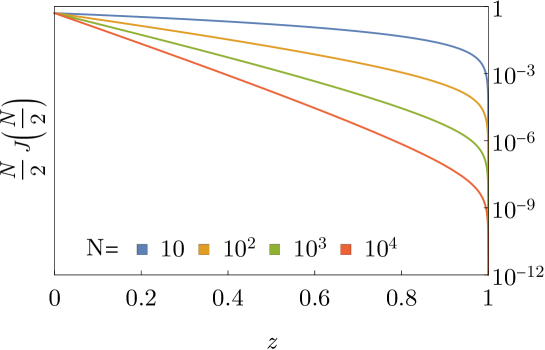
Figure 9: Contribution of the far-away interaction to $M_{1}(z)$.

References

References

- [1] V. A. Belinsky, I. M. Khalatnikov and E. M. Lifshitz, Adv. Phys. 19 (1970) 525. doi:10.1080/00018737000101171
- [2] V. a. Belinsky, I. m. Khalatnikov and E. m. Lifshitz, Adv. Phys. 31 (1982) 639. doi:10.1080/00018738200101428
- [3] L. Andersson, H. van Elst, W. C. Lim and C. Uggla, Phys. Rev. Lett. 94 (2005) 051101 doi:10.1103/PhysRevLett.94.051101 [gr-qc/0402051].
- [4] J. Mielczarek, AIP Conf. Proc. 1514 (2012) 81 [arXiv:1212.3527 [gr-qc]].
- [5] M. Bojowald and G. M. Paily, Phys. Rev. D 87 (2013) no.4, 044044 [arXiv:1212.4773 [gr-qc]].
- [6] A. Eichhorn, S. Mizera and S. Surya, Class. Quant. Grav. 34 (2017) no.16, 16LT01 [arXiv:1703.08454 [gr-qc]].
- [7] P. Horava, Phys. Rev. D 79 (2009) 084008 [arXiv:0901.3775 [hep-th]].
- [8] J. Ambjorn, S. Jordan, J. Jurkiewicz and R. Loll, Phys. Rev. D 85 (2012) 124044 doi:10.1103/PhysRevD.85.124044 [arXiv:1205.1229 [hep-th]].
- [9] T. Konopka, F. Markopoulou and L. Smolin, hep-th/0611197.
- [10] M. A. Levin and X. G. Wen, Phys. Rev. B 71 (2005) 045110 [cond-mat/0404617].
- [11] D. Oriti, Comptes Rendus Physique 18 235 [arXiv:1612.09521 [gr-qc]].
- [12] J. Mielczarek, Adv. High Energy Phys. 2017 (2017) 4015145 [arXiv:1404.0228 [gr-qc]].
- [13] J. Mielczarek and T. Trześ niewski, arXiv:1708.07445 [hep-th].
- [14] C. J. Isham, Proc. Roy. Soc. Lond. A 351 (1976) 209.
- [15] P. Horava, Phys. Rev. Lett. 102 (2009) 161301 [arXiv:0902.3657 [hep-th]].
- [16] M. Kwasnicki, Fract. Calc. Appl. Anal., Vol. 20, No 1 (2017), pp. 7-51.
- [17] S. A. Wilkinson and A. D. Greentree, Phys. Rev. D 90 (2014) no.12, 124003 [arXiv:1409.2557 [gr-qc]].
- [18] D. N. Coumbe, J. Gizbert-Studnicki and J. Jurkiewicz, JHEP 1602 (2016) 144 [arXiv:1510.08672 [hep-th]].
- [19] J. Ambj rn, J. Gizbert-Studnicki, A. G rlich, J. Jurkiewicz and D. N meth, arXiv:1802.10434 [hep-th].
- [20] J. Ambjorn, J. Jurkiewicz and R. Loll, Phys. Rev. Lett. 95 (2005) 171301 [hep-th/0505113].
- [21] J. Mielczarek and T. Trześniewski, Phys. Rev. D 96 (2017) no.2, 024012 [arXiv:1612.03894 [hep-th]].
- [22] G. Calcagni, JHEP 1703 (2017) 138 Erratum: [JHEP 1706 (2017) 020] [arXiv:1612.05632 [hep-th]].
- [23] O. Lauscher and M. Reuter, JHEP 0510 (2005) 050 [hep-th/0508202].
- [24] A. Belenchia, D. M. T. Benincasa, A. Marciano and L. Modesto, Phys. Rev. D 93 (2016) no.4, 044017 [arXiv:1507.00330 [gr-qc]].
- [25] M. Arzano and T. Trzesniewski, Phys. Rev. D 89 (2014) no.12, 124024 [arXiv:1404.4762 [hep-th]].
- [26] M. Toda, R. Kubo, N. Saito, “Statistical Physics I”, Springer-Verlag 1983.
- [27] R. Ruelle, Commun. Math. Phys. 12 9, 267 (1968).
- [28] P. A. R. Ade et al. [Planck Collaboration], Astron. Astrophys. 571 (2014) A16.
- [29] J. Magueijo, L. Smolin and C. R. Contaldi, Class. Quant. Grav. 24 (2007) 3691 [astro-ph/0611695].
- [30] S. Mukohyama, Class. Quant. Grav. 27 (2010) 223101 [arXiv:1007.5199 [hep-th]].
- [31] J. Mielczarek, L. Linsefors and A. Barrau, Int. J. Mod. Phys. D 27 (2018) no.05, 1850050 [arXiv:1411.0272 [gr-qc]].
- [32] T. W. B. Kibble, J. Phys. A 9 (1976) 1387.
- [33] W. H. Zurek, Nature 317 (1985) 505.
- [34] G. Chechik, I. Meilijson, E. Ruppin, Neural computation. 10 (7): 1759-77 (1998).
- [35] D. Oriti, arXiv:1803.02577 [physics.hist-ph].