Nonequilibrium Mean-Field Theory of Resistive Phase Transitions

Abstract

We investigate the quantum mechanical origin of resistive phase transitions in solids driven by a constant electric field in the vicinity of a metal-insulator transition. We perform a nonequilibrium mean-field analysis of a driven-dissipative anti-ferromagnet, which we solve analytically for the most part. We find that the insulator-to-metal transition (IMT) and the metal-to-insulator transition (MIT) proceed by two distinct electronic mechanisms: Landau-Zener processes, and the destabilization of metallic state by Joule heating, respectively. However, we show that both regimes can be unified in a common effective thermal description, where the effective temperature $T_{\rm eff}$ depends on the state of the system. This explains recent experimental measurements in which the hot-electron temperature at the IMT was found to match the equilibrium transition temperature. Our analytic approach enables us to formulate testable predictions on the non-analytic behavior of $I$-$V$ relation near the insulator-to-metal transition. Building on these successes, we propose an effective Ginzburg-Landau theory which paves the way to incorporating spatial fluctuations, and to bringing the theory closer to a realistic description of the resistive switchings in correlated materials.

I Introduction

Phase transitions driven by out-of-equilibrium conditions is one of the most fascinating and challenging topics of modern condensed matter. The phenomenon of resistive switching (RS) refers to the sudden massive drop of resistivity experienced by many insulating materials when subject to a voltage bias or to an electric field. Importantly, the metal-to-insulator transition (MIT) on an up-sweep of the electric field takes place at a lower threshold field than the insulator-to-metal transition (IMT) on the down-sweep, resulting in hysteretic $I-V$ characteristics. The growing interest for this phenomenon over the last decades has been stimulated by the perspective of designing logic devices for digital computation Janod et al. (2015); Stoliar et al. (2013); Lee et al. (2015); Ridley (1963). In particular, memristor physics has turned into a full-blown research effort to create novel reliable non-volatile logic devices. Very recently, RS in Mott insulators has been proposed to realize the neurons that make up artificial neural networks: two-terminal devices that can reproduce the fast spiking of neurons when subject to electric pulses Stoliar et al. .

In addition to its appeal for applied physics, resistive switching is a fundamental physics problem, as a prototypical nonequilibrium phase transition of quantum many-body systems. Despite its importance, the theoretical understanding of RS has remained unsatisfactory. A rather successful heuristic approach is the resistor network theory Dubson et al. (1989); Driscoll et al. (2012); Guiot et al. (2013); Janod et al. (2015), which models the materials by a classical network of resistors with empirical electric and thermal properties, and where an electric filament can percolate across the insulating matrix. However, the vast diversity of the systems displaying RS, from intrinsic semiconductors to transition metal compounds Janod et al. (2015), possibly through various microscopic mechanisms, together with the formidable theoretical difficulty in solving the nonequilibrium dynamics of quantum many-body systems, are to be blamed for our current lack of a unifying quantum theory of RS. It is only recently that the community has started developing the methodologies to combine strong electronic interactions and nonequilibrium drives Aoki et al. (2014).

In the past few decades, the theory of quantum nonequilibrium dynamics in general has made important progress. Far-from-equilibrium transport theory has found countless applications in nano-junctions, based on the Landauer-Büttikker formalism Datta (1995). Recently, stimulated by progress in ultrafast measurement techniques Jager et al. (2017), the relaxation dynamics of electrons at the femto-second scale has been extensively studied in solids and optical lattices Kemper et al. (2017). The general idea behind our work is rather to understand how the electronic state continuously evolves away from equilibrium when a steady finite electric field is adiabatically turned on. The theoretical studies of quantum phase transitions of nonequilibrium steady states is still limited in solids. Perturbative studies starting from a metallic state under a DC field Mitra et al. (2006); Mitra and Millis (2008); Li et al. (2015) have exposed the importance of Joule-heating, whereby the electric field acts as an effective temperature. This has lead to classify RS in the same universality class as the continuous Ising transition that characterizes the equilibrium paramagnetic-to-anti-ferromagnetic transition at the Néel temperature. In contrast to the previous efforts, we investigate the insulator-to-metal RS and find a discontinuous nonequilibrium phase transition, in stark differences with the Ising class.

We study here insulating transition-metal oxides or transition-metal chalcogenides with a relatively small bandgap, $\Delta_{0}\lesssim 1$ eV, and for which the measured switching fields are in the range of $E_{\rm IMT}\sim 1-10$ kV/cm. RS in those correlated insulators poses two major puzzles: (1) the typical switching field (or voltage drop per unit cell) is sub-meV, much smaller than the bandgap, therefore incapable of turning the insulator band structure into a metal, (2) there is a controversy over the nature of the underlying mechansim: electronic Mayer et al. (2015); Jager et al. (2017); Mazza et al. (2016) vs thermal Zimmers et al. (2013); Guénon et al. (2013); Duchene et al. (1971); Singh et al. (2015) scenarios. The electronic scenarios support the idea that the RS is due to the electric-field driven acceleration of the electrons which triggers a sudden change of the electronic transport properties. Various ideas such as the formation of in-gap states Aron (2012); Lee and Park (2014), Landau-Zener tunneling Oka et al. (2003); Oka and Aoki (2005), avalanches of impact ionization events Guiot et al. (2013), and multi-band interacting model Mazza et al. (2016) have been proposed to resolve the aforementioned energy-scale problem. On the other hand, the thermal scenarios support the idea that the electronic current created by the electric field causes an overhaul temperature increase via Joule-heating, essentially bringing the system to undergo a thermally-driven equilibrium phase transition rather than a truly nonequilibrium phase transition. Such a mechanism would be effective in overcoming the large energy gap discussed above, but it is considered to require a long time to build up the necessary temperature, in contradiction with the fast switching times of RS that are observed experimentally. Altogether, the experimental evidences give partial support to each scenario and the debates between the two camps have remained inconclusive for decades.

In this work, we analytically elucidate the above puzzles and explain how the electronic and thermal scenarios are in fact different sides of the same coin, by solving explicitly the case of an ordered insulator driven by an electric field. The scenario we uncover consists in the electric field $E$ effectively coupling to the order parameter $\Delta$ via a state-dependent effective temperature, $T_{\rm eff}(\Delta)$. Ultimately, this sets the small energy scale of the switching fields, and yields testable predictions on the critical scaling of the $I-V$ curves at the IMT.

We work with a model of a driven-dissipative quantum anti-ferromagnet that we have recently identified in Ref. Li et al. (2017) as a minimal model for RS. A similar model had already been introduced and studied in the pioneering work of Sugimoto et al. Sugimoto et al. (2008). The numerical study of the nonequilibrium steady states in Ref. Li et al. (2017) showed that it reproduced most of the feature of RS which are observed experimentally, such as the existence of a bi-stability region between of the metallic and insulating solutions, the S-shaped $I$-$V$ characteristics, the formation of hot metallic filaments across the sample whose dynamics are responsible for a negative differential-resistance Ridley (1963); Kim et al. (2010a, b). Although much insight could be gained from the numerics, a comprehensive and unambiguous analytic understanding for the inner workings of the results has been lacking.

The paper is organized as follows. In Section II, we start off with a simple single-band metal subject to an electric field and dissipating heat in a zero-temperature bath. We compute the Keldysh Green’s functions (GFs) in the nonequilibrium steady state, and we obtain an explicit expression of the nonequilibrium distribution function. We then generalize the approach to a driven-dissipative anti-ferromagnet. The corresponding GFs are derived by means of a mean-field approximation where the order parameter is taken to be the charge gap, $\Delta$. In Section III, we analyze the insulating solutions in both the small and large gap regimes, characterizing the nonequilibrium excitations by means of an effective temperature $T_{\rm eff}(\Delta)$. In Section IV, after a brief review of the equilibrium case, we derive and solve the self-consistent equation on the nonequilibrium mean-field order parameter, and we identify the switching fields of the insulator-to-metal and the metal-to-insulator transitions, $E_{\rm IMT}$ and $E_{\rm MIT}$, respectively. Since most RS experiments are realized at 200-300 K, we later generalize our results to finite-temperature baths. In Section V, we reformulate the nonequilibrium mean-field theory in terms of an effective free energy $\mathcal{F}(\Delta)$. In Section IV, we conclude and give additional discussions.

II Quantum Nonequilibrium Formulation

We first present our analytical approach, how we incorporate the nonequilibrium drive and the dissipation, within the case of a non-interacting single-band metal. We later move to the more complex case of a correlated anti-ferromagnet. While we limit our discussions to one-dimensional models, most of our conclusions are also valid in higher dimensions as long as low-dimensional correlation effects remain unimportant.

II.1 Elementary Case: Single-Band Metal

Let us consider a tight-binding model of electrons set in motion by a DC electric field $E$. To prevent the Joule effect from heating up the sample to very high temperatures, and from eventually completely melting the system, it is necessary to couple it to a large environment that can effectively dissipate its excess energy. As a rudimentary mechanism, we employ simple thermal bath of fermions which create Ohmic dissipation and satisfy the basic requirements consistent with the Boltzmann transport theory Han (2013); Han and Li (2013); Li et al. (2015). Besides dissipation, the baths are also a crucial element because they allow to explore the RS in finite temperature environments, and thus to make the connection with experiments. We first set up the problem on a one-dimensional lattice, then later linearize the dispersion relation to work with a continuum version.

II.1.1 Lattice Model

The total Hamiltonian of a simple metallic chain reads Han (2013) $\hat{H}_{\rm tot}=\hat{H}+H_{\rm bath}$ with

$$\hat{H} \!=\!-t\sum_{\ell}(d^{\dagger}_{\ell+1}d_{\ell}+{\rm H.c.})-E\sum_{\ell}\ell d^{\dagger}_{\ell}d_{\ell},$$ (1)

$$\hat{H}_{\rm bath} \!=\!\sum_{\ell\alpha}\!(\epsilon_{\alpha}-E\ell)c^{\dagger}_{\ell\alpha}c_{\ell\alpha}\!-\!\frac{g}{\sqrt{L}}\!\sum_{\ell\alpha}(c^{\dagger}_{\ell\alpha}d_{\ell}+{\rm H.c.}),$$ (2)

where $d^{\dagger}_{\ell}$ is the creation operator of an electron at site $\ell$, and $c^{\dagger}_{\ell\alpha}$ the creation of an electron in the fermion bath coupled to site $\ell$, with the continuum index $\alpha$. We set the lattice constant $a=1$, the electric charge $e=1$, and $\hbar=1$. The coupling between the orbital at site $\ell$ and its local bath is given by the coupling constant $g$, and it yields the local hybridization function $\Gamma(\omega)=(g^{2}/L)\sum_{\alpha}(\omega-\epsilon_{\alpha})$. We assume the baths to be identical at all sites, and with a structureless spectrum such that $\Gamma(\omega)=\Gamma$.

The DC electric field is incorporated in the Coulomb gauge via the static electric potential $-E\ell$. For simplicity, we consider $E\geq 0$. In this gauge, the thermal statistics of the bath degrees of freedom, the $c_{\ell\alpha}$’s, is given by the Fermi-Dirac distribution function where the original zero chemical potential is shifted by $-E\ell$ at site $\ell$,

$$f_{0}(\omega+\ell E)=[{\rm e}^{-(\omega+\ell E)/T_{\rm b}}+1]^{-1},$$ (3)

and where $T_{\rm b}$ is the bath temperature. In the following, we consider a zero-temperature environment by setting $T_{\rm b}=0$, except in Section IV.3. Within the Keldysh Green’s function formalism, the dissipation by the fermion baths is exactly incorporated in the retarded and lesser self-energies at site $\ell$ as

$$\Sigma^{r}_{\ell}(\omega)=-{\rm i}\Gamma,\quad\Sigma^{<}_{\ell}(\omega)=2{\rm i}\Gamma f_{0}(\omega+\ell E),$$ (4)

respectively. One defines the retarded and lesser Green’s functions, $G^{r}_{ij}(\omega)$ and $G^{<}_{ij}(\omega)$, respectively, as

$$G^{r}_{ij}(t,t^{\prime}) = -{\rm i}\Theta(t-t^{\prime})\langle\{d_{i}(t),d^{\dagger}_{j}(t^{\prime})\}\rangle,$$ (5)

$$G^{<}_{ij}(t,t^{\prime}) = {\rm i}\langle d^{\dagger}_{j}(t^{\prime})d_{i}(t)\rangle.$$ (6)

Once the steady state has been reached, the Green’s functions are time-translational invariant (though they are not space translational invariant due to our choice of gauge). Using Dyson’s equation on the lesser Green’s function, its local component can then be computed as

$$G^{<}_{\rm loc}(\omega) = \sum_{\ell=-\infty}^{+\infty}G^{r}_{0\ell}(\omega)\Sigma^{<}_{\ell}(\omega)G^{r}_{0\ell}(\omega)^{*}$$ (7)

$$= 2{\rm i}\Gamma\sum_{\ell=-\infty}^{+\infty}|G^{r}_{0\ell}(\omega)|^{2}f_{0}(\omega+\ell E).$$

This problem has been solved numerically in Ref. Han and Li (2013), which led to identification of an effective temperature for the electrons driven by a small electric field and coupled to a zero-temperature bath

$$T_{\rm eff}=\frac{\sqrt{6}}{\pi}\frac{tE}{\Gamma}.$$ (8)

While a current carrying steady state cannot be strictly considered as a thermal state, this simple characterization of the electronic excitations by a finite temperature proportional to $E/\Gamma$, i.e. drive over dissipation, nevertheless exposes clearly the driven-dissipative nature of the electronic steady state.

II.1.2 Continuum Model

In this paper, we work in the continuum limit where analytic approaches become more amenable. To this end, we linearize the tight-binding dispersion relation near the chemical potential. Setting aside the dissipation for a moment, we obtain the Hamiltonian

$$\hat{H}=\sum_{\lambda=\pm}\int\mathrm{d}{x}\;\psi^{\dagger}_{\lambda}(x){h}_{\lambda}(x)\psi_{\lambda}(x),$$ (9)

where $\psi_{\lambda}(x)$ is the electron field operator of right ($\lambda=+$) and left ($\lambda=-$) movers evolving according to the Hamilonian density

$${h}_{\lambda}(x)=-{\rm i}\lambda v_{0}\partial_{x}-Ex,$$ (10)

and $v_{0}>0$ is the group velocity. In our numerics, we use $(\hbar/a)v_{0}$ as the unit of energy by setting it to unity. Re-incorporating the dissipation by using the hybridization to the baths in Eq. (4), the Dyson equation for the retarded GF reads

$$({\rm i}\partial_{t}-h_{\lambda}(x)+{\rm i}\Gamma)G^{r}_{\lambda}(x,x^{\prime};t)=\delta(t)\delta(x-x^{\prime}),$$ (11)

whose solution can be expressed in the spectral representation as

$$G^{r}_{\lambda}(x,x^{\prime};\omega)=\int\frac{\phi_{\lambda}(x,\omega^{\prime})\phi^{*}_{\lambda}(x^{\prime},\omega^{\prime})}{\omega-\omega^{\prime}+{\rm i}\Gamma}\frac{{\rm d}\omega^{\prime}}{2\pi v_{0}},$$ (12)

where $\phi_{\lambda}(x,\omega)$ is the eigen-function of the dissipationless Hamiltonian in Eq. (10) at energy $\omega$, i.e.

$$h_{\lambda}(x)\phi_{\lambda}(x,\omega)=\omega\,\phi_{\lambda}(x,\omega).$$ (13)

The continuum version of the local lesser GF given in Eq. (7), with a bath temperature $T_{\rm b}=0$, now reads

$$G^{<}_{\rm loc}(\omega)=2{\rm i}\Gamma\int_{-\infty}^{-\omega/E}\frac{1}{2}\sum_{\lambda}|G^{r}_{\lambda}(0,x;\omega)|^{2}{\rm d}x.$$ (14)

The local energy distribution function $f(\omega)$ can be accessed via

$$f(\omega)=-\frac{G^{<}_{\rm loc}(\omega)}{2{\rm i}\,\mbox{Im }G^{r}_{\rm loc}(\omega)}.$$ (15)

In equilibrium (at $E=0$), the fluctuation-dissipation theorem between retarded and lesser GFs ensures that the energy distribution is governed by the usual zero-temperature Fermi-Dirac distribution. Out of equilibrium ($E>0$), one simple way to quantify the amount of nonequilibrium excitations around the chemical potential is to introduce an effective temperature, $T_{\rm eff}$. In regimes with relatively few excitations concentrated around the chemical potential, it is quite convenient to use the following definition of the effective temperature based on the Sommerfeld expansion Li et al. (2017),

$$T_{\rm eff}^{2}=\frac{6}{\pi^{2}}\int_{-\infty}^{\infty}\omega[f(\omega)-\Theta(-\omega)]{\rm d}\omega,$$ (16)

and which is consistent with the equilibrium temperature when $f(\omega)$ is the Fermi-Dirac distribution.

II.1.3 Analytic Solution

Owing to the linearized dispersion relation, $G^{r}_{\lambda}(x,x^{\prime};\omega)$ and $G^{<}_{\rm loc}(\omega)$ can be computed explicitly. Indeed, the Schrödinger equation in Eq. (13) has a simple solution reading

$$\phi_{\lambda}(x,\omega)=\exp\left[\frac{{\rm i}\lambda}{v_{0}}\left(\omega x+\frac{1}{2}Ex^{2}\right)\right].$$ (17)

After performing a contour integral in Eq. (12), we obtain

$$G^{r}_{\lambda}(x,x^{\prime};\omega)=-\frac{{\rm i}}{v_{0}}\Theta(\lambda(x-x^{\prime})){\rm e}^{-\frac{\Gamma}{v_{0}}|x-x^{\prime}|}{\rm e}^{{\rm i}\lambda\varphi},$$ (18)

with the phase $\varphi=[\omega(x-x^{\prime})+\frac{1}{2}E(x^{2}-x^{\prime 2})]/v_{0}$. The local retarded GF reads

$$G^{r}_{\rm loc}(\omega)=-{\rm i}/(2v_{0}).$$ (19)

Note that, unlike in the lattice calculations, the spectral function $-\pi^{-1}\mbox{Im }G^{r}_{\rm loc}(\omega)=1/(2\pi v_{0})$ does not feature Bloch-Zener peaks equally spaced in energy by $eEa$, due to the lack of a finite lattice constant in the continuum model.

Using Eqs. (14), (15) and (19), the local lesser GF reads

$$G^{<}_{\rm loc}(\omega)=\frac{{\rm i}}{v_{0}}f(\omega),$$ (20)

with the local energy distribution function

$$f(\omega)=\left\{\begin{array}[]{ll}\frac{1}{2}{\rm e}^{-2\Gamma\omega/(v_{0}E)}&\mbox{for }\omega>0\\ 1-\frac{1}{2}{\rm e}^{2\Gamma\omega/(v_{0}E)}&\mbox{for }\omega<0\end{array}\right..$$ (21)

This expression is in agreement with the quantum Boltzmann theory of Mitra and Millis Mitra and Millis (2008).

The above expression for $f(\omega)$ shows that the steady-state carries nonequilibrium excitations above the chemical potential, on an energy scale controlled by $v_{0}E/\Gamma$. More quantitatively, using Eq. (16), it corresponds to an effective temperature

$$T_{\rm eff}=\sqrt{\frac{3}{2}}\frac{v_{0}E}{\pi\Gamma},$$ (22)

which agrees with the expression in Eq. (8) that was obtained using linear response theory in the half-filled lattice model with $v_{0}=2t$ Han and Li (2013).

II.2 Driven-Dissipative Anti-Ferromagnet

We now turn to the case of the anti-ferromagnet. We consider a staggered phase, where the one-dimensional lattice is split in two sublattice, $A$ and $B$, the energy levels of which are alternating by $\pm\Delta$ with $\Delta\geq 0$. While in this Section, the value of $\Delta$ is considered arbitrary, it can be seen as originating from a mean-field treatment of a local interaction between the electrons. This will be the topic of the next Section, where the value of $\Delta$ will be set self-consistently and the emergence of anti-ferromagnetism will be studied systematically via a mean-field approach.

II.2.1 Continuum Model

Setting aside the dissipation for a moment, we consider the continuous Hamiltonian

$$\hat{H}=\int\mathrm{d}{x}\;\phi^{\dagger}(x)h(x)\phi(x),$$ (23)

with the local fermion degrees of freedom $\phi(x)\equiv(\phi_{A}(x),\phi_{B}(x))^{T}$ and the two-band Hamiltonian density

$$h(x)=\left(\begin{array}[]{cc}-\Delta-Ex&-{\rm i}v_{0}\partial_{x}\\ -{\rm i}v_{0}\partial_{x}&\Delta-Ex\end{array}\right).$$ (24)

It is useful to work with the rotated wavefunctions $\phi_{\pm}=1/\sqrt{2}(\phi_{A}\pm\phi_{B})$ by performing a unitary transformation

$$\hat{U}=\frac{1}{\sqrt{2}}\left(\begin{array}[]{cc}1&1\\ 1&-1\end{array}\right).$$ (25)

In this basis, the dissipationless Schrödinger equation reads

$$\left(\begin{array}[]{cc}\omega+{\rm i}v_{0}\partial_{x}+Ex&\Delta\\ \Delta&\omega-{\rm i}v_{0}\partial_{x}+Ex\end{array}\right)\left(\begin{array}[]{c}\phi_{+}\\ \phi_{-}\end{array}\right)=0.$$ (26)

When $\Delta=0$, $\phi_{\pm}$ satisfy the same differential equations as in the previous single electronic band of left- and right-movers. Therefore, we parametrize the solutions $\phi^{\lambda}=(\phi^{\lambda}_{+},\phi^{\lambda}_{-})^{T}$ of the above equations by the superscript $\lambda=L,R$. This problem can be understood as the Schwinger effect Schwinger (1951) where particle-hole pairs are created from the one-dimensional massive Dirac field (with mass $\Delta$) by a static electric field.

Once these eigen-functions of the dissipationless Hamiltonian are computed (see below), they can be used to construct the GFs in the presence of dissipation. The retarded GF is given by ($a,b=\pm$)

$$G^{r}_{ab}(x,x^{\prime};\omega)=\int\frac{\rho_{ab}(x,x^{\prime};\omega^{\prime})}{\omega-\omega^{\prime}+{\rm i}\Gamma}\frac{{\rm d}\omega^{\prime}}{2\pi v_{0}},$$ (27)

with the dissipationless spectral function

$$\rho_{ab}(x,x^{\prime};\omega)=\sum_{\lambda=R,L}\phi^{\lambda}_{a}(x,\omega)\phi^{\lambda}_{b}(x^{\prime},\omega)^{*}.$$ (28)

Generalizing Eq. (14) to a two-band electronic structure, the lesser GF at $x=x^{\prime}$ is given by

$$G^{<}_{ab}(\omega)=2{\rm i}\Gamma\sum_{c=\pm}\int_{-\infty}^{-\omega/E}\!\!\!\!\!\!{\rm d}x\,G^{r}_{ac}(0,x;\omega)G^{r}_{bc}(0,x;\omega)^{*},$$ (29)

where we recall that the bath temperature is set to zero. We define the local retarded and lesser GFs as equal-weight averages of the A and B sublattice,

$$G_{\rm loc}^{r/<}(\omega)=\frac{G_{AA}^{r/<}(\omega)+G_{BB}^{r/<}(\omega)}{2}=\frac{G_{++}^{r/<}(\omega)+G_{--}^{r/<}(\omega)}{2}.$$ (30)

The energy distribution function $f(\omega)$ and the effective temperature $T_{\rm eff}$ are then defined exactly like in the case of the single-band metal, see the equations (15) and (21).

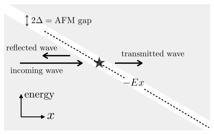
Figure 1: Energy diagram of the anti-ferromagnet subject to a DC electric field. A staggered order in lattice develops a bandgap given by the order parameter $\Delta$. A uniform electric field $E$ is incorporated as a potential ramp throughout the system. Thus, the gap acts as a potential barrier for an incident wave approaching with the velocity $v_{0}$, which splits into a reflected and transmitted wave. In the small-gap large-field limit, the amplitude of the transmitted wave is proportional to the square-root of the Landau-Zener factor ${\rm e}^{-\pi\alpha/2}$ with $\alpha=\Delta^{2}/v_{0}E$.

II.2.2 Analytic Solution

We can solve for the eigen-function $\phi^{\lambda}_{+}$ by eliminating $\phi^{\lambda}_{-}$ in the coupled equations (26) to obtain the second-order differential equation

$$v_{0}^{2}\partial_{x}^{2}\phi^{\lambda}_{+}+[(\omega+Ex)^{2}-{\rm i}v_{0}E-\Delta^{2}]\phi^{\lambda}_{+}=0.$$ (31)

Similarly to Zener’s original paper Zener (1932), we use the variables

$$z\equiv(2E/v_{0})^{1/2}{\rm e}^{{\rm i}\pi/4}(x+\omega/E)\mbox{ and }n\equiv{\rm i}\Delta^{2}/(2v_{0}E)-1$$ (32)

to transform Eq. (31) to the standard form

$$\frac{{\rm d}^{2}\phi^{\lambda}_{+}(z)}{{\rm d}z^{2}}+\left(n+\frac{1}{2}-\frac{1}{4}z^{2}\right)\phi^{\lambda}_{+}(z)=0.$$ (33)

The solutions of this equation can be expressed in terms of the parabolic cylinder function Whittaker and Watson (1920); Gradshteyn and Rhizyk (2007) as

$$\phi^{\lambda}_{+}(x+\omega/E)\propto D_{-n-1}(\pm{\rm i}z),$$ (34)

with $D_{-n-1}({\rm i}z)$ decaying to zero for $z\to{\rm e}^{-{\rm i}\pi/4}\times\infty$ and $z\to{\rm e}^{-{\rm i}(3\pi/4)}\times\infty$. We choose the sign in the argument of the parabolic cylinder function in Eq. (34) according to the boundary condition of right- or left-incident wavefunction. A more detailed discussion is given in Appendix A. The normalized solution for the right-moving wavefunction can be written down as

$$\phi^{R}_{+}(x,\omega)={\rm e}^{-3\pi\alpha/8}D_{-{\rm i}\alpha/2}\left(2y\,{\rm e}^{-{\rm i}\pi/4}\right),$$ (35)

where we introduced the dimensionless parameters

$$\alpha\equiv\frac{\Delta^{2}}{v_{0}E}\mbox{ and }y\equiv\sqrt{\frac{E}{2v_{0}}}\left(x+\frac{\omega}{E}\right).$$ (36)

Similarly, the eigen-function $\phi^{\lambda}_{-}(x,\omega)$ is given by

$$\phi^{R}_{-}(x,\omega)=-\sqrt{\frac{\alpha}{2}}{\rm e}^{-{\rm i}\pi/4}{\rm e}^{-3\pi\alpha/8}D_{-{\rm i}\alpha/2-1}\left(2y\,{\rm e}^{-{\rm i}\pi/4}\right).$$ (37)

The left-moving solutions are obtained by symmetry:

$$\phi^{L}_{-}(x,\omega) = [\phi^{R}_{+}(-x,-\omega)]^{*}={\rm e}^{-3\pi\alpha/8}D_{{\rm i}\alpha/2}\left(-2y\,{\rm e}^{{\rm i}\pi/4}\right),$$

$$\phi^{L}_{+}(x,\omega) = -[\phi^{R}_{-}(-x,-\omega)]^{*}.$$ (38)

III Landau-Zener vs. In-Gap Tunneling Regimes

We shall now distinguish two regimes: (i) the weakly gapped case, when $\alpha={\Delta^{2}}/{v_{0}E}\ll 1$, for which the nonequilibrium excitations will be shown to be dominated by Landau-Zener tunneling events; (ii) the strongly gapped case, when $\alpha\gg 1$, dominated by the excitation of dissipative in-gap states.

The distinct behaviors in these two regimes of (a) the local density of states and, (b) the energy distribution function, are illustrated in FIG. 2 which gives the numerical solutions computed at a fixed $E=0.05$ for increasing values of $\Delta$. Quite naturally, the local density of states in FIG. 2(a) continuously develops an energy gap on the order $\Delta$. In the small gap (or large field) limit, the gap is filled up by the accelerating electrons, as shown by the smearing of the gap. Perhaps less obvious is the presence of a small but finite density of in-gap states at $|\omega|\lesssim\Delta$ in the large-gap, small-field limit. We shall see that they are due to the dissipation which, in our model, broadens the two bands and make them leak inside the gap. They could also be due to the presence of impurities in the system. The distribution functions in FIG. 2(b) displays a rapid crossover between a hot nonequilibrium steady state at small $\Delta$, and a cooler state where excitations are localized in $|\omega|\lesssim\Delta$ at large $\Delta$.

Below, we elucidate the different mechanisms at stakes, and their associated energy scales, by deriving the analytic solutions of the nonequilibrium steady states in the two regimes.

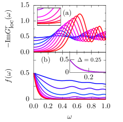
Figure 2: (a) Local density of states $-\mbox{Im }\,G^{r}_{\rm loc}(\omega)$ at $E=0.05$, $\Gamma=0.01$, with $\Delta$ varying from $0.05$ (blue) to 0.5 (red) in steps of 0.05. The energy unit is set by $v_{0}=1$. While the energy gap rapidly develops with increasing $\Delta$, the inset (blown up near zero energy) reveals the presence of a finite density of in-gap states on the order of $\Gamma/(2\Delta v_{0})$ (see text for details). (b) Distribution functions $f(\omega)$. The inset shows the agreement with the analytic result $f(\omega)\simeq\frac{1}{2}{\rm e}^{-2\Delta\omega/v_{0}E}$ (black line) computed for large $\Delta$, already at $\Delta=0.25$.

III.1 Landau-Zener Tunneling Regime

In the small $\alpha=\Delta^{2}/v_{0}E\ll 1$ regime, an asymptotic expression of the wave function in Eq. (35) can be worked out when $|y|\gtrsim\alpha$, reading

$$\phi^{R}_{+}(y<0) \simeq {\rm e}^{{\rm i}y^{2}}|2y|^{-{\rm i}\frac{\alpha}{2}}+\frac{\sqrt{2\pi}{\rm e}^{-\frac{\pi}{4}(\alpha-{\rm i})}}{\Gamma(\frac{{\rm i}\alpha}{2})}{\rm e}^{-{\rm i}y^{2}}|2y|^{{\rm i}\frac{\alpha}{2}-1}$$

$$\phi^{R}_{+}(y>0) \simeq {\rm e}^{-\frac{\pi\alpha}{2}}{\rm e}^{{\rm i}y^{2}}(2y)^{-{\rm i}\frac{\alpha}{2}},$$ (39)

where $\Gamma(x)$ is the Gamma function. For convenience, let us focus on $\omega>0$. The first term in the above expression of $\phi^{R}_{+}(y<0)$ is the incident wave from $-\infty$. Indeed, it becomes the free propagating wave computed in Eq. (17) in the limit $\alpha\to 0$. See also FIG. 1 for a brief discussion. The second term is the reflected wave which is scattered from the gap. The term in $\phi^{R}_{+}(y>0)$ represents the transmitted wave. For small $\alpha$, the amplitude of the reflected wave is small with $|\sqrt{2\pi}{\rm e}^{-\pi\alpha/4}/\Gamma({\rm i}\alpha/2)|^{2}\simeq\pi\alpha^{2}/2$ and it can be neglected for $|y|\gg 1$. We may then approximate the right-moving wavefunction for all $|y|\gtrsim\alpha$ by

$$\phi^{R}_{+}(x,\omega)\simeq{\rm e}^{{\rm i}y^{2}}(2y\,{\rm e}^{-{\rm i}\pi})^{-{\rm i}\alpha/2}.$$ (40)

$y$ is analytically continued to the complex plane with its phase restricted to $0\leq{\rm arg}(y)<\pi$, with the branchcut on the negative real axis. Then, on the positive real axis $y>0$, the factor $({\rm e}^{-{\rm i}\pi})^{-{\rm i}\alpha/2}={\rm e}^{-\pi\alpha/2}$ gives the Landau-Zener amplitude reduction while on the negative axis the factor is cancelled out.

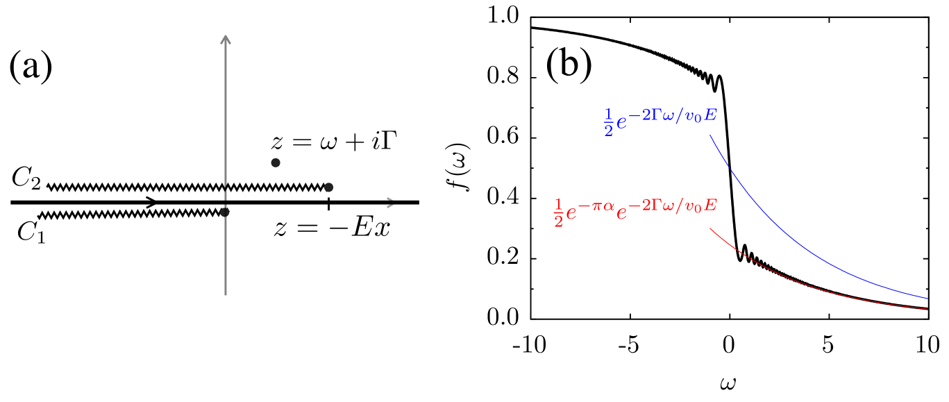
Figure 3: (a) Singularities in the integral of the retarded GF, Eq. (41), in the Landau-Zener regime using the asymptotic expansion of the parabolic cylinder function. (b) Nonequilibrium distribution function $f(\omega)$ of the driven-dissipative AF computed numerically in the Landau-Zener tunneling (LZT) regime, and compared to the expression derived in Eq. (46), showing a number of nonequilibrium excitations which is reduced by the factor ${\rm e}^{-\pi\alpha}$ compared to the single-band metal.

For $\omega>0$, and in the small-$\alpha$ limit, the right-moving wavefunctions traveling from $x<0$ contribute the most to the lesser GFs in Eq. (29). We may therefore approximate the retarded GF by

$$G^{r}_{++}(0,x;\omega)=\int_{-\infty}^{\infty}\frac{\rho_{++}(0,x;\omega^{\prime})}{\omega-\omega^{\prime}+{\rm i}\Gamma}\frac{{\rm d}\omega^{\prime}}{2\pi v_{0}},$$ (41)

with

$$\rho_{++}(0,x;\omega^{\prime})\simeq {\rm e}^{-\pi\alpha}{\rm e}^{-{\rm i}\frac{E}{2v_{0}}(x^{2}+2x\omega^{\prime}/E)}$$

$$\times\omega^{\prime-{\rm i}\alpha/2}(\omega^{\prime}+Ex)^{{\rm i}\alpha/2}.$$ (42)

As represented in FIG. 3(a), there are two branchcuts: $C_{1}\equiv(-{\rm i}\epsilon,-\infty-{\rm i}\epsilon)$ for $\omega^{\prime{\rm i}\alpha/2}$ and $C_{2}\equiv(-x+{\rm i}\epsilon,-\infty+{\rm i}\epsilon)$ for $(\omega^{\prime}+Ex)^{-{\rm i}\alpha/2}$. This choice of branchcuts ensures that the complex power functions coincide with the integrand everywhere on the real axis. The main contribution to the integral is the residue at $\omega^{\prime}=\omega+{\rm i}\Gamma$, and we detail its computation in the Appendix B. The resulting retarded GF for $x\lesssim-(2v_{0}/E)^{1/2}\alpha$ is approximately

$$G^{r}_{++}(0,x;\omega) \simeq \frac{-{\rm i}}{v_{0}}{\rm e}^{-\frac{{\rm i}Ex^{2}}{2v_{0}}-\frac{(\Gamma-{\rm i}\omega)|x|}{v_{0}}}$$ (43)

$$\times\left|\frac{\omega+{\rm i}\Gamma}{\omega-E|x|+{\rm i}\Gamma}\right|^{-{\rm i}\alpha/2}{\rm e}^{-\alpha\varphi/2},$$

where

$$\varphi=\pi-\tan^{-1}\frac{\Gamma}{\omega}-\tan^{-1}\frac{\Gamma}{E|x|-\omega}.$$ (44)

Note that Eq. (43) is invalid at $x=0$ and therefore cannot be used to compute $G^{r}_{\rm loc}(\omega)$. As shown in FIG. 2(a) for small $\alpha$, the spectral function approaches the simple-metal limit, $-{\rm Im}G^{r}_{\rm loc}(\omega>\Delta)\approx 1/(2v_{0})$, away from the gap.

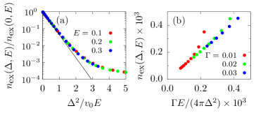
Figure 4: Number of electronic excitations $n_{\rm ex}(\Delta,E)$. (a) In the small-gap (or large-field) regime, it follows the Landau-Zener theory (black line). (b) In the large-gap (or small-field) regime, the excitations are limited inside the gap with $n_{\rm ex}(\Delta,E)=\Gamma E/(4\pi\Delta^{2})$.

In the small damping limit, we get $\varphi\simeq\pi$, and the local lesser GF can be approximated as

$$G^{<}_{\rm loc}(\omega>0)\simeq\frac{{\rm i}}{v_{0}}\,f(\omega).$$ (45)

The energy distribution function then becomes

$$f(\omega>0)\simeq\frac{1}{2}{\rm e}^{-\pi\alpha}{\rm e}^{-2\Gamma\omega/v_{0}E}.$$ (46)

The numerical effective distribution in FIG. 3(b) shows an excellent agreement with the analytic result. The step-like drop of $f(\omega)$ near $\omega=0$ by the Landau-Zener factor demonstrates a clear departure from a thermal distribution and highlights the electronic nature of the population inversion. Compared to the driven-dissipative single-band metal studied in Section II.1, see Eq. (20), the number of excited sates is reduced by the Landau-Zener factor ${\rm e}^{-\pi\alpha}$. This is reflected in the effective temperature

$$T_{\rm eff}(\alpha\ll 1)=\sqrt{\frac{3}{2}}\frac{v_{0}E}{\pi\Gamma}{\rm e}^{-\pi\alpha},$$ (47)

which is also reduced compared to the single-band metal in Eq. (22), as well as in the numerical calculations in FIG. 4(a) which displays the total number of excitations

$$n_{\rm ex}(\Delta,E)=2\int_{0}^{D}G^{<}_{\rm loc}(\omega)\frac{{\rm d}\omega}{2\pi{\rm i}}.$$ (48)

The excitation density $n_{\rm ex}(\Delta,E)$ is defined as the electron and hole excitations from the zero-field electron distribution. Here, we introduced an energy cutoff $D$ (set to $10\,v_{0}$ throughout the paper) to regularize the linear dispersion relation. For small $\alpha$, the agreement with the Landau-Zener factor (black line) is excellent, as also previously demonstrated in the lattice model calculation Li et al. (2017).

Note that in the regime $\alpha\to 0$, the distribution function in Eq. (46) naturally boils down to the one of the single-band metal in Section II.1, see Eq. (21).

III.2 In-Gap Tunneling Regime

In the opposite regime of large $\alpha=\Delta^{2}/v_{0}E\gg 1$, i.e. with a large gap or a small field, the electronic transport proceeds quite differently. This is illustrated in FIG. 4(a) which shows a strong deviation of the total number of excitations from the Landau-Zener theory. The spectral weight inside the gap is now controlled by the dissipation, bounded from below by the zero-field spectral weight $-\mbox{Im }G^{r}_{\rm loc}(0)=\Gamma/(2v_{0}\Delta)$. The spectral properties deep inside the gap can be approximated by the zero-field retarded GF, as detailed in Appendix C. The electronic excitations are most efficient within the gap, as demonstrated by the energy distribution function $f(\omega)$ displayed in FIG. 2(b). The shape of the distribution function in this regime can be understood as follows. In the case of the single-band metal studied in Section II.1, the damping rate $\Gamma$ was controlling the energy window of the nonequilibrium excitations. In the presence of a gap, the gap acts as a potential barrier and provides a decay rate similar to the WKB theory. Therefore, the gap parameter $\Delta$ replaces $\Gamma$ in Eq. (21), leading to the energy distribution function

$$f(\omega>0)\simeq\frac{1}{2}{\rm e}^{-2\Delta\omega/v_{0}E}$$ (49)

for large $\alpha$. It is interesting to note that while dissipation is essential to create the in-gap states, the distribution function has negligible dependence on the damping parameter $\Gamma$. Noteworthy enough, while FIG. 4(a) indicates that the deviation from the Landau-Zener theory starts around $\alpha\sim 1-2$, the inset of FIG. 2(b) shows that the distribution function in Eq. (49) computed for $\alpha\gg 1$ is already valid at $\Delta=0.25$.

The corresponding effective temperature can be computed as

$$T_{\rm eff}(\alpha\gg 1)=\sqrt{\frac{3}{2}}\frac{v_{0}E}{\pi|\Delta|},$$ (50)

that is much smaller than in the LZ regime: $T_{\rm eff}(\alpha\gg 1)\ll T_{\rm eff}(\alpha\ll 1)$. The total number of nonequilibrium charge excitations is then well approximated by

$$n_{\rm ex}(\Delta,E)\simeq 2\int_{0}^{\infty}\mathrm{d}{\omega}\;\frac{\Gamma}{2\pi v_{0}\Delta}f(\omega)=\frac{\Gamma E}{4\pi\Delta^{2}},$$ (51)

which is confirmed by the numerical calculations presented in FIG. 4(b).

Note that the effective temperature above is seemingly independent of $\Gamma$. Indeed, it was computed in the regime $|\omega|\leq\Delta$ where the energy distribution is given by the expression in Eq. (49). At large frequencies $\omega\gg\Delta$, however, $f(\omega)$ is expected to behave as $\frac{1}{2}{\rm e}^{-\pi\alpha}{\rm e}^{-2\Gamma\omega/v_{0}E}$. This tail contributes a correction term proportional to ${\rm e}^{-\pi\alpha}(\Delta/\Gamma)^{2}$, which grows large in the $\Gamma\to 0$ limit. This is consistent with the previous works Eckstein et al. (2010); Eckstein and Werner (2011) in which the effective temperature has been shown to diverge in dissipationless driven systems. In the following Section, however, we limit the energy integrals at the cutoff energy $D$ and, furthermore, the decaying integrand in the gap equation renders insignificant the effect of the $f(\omega)$ tail, particularly in the large $\alpha$ limit as shown in the inset of FIG. 2(b).

IV Mean-Field Theory of Resistive Switching in Anti-Ferromagnets

In the previous Section, we discussed how, upon increasing the electric field and keeping the gap parameter $\Delta$ fixed, the electrons are initially excited via in-gap tunneling events, and then undergo Landau-Zener tunneling processes as the field is further increased. In a recent paper by the Authors Li et al. (2017), it has been shown that an inhomogeneous mean-field (MF) approach on a two-dimensional Hubbard model could capture the hysteretic nature of the true resistive switching transition: sweeping up and down the voltage bias applied on a finite-size two-dimensional lattice resulted in an insulator-to-metal transition (IMT) and a metal-to-insulator transition (MIT), separated by a region of bi-stability. Importantly, this nonequilibrium bi-stability was found to be crucial to explain the abrupt nature of the resistive switching, independently whether the parent equilibrium transition is continuous or discontinuous.

Here, we explore the mechanisms behind the IMT and the MIT via a continuum theory which allows an analytic understanding of the problem. Below, we develop the mean-field theory for a driven-dissipative anti-ferromagnet (AF). This approach may be extended to other types of order without much difficulty. We start with the standard single-orbital Hubbard model, with on-site repulsive Coulombic interaction $\hat{V}=U\sum_{i}(\hat{n}_{i\uparrow}-\bar{n})(\hat{n}_{i\downarrow}-\bar{n})$ with the electron number operator $\hat{n}_{i\sigma}=d^{\dagger}_{i\sigma}d_{i\sigma}$, the Coulomb parameter $U$, and the on-site occupation expectation value (averaged over spin) $\bar{n}$. The emergence of an AF phase corresponds to the breaking of the translational invariance of the lattice into a staggered order. The energy levels of the two resulting sublattices $A$ and $B$ get shifted alternately by $\pm\Delta$, the AF order parameter which opens a charge gap. The corresponding mean-field decoupling of the Hubbard interaction consists in replacing

$$\hat{V}\mapsto\hat{V}_{\rm MF}=\Delta\sum_{m=A/B,i_{m},\sigma}(-1)^{m}\sigma\hat{n}_{i_{m},\sigma},$$ (52)

with the sublattice index $m$ and $(-1)^{m}=\pm 1$ for $m=A$ and $B$, respectively. $\hat{n}_{i_{m}}$ is the electron occupation on the $i_{m}$-th site within the $m$-sublattice. The resulting theory is invariant under $\Delta\mapsto-\Delta$, and we may work with $\Delta\geq 0$. Since the MF Hamiltonian is diagonal in the spins, we may also afford to ignore the spin degrees of freedom in what follows. The nonequilibrium self-consistent equation on the AF order parameter, often referred as the gap equation, reads

$$\Delta =\frac{U}{2}(\langle n_{A}\rangle-\langle n_{B}\rangle)$$ (53)

$$=U\int_{-D}^{D}\left[G^{<}_{-+}(\omega)+G^{<}_{+-}(\omega)\right]\frac{{\rm d}\omega}{2\pi{\rm i}}.$$ (54)

IV.1 Equilibrium Phase Transition

For reference, let us briefly review the conditions for the equilibrium, temperature-driven, phase transition. The mean-field approach predicts a second order phase transition Slater (1951). As described in Appendix C, for $|\omega|>\Delta_{0}$ and at zero temperature, the gap equation (54) becomes

$$\frac{2\pi v_{0}}{U}=\int_{-D}^{-\Delta_{0}}\frac{{\rm d}\omega}{\sqrt{\omega^{2}-\Delta_{0}^{2}}}\simeq\ln\left(\frac{2D}{\Delta_{0}}\right),$$ (55)

in the small gap limit, $\Delta_{0}\ll D$. This yields the familiar expression for the order parameter at zero temperature and zero-field

$$\Delta_{0}\simeq 2D\exp\left(-\frac{2\pi v_{0}}{U}\right).$$ (56)

The transition temperature $T_{\rm N}$ is set by the finite-temperature gap equation

$$\frac{2\pi v_{0}}{U}=-\int_{-D}^{D}\frac{\omega f_{0}(\omega)}{\omega^{2}+\Gamma^{2}}{\rm d}\omega\simeq\ln\left(\frac{2D}{\pi T_{\rm N}}\right)+\gamma,$$ (57)

where $f_{0}(\omega)$ is the Fermi-Dirac distribution at the temperature $T_{N}$ and $\gamma\approx 0.577$ is the Euler constant. This allows to relate the Néel temperature to the zero-temperature gap via

$$T_{\rm N}\approx\frac{{\rm e}^{\gamma}}{\pi}\Delta_{0}\approx 0.57\,\Delta_{0}.$$ (58)

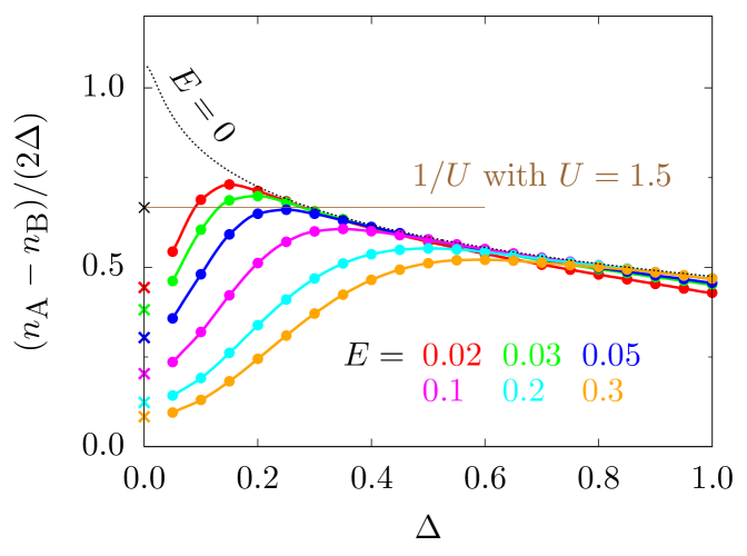
Figure 5: Nonequilibrium mean-field self-consistent condition on the order parameter $\Delta$. The solutions correspond to the intersection of the curves at different $E$-field with the $1/U$ line. The finite-$\Delta$ solutions with a negative slope are the stable solutions. The solution at $\Delta\approx 0.25$ brutally disappears at $E_{\rm MIT}=0.044$. The crosses at $\Delta=0$ are calculated as discussed in Appendix E.

IV.2 Nonequilibrium Phase Transitions

IV.2.1 Numerical Results

The numerical solutions of the nonequilibrium mean-field self-consistent gap equation are presented in FIG. 5, where the (rhs)$/(U\Delta)$ of Eq. (54) is plotted as a function of the (lhs). $\Delta=0$ is always a trivial solution, marked by crosses in the figure. It corresponds to an ungapped, metallic, phase. The intersections of the curves with $1/U$ at finite values of $\Delta$ are non-trivial solutions that correspond to anti-ferromagnetic states. In equilibrium ($E=0$), the curve (dotted line) is monotonic in $\Delta$ and thus supports a single AF solution. As $U$ is varied, the single-valued order parameter $\Delta$ evolves continuously from a vanishing to a finite value. This is the second order equilibrium phase transition. However, as $E$ is turned on, the curve becomes non-monotonic and allows two AF solutions at small enough $E$. A stability analysis indicates that the solution with the smaller $\Delta$ is unstable while the other one is stable. When $E$ becomes larger than a critical value ($E_{\rm MIT}=0.25$ in the figure with $U=1.5$), the two AF solutions suddenly disappear, leaving $\Delta=0$ as the only solution. This is the IMT: a strongly discontinuous nonequilibrium phase transition which emerges out of a continuous transition in equilibrium Li et al. (2017).

Below, we discuss the quantitative criteria for the switching electric fields at the IMT and MIT.

IV.2.2 Insulator-to-Metal Transition

As discussed above, the IMT occurs when the stable finite-$\Delta$ solution abruptly ceases to exist, at the field $E_{\rm IMT}$. We first determine in which of the regimes, Landau-Zener or in-gap tunneling, the IMT occurs. In FIG. 5, the IMT occurs at $\alpha_{\rm IMT}\approx 1.25$, thus in the crossover region between the two limiting regimes. However, as shown in the inset of FIG. 2(b), the distribution function in Eq. (49), although computed far in the in-gap tunneling regime (i.e. for $\alpha\gg 1$), describes the numerical solution fairly well. We use it, together with the approximation that the off-diagonal components of the GFs can be replaced by their equilibrium components (see Appendix D), to re-write the gap equation as

$$\frac{2\pi v_{0}}{U} =\int_{-D}^{-\Delta}\frac{{\rm d}\omega}{\sqrt{\omega^{2}-\Delta^{2}}}-\int_{\Delta}^{\infty}\frac{{\rm e}^{-2\Delta\omega/v_{0}E}}{\sqrt{\omega^{2}-\Delta^{2}}}{\rm d}\omega,$$ (59)

or, equivalently,

$$0 =\ln\left(\frac{\Delta}{\Delta_{0}}\right)+K_{0}\left(\frac{2\Delta^{2}}{v_{0}E}\right).$$ (60)

See the derivation of Eq. (106) in Appendix for more details. $K_{n}(x)$ is the modified Bessel function of the second kind. The first term of the (rhs) in Eqs. (59) and (60) is the equilibrium contribution, and the second term is the reduction of the order parameter due to the nonequilibrium excitations where the main contribution originates from the edge of the gap $\omega\simeq\Delta$.

Threshold field.

The condition for the IMT is that the derivative of the rhs of the above equation with respect to $\Delta$ vanishes at the solution, i.e. $1+4\alpha K_{0}^{\prime}(2\alpha)=0$. This yields $\alpha_{\rm IMT}\approx 0.63$. Note the relative discrepancy with the numerical result given above, $\alpha_{\rm IMT}\approx 1.25$. It shows that the analytic derivation underestimates $\Delta_{\rm IMT}$ and overestimates $E_{\rm IMT}$, due the piece of integral that was neglected inside the gap. Substituting the analytic result $\alpha_{\rm IMT}\approx 0.63$ into Eq. (60), we obtain

$$\Delta_{\rm IMT}\simeq{\rm e}^{-K_{0}(2\alpha_{\rm IMT})}\Delta_{0}\approx 0.74\,\Delta_{0},$$ (61)

and

$$E_{\rm IMT}=\frac{\Delta_{\rm IMT}^{2}}{\alpha_{\rm IMT}v_{0}}\approx 0.88\,\frac{\Delta_{0}^{2}}{v_{0}}.$$ (62)

From the numerical calculations with $U=1.5$, we have $\Delta_{0}=0.30$, $E_{\rm IMT}=0.044$ and $\Delta_{\rm IMT}=0.23$, yielding the ratios $\Delta_{\rm IMT}\approx 0.76\,\Delta_{0}$ and $E_{\rm IMT}\approx 0.49\,(\Delta_{0}^{2}/v_{0})$, which are in a reasonable agreement with the analytic estimates.

Importantly, these results elucidate a long standing problem: the puzzling small values of the electric field that are needed to achieve the IMT. Indeed, our solution shows that

$$E_{\rm IMT}/\Delta_{0}\sim\Delta_{0}/v_{0}\ll 1,$$ (63)

i.e. that the energy scale of the switching field can be up to one order of magnitude smaller than the energy gap. However, with a typical $\Delta_{0}\sim 0.1$ eV and $\hbar v_{0}/a\sim 1$ eV, this corresponds to switching fields on the order of $E_{\rm IMT}\sim 10^{2}$ kV/cm which are still one to two orders of magnitude larger than what is observed experimentally. We have seen in the previous work Li et al. (2017) that nucleation of conducting filament in spatially inhomogeneous systems reduces $E_{\rm IMT}$ significantly. We shall also argue in Sect. IV.3 that the remaining discrepancy can be much reduced by working with an environment at a finite temperature $T_{\rm b}\lesssim T_{\rm N}$ rather than $T_{\rm b}=0$, i.e. by bringing the equilibrium system closer to its Néel transition, which is the case in most experiments.

Effective temperature at the transition.

Another crucial test for the theory is the ability to predict that the effective electronic temperature at the IMT matches the equilibrium transition temperature $T_{\rm N}$, as it has recently been demonstrated experimentally Zimmers et al. (2013). From Eqs. (16) and (49), we obtain the analytic estimate

$$T_{\rm IMT}=\frac{\sqrt{6}}{2\pi}\frac{v_{0}E_{\rm IMT}}{\Delta_{\rm IMT}}\approx 0.46\,\Delta_{0}\approx 0.81\times T_{\rm N}.$$ (64)

The numerical results give $T_{\rm IMT}=0.163=0.54\,\Delta_{0}\approx 0.95\times T_{\rm N}$, in very good agreement with the previous numerical work Li et al. (2017) on discrete lattices. This proves that the effective temperature at which the IMT occurs is simply controlled by $T_{\rm N}$, the equilibrium transition temperature. This is one of the main result of this work, which justifies recent experimental observations made in Ref. Zimmers et al. (2013).

The IMT condition can be roughly understood as the situation when the tail of the electron distribution in Eq. (49) begins to overlap with density of states at the edge of the gap, $v_{0}E/(2\Delta)\sim\Delta$ i.e. $\alpha\sim 0.5$, and the number of nonequilibrium excitations is about to proliferate. It is remarkable that, despite the IMT occurring in the crossover region between the Landau-Zener and the in-gap tunneling regimes, the IMT conditions do not depend sensitively on the dissipation parameter $\Gamma$. This clearly indicates that the IMT is fundamentally an electronic process, while it also permits a thermal interpretation.

$I-V$ scaling near the IMT.

Based on the gap equation in Eq. (60), we can analyze the limiting behavior near the IMT. Writing $\Delta=\Delta_{\rm IMT}+\delta\Delta$ and $E=E_{\rm IMT}+\delta E$, and expanding the gap equation to the lowest orders, we obtain

$$0=1.86\,\frac{(\delta\Delta)^{2}}{2\Delta_{\rm IMT}^{2}}+\frac{\delta E}{2E_{\rm IMT}},$$ (65)

which can be massaged to the typical MF scaling relation

$$\delta\Delta\simeq\alpha_{\rm IMT}(-v_{0}\,\delta E)^{1/2}\mbox{ for }\delta\Delta>0,\,\delta E<0.$$ (66)

Furthermore, the GFs do not have any singularities when $\Delta$ and $E$ pass through $\Delta_{\rm IMT}$ and $E_{\rm IMT}$, as can be seen in FIG. 2. Therefore, we may expand the electric current $J$ around its value right before the IMT in powers of $\delta\Delta$ and $\delta E$,

$$J(E,\Delta) \simeq J_{\rm IMT}+a_{E}\,\delta E+a_{\Delta}\,\delta\Delta$$ (67)

$$\simeq J_{\rm IMT}-\alpha_{\rm IMT}|a_{\Delta}|(-v_{0}\,\delta E)^{1/2},$$

where $a_{E}$ and $a_{\Delta}$ are expansion coefficients. Since the current is reduced when the gap increases, we must have $a_{\Delta}<0$. While the precise value of the above critical exponent in the current characteristic is the result of a mean-field approach, and might therefore get final-dimensional corrections, such a non-analytic and rapid increase of the current close to the IMT is a universal prediction of the theory. As a matter of fact, it has already been observed in our previous numerical lattice simulation Li et al. (2017) and in recent experiments Zimmers et al. (2013); Doron et al. (2016), and deserves closer scrutiny.

IV.2.3 Metal-to-Insulator Transition

Threshold field.

The MIT is determined by the loss of stability of the $\Delta=0$ solution. In FIG. 5, the threshold $E_{\rm MIT}$ corresponds to when the curve at $\Delta=0$ (black cross) matches $1/U$. The stability of the metal is given by the condition

$$\frac{1}{U}\geq\lim_{\Delta\to 0}\frac{1}{2\Delta}(n_{A}-n_{B}).$$ (68)

We can easily and accurately pinpoint the MIT by using perturbation theory in the small $\Delta$ limit. The details are given in Appendix E. Equation (68) can be estimated as

$$\frac{1}{U}\gtrsim\frac{1}{2\pi v_{0}}\ln\left(\frac{2\gamma\Gamma D}{v_{0}E}\right),$$ (69)

which typically overestimates the exact numerical integrals by less than 5%. It yields a switching field

$$E_{\rm MIT}=1.78\,\frac{\Gamma}{v_{0}}\Delta_{0}.$$ (70)

From the numerical calculations with $U=1.5$ and $\Gamma=0.01$, we obtained $E_{\rm MIT}=0.0044$ yielding the ratio $E_{\rm MIT}=1.46\,(\Gamma/v_{0})\Delta_{0}$ which is, again, in good agreement with the analytic estimate. Equation (70) reveals that, unlike the IMT, the MIT crucially depends on the dissipation, which is not surprising since the transition is initiated from a metallic phase where Joule heating is non-negligible. Most importantly, this also shows that $E_{\rm MIT}\sim(\Gamma/\Delta_{0})E_{\rm IMT}$, therefore predicting the hierarchy

$$E_{\rm MIT}\ll E_{\rm IMT}\ll\Delta_{0}.$$ (71)

Effective temperature at the transition.

Coming from a metallic regime, the effective temperature corresponds to the one computed in Eq. (22). We obtain the following analytic estimate

$$T_{\rm MIT}\approx 1.22\times T_{\rm N},$$ (72)

where $T_{\rm N}$ is the equilibrium Néel temperature. Once again, this validates the idea that the resistive transitions can be interpreted in the language of thermal transitions where the temperature is replaced by an effective temperature accounting for the number of excitations above the chemical potential. Noteworthy, while our homogeneous mean-field approach cannot capture it, the bi-stability region has already been shown to support the formation of metallic filaments (and insulating domains) at lower effective temperatures Li et al. (2017), i.e. at lower threshold fields than the above mean-field prediction (72).

IV.3 RS at Finite Bath Temperature

So far, we have limited our theoretical analysis to the case of a zero-temperature bath, $T_{\rm b}=0$, and found switching fields one to two orders of magnitude larger than what is typically observed in experiments (see the discussion in Sect. IV.2). However, the experimental measurements of the RS are often conducted close to room temperature. Indeed, at low temperature the switching fields tend to be fairly large, which is difficult to realize and can damage the samples. Moreover, two experimental observations are worth mentioning. First, as reported previously Wu et al. (2011); Singh et al. (2015), the switching fields $E_{\rm IMT}$ and $E_{\rm MIT}$ show a significant temperature dependence, for instance with $E_{\rm IMT}$ varying by a factor of two over 30 K near the Néel temperature in VO₂ Singh et al. (2015). Second, it has recently been reported in the superconductor-insulator switching Doron et al. (2016) that the nonequilibrium phase transition displays critical behaviors similar to the equilibrium liquid-gas transition close to its critical temperature, with a strong temperature dependence of the switching electric field. All these considerations lead us to investigate the case of a finite-temperature bath, $T_{\rm b}>0$. We shall show that increasing $T_{\rm b}$ naturally corresponds to a higher effective temperature $T_{\rm eff}(T_{\rm b})$, bringing the system closer to its transition, therefore reducing the threshold fields and the intensity of the nonequilibrium effects. As the bath temperature reaches the Néel temperature, $T_{\rm b}\to T_{\rm N}$, the threshold fields must vanish, $E_{\rm IMT/IMT}\to 0$, and the nonequilibrium RS is expected to progressively evolve into the continuous Ising transition of the equilibrium Néel transition.

IV.3.1 Single-Band Metal

We first discuss the impact of a finite temperature of the environment in the case of the single-band metal studied in Section II.1. The equation (14) is generalized to

$$G^{<}_{\rm loc}(\omega)=2{\rm i}\Gamma\int_{-\infty}^{\infty}\mathrm{d}{x}\;\frac{1}{2}\sum_{\lambda}|G^{r}_{\lambda}(0,x;\omega)|^{2}f_{0}(\omega+Ex),$$ (73)

where $f_{0}(\omega)$ is the Fermi-Dirac distribution function at temperature $T_{\rm b}$. Using the definition of the effective temperature in Eq. (16) and the following identity Kirillov (1994)

$$\int_{0}^{\infty}\omega[f_{0}(\omega+Ex)+f_{0}(\omega-Ex)]{\rm d}\omega=\frac{1}{2}(Ex)^{2}+\frac{1}{6}(\pi T_{\rm b})^{2}$$ (74)

for an arbitrary bath temperature $T_{\rm b}$, we obtain the following effective temperature for the electric-field driven one-dimensional electron gas coupled to a finite-temperature bath

$$T_{\rm eff}(T_{\rm b})^{2}=\frac{3}{2}\left(\frac{v_{0}E}{\pi\Gamma}\right)^{2}+T_{\rm b}^{2}=T_{\rm eff}(0)^{2}+T_{\rm b}^{2}.$$ (75)

Note that this relation can also be obtained by using the energy balance between the Joule heating and the heat dissipation that compensate each other in the steady state Altshuler et al. (2009).

IV.3.2 Finite-Temperature IMT

We now turn to the case of the driven-dissipative anti-ferromagnet. To compute the temperature dependence of the threshold field, $E_{\rm IMT}(T_{\rm b})$, we use perturbation theory in $T_{\rm b}$ around the previous results obtained at $T_{\rm b}=0$. Using the small-field approximations developed in Appendix C, we can generalize the gap equation in Eq. (60) to

$$0=\ln\left(\frac{\Delta}{\Delta_{0}}\right)+\left[1+\frac{2}{3}\left(\frac{\pi T_{\rm b}\Delta}{v_{0}E}\right)^{2}\right]K_{0}\left(\frac{2\Delta^{2}}{v_{0}E}\right).$$ (76)

where we assumed $T_{\rm b}\ll T_{\rm eff}(0)\sim v_{0}E/\Delta$. Using the same criteria as Section IV.2, the IMT can be parametrically solved as

$$\frac{v_{0}E_{\rm IMT}}{\Delta_{0}^{2}} = \frac{2}{u}{\rm e}^{-h(u)},$$

$$\frac{\pi T_{\rm b}}{\Delta_{0}} = \left(\frac{3(1-2uK_{1})}{u^{2}(uK_{1}-K_{0})}\right)^{1/2}{\rm e}^{-h(u)/2},$$ (77)

with $K_{0}=K_{0}(u)$, $K_{1}=K_{1}(u)$ and $h(u)=(1-2K_{0})K_{0}/(uK_{1}-K_{0})$. The solution is plotted with a black dashed line in FIG. 6. By expanding the relations around $T_{\rm b}=0$, we obtain the following expression for the $E_{\rm IMT}$,

$$E_{\rm IMT}(T_{\rm b})\simeq E_{\rm IMT}(0)\left[1-0.88\left(\frac{T_{\rm b}}{T_{\rm N}}\right)^{2}\right]\mbox{ for }T_{\rm b}\ll T_{\rm N}.$$ (78)

A numerical evaluation of $E_{\rm IMT}(T_{\rm b})$, represented by black circles in FIG. 6, confirms its relatively slow decrease as the bath temperature is increased. At higher temperatures, $T_{\rm b}\sim T_{\rm N}$, the parametric solution in Eq. (78) ceases to be valid, and the numerical calculations are very hard to converge, preventing us to resolve how $E_{\rm IMT}(T_{\rm b})$ approaches 0 when $T_{\rm b}\to T_{\rm N}$. However, measurements in Ref. Wu et al. (2011) reported that the relation $E_{\rm IMT}(T_{\rm b})$ displays an exponential dependence with the bath temperature close to $T_{\rm N}$, and therefore a rapid decrease of $E_{\rm IMT}(T_{\rm b})$ near $T_{\rm b}\approx T_{\rm N}$ is expected.

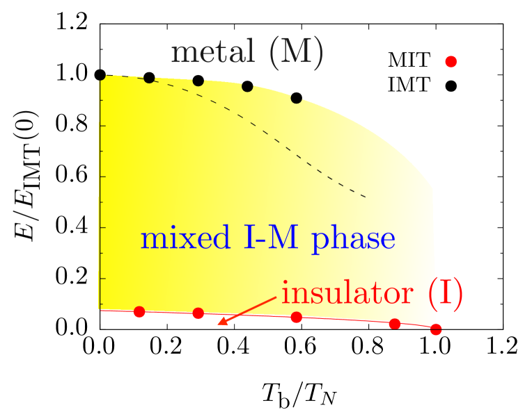
Figure 6: Phase diagram in (electric field)-(bath temperature) space. Numerically computed switching fields are shown as circles at the bath temperature $T_{\rm b}$ for the IMT (black) and MIT (red). The dashed line is the analytic result Eq. (77), and the red solid line Eq. (79). $T_{\rm N}$ is the Néel temperature at equilibrium, and $E_{\rm IMT}(0)\approx 0.044$ the numerically estimated value at zero bath temperature.

IV.3.3 Finite-Temperature MIT

The temperature dependence of the MIT is easier to analyze. Since the MIT concerns the stability of the metallic phase, the effective temperature relation derived in Eq. (75) holds at the MIT. This yields

$$E_{\rm MIT}(T_{\rm b})=\sqrt{\frac{2}{3}}\frac{\pi\Gamma}{v_{0}}\sqrt{T_{\rm N}^{2}-T_{\rm b}^{2}},$$ (79)

and at high temperatures close to $T_{\rm N}$, it yields the scaling relation

$$E_{\rm MIT}(T_{\rm b})\simeq E_{\rm MIT}(0)\sqrt{\frac{T_{\rm N}-T_{\rm b}}{T_{\rm N}}}.$$ (80)

Our theory thus successfully reproduces the square-root behavior $E_{\rm MIT}(T_{\rm b})$ near $T_{\rm N}$ which had been observed experimentally Wu et al. (2011). Numerically, the same procedure as described in Appendix E can be used, computing the off-diagonal GF in Eq. (54) as

$$-\int_{-\infty}^{\infty}\frac{2\Gamma\Delta\omega}{v_{0}^{4}(k_{1}^{2}+k_{2}^{2})}{\rm e}^{-2k_{2}|x|}f_{0}(\omega+Ex){\rm d}x,$$ (81)

with $k_{1,2}$ given in Eq. (101) and the Fermi-Dirac function $f_{0}(\omega)$ at temperature $T_{\rm b}$. The oscillatory parts of the off-diagonal GF are ignored in this calculation. The numerical results for $E_{\rm MIT}(T_{\rm b})$ are shown with red circles, validating furthermore the above square-root scaling relation.

The mean-field theory seems to predict a very slow decrease of $E_{\rm IMT}(T_{\rm b}\ll T_{\rm N})$, as depicted in FIG. 6. Consequently, it predicts a wide bi-stability region where both metallic and insulating phases can coexist. One has to keep in mind that a mean-field approach typically exaggerates the domain of stability of ordered states, and only a more sophisticated diagrammatic theory could resolve this issue. We emphasize that the bath-temperature dependence at the RS is significant even when the underlying mechanism is electronic, and a large reduction of the switching field over an order of $\Gamma/\Delta_{0}$ should be carefully taken into interpretation when the energy scale of switching field is examined.

V Towards an Effective Field Theory of Resistive Switching

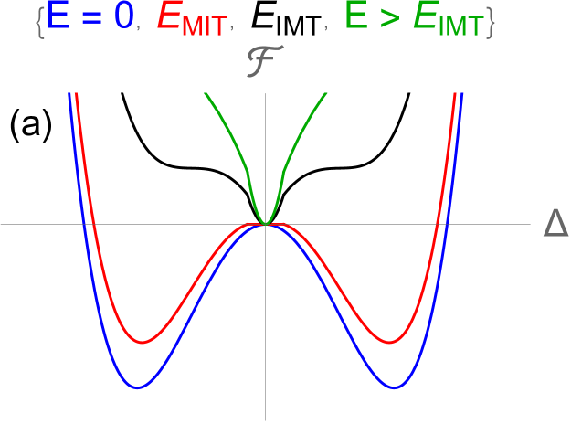
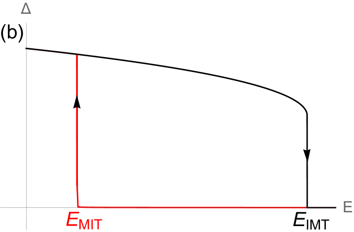
Figure 7: (a) Shape of the effective free energy $\mathcal{F}(\Delta)$ proposed in Eq. (85) when varying the electric field $E$. (b) Corresponding spontaneous order parameter $\Delta$, when varying $E$. The hysteresis, and the bi-stability region between the MIT and the IMT, emerge naturally from the two regimes of effective temperature given in Eq. (88).

In this Section, we leverage the teachings of the previous mean-field analysis to propose a low-energy effective theory description of the local order parameter $\Delta$ at both the MIT and the IMT. This could provide a practical path to developing an effective field theory capturing the spatial fluctuations of the order parameter, which are critical to the understanding of realistic resistive switching phenomena. The problem being far from equilibrium, such an effective theory should not only determine the gap $\Delta$ (a spectral quantity obtained from $G^{r}$), but also the nonequilibrium excitations (such as the quantity $T_{\rm eff}$, obtained from the ratio of $G^{<}$ and $G^{r}$). In principle, only a fully nonequilibrium approach such as the quantum Schwinger-Keldsyh formalism or the classical Martin-Siggia-Rose formalism Martin et al. (1973); Schmittmann and Zia (1995) can tackle both order parameters, $\Delta$ and $T_{\rm eff}$, on an equal footing. However, we aim at a simpler description by constructing an effective Ginzburg-Landau free energy for $\Delta$ alone, $\mathcal{F}(\Delta)$, under a finite electric field. Instead of being a dynamical quantity, the effective temperature will be fixed by using an educated ansatz, $T_{\rm eff}(\Delta)$, based on the results of the previous Sections. Although certainly less rigorous than a Schwinger-Keldsyh or Martin-Siggia-Rose approach, this static approach does not require solving time dynamics, giving a huge computational advantage when extending the theory to large heterogeneous systems including phase segregation Li et al. (2017).

The functional form of ${\cal F}(\Delta)$ is dictated by the $\mathbb{Z}_{2}$ symmetry of the order parameter, and its minima and their stability are imposed by the gap equation,

$$\mbox{zeros}\left\{\frac{{\rm d}{\cal F}(\Delta)}{{\rm d}\Delta}\right\}=$$

$$\ \mbox{zeros}\left\{\Delta-U\int_{-D}^{D}\!\frac{{\rm d}\omega}{2\pi{\rm i}}\left[G^{<}_{-+}(\omega)+G^{<}_{+-}(\omega)\right]\right\},$$ (82)

$$\mbox{sign}\left\{\frac{{\rm d}^{2}{\cal F}(\Delta)}{{\rm d}\Delta^{2}}\Big{|}_{\mbox{zeros}}\right\}=$$ (83)

$$\ \mbox{sign}\left\{1-U\int_{-D}^{D}\!\frac{{\rm d}\omega}{2\pi{\rm i}}\frac{{\rm d}}{{\rm d}\Delta}\left[G^{<}_{-+}(\omega)+G^{<}_{+-}(\omega)\right]\Big{|}_{\mbox{zeros}}\right\}.$$

Another constraint on ${\cal F}(\Delta)$ comes from the equilibrium limit ($E=0$) for which the Ginzburg-Landau free energy is an Ising $\phi^{4}$-theory reading

$$\mathcal{F}_{\rm eq}(\Delta)=(T-T_{\rm N})\,\Delta^{2}+\lambda\,\Delta^{4}+\ldots$$ (84)

where $T$ is the temperature of the system, and $T_{\rm N}$ is the Néel temperature at which the equilibrium transition occurs. The interaction parameter $\lambda>0$ can be set by requiring that $\Delta=\Delta_{0}$ at zero temperature, yielding $\lambda\approx T_{\rm N}/2\Delta_{0}^{2}$. All these constraints lead us to propose the following effective Ginzburg-Landau free energy

$$\mathcal{F}(\Delta)=\left(T_{\rm eff}(\Delta)-T_{\rm N}\right)\Delta^{2}+\lambda\,\Delta^{4}+\ldots$$ (85)

with the state-dependent effective temperature given, at zero bath temperature, by the expressions in Eqs. (22) and (50),

$$T_{\rm eff}(\Delta)\sim\left\{\begin{array}[]{l}v_{0}E/\Gamma\mbox{ {\rm i}n the small }\Delta\mbox{ regime,}\\ v_{0}E/|\Delta|\mbox{ {\rm i}n the large }\Delta\mbox{ regime.}\end{array}\right.$$ (88)

Importantly, the electric field now enters the problem solely through the renormalization of the temperature to a gap-dependent effective temperature $T_{\rm eff}(\Delta)$. This constitutive relation is the only remainder of the nonequilibrium nature of the problem. The distance to the Néel temperature $T_{\rm N}$ in the $\Delta^{2}$ term controls the stability of the metallic phase at $\Delta=0$. In the spirit of an effective field-theory description, the coefficients of the higher order terms are expected to play an irrelevant role near the transitions, merely renormalizing the transition temperatures.

Interestingly enough, in the large $\Delta$ regime, the electric field couples to the order parameter linearly via the non-analytic term $E|\Delta|$, which transforms the continuous equilibrium phase transition into a discontinuous resistive switching. In this Ginzburg-Landau language, the MIT and IMT correspond to the destabilization of a metastable solution, i.e. to the disappearing of a local minimum of $\mathcal{F}(\Delta)$ to the profit of a global minimum. For example, at the IMT the insulating solution at $\Delta\approx\Delta_{0}/\sqrt{3}$ is destabilized when the effective temperature reaches

$$T_{\rm IMT}\approx\frac{4}{3}T_{\rm N},$$ (89)

which is naturally consistent with our previous findings, see Eq. (64), up to small differences in the numerical factors due to the truncation of the free energy to lowest orders. The conclusion that $T_{\rm IMT}$ is controlled by $T_{\rm N}$ is valid regardless of the precise $E$-field dependence in Eq. (88) as long as $T_{\rm eff}(\Delta)\propto 1/\Delta$ at large $\Delta$.

FIG. 7 sketches the evolution of the shape of $\mathcal{F}(\Delta)$, when increasing $E$ starting from a stable insulating state ($\Delta>0$), rapidly developing a second stable minimum at $\Delta=0$ which becomes the only stable minimum at $E_{\rm IMT}$, when the insulating state becomes unstable. When decreasing the electric field from this metallic state, the stability of the latter is lost at a much lower electric field $E_{\rm MIT}\sim(\Gamma/\Delta_{0})E_{\rm IMT}$.

VI Conclusions

We have worked out an analytic window into the inner workings of RS in correlated insulators close to an equilibrium phase transition by means of a mean-field (MF) treatment of a minimal model of a driven-dissipative anti-ferromagnet. This allowed to unambiguously resolve the age-old debate on whether the RS is mainly electronically driven or thermally driven: both scenarios were reconciled in a unified picture where the nonequilibrium electronic excitations were characterized by a state-dependent effective temperature $T_{\rm eff}$. While the underlying physical mechanism responsible for the latter is different in the insulating state (mostly electronic Landau-Zener events) from that of the metallic state (mostly thermal heating caused by the dissipative mechanisms), both the IMT and the IMT were shown to occur whenever $T_{\rm eff}$ reaches $T_{\rm N}$, the equilibrium Néel transition temperature. Concomitantly, our analytics also provided an elegant resolution to the puzzle posed by the disconcertingly small threshold fields when compared to the typical spectral energy scales: the electric field does not affect substantially the spectrum of the materials, but enters the problem through the effective temperature $T_{\rm eff}$. While the latter is comparable to the bandgap at the RS, the electric field can be orders of magnitude smaller.

While the analytic MF approach makes the theory transparent, the range of validity of the MF approximation in nonequilibrium situations is largely untested. Although the agreement with many salient experimental features is very encouraging Li et al. (2017), our theoretical approach can only be taken as an initial reference point in the construction of a more comprehensive theory of RS. Given the existence of a bi-stability region between the IMT and the MIT, the possibility for the system to develop spatial inhomogeneities is a crucial element of the resistive-switching transition (Li et al., 2017). Experimental and numerical studies revealed that the electron conduction is often carried through metallic filaments and the details of the $I$-$V$ characteristic strongly depends on the filament dynamics. Therefore, the next step of this program should be to question the influence of spatial fluctuations on the critical points by upgrading the above Ginzburg-Landau free energy to a full-fledged functional of the order parameter field $\Delta(\bm{x})$, and perform a renormalization-group treatment. Another important step should be to investigate the role of the fluctuations around the mean-field solution, classically and quantum mechanically. Finally, exploring diverse RS phenomena to guide the design of possible devices will require improving the numerical methodologies in order to perform realistic calculations of material-specific models.

Appendix A Numerical Calculation of Wavefunction

The parabolic cylinder function Whittaker and Watson (1920); Gradshteyn and Rhizyk (2007) in Eq. (34) can be expressed as

$$D_{p}(z) = 2^{p/2}{\rm e}^{-z^{2}/4}\left[\frac{\sqrt{\pi}}{\Gamma\left(\frac{1-p}{2}\right)}\Phi\left(-\frac{p}{2},\frac{1}{2};\frac{z^{2}}{2}\right)\right.$$ (90)

$$-\left.\frac{\sqrt{2\pi}z}{\Gamma\left(\frac{-p}{2}\right)}\Phi\left(\frac{1-p}{2},\frac{3}{2};\frac{z^{2}}{2}\right)\right],$$

with the confluent hypergeometric function $\Phi(a,b;z)$. The equality $\Phi(a,b;0)=1$ is useful. Directly computing the parabolic cylinder function numerically from the hypergeometric function, however, turns out very unreliable, especially with a complex index $i\alpha/2$. Instead, we obtain the solution to the Hamiltonian by integrating the differential equation, Eq. (26). Since we expect rapid oscillations due to the electrostatic potential, we absorb the fast oscillation as

$$\phi^{R}_{+}(x)=a(x){\rm e}^{{\rm i}(\omega x+\frac{1}{2}Ex^{2})}\mbox{ and }\phi^{R}_{-}(x)=b(x){\rm e}^{-{\rm i}(\omega x+\frac{1}{2}Ex^{2})}.$$ (91)

with the differential equations

$$-{\rm i}a^{\prime}(x) = \Delta b(x){\rm e}^{-2{\rm i}(\omega x+\frac{1}{2}Ex^{2})}$$ (92)

$${\rm i}b^{\prime}(x) = \Delta a(x){\rm e}^{2{\rm i}(\omega x+\frac{1}{2}Ex^{2})}.$$ (93)

Since $x$ and $\omega$ always appear as $x+\omega/E$, one only needs to compute for $\omega=0$ and later translate $x\to x+\omega/E$ at any non-zero $\omega$. Setting the boundary condition is crucial to produce the physical solution and avoid any divergent results. The best method is to set the wavefunction values at $x=0$ by Eqs. (35), (37) and $D_{p}(0)=2^{p/2}\sqrt{\pi}/\Gamma(\frac{1-p}{2})$ from Eq. (90), and integrate the equations outwards to $\pm\infty$.

The local spectral weight in the limit $\Gamma\to 0$ can be evaluated from Eq. (27) as $\rho_{++}(0,0;\omega)+\rho_{--}(0,0;\omega)$. At $\omega=0$, only the imaginary part is non-zero for $G^{r}_{\rm loc}(0)$ and $\mbox{Im }\,G^{r}_{\rm loc}(0)=-(4v_{0})^{-1}[|\phi^{R}_{+}(0)|^{2}+|\phi^{L}_{+}(0)|^{2}+|\phi^{R}_{-}(0)|^{2}+|\phi^{L}_{-}(0)|^{2}]=-(2v_{0})^{-1}[|\phi^{R}_{+}(0)|^{2}+|\phi^{L}_{+}(0)|^{2}]$. Using the definition of the parabolic cylinder function Whittaker and Watson (1920); Gradshteyn and Rhizyk (2007), $-\mbox{Im }\,G^{r}_{\rm loc}(0)=(2v_{0})^{-1}{\rm e}^{-3\pi\alpha/4}[|D_{-{\rm i}\alpha/2}(0)|^{2}+\frac{\alpha}{2}|D_{-{\rm i}\alpha/2-1}(0)|^{2}]=(2v_{0})^{-1}{\rm e}^{-\pi\alpha/2}$. As shown in the inset of FIG. 2(a), the spectral weight at $\omega=0$ decays exponentially with $\alpha$ until the damping-induced in-gap weight becomes more dominant.

Appendix B Integrals for Retarded GF in the Landau-Zener Regime

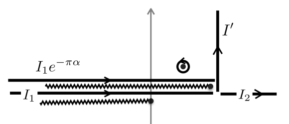
Figure 8: Contour for the integral Eq. (41).

From Eq. (29), $x<0$ has finite contribution for $\omega>0$, and with this the first exponential factor decays as we enclose the $\omega^{\prime}$-contour in the upper-half-plane. To obtain the integral (43) we organize the integral contour as shown in FIG. 8. The desired integral is $I_{1}+I_{2}$. The integral $I_{2}$ can be rotated to $I^{\prime}$ which converges much faster than $I_{2}$ due to the exponentially decaying factor in ${\rm e}^{-{\rm i}E/(2v_{0})(x^{2}+2x\omega^{\prime}/E)}$ for $x<0$ and $\omega^{\prime}={\rm i}y$ ($y>0$). The integral above the contour $C_{2}$ with the contribution $I_{1}{\rm e}^{\pi\alpha}$ combines with $I^{\prime}$ to give the residue integral at $\omega^{\prime}=\omega+{\rm i}\Gamma$,

$$I_{1}{\rm e}^{-\pi\alpha}+I^{\prime}=-({\rm i}/v_{0})\rho_{++}(0,x;\omega+{\rm i}\Gamma).$$ (94)

Therefore $G^{r}_{++}(0,x;\omega)$ can be expressed as

$${\rm e}^{\pi\alpha}[-({\rm i}/v_{0})\rho_{++}(0,x;\omega+{\rm i}\Gamma)-I^{\prime}]+I^{\prime}.$$ (95)

The term proportional to the residue becomes

$$-\frac{{\rm i}}{v_{0}}{\rm e}^{-\frac{{\rm i}E}{2v_{0}}(x^{2}+\frac{2x(\omega+{\rm i}\Gamma)}{E})}\left|\frac{\omega+{\rm i}\Gamma}{\omega-E|x|+}\right|^{-{\rm i}\alpha/2}{\rm e}^{-\alpha\varphi/2}.$$ (96)

The remaining term $({\rm e}^{\pi\alpha}-1)I^{\prime}$ can be easily evaluated due to the contour rotation in $I^{\prime}$,

$$\int_{0}^{\infty}\frac{{\rm e}^{-|x|y}\left|\frac{E|x|+{\rm i}y}{{\rm i}y}\right|^{-{\rm i}\alpha/2}{\rm e}^{\alpha/2(\tan^{-1}(y/E|x|)-\pi/2)}}{\omega-E|x|+{\rm i}y+{\rm i}\Gamma}\frac{{\rm i}{\rm d}y}{2\pi},$$ (97)

whose integral range is set by $|x|^{-1}$ and the integral is then well approximated by

$$\frac{-{\rm i}{\rm e}^{-\pi\alpha/4}}{2\pi(E|x|-\omega)|x|}(Ex^{2})^{-{\rm i}\alpha/2}\Gamma\left(1+{\rm i}\frac{\alpha}{2}\right).$$ (98)

In the small damping and $\alpha$ limit, the residue contribution dominates $({\rm e}^{\pi\alpha}-1)I^{\prime}$ and we arrive at Eq. (43).

Appendix C Small-Field Approximation

In the limit of large $\alpha$ with $E\ll\Delta$, approximating the retarded GF by that of zero-field limit may be a reasonable approximation. The justification of this idea is discussed further in the next section. The calculation of the lesser GF, however, is done with the full nonequilibrium Dyson’s equation (29). The zero-field retarded GF can be written down in the A/B sublattice basis as

$${\bf G}^{r}(\omega,p)=\left(\begin{array}[]{cc}\omega+\Delta+{\rm i}\Gamma&-v_{0}p\\ -v_{0}p&\omega-\Delta+{\rm i}\Gamma\end{array}\right)^{-1},$$ (99)

with the momentum $p$. Therefore, the retarded GF on the $A$-sublattice is given as

$$G^{r}_{AA}(x,\omega) = \int_{-\infty}^{\infty}\frac{(\omega-\Delta+{\rm i}\Gamma){\rm e}^{{\rm i}px}}{(\omega+{\rm i}\Gamma)^{2}-\Delta^{2}-v_{0}^{2}p^{2}}\frac{dp}{2\pi}$$

$$= -\frac{{\rm i}}{2v_{0}^{2}}\frac{\omega-\Delta+{\rm i}\Gamma}{k_{1}+{\rm i}k_{2}}{\rm e}^{{\rm i}k_{1}x-k_{2}|x|},$$

$$G^{r}_{AB}(x,\omega) = \frac{{\rm i}}{2v_{0}}{\rm e}^{{\rm i}k_{1}x-k_{2}|x|},$$ (100)

with

$$v_{0}k_{2} = \left[\left(u^{2}+\omega^{2}\Gamma^{2}\right)^{1/2}-u\right]^{1/2}$$

$$v_{0}^{2}k_{1}k_{2} = \omega\Gamma\mbox{ and }u=(\omega^{2}-\Delta^{2}-\Gamma^{2})/2.$$ (101)

Then, the local lesser GF at $x=0$, Eq. (29), is rewritten a

$$G^{<}_{AA}(\omega)=2{\rm i}\Gamma\int_{-\infty}^{-\omega/E}\left[|G^{r}_{AA}(x,\omega)|^{2}+|G^{r}_{AB}(x,\omega)|^{2}\right]{\rm d}x.$$ (102)

After straightforward calculations, one obtains

$$G^{<}_{AA}(\omega) = {\rm i}\frac{(\omega-\Delta)k_{1}+\Gamma k_{2}}{v_{0}^{2}(k_{1}^{2}+k_{2}^{2})}f(\omega)$$ (103)

$$= 2{\rm i}\pi\left(-\frac{1}{\pi}\mbox{Im }G^{r}_{AA}(0,\omega)\right)f(\omega)$$

with the distribution function

$$f(\omega) = \frac{1}{2}\exp\left(-\frac{2k_{2}(\omega)\omega}{E}\right)\Theta(\omega)$$ (104)

$$+ \left[1-\frac{1}{2}\exp\left(\frac{2k_{2}(\omega)\omega}{E}\right)\right]\Theta(-\omega).$$

The distribution function assumes the same form as the free 1-$d$ model, Eq. (15) with the inverse penetration depth $k_{2}(\omega)$ replacing $\Gamma$. In the $\Delta\to 0$ limit, $k_{2}$ becomes $\Gamma$. With a finite field with $|\omega|<\Delta$, the gap acts like a potential barrier and the wavefunction decays under the gap with the rate proportional to $\Delta$, leading to $k_{2}(\omega)\simeq\Delta/v_{0}$. Therefore the distribution function and the retarded GF are expected to behave as

$$f(\omega) \simeq \frac{1}{2}{\rm e}^{-2\Delta\omega/v_{0}E}$$

$$-\frac{1}{\pi}\mbox{Im }G^{r}_{AA}(0) = \frac{1}{2\pi v_{0}^{2}}\frac{\Gamma}{k_{2}}=\frac{\Gamma}{2\pi v_{0}\Delta}$$ (105)

for $0<\omega\lesssim\Delta$ in the large $\alpha$ limit, as verified in FIG. 2.

For the gap equation, the order parameter is calculated self-consistently as

$$\Delta = \frac{U}{2}(n_{A}-n_{B})$$ (106)

$$= \frac{U}{2}\int[G^{<}_{AA}(\omega;\Delta)-G^{<}_{AA}(\omega;-\Delta)]\frac{{\rm d}\omega}{2\pi{\rm i}}$$

$$= -\Delta\frac{U}{2\pi v_{0}}\int\frac{k_{1}f(\omega)}{v_{0}(k_{1}^{2}+k_{2}^{2})}{\rm d}\omega.$$

Appendix D Off-Diagonal Green’s Functions

The spectral function of the off-diagonal retarded GFs $G^{r}_{+-}(0,0;\omega)+G^{r}_{-+}(0,0;\omega)$, responsible for the gap equation, is given from Eq. (28) in the small $\Gamma$ limit as

$$2{\rm Re}\left\{\phi_{+}^{R}(0,\omega)[\phi_{-}^{R}(0,\omega)]^{*}-\phi_{+}^{R}(0,-\omega)[\phi_{-}^{R}(0,-\omega)]^{*}\right\}$$ (107)

after using the symmetry relations Eq. (38). This spectral function is purely real and odd in $\omega$. In the small-$\omega$ limit, the exact definition of the wavefunction (35) and (37) with Eq. (90) can be used to expand the spectral function in the lowest order of $\omega$ as

$$-\frac{2\sqrt{2}}{3}\frac{\Delta{\rm e}^{-\pi\alpha}}{(v_{0}E)^{2}}\omega^{3}\mbox{ for }\omega\simeq 0.$$ (108)

with the spectral weight suppressed by the LZ factor inside the gap.

In the large-$\omega$ limit, the asymptotic expansion (39) can be used to evaluate the GF. The wavefunction $\phi_{\pm}^{R}(0,\omega)$ consists of three contributions away from $\omega=0$: incoming, transmitted and reflected waves. For instance, for $\omega>0$ $\phi_{+}^{R}(0,\omega)$ has the transmitted wave. Due to the oscillation ${\rm e}^{\pm{\rm i}y^{2}}$ in Eq. (39) induced by the external field, the product between the wavefunction components may have cancelled or strong phase oscillations. For example, a product of incoming waves in $\phi_{+}^{R}(0,-\omega)$ and $\phi_{-}^{R}(0,-\omega)$ of Eq. (107) has the most dominant contribution that has cancelled phases. Cross-component products have uncancelled phases as ${\rm e}^{\pm{\rm i}\omega^{2}/v_{0}E}$. The oscillations become more rapid for smaller electric field. Such strong oscillation present in both frequency $\omega$ and position $x$ makes the numerical calculations quite challenging at small fields.

Analytic calculation for the non-oscillatory contribution at $|\omega|\gtrsim\Delta$ gives the approximate expression Gradshteyn and Rhizyk (2007)

$$-\frac{\Delta}{\omega}\left(1+\frac{\Delta^{2}}{2\omega^{2}}\right)\mbox{ for }|\omega|\gtrsim\Delta\mbox{ and }\frac{\Delta^{2}}{v_{0}E}\gtrsim 1,$$ (109)

which is, except for the prefactor $\Delta$, the same as the large-$\omega$ expansion of $(\omega^{2}-\Delta^{2})^{-1/2}$ in the gap equation (60). It is remarkable that the non-oscillatory part of the integral is independent of the electric field. FIG. 9 shows the the zero-field retarded GF (blue) threads the center of oscillation of the numerically accurate retarded GF (green). Although the integration of the oscillatory part is non-zero, especially with the important contribution close to $|\omega|\sim\Delta$, the approximation by the zero-field retarded GF is reasonable.

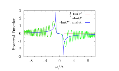
Figure 9: Off-diagonal GFs $G^{r,<}_{+-}(\omega)+G^{r,<}_{-+}(\omega)$ at $\Delta=\Delta_{\rm IMT}$, $E=E_{\rm IMT}$ and $\Gamma=0.01$. Fully numerical calculations for the lesser (red) and retarded (green) GFs show strong oscillation in frequency. The center of oscillation is well described by the analytic evaluation (blue) of the non-oscillatory part in the zero-field GF.

Appendix E Switching Field at the MIT

The on-set of the MIT is determined by the stability of the $\Delta=0$ solution in Eq. (54), the condition that the slope of the rhs remains below 1. Therefore the condition for the MIT is

$$\frac{1}{U}=\lim_{\Delta\to 0}\frac{1}{\Delta}\int\left[G^{<}_{-+}(\omega)+G^{<}_{+-}(\omega)\right]\frac{{\rm d}\omega}{2\pi{\rm i}}.$$ (110)

We can evaluate this exactly by using the first-order expansion of the GF out of the non-interacting GF considered in Section II.1. The retarded GF satisfies

$$(\omega+{\rm i}\Gamma-\hat{H}_{0}){\bf G}^{r}(x,x^{\prime})=\delta(x-x^{\prime}){\bf I},$$ (111)

with the GF matrix $({\bf G}^{r})_{ab}=G^{r}_{ab}$. $\hat{H}_{0}$ acts on the $x$. Taking the first-order expansion gives

$$\Delta G^{r,0}_{++}(x,x^{\prime})+(\omega+{\rm i}\Gamma-{\rm i}v_{0}\partial+Ex)G^{r}_{-+}(x,x^{\prime})=0.$$ (112)

Here, we suppressed $\omega$ in the expression for brevity. The unperturbed GF $G^{r,0}_{++}(x,x^{\prime})$ is given in Eq. (18) with $\lambda=+$. Defining $g(x,x^{\prime})={\rm e}^{{\rm i}\varphi(x,x^{\prime})-(\Gamma/v_{0})|x-x^{\prime}|}G^{r}_{-+}(x,x^{\prime})$, one solves the differential equation to obtain for $x>x^{\prime}$ as

$$g(x,x^{\prime})=g_{0}(x^{\prime})-\frac{\Delta}{v_{0}^{2}}\int_{x^{\prime}}^{x}{\rm e}^{2{\rm i}\varphi(y,x^{\prime})-2(\Gamma/v_{0})(y-x^{\prime})}{\rm d}y$$ (113)

with an arbitrary function $g_{0}(x^{\prime})$. Since $g(x,x^{\prime})\to 0$ as $|x-x^{\prime}|\to\infty$, one sets the boundary condition as

$$g(x,x^{\prime})=\frac{\Delta}{v_{0}^{2}}\int^{\infty}_{x}{\rm e}^{-2(\Gamma/v_{0})(y-x^{\prime})+2{\rm i}\varphi(y,x^{\prime})}{\rm d}y.$$ (114)

This gives us for $x<0$

$$G^{r}_{-+}(0,x)=\frac{\Delta}{v_{0}^{2}}{\rm e}^{(\Gamma/v_{0})x+{\rm i}\varphi(0,x)}\int_{0}^{\infty}{\rm e}^{-2(\Gamma/v_{0})y+2{\rm i}\varphi(y,0)}{\rm d}y,$$ (115)

and

$$G^{r}_{-+}(0,x)G^{r,0}_{++}(0,x)^{*}={\rm i}\frac{\Delta}{v_{0}^{3}}\Theta(-x){\rm e}^{2(\Gamma/v_{0})x}I(\omega,\Gamma,E),$$ (116)

with the integral denoted as $I(\omega,\Gamma,E)$. Performing an integral over $x$ in Eq. (29), we get

$$v_{0}^{2}G^{<}_{-+}(\omega)/\Delta=-I(\omega,\Gamma,E)\times\left\{\begin{array}[]{ll}{\rm e}^{-2\Gamma\omega/v_{0}E}&\omega>0\\ 1&\omega<0\end{array}\right..$$

Similarly one obtains

$$v_{0}^{2}G^{<}_{+-}(\omega)/\Delta=-I(\omega,\Gamma,-E)\times\left\{\begin{array}[]{ll}0&\omega>0\\ 1-{\rm e}^{-2\Gamma\omega/v_{0}E}&\omega<0\end{array}\right..$$

The integral $I(\omega,\Gamma,E)$ can be transformed to the parabolic cylinder function $D_{-1}(z)$ with $z=\sqrt{2/v_{0}E}{\rm e}^{-{\rm i}\pi/4}(\omega+{\rm i}\Gamma)$ by rotating the integration contour, and then approximated by the asymptotic expansion as

$$\frac{{\rm i}v_{0}}{2(\omega+{\rm i}\Gamma)}+\Theta(-\omega)\frac{{\rm e}^{{\rm i}\pi/4}}{\sqrt{E/\pi v_{0}}}\exp\left[\frac{-{\rm i}(\omega+{\rm i}\Gamma)^{2}}{v_{0}E}\right].$$ (117)

$I(\omega,\Gamma,-E)$ can be obtained by replacing $E\to{\rm e}^{{\rm i}\pi}E$ and $\Theta(-\omega)\to\Theta(\omega)$. The second term is highly oscillatory and we ignore its integral in the analytic estimate. It also shows that the oscillation goes like ${\rm e}^{-{\rm i}\omega^{2}/v_{0}E}$ for large $\omega$ and why the numerical calculation becomes problematic in the small $E$ limit. Then the first term is nothing but the zero-field retarded GF. Combining the results, we arrive at the MIT condition

$$\frac{2\pi v_{0}}{U}=-\int^{D}_{-D}\frac{\omega f^{0}_{\rm eff}(\omega)}{\omega^{2}+\Gamma^{2}}{\rm d}\omega$$ (118)

with the non-interacting distribution function Eq. (15). Performing this integral in a similar manner as considered in the main text, we obtain the integral

$$\int_{0}^{D}\frac{\omega{\rm d}\omega}{\omega^{2}+\Gamma^{2}}-\int_{0}^{\infty}\frac{\omega{\rm e}^{-2\Gamma\omega/v_{0}E}{\rm d}\omega}{\omega^{2}+\Gamma^{2}}\simeq\ln\left(\frac{2{\rm e}^{\gamma}\Gamma D}{v_{0}E}\right)$$ (119)

in the limit $\Gamma\ll T_{\rm eff}\sim v_{0}E/\Gamma\ll D$. This analytic expression agrees very well with the exact value by numerically evaluating $I(\omega,\Gamma,E)$ within 5% for the parameters considered. We then have the MIT condition at the switching field $E_{\rm MIT}$ as

$$E_{\rm MIT}\simeq{\rm e}^{\gamma}\frac{\Gamma}{v_{0}}\Delta_{0}\approx 1.78\,\frac{\Gamma}{v_{0}}\Delta_{0},$$ (120)

which gives, with the parameters used in this work, the analytic estimate $E_{\rm MIT}=0.0053$ at about 20% overestimate from the numerical value.

References

- Janod et al. (2015) E. Janod, J. Tranchant, B. Corraze, M. Querré, P. Stoliar, M. Rozenberg, T. Cren, D. Roditchev, V. T. Phuoc, M.-P. Besland, and L. Cario, Adv. Func. Mater. 25, 6287 (2015).
- Stoliar et al. (2013) P. Stoliar, L. Cario, E. Janod, B. Corraze, C. Guillot-Deudon, S. Salmon-Bourmand, V. Guiot, J. Tranchant, and M. Rozenberg, Adv. Mater. 25, 3222 (2013).
- Lee et al. (2015) J. S. Lee, S. Lee, and T. W. Noh, Appl. Phys. Rev. 2, 031303 (2015).
- Ridley (1963) B. K. Ridley, Proc. Phys. Soc. 82, 954 (1963).
- (5) P. Stoliar, J. Tranchant, B. Corraze, E. Janod, M. Besland, F. Tesler, M. Rozenberg, and L. Cario, Advanced Functional Materials 27, 1604740.
- Dubson et al. (1989) M. A. Dubson, Y. C. Hui, M. B. Weissman, and J. C. Garland, Phys. Rev. B 39, 6807 (1989).
- Driscoll et al. (2012) T. Driscoll, J. Quinn, M. Di Ventra, D. N. Basov, G. Seo, Y.-W. Lee, H.-T. Kim, and D. R. Smith, Phys. Rev. B 86, 094203 (2012).
- Guiot et al. (2013) V. Guiot, L. Cario, E. Janod, B. Corraze, V. T. Phuoc, M. Rozenberg, P. Stoliar, T. Cren, and D. Roditchev, Nat. Comm. 4, 1722 (2013).
- Aoki et al. (2014) H. Aoki, N. Tsuji, M. Eckstein, M. Kollar, T. Oka, and P. Werner, Rev. Mod. Phys. 86, 779 (2014).
- Datta (1995) S. Datta, Electronic Transport in Mesoscopic Systems (Cambridge University Press, Cambridge, UK, 1995).
- Jager et al. (2017) M. F. Jager, C. Ott, P. M. Kraus, C. J. Kaplan, W. Pouse, R. E. Marvel, R. F. Haglund, D. M. Neumark, and S. R. Leone, Proc. Nat. Aca. Sci. 114, 9558 (2017).
- Kemper et al. (2017) A. F. Kemper, M. A. Sentef, B. Moritz, T. P. Devereaux, and J. K. Freericks, Annalen der Physik 529, 1600235 (2017).
- Mitra et al. (2006) A. Mitra, S. Takei, Y. Kim, and A. Millis, Phys. Rev. Lett. 97 (2006).
- Mitra and Millis (2008) A. Mitra and A. Millis, Phys. Rev. B 77, 220404 (2008).
- Li et al. (2015) J. Li, C. Aron, G. Kotliar, and J. E. Han, Phys. Rev. Lett. 114, 226403 (2015).
- Mayer et al. (2015) B. Mayer, C. Schmidt, A. Grupp, J. Bühler, J. Oelmann, R. E. Marvel, R. F. Haglund, T. Oka, D. Brida, A. Leitenstorfer, and A. Pashkin, Phys. Rev. B 91, 457 (2015).
- Mazza et al. (2016) G. Mazza, A. Amaricci, M. Capone, and M. Fabrizio, Phys. Rev. Lett. 117, 176401 (2016).
- Zimmers et al. (2013) A. Zimmers, L. Aigouy, M. Mortier, A. Sharoni, S. Wang, K. G. West, J. G. Ramirez, and I. K. Schuller, Phys. Rev. Lett. 110, 056601 (2013).
- Guénon et al. (2013) S. Guénon, S. Scharinger, S. Wang, J. G. Ramirez, D. Koelle, R. Kleiner, and I. K. Schuller, Europhys. Lett. 101, 57003 (2013).
- Duchene et al. (1971) J. Duchene, T. M, P. Pailly, and G. Adam, Appl. Phys. Lett. 19, 115 (1971).
- Singh et al. (2015) S. Singh, G. Horrocks, P. M. Marley, Z. Shi, S. Banerjee, and G. Sambandamurthy, Phys. Rev. B 92, 155121 (2015).
- Aron (2012) C. Aron, Phys. Rev. B 86, 085127 (2012).
- Lee and Park (2014) W.-R. Lee and K. Park, Phys. Rev. B 89, 205126 (2014).
- Oka et al. (2003) T. Oka, R. Arita, and H. Aoki, Phys. Rev. Lett. 91, 66406 (2003).
- Oka and Aoki (2005) T. Oka and H. Aoki, Phys. Rev. Lett. 95, 137601 (2005).
- Li et al. (2017) J. Li, C. Aron, G. Kotliar, and J. E. Han, Nano Lett. 17, 2994 (2017).
- Sugimoto et al. (2008) N. Sugimoto, S. Onoda, and N. Nagaosa, Phys. Rev. B 78, 155104 (2008).
- Kim et al. (2010a) H.-T. Kim, B.-J. Kim, S. Choi, B.-G. Chae, Y.-W. Lee, T. Driscoll, M. M. Qazilbash, and D. N. Basov, J. Appl. Phys. 107, 023702 (2010a).
- Kim et al. (2010b) J. Kim, C. Ko, A. Frenzel, S. Ramanathan, and J. E. Hoffman, Applied Physics Letters 96, 213106 (2010b).
- Han (2013) J. E. Han, Phys. Rev. B 87, 085119 (2013).
- Han and Li (2013) J. E. Han and J. Li, Phys. Rev. B 88, 075113 (2013).
- Schwinger (1951) J. Schwinger, Phys. Rev. 82, 664 (1951).
- Zener (1932) C. Zener, Proc. R. Soc. A 137, 696 (1932).
- Whittaker and Watson (1920) E. T. Whittaker and G. N. Watson, A Course of Modern Analysis (University Press, Cambridge, 1920).
- Gradshteyn and Rhizyk (2007) I. S. Gradshteyn and I. M. Rhizyk, Table of Integrals, Series, and Products (Elsevier, New York, 2007).
- Eckstein et al. (2010) M. Eckstein, T. Oka, and P. Werner, Phys. Rev. Lett. 105, 146404 (2010).
- Eckstein and Werner (2011) M. Eckstein and P. Werner, Phys. Rev. Lett. 107, 186406 (2011).
- Slater (1951) J. C. Slater, Phys. Rev. (1951).
- Doron et al. (2016) A. Doron, I. Tamir, S. Mitra, G. Zeltzer, M. Ovadia, and D. Shahar, Phys. Rev. Lett. 116, 951 (2016).
- Wu et al. (2011) T.-L. Wu, L. Whittaker, S. Banerjee, and G. Sambandamurthy, Phys. Rev. B 83, 073101 (2011).
- Kirillov (1994) A. N. Kirillov, arXiv.org (1994), hep-th/9408113 .
- Altshuler et al. (2009) B. Altshuler, V. Kravtsov, I. Lerner, and I. Aleiner, Phys. Rev. Lett. 102, 176803 (2009).
- Martin et al. (1973) P. C. Martin, E. D. Siggia, and H. A. Rose, Phys. Rev. A 8, 423 (1973).
- Schmittmann and Zia (1995) B. Schmittmann and R. K. P. Zia, Statistical Mechanics of Driven Diffusive Systems (Academic Press, San Diego, 1995).