Robust Hadamard matrices,
unistochastic rays in Birkhoff polytope
and equi-entangled bases in composite spaces

Abstract

We study a special class of (real or complex) robust Hadamard matrices, distinguished by the property that their projection onto a $2$-dimensional subspace forms a Hadamard matrix. It is shown that such a matrix of order $n$ exists, if there is a skew Hadamard matrix of a symmetric conference matrix of this size. This is the case for any even $n\leq 20$, and for these dimensions we demonstrate that a bistochastic matrix $B$ located at any ray of the Birkhoff polytope, (which joins the center of this body with any permutation matrix), is unistochastic. An explicit form of the corresponding unitary matrix $U$, such that $B_{ij}=|U_{ij}|^{2}$, is determined by a robust Hadamard matrix. These unitary matrices allow us to construct a family of orthogonal bases in the composed Hilbert space of order $n\times n$. Each basis consists of vectors with the same degree of entanglement and the constructed family interpolates between the product basis and the maximally entangled basis. In the case $n=4$ we study geometry of the set ${\mathcal{U}}_{4}$ of unistochastic matrices, conjecture that this set is star-shaped and estimate its relative volume in the Birkhoff polytope ${\mathcal{B}}_{4}$.

Dedicated to the memory of Uffe Haagerup (1949-2015)

1 Introduction

Hadamard matrices with a particular structure attract a lot of attention, as their existence is related to several problems in combinatorics and mathematical physics. Usually one poses a question, whether for a given size $n$ there exists a Hadamard matrix with a certain symmetry or satisfying some additional conditions. Such a search for structured Hadamard matrices can be posed as well in the standard case of real Hadamard matrices [16], or in the more general complex case [10, 29, 28].

To simplify investigations one studies equivalence classes of Hadamard matrices, which differ only by permutations of rows and columns and by multiplication by diagonal unitary matrices. It was shown by Haagerup [15] that for dimensions $n=2,3$ and $n=5$ all complex Hadamard matrices are equivalent while for $n=4$ there exists a one parameter family of inequivalent matrices.

In the recent paper by Karlsson [19], aimed to construct new families of complex Hadamard matrices of size $n=6$, the author studied $H_{2}$-reducible matrices defined as Hadamard matrices with the property that all their blocks of size $2$ form Hadamard matrices.

In this work we introduce a related, but different notion of robust Hadamard matrices. This class contains a Hadamard matrix $H_{n}$, such that each of its principal minors of order two forms a Hadamard matrix $H_{2}$. The name refers to the fact that the Hadamard property is robust with respect to projection, as any projection of $H_{n}$ onto a two dimensional subspace spanned by the elements of the standard basis is a Hadamard matrix.

The notion of robust Hadamard matrices will be useful to broaden our understanding of the problem of unistochasticity inside the Birkhoff polytope [6]. For any bistochastic matrix $B$ one asks whether there exist a unitary matrix $U$, such that $B_{ij}=|U_{ij}|^{2}$. In the simplest case $n=2$ any bistochastic matrix is unistochastic, for $n=3$ the necessary and sufficient conditions for this property are known [3, 17, 23], in order $n=4$ we provide an explicit construction in Appendix A, while for $n\geq 5$ the unistochasticity problem remains open [1, 5].

A robust Hadamard matrix $H_{n}$ will be used to to find unitary matrices of order $n$, designed to prove unistochasticity of bistochastic matrices located at any ray of the Birkhoff polytope. The key idea behind this construction – a decomposition of bistochastic matrix of an even dimension into square blocks of size two – was used in the algorithm of Haagerup to analyze the unistochasticity problem for $n=4$. A family of unistochastic matrices joining a permutation matrix with the flat bistochastic matrix $W_{n}$ of van der Waerden allows us to construct a family of orthogonal bases in the composed Hilbert space ${\mathcal{H}}_{n}\otimes{\mathcal{H}}_{n}$, which contains equi-entangled vectors and interpolates between the product basis and the maximally entangled basis [30]. Although such "equi-entangled bases" have already appeared in the literature [14, 18], the present construction is simpler as it corresponds to straight lines in the Birkhoff polytope ${\mathcal{B}}_{n}$.

This work is organized as follows. In Section 2 we review the necessary notions, introduce robust Hadamard matrices and demonstrate their existence if skew Hadamard matrices or symmetric conference matrices exist. In Section 3 we present the unistochasticity problem and show how robust Hadamard matrices can be used to prove unistochasticity of bistochastic matrices at a ray joining the center of the Birkhoff polytope with any of its corners. The notion of complementary permutation matrices is used in Section 4 to demonstrate unistochasticity of certain subsets of the Birkhoff polytope of an even dimension $n$ for which robust Hadamard matrices exist. Unitary matrices of an even order $n\leq 20$ corresponding to rays in the Birkhoff polytope are applied to construct in Section 5 a family of equi-entangled bases for the composite systems of size $n\times n$. In Section 6 we analyze the unistochasticity problem for $n=4$: using the Haagerup procedure, presented in Appendix A, we investigate the geometry of the set $\mathcal{U}_{4}$ of unistochastic matrices of order $n=4$. An estimation of the relative volume of the set $\mathcal{U}_{4}$ with respect to the standard Lebesgue measure is presented in Appendix B. In Appendix C it is shown that robust Hadamard matrices do not exists for $n=3$ and $n=5$, while extensions of these results for any odd $n$, suggested by the referee, are presented in Appendix D.

2 Robust Hadamard Matrices

We are going to discuss various subclasses of the set of Hadamard matrices. Let us start with basic definitions. Let $M_{n}(\mathbb{R})$ and $M_{n}(\mathbb{C})$ denote set of all real (complex) matrices of order $n$.

In analogy to the standard notion of (real) Hadamard matrices one defines [10, 29] complex Hadamard matrices.

Definition 2.1.

Matrices of order $n$ with unimodular entries, unitary up to a scaling factor,

$$\mathcal{H}(n)=\{H\in M_{n}(\mathbb{C}):\,(HH^{*}=n\mathbb{I},|H_{ij}|=1,i,j=1,\dots,n)\},$$

are called Hadamard matrices. If all entries of the matrix $H$ are real, it is called a real Hadamard.

Definition 2.2.

Set of robust Hadamard matrices for dimension $n$

$$\mathcal{H}^{R}(n)=\mathcal{f}H\in M_{n}(\mathbb{C}):\,\forall_{i,j\in 1,2,...,n,\,i\neq j}\begin{pmatrix}H_{ii}&H_{ij}\\ H_{ji}&H_{jj}\end{pmatrix}\in\mathcal{H}_{\mathbb{C}}(2)\}.$$

The name refers to the fact that the Hadamard property is robust with respect to projections: $H^{R}$ remains Hadamard after a projection $\Pi_{2}$ onto a subspace spanned by two vectors of the basis used, $\Pi_{2}H^{R}\Pi_{2}\in\mathcal{H}(2)$.

Robust Hadamard matrices of order $n$ will be denoted by $H^{R}_{n}$ or $H^{R}$. Equivalent definition is:

Robust Hadamard matrix is a Hadamard matrix, in which all principal minors of order two are extremal so that their modulus is equal to 2.

The notion of Hadamard matrices robust with respect to projection can also be used in the complex case.

2.1 Equivalence relations

Let ${\mathcal{P}}(n)$ or $\mathcal{P}$ denote the set of all permutation matrices $P$ of order $n$. Permutation matrices are used to introduce the following equivalence relation in the set of Hadamard matrices.

Definition 2.3.

Two Hadamard matrices are called equivalent, written $H_{1}\sim H_{2}$, if there exist unitary diagonal matrices $D_{1},\,D_{2}$ and permutation matrices $P_{1},\,P_{2}\in\mathcal{P}$ such that

$$H_{1}\sim H_{2}=P_{1}D_{1}H_{1}D_{2}P_{2}.$$ (2.1)

In dimensions $1,2,4,8$ and $12$ all real Hadamard matrices are equivalent. For $n=16$ there exist five equivalence classes [16] and this number grows fast [24] with $n$. It is also convenient to distinguish a finer notion of equivalence with respect to signs.

Definition 2.4.

Two Hadamard matrices are equivalent with respect to signs, written $H_{1}\approx H_{2}$, if one is obtained from the other by negating rows or columns,

$$H_{1}\approx H_{2}=D_{1}H_{1}D_{2},$$

where $D_{1},\,D_{2}$ are orthogonal diagonal matrices.

By definition, if $H_{1}\approx H_{2}$ then $H_{1}\sim H_{2}$.

2.2 Basic properties of robust Hadamard matrices

Some basic properties of robust Hadamard matrices are:

• By construction every $H_{2}$ is robust;   $\mathcal{H}(2)\equiv\mathcal{H}^{R}(2)$.

• For $n\geq 4$ not every $H$ is robust;   $\mathcal{H}(n)\neq\mathcal{H}^{R}(n),\,n\geq 4$.

• If $H$ is robust then its transpose $H^{T}$ is also robust.

• Real robust matrices form sign-equivalence classes within the real Hadamard equivalence classes. Thus, for the orders with one equivalence class ($n=1,2,4,8,12$) all real robust matrices are equivalent.

2.3 Skew Hadamard and robust Hadamard matrices

Definition 2.5.

A real Hadamard matrix $H$ is a skew Hadamard matrix, written $H\in\mathcal{H}^{S}(n)$, if and only if:

$$H+H^{T}=2\mathbb{I}.$$

Lemma 2.6.

Every skew Hadamard matrix is robust Hadamard.

Proof.

By definition, every diagonal element of a skew Hadamard matrix $H$ is equal to $1$. Furthermore, any pair of off–diagonal elements, with the number of row and column exchanged, consist of two entries with the opposite sign. Hence the determinant of every principal minor of order two is equal to $2$, which means that $H$ is a robust Hadamard. ∎

Lemma 2.7.

Any robust Hadamard matrix $H^{R}$ is sign-equivalent to a certain skew Hadamard matrix: $H^{S}\approx H^{R}$.

Proof.

To show this observe that by multiplying the columns of a robust Hadamard matrix $H^{R}$ which contain negative entries at the diagonal by $(-1)$ we obtain a skew matrix. Note that multiplication of columns does not take $H^{R}$ out of the set of robust Hadamard matrices. ∎

One can easily see that the following Hadamard matrix of order four is robust and is equivalent to a skew Hadamard:

$$H^{R}_{4}=\begin{pmatrix}1&1&1&1\\ 1&-1&-1&1\\ 1&1&-1&-1\\ 1&-1&1&-1\end{pmatrix}\approx H^{R,S}_{4}=\begin{pmatrix}1&-1&-1&-1\\ 1&1&1&-1\\ 1&-1&1&1\\ 1&1&-1&1\end{pmatrix}.$$

To show that the set of $H_{2}$-reducible matrices introduced by Karlsson [19] differs from the set $\mathcal{H}^{R}(n)$ of robust Hadamard matrices discussed here, consider the following matrix of size $n=4$,

$$\begin{pmatrix}1&1&1&1\\ 1&-1&1&-1\\ 1&1&-1&-1\\ 1&-1&-1&1\\ \end{pmatrix}.$$

It is easy to see that the above matrix is $H_{2}$-reducible but is not robust, so these two sets do differ.

2.4 Symmetric conference matrices and robust Hadamard matrices

Definition 2.8.

A symmetric matrix with entries $\pm 1$ outside the diagonal and $0$ at the diagonal, which satisfy orthogonality relations:

$$CC^{T}=(n-1)\mathbb{I},$$

is called a symmetric conference matrix.

Lemma 2.9.

Matrices of the structure:

$$H^{R}=C+i\mathbb{I},$$

where $C$ is symmetric conference matrix, are complex robust Hadamard matrices.

This statement holds as the determinant of any principal submatrix of $H^{R}$ or order two is equal to $-2$.

To establish whether for a given order $n$ there exists a robust Hadamard matrix it is therefore sufficient to find a skew Hadamard matrix or a symmetric conference matrix of size $n$. Concerning odd dimensions we show in Appendix C and D that robust Hadamard matrices do not exist for any odd $n$.

3 Robust Hadamard matrices and unistochasticity

Robust Hadamard matrices, introduced in the previous Section, will be used to investigate the problem, whether a given bistochastic matrix is unistochastic. Before demonstrating such an application let us recall the necessary notions.

3.1 Definitions

Definition 3.1.

The set $\mathcal{B}_{n}$ of bistochastic matrices of size $n$ consists of matrices with non-negative entries which satisfy two sum conditions:

$$\mathcal{B}_{n}=\{B\in M_{n}(\mathbb{R}),\ \sum_{i=1}^{n}B_{ij}=\sum_{i=1}^{n}B_{ji}=1,\ j=1,\dots,n\}$$

.

Due to the Birkhoff theorem [6], the set $\mathcal{B}_{n}$ is equal to the convex hull of all permutation matrices of order $n$.

Definition 3.2.

A bistochastic matrix $B\in\mathcal{B}_{n}$ is called unistochastic if and only if there exists a unitary matrix $U\in U(n)$, $UU^{*}=\mathbb{I}$, such that

$$B_{ij}=|U_{ij}|^{2},\ i,j=1,2,\dots,n$$

Using the notion of the Hadamard product $\circ$ of two matrices one can say that $B$ is unistochastic, if there exist a unitary $U$ such that $B=U\circ{\bar{U}}$.

If matrix $U$ is orthogonal the matrix $B$ is called orthostochastic. The sets of all unistochastic and orthostochastic matrices of order $n$ will be denoted by $\mathcal{U}_{n}$ and $\mathcal{O}_{n}$, respectively. Above definitions imply:

$$\mathcal{O}_{n}\subset\mathcal{U}_{n}\subset\mathcal{B}_{n}.$$

3.2 In search for unistochasticity

It is easy to see that for $n=2$ all three sets coincide, $\mathcal{O}_{2}=\mathcal{U}_{2}=\mathcal{B}_{2}$. While conditions for unistochasticity are known [3, 11, 12] for $n=3$, the case $n\geq 4$ remains open – see [5]. Given an arbitrary bistochastic matrix $B$ of order $n$, it is easy to verify whether certain necessary conditions for unistochasticity are satisfied, but in general, no universal sufficient conditions are known and one has to rely on numerical techniques [5, 13].

Since we are looking for a unitary $U$ such that $B=U\circ{\bar{U}}$, the absolute value of each entry is fixed, $|U_{ij}|=\sqrt{B_{ij}}$, and one can investigate constraints implied by the unitarity. The scalar product of any two different columns of $U$ is given by a sum of $n$ complex numbers of the form $U_{ij}{\bar{U}}_{ij^{\prime}}$. This sum can vanish if the largest modulus is not larger than the half of the sum of all $n$ moduli. For $n=3$ this condition is equivalent to the triangle inequality. The above observation, allows one to obtain a set of necessary conditions, a bistochastic $B$ must satisfy to be unistochastic [26], related to orthogonality of columns,

$$\max_{m=1,\ldots,n}\sqrt{B_{mk}B_{ml}}~{}\leq~{}\frac{1}{2}\sum_{j=1}^{n}\sqrt{B_{jk}B_{jl}}\ ,{\rm~{}~{}for~{}~{}all~{}~{}}1\leq k<l\leq n,$$ (3.1)

and rows of $U$,

$$\max_{m=1,\ldots,n}\sqrt{B_{km}B_{lm}}~{}\leq~{}\frac{1}{2}\sum_{j=1}^{n}\sqrt{B_{kj}B_{lj}}\ ,{\rm~{}~{}for~{}~{}all~{}~{}}1\leq k<l\leq n\ .$$ (3.2)

We shall refer to the above relations as polygon inequalities or "chain" conditions: the longest link of a closed chain cannot be longer than the sum of all other links. For matrices of size $n=3$ these necessary conditions are known to be sufficient for unistochasticity [3, 23], while $B$ is orthostochastic if the bounds are saturated. Furthermore, in this dimension all chain conditions are equivalent – if inequality (3.1) is satisfied for any pair of two columns it will also be satisfied for the remaining pairs of columns and vectors [17, 11]. The case $n=4$ occurs to be more complicated as the chain inequalities are not sufficient [1, 5], and examples of bistochastic matrices are known for which these condition are satisfied for some pairs of columns or rows and not satisfied by the other pairs [25, 31]. An algorithm allowing one to establish numerically whether a given bistochastic matrix $B$ of order $n=4$ is unistochastic is described in the Appendix A.

Not being able to solve the unistochasticity problem in its full extent, we shall consider particular subsets of the Birkhoff polytope $\mathcal{B}_{n}$ of an arbitrary dimension $n$. Figure 1 presents a sketch of the set of bistochastic matrices visualizing the problems considered.

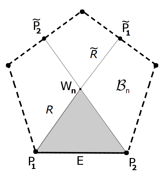
Figure 1: Sketch of the Birkhoff polytope $\mathcal{B}_{n}$ - a set of ${(n-1)^{2}}$ dimensions: the flat matrix $W_{n}$ in the center, permutation matrices $P_{i}$ at the corners. The corresponding rays $\mathcal{R}$ and counter-rays $\widetilde{\mathcal{R}}$ meet at $W_{n}$. The counter-ray $\widetilde{\mathcal{R}}$ ends at the counter-permutation matrix $\tilde{P}_{1}$ Bold lines denote complementary edges, while dashed lines represent non-complementary edges. Region in gray – the triangle $\Delta P_{1},P_{2},W_{n}$ – represents sets proved to be unistochastic.

Definition 3.3.

Bistochastic matrix $W_{n}$, in which every element is equal to $1/n$, is called the flat matrix.

Definition 3.4.

A one-dimensional set of bistochastic matrices obtained by a convex combination of the flat matrix $W_{n}$ and any permutation matrix $P$ is called a bistochastic ray,

$$\mathcal{R}_{n}=\{R_{\alpha}\in\mathcal{B}_{n}:\,R_{\alpha}=\alpha P+(1-\alpha)W_{n},\ P\in\mathcal{P}(n),\ \alpha\in[0,1]\}.$$ (3.3)

Definition 3.5.

A set $\widetilde{\mathcal{R}}_{n}$ of bistochastic matrices belonging to the line joining the flat matrix $W_{n}$ and a permutation matrix $P$, outside the segment $PW_{n}$ is called a counter-ray. These matrices can be expressed as pseudo-mixtures (3.3) with a negative weight $\alpha\in[-\frac{1}{n-1},0)$.

For $P=\mathbb{I}$, the family of matrices belonging to the ray is as follows

$$\mathcal{R}_{\mathbb{I}}=\Bigg{\{}R_{\alpha}=\begin{pmatrix}a&b&\ldots&b&b\\ b&a&\ldots&b&b\\ \vdots&\vdots&\ddots&\vdots&\vdots\\ b&b&\ldots&a&b\\ b&b&\ldots&b&a\end{pmatrix},a=\frac{(n-1)\alpha+1}{n};\text{ }b=\frac{1-a}{n-1};\text{ }\alpha\in[0,1]\Bigg{\}}.$$ (3.4)

3.3 Robust Hadamard matrices imply unistochasticity

Lemma 3.6.

If there exists a robust complex Hadamard matrix $H^{R}$ of order $n$ then all rays and counter-rays of the Birkhoff polytope $\mathcal{B}_{n}$ of order $n$ are unistochastic.

Proof.

First let us show, that for any robust Hadamard matrix ${H}^{R}$ the following property holds:

$${H}^{R}{D}^{*}+D{{H}^{R}}^{*}=2\mathbb{I},$$ (3.5)

where $D$ is the diagonal matrix containing diagonal entries of $H^{R}$. Diagonal elements of the left-hand side of eq. (3.5) are equal to $2H_{ii}H_{ii}^{*}=2$, while off-diagonal entries of this sum, $i\neq j$, read $H_{ij}{H_{jj}}^{*}+{H_{ji}}^{*}{H}_{ii}$. In order to evaluate these terms we shall use the fact that the matrix ${H}^{R}{D}^{*}\sim{H}^{R}$ is robust. Let $M_{2}$ be the principal submatrix of ${H}^{R}{D}^{*}$ of order two spanned by the rows $i$ and $j$. Since ${H}^{R}{D}^{*}$ is robust then $M_{2}\in\mathcal{H}_{\mathbb{C}}(2)$, so that $M_{2}M_{2}^{*}=2\mathbb{I}_{2}$. Writing down the entries of this matrix explicitly one obtains

$$M_{2}{M_{2}}^{*}=\begin{pmatrix}2&H_{ij}{H_{jj}}^{*}+{H_{ji}}^{*}{H}_{ii}\\ H_{ij}^{*}{H_{jj}}+{H_{ji}}{H}_{ii}^{*}&2\end{pmatrix}.$$

Since this matrix is proportional to identity its off-diagonal entries vanish, so that $H_{ij}{H_{jj}}^{*}+{H_{ji}}^{*}{H}_{ii}=0,$ for $i\neq j$. Hence equation (3.5) is shown to be true.

For any bistochastic matrix $R$ of order $n$ belonging to the ray $\mathcal{R}_{\mathbb{I}}$ or counter ray $\widetilde{\mathcal{R}}$ let us now construct a matrix $U$,

$$U=\sqrt{a}D+\sqrt{b}(H^{R}-D),$$

where real parameters $a$ and $b$ defined by eq. (3.4) satisfy the condition $(n-1)b+a=1$. Making use of these relations, definition  (2.1) and eq. (3.5) we get

$$UU^{*}=(\sqrt{b}H^{R}-(\sqrt{b}-\sqrt{a})D)(\sqrt{b}{H^{R}}^{*}-(\sqrt{b}-\sqrt{a}){D}^{*})=$$

$$bH^{R}{H^{R}}^{*}-\sqrt{b}(\sqrt{b}-\sqrt{a})(H^{R}{D}^{*}+D{H^{R}}^{*})+(\sqrt{b}-\sqrt{a})^{2}D{D}^{*}=((n-1)b+a)\mathbb{I}=\mathbb{I}.$$

This shows that the matrix $U$ is unitary. Since the matrix $R$ satisfies the relation $R_{ij}=|U_{ij}|^{2}$, it is unistochastic. Hence any matrix $R$ at any ray $\mathcal{R}$ of the Birkhoff polytope $\mathcal{B}_{n}$ or any counter-ray $\widetilde{\mathcal{R}}$ is unistochastic for any dimension $n$, for which a robust Hadamard matrix exists. ∎

In particular, if the robust Hadamard matrix is real, so that $U$ becomes orthogonal, then the matrix $R$ is orthostochastic. Since every skew Hadamard matrix is robust (lemma 2.6), we arrive at the following statements:

Proposition 3.7.

For every order $n$, for which there exists a symmetric conference matrix, every matrix belonging to any ray $\mathcal{R}$ or any counter-ray $\widetilde{\mathcal{R}}$ of the Birkhoff polytope $\mathcal{B}_{n}$ is unistochastic.

Proposition 3.8.

For any order $n$, for which there exists a skew Hadamard matrix $H^{S}$, every matrix belonging to any ray $\mathcal{R}$ or any counter-ray $\widetilde{\mathcal{R}}$ of the Birkhoff polytope $\mathcal{B}_{n}$ is orthostochastic.

Existence of skew Hadamard matrices for orders $n=4k$ is proved for $k<69$, proper construction was done by Paley. There are infinitely many cases of skew Hadamard matrices of higher orders [21].

It is known that for dimensions $n=6,10,14,18$ there exists a symmetric conference matrix [22]. However, for order $n=22$ there are no such matrices, since $21$ is not the sum of two squares.

Those facts imply the main result of this work:

Theorem 3.9.

For any even order $n\leq 20$ all rays and counter-rays of the Birkhoff polytope $\mathcal{B}_{n}$ are

1. orthostochastic (for $n=2,4,8,12,16,20$) or

2. unistochastic (for $n=6,10,14,18$).

Proof.

It is a simple conclusion from proposition 3.7 and proposition 3.8 which allow one for an explicit construction of the corresponding orthogonal and unitary matrices. ∎

Note that the above statement holds also for infinitely many dimensions, for which symmetric conference matrices are known (first found by Paley – see e.g. [16]).

4 Unistochasticity of certain triangles embedded inside Birkhoff polytope

A convex combination of any two permutation matrices forms an edge (or a diagonal) of the Birkhoff polytope $\mathcal{B}_{n}$,

$$E=\alpha P+(1-\alpha)Q$$

Au-Yeng and Cheng introduced the notion of complementary permutations [2].

Definition 4.1.

Let $P=(P_{ij})$ and $Q=(Q_{ij})$ be two permutation matrices. Then the matrices $P$ and $Q$ are called complementary if equality $P_{ij}=P_{hk}=Q_{ik}=1$ implies $Q_{hj}=1$ for all $i,j,h,k\in\{1,...,n\}$; (consequently, if $Q_{ij}=Q_{hk}=P_{ik}=1$ then $P_{hj}=1$).

Proposition 4.2.

If $P$ and $Q$ are two complementary permutation matrices then the entire edge $PQ$ of the Birkhoff polytope $\mathcal{B}_{n}$ connecting $P$ and $Q$ is orthostochastic. If $P$ and $Q$ are not complementary, then the edge is not unistochastic, besides the orthostochastic corners $P$ and $Q$.

Below we generalize above proposition, proved by Au-Yeng and Cheng [2] to establish unistochasticity of some sets of larger dimension. Let us first distinguish the following notion:

Definition 4.3.

Two permutation matrices $P$ and $Q$ will be called strongly complementary if they are complementary and if the condition $P_{ij}=1$ implies $Q_{ij}=0$.

In other words their non-zero elements are put in different places, so their Hadamard product vanishes, $P\circ Q=0$. Due to symmetry of $\mathcal{B}_{n}$ one can take the identity matrix for the permutation matrix $P$ without loosing generality. A matrix $Q$ is strongly complementary to $P=\mathbb{I}$ if and only if $Q$ is an involution, $Q^{2}=\mathbb{I}$, and every diagonal element of $Q$ is $0$. Due to complementarity, the dimension of $Q$ is even. Making use of the flat bistochastic matrix $W_{n}$ we can now formulate statements concerning triangles $\Delta(A,B,C)$ belonging to $\mathcal{B}_{n}$ and spanned by vertices $A$, $B$ and $C$.

Lemma 4.4.

Consider dimension $n$ for which a robust Hadamard matrix $H^{R}$ exists. If $P$ and $Q$ are strongly complementary permutation matrices, then the triangle $\Delta(P,Q,W_{n})$ is unistochastic. If $H^{R}$ is real then the triangle contains orthostochastic matrices.

Proof.

As before, we can restrict our attention to the case $P=\mathbb{I}$. Every matrix on the line connecting $\mathbb{I}$ and $Q$ can be written as:

$$\begin{pmatrix}b&a&0&0&\dots\\ a&b&0&0&\dots\\ 0&0&b&a&\dots\\ 0&0&a&b&\dots\\ \vdots&\vdots&\vdots&\vdots&\ddots&\\ \end{pmatrix},$$

where $a+b=1$. Thus, any bistochastic matrix belonging to the triangle $\Delta(P,Q,W_{n})$ reads

$$\begin{pmatrix}b&a&c&c&\dots\\ a&b&c&c&\dots\\ c&c&b&a&\dots\\ c&c&a&b&\dots\\ \vdots&\vdots&\vdots&\vdots&\ddots&\\ \end{pmatrix},$$

where $a+b+(n-2)c=1$. Taking the entry-wise square root of this matrix and multiplying it element-wise by a robust Hadamard matrix we obtain the corresponding unitary matrix, sufficient to show the desired property. ∎

This statement is visualized by a gray triangle of unistochastic matrices shown in Fig. 1. The above result can be generalized for a larger set of permutation matrices $\{P_{1},P_{2},...,P_{k}\}$ of dimension $n$, in which each pair of matrices is strongly complementary. Then an analogous reasoning shows that the bistochastic matrices belonging to $2$-faces of the polytope defined by the convex hull of $k$ these permutation matrices and the flat matrix $W_{n}$ are unistochastic.

Due to the definition of strong complementarity each pair of matrices has non-zero entries in different places, so that $k\leq n$. We are not able to determine how the maximal number $k$ of such matrices depends on the dimension $n$, nor whether the bistochastic matrices belonging to the interior of this polytope are unistochastic.

5 Equi-entangled bases

Any quantum system composed from two subsystems, with $n$ levels each, can be described in a Hilbert space with a tensor product structure. It is often natural to use the standard, product basis, usually denoted by $|k,m\rangle=|k\rangle\otimes|m\rangle$ with $k,m=1,\dots,n$. However, for certain problems it is advantageous to use bases consisting of maximally entangled states. In the simplest case of $n=2$ one uses the Bell basis consisting of four orthogonal states of size four, $|\Psi^{\pm}\rangle=(|0,0\rangle\pm|1,1\rangle)/\sqrt{2}$ and $|\Phi^{\pm}\rangle=(|0,1\rangle\pm|1,0\rangle)/\sqrt{2}$. These Bell states are also called maximally entangled, as their partial traces are maximally mixed. In this Section we follow the notation of [30], often used in quantum theory.

For any higher dimension $n$ such entangled bases were constructed by Werner [30]. A slightly more general variant of this construction discussed in [4] allows one to write a set of $n^{2}$ orthogonal states related to a given unitary matrix $U$ of order $n$. Making use of unistochastic matrices belonging at a ray of the Birkhoff polytope and determined by robust Hadamard matrices, we shall construct a family of bases interpolating between separable and maximally entangled basis.

Consider a unitary matrix $U$ of order $n$, associated with the unistochastic matrix $B=U\circ{\bar{U}}$, which belongs to the ray $R$ of the Birkhoff polytope ${\mathcal{B}}_{n}$ – see Fig. 1. It exists for all dimensions, for which a robust Hadamard matrix exists (i.e. for all even dimensions $n\leq 20$) and allows us to construct an equi-entangled orthogonal basis in the Hilbert space describing a composed system of size $n\times n$.

Proposition 5.1.

Let $|m,m^{\prime}\rangle$ with $m,m^{\prime}=1,\dots n$ form the standard computation basis in the bipartite Hilbert space of size $n\times n$. Let $U$ be a unitary matrix of order $n$, associated with the unistochastic matrix $B=U\circ{\bar{U}}$, which belongs to a ray $R$ of the Birkhoff polytope ${\mathcal{B}}_{n}$. Then the set of $n^{2}$ vectors in this space defined by

$$|\psi_{m,k}\rangle=\sum_{j=1}^{n}U_{mj}\;|j\rangle\otimes|j+k_{|{\rm mod}\ n}\rangle,\ \ k,m=1,\dots,n$$ (5.1)

a) forms an orthonormal basis;

b) the basis is equi-entangled, as all its elements have the same degree of entanglement.

Proof.

a) To show this property it is sufficient to check the scalar product

$$\langle\psi_{m,k}|\psi_{m^{\prime},k^{\prime}}\rangle=\sum_{j,j^{\prime}}U^{*}_{mj}\langle j,j+k_{|{\rm mod}\ n}|j^{\prime},j^{\prime}+k^{\prime}_{|{\rm mod}\ n}\rangle U_{m^{\prime}j^{\prime}}=\\ =\sum_{j,j^{\prime}}U^{*}_{jm}U_{m^{\prime}j^{\prime}}\delta_{k,k^{\prime}}\delta_{j,j^{\prime}}=\delta_{k,k^{\prime}}\sum_{j}U_{m^{\prime}j}U^{*}_{jm}=\delta_{k,k^{\prime}}\delta_{m,m^{\prime}}.$$ (5.2)

Due to unitarity of $U$ the orthogonality holds for any $k,k^{\prime},m,m^{\prime}=1,\dots,n$, which implies that the vectors (5.1) form an orthonormal basis.

b) To analyze the degree of entanglement we specify our considerations to a family $U(a)$ of unitary matrices given in  (3.4) and parameterized by a single parameter $a$. A state $|\psi_{m,k}\rangle$ defined in eq. (5.1) can be rewritten in a slightly different way,

$$|\psi_{m,k}\rangle=\sum_{j}|U_{mj}|\;|j\rangle_{1}\otimes|j\rangle_{2},$$ (5.3)

where $|j\rangle_{1}$ is an element of the computational basis in the first system, while $|j\rangle_{2}=|j+k_{|{\rm mod}\ n}\rangle$ is obtained by relabeling the second basis. As any quantum state is defined up to a complex phase we are allowed to replace the complex prefactor $U_{mj}$ by its modulus $|U_{mj}|$.

Note that the above form can be interpreted as the Schmidt decomposition of the bipartite state, $|\psi_{AB}\rangle=\sum_{j=1}^{n}\sqrt{\lambda_{j}}|j\rangle_{A}\otimes|j\rangle_{B}$. Observe that the components of the Schmidt vector, $\lambda_{j}=|U_{mj}|^{2}$, form a row of the bistochastic matrix $B_{a}$ belonging to a ray of the Birkhoff polytope ${\mathcal{B}}_{n}$. For each basis state $|\psi_{m,k}\rangle$ its ordered Schmidt vector is the same, $\lambda=(a,b,b,b,\dots,b)$ with $b=(1-a)/(n-1)$, so that all measures of entanglement of the states $|\psi_{m,k}\rangle$ are equal. Therefore the orthonormal basis parameterized by a number $a\in[1/n,1]$ forms a family of equi-entangled bases, which interpolate between a maximally entangled basis ($a=1/n$) and a separable basis ($a=1$). ∎

To characterize the degree of entanglement one can apply the entanglement entropy of a basis state, equal to the Shannon entropy of the corresponding Schmidt vector and to the von Neumann entropy of the reduced density matrix. As the Schmidt vector of each state has the structure $\lambda=(a,b,b,b,\dots,b)$ its entropy reads

$$S(\lambda)=-a\log a-(1-a)\log\frac{1-a}{n-1},$$ (5.4)

and yields the entanglement entropy of the basis states (5.3). It is equal to zero for $a=1$ and a separable basis and it achieves the maximum equal to $\log n$ for $a=1/n$, which corresponds to the maximally entangled basis, analyzed in [30].

6 Set ${\mathcal{U}}_{4}$ of unistochastic matrices of order $n=4$

For even dimensions $n\leq 20$ we have shown that all rays of the Birkhoff polytope are unistochastic. This statement holds also in the case $n=4$ – the smallest dimension for which the unistochasticity problem is still open [1]. In this case the chain conditions (3.1) and (3.2) are necessary, but in contrast to the case $n=3$ they are not sufficient to assure unistochasticity [5].

Although analytic form of such conditions remains still not known, we shall apply a numerical procedure proposed by Haagerup – see Appendix A – to study the properties of the set ${\mathcal{U}}_{4}$ of unistochastic matrices of order $n=4$. Generating random bistochastic matrices according to the flat measure in the Birkhoff polytope ${\mathcal{B}}_{4}$ according to the algorithm described in [7] we found that the relative volume of the set ${\mathcal{C}}_{4}$ of bistochastic matrices satisfying all chain conditions (3.1) and (3.2) is $V_{C}\approx 0.71$, while the volume of its subset ${\mathcal{U}}_{4}$ containing unistochastic matrices is $V_{U}\approx 0.61$ in comparison to the total volume of ${\mathcal{B}}_{4}$.

However, since not much is known about geometric properties of the subsets ${\mathcal{U}}_{4}\subset\mathcal{C}_{4}\subset\mathcal{B}_{4}$ of the Birkhoff polytope, we shall study various cross-sections which include the flat matrix $W_{4}$ located at its center.

Any such cross-section is determined by three matrices which do not belong to a single line. Since one of these matrices is selected to be $W_{4}$, we have to specify only two other matrices. Cross-sections shown in Fig. 2 are specified by two permutation matrices. Due to the symmetry of the polytope ${\mathcal{B}}_{4}$ we may take the first one as identity, $\mathbb{I}_{4}$, without loosing the generality.

There exist different kinds of edges in ${\mathcal{B}}_{4}$ labeled by their length in sense of the Hilbert-Schmidt distance, $D(X,Y)=\sqrt{{\rm Tr}[(X-Y)^{2}]}$. One distinguishes [5] following four classes of edges:

1. unistochastic short edges, $\mathbb{I}_{4}P_{A}$ of length $2$, where ${\rm Tr}P_{A}=2$,

2. not unistochastic middle edges, $\mathbb{I}_{4}P_{B}$ of length $\sqrt{6}$, where ${\rm Tr}P_{B}=1$,

3. not unistochastic long edges, $\mathbb{I}_{4}P_{C}$ of length $\sqrt{8}$, where ${\rm Tr}P_{C}=0$ and $P_{C}^{2}\neq\mathbb{I}_{4}$,

4. unistochastic long edges, $\mathbb{I}_{4}P_{D}$ of length $\sqrt{8}$, where ${\rm Tr}P_{D}=0$ and $P_{D}^{2}=\mathbb{I}_{4}$.

Cross-sections determined by unistochastic edges of length $\sqrt{8}$ are simple as all bistochastic matrices are unistochastic, which follows from Section 4. Below we present cross-sections determined by edges from remaining three classes, created by the following permutation matrices (the numbers in the subscripts denote the cycles):

$$P_{A}=P_{12}=\begin{pmatrix}0&1&0&0\\ 1&0&0&0\\ 0&0&1&0\\ 0&0&0&1\\ \end{pmatrix},\text{ }P_{B}=P_{123}=\begin{pmatrix}0&0&1&0\\ 1&0&0&0\\ 0&1&0&0\\ 0&0&0&1\\ \end{pmatrix},\text{ }P_{C}=P_{1234}=\begin{pmatrix}0&0&0&1\\ 1&0&0&0\\ 0&1&0&0\\ 0&0&1&0\\ \end{pmatrix}.$$

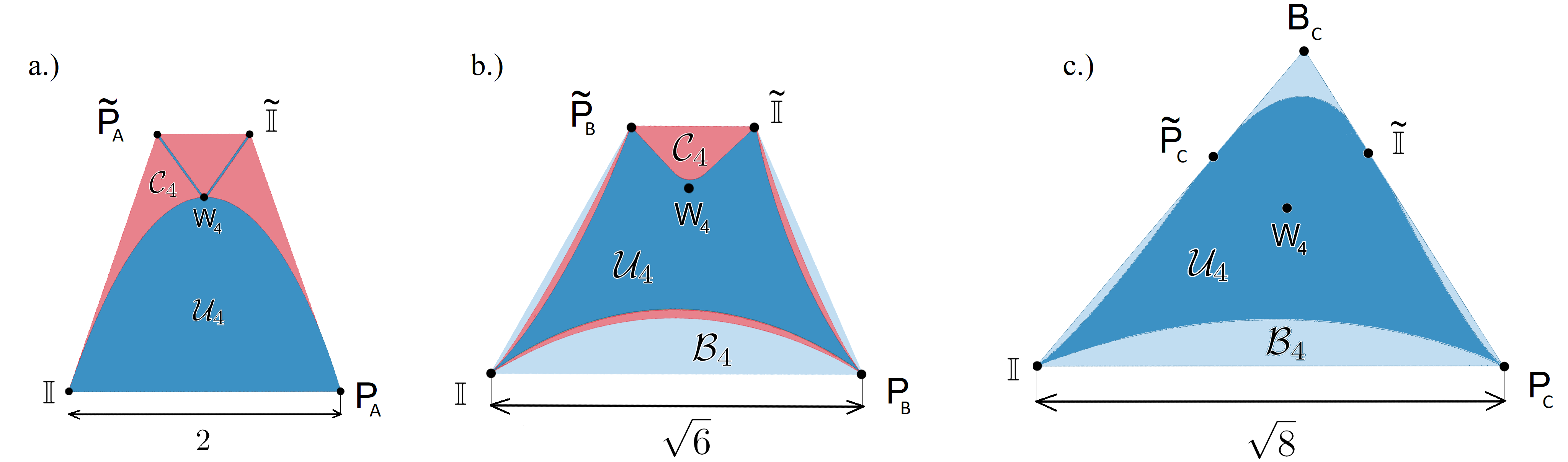
Figure 2: Cross-sections of the Birkhoff polytope $\mathcal{B}_{4}$: the flat matrix $W_{4}$ in the center, determined by selected edges:

1. unistochastic short edge $\mathbb{I}\leftrightarrow P_{A}$ of length $2$

2. not unistochastic middle edge $\mathbb{I}\leftrightarrow P_{B}$ of length $\sqrt{6}$

3. not unistochastic long edge $\mathbb{I}\leftrightarrow P_{C}$ of length $\sqrt{8}$

Darkest gray (in color: dark blue) represents unistochastic set $\mathcal{U}_{4}$, medium gray (red) represents the set $\mathcal{C}_{4}$ of matrices that satisfy the chain conditions, and the lightest gray (light blue) denotes bistochastic matrices, that do not satisfy chain conditions. At the section showed in panel c) the sets $\mathcal{U}_{4}$ and $\mathcal{C}_{4}$ do coincide, while the bistochastic matrix at the edge reads $B_{c}=2W_{4}-\frac{1}{2}P_{c}-\frac{1}{2}\mathbb{I}_{4}$. Note the dark sets $\mathcal{U}_{4}$ in all panels containing both counter-rays are not convex but are star-shaped.

To produce each plot we generated a lattice of around $10^{4}$ bistochastic matrices belonging to a given 2D cross–section and verified if conditions (3.1) are satisfied and whether numerical procedure described in Appendix A returns the corresponding unitary matrix. The Birkhoff polytope $\mathcal{B}_{4}$ possesses an interesting property – in every neighborhood of the flat unistochastic matrix $W_{4}$ localized at its center there are non-unistochastic matrices. Hence there is a direction, in which deviation by an arbitrary small $\epsilon$ leads to a matrix which is not unistochastic [5]. Selecting one of those directions according to [5] we find a cross-section shown in Fig. 3, such that non-unistochastic matrices are located arbitrary close to $W_{4}$:

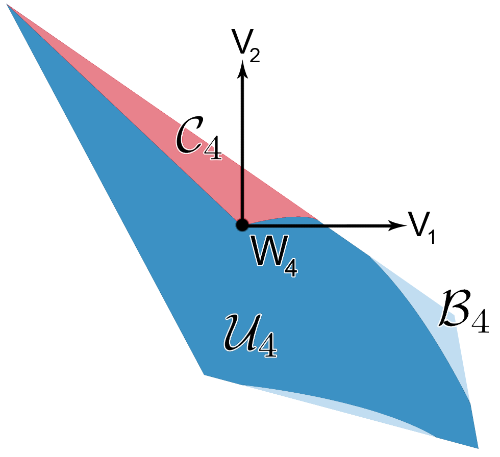
Figure 3: Cross-section of the Birkhoff polytope $\mathcal{B}_{4}$, determined by the directions $V_{1}$ and $V_{2}$ described in [5]. The flat matrix $W_{4}$ in the center of the $\mathcal{B}_{4}$ is also localized at the boundary of the set $\mathcal{U}_{4}$. Colors have the same meaning as in Fig. 2.

Our findings do not contradict the conjecture, that the set ${\mathcal{U}}_{4}$ of unistochastic matrices is star-shaped with respect to $W_{4}$. There exist 2D cross-sections, in which the sets ${\mathcal{U}}_{4}$ and ${\mathcal{C}}_{4}$ coincide, but it is easy to find a cross-section which reveals that the inclusion relation $\mathcal{U}_{4}\subset\mathcal{C}_{4}$ is proper. Compare the discussion of relative volumes of these sets presented in Appendix B.

7 Concluding remarks

A notion of Hadamard matrices robust with respect to a projection onto a subspace formed by any two of the basis vectors is introduced. In the case of a double even dimension, $n=4k$, existence of such matrices follows from existence of skew real Hadamard matrices. Furthermore, existence of symmetric conference matrices of dimension $n=4k+2$ with $k\geq 1$ yields a construction of a robust complex Hadamard matrix of this size. This implies that robust Hadamard matrices exist for all even dimensions $n\leq 20$.

Existence of robust Hadamard matrices of order $n$ allows us to show that all the rays of the Birkhoff polytope ${\mathcal{B}}_{n}$ of bistochastic matrices are unistochastic. Hence for any point $B_{a}$ at the line joining an edge (a permutation matrix) with the flat matrix $W_{n}$ at the center of the polytope, there exists a corresponding unitary matrix $U(a)$ of size $n$ such that $B_{a}=U(a)\circ{\bar{U}(a)}$. Furthermore, if two permutation matrices $P$ and $Q$ are strongly complementary [2] – see Definition 4.3 – the entire triangle $\Delta(P,Q,W_{n})$ is unistochastic.

The family of unitary matrices $U(a)$ of order $n$ obtained with help of robust Hadamard matrices of size $n$, allows us to construct a family of equi-entangled bases in the composed Hilbert space of $n\times n$ system. This family interpolates between the separable basis and the maximally entangled basis. Each interpolating basis consists of $n^{2}$ normalized vectors with the same Schmidt vectors, which determine the entropy of entanglement (5.4). In contrast to the earlier constructions given in [18] and extended in [14] our construction is based on a straight line in the Birkhoff polytope ${\mathcal{B}}_{n}$, so the Schmidt vectors contain only two different entries.

This work contributes to investigations [5] of the set ${\mathcal{U}}_{4}$ of unistochastic matrices of order $n=4$. Making use of the Haagerup algorithm to verify numerically whether a given bistochastic matrix $B\in{\mathcal{B}}_{4}$ is unistochastic – see Appendix A – we provided a first estimation of the relative volume of the set ${\mathcal{U}}_{4}$ of unistochastic matrices and the larger set $\mathcal{C}_{4}$ of these bistochastic matrices, which satisfy all chain conditions (3.1) and (3.2). Furthermore, we studied the geometry of cross-sections of the set ${\mathcal{U}}_{4}$ along planes determined by selected permutation matrices – corners of the Birkhoff polytope ${\mathcal{B}}_{4}$.

Let us conclude the paper with a short list of open questions.

1. Given a Hadamard matrix $H$ of order $n$ is it possible to find an equivalent robust matrix, $H^{R}\sim H$? Due to Lemma 2.7 this question is analogous to the problem concerning existence of skew Hadamard matrices.

2. What are the properties of the set of robust Hadamard matrices in dimension $n$ for which there exists several not equivalent Hadamard matrices $(n=16,\,20,\,\dots)$?

3. Is the convex hull of all mutually strong complementary permutation matrices of a fixed order $n$ and the flat matrix $W_{n}$ unistochastic?

4. Is it possible to obtain necessary and sufficient conditions for unistochasticity applicable for any bistochastic matrix of order $n\geq 5$?

5. For any large dimension $n$, a generic bistochastic matrix is conjectured to meet all chain conditions – see Appendix B. Following question remains open: what is the dependence of fraction of unistochastic matrices $f_{u}$ on dimension $n$ for $n\geq 5$?

Acknowledgements. One of the authors (K.Ż.) had a chance to discuss the unistochasticity problem with the late Uffe Haagerup during the conference in Będlewo in July 2014, where he learned about the way to treat the $n=4$ case presented in the Appendix A. It is a pleasure to thank Ingemar Bengtsson and Irina Dimitru for numerous discussions on equi-entangled bases and for sharing with us their unpublished notes. We are thankful to Dardo Goyeneche and Wojciech Tadej for numerous interactions and also to Robert Craigen and William Orrick for fruitful discussions during the workshop in Budapest in July 2017. Special thanks are due to Mate Matolcsi and Ferenc Szöllősi, for organizing such a successful conference which made these interactions possible. We are deeply obliged to the referee for a long list of constructive comments, valuable hints to the literature and for suggesting us results presented in Appendix D. Financial support by Narodowe Centrum Nauki under the grant number DEC-2015/18/A/ST2/00274 is gratefully acknowledged.

Appendix A. Haagerup procedure for studying unistochasticity of $n=4$ matrices.

In this appendix we present a method due to the late Uffe Haagerup of searching for a unitary matrix corresponding to any unistochastic matrix of order $n=4$. Given a bistochastic matrix $B\in\mathcal{B}_{4}$ we wish to find $U$ such that $B_{ij}=|U_{ij}|^{2}$.

Any matrix of order four can be decomposed into four blocks of order two. Let us then represent in this way the unitary matrix $U$ we are looking for,

$$U=\left(\begin{array}[]{c|c}A&X\\ \hline\cr Y&D\end{array}\right)=\left(\begin{array}[]{llll}\sqrt{B_{11}}&\sqrt{B_{12}}&\sqrt{B_{13}}&\sqrt{B_{14}}\\ \sqrt{B_{21}}&\sqrt{B_{22}}e^{i\phi}&\sqrt{B_{23}}e^{i\alpha_{1}}&\sqrt{B_{24}}e^{i\alpha_{2}}\\ \sqrt{B_{31}}&\sqrt{B_{32}}e^{i\beta_{1}}&\cdot&\cdot\\ \sqrt{B_{41}}&\sqrt{B_{42}}e^{i\beta_{2}}&\cdot&\cdot\end{array}\right)\ ,$$ (7.1)

Note that all the moduli are determined by the bistochastic matrix $B$, so only the phases remain unknown. Unitarity of $U$ implies that

$$UU^{*}=\mathbb{I}\hskip 14.22636pt\Rightarrow\hskip 14.22636pt\left\{\begin{array}[]{l}AA^{*}+XX^{*}=\mathbb{I}\\ \\ AY^{*}+XD^{*}=0\ .\end{array}\right.$$ (7.2)

Due to existence of the Hadamard matrix $H_{4}$ we know that the flat matrix $W_{4}$ is orthostochastic, so we can assume that $B\neq W_{4}$. Permuting rows and columns of $B$ one can rearrange the matrix in such a way that the following relation holds

$$B_{11}+B_{12}+B_{21}+B_{22}<1\ .$$

After this is done the norm of the block $A$ is bounded,

$$||A||^{2}_{\rm HS}<1\hskip 8.53581pt\Rightarrow\hskip 8.53581pt\mbox{eigenvalue}(AA^{*})<1\hskip 8.53581pt\Rightarrow\hskip 8.53581pt\mbox{eigenvalue}(XX^{*})>0\ ,$$

so the neighboring block $X$ is invertible. Hence we can use the matrix $X^{-1}$ to transform the second unitarity condition in (7.2) into an explicit expression for the lower diagonal block $D$,

$$D=-YA^{*}(X^{*})^{-1}\ .$$ (7.3)

The next step is to find the phases in the blocks $X$ and $Y$. To take into account orthogonality between the first two rows of the matrix $U$, it is convenient to introduce four auxiliary variables,

$$l_{1}=\sqrt{B_{11}B_{21}}\ ,\hskip 11.38109ptl_{2}=\sqrt{B_{12}B_{22}}\ ,\hskip 11.38109ptl_{3}=\sqrt{B_{13}B_{23}}\ ,\hskip 11.38109ptl_{4}=\sqrt{B_{14}B_{24}}\ .$$

They allow us to rewrite this orthogonality condition,

$$l_{1}+l_{2}e^{i\phi}+l_{3}e^{i\alpha_{1}}+l_{4}e^{i\alpha_{2}}=0\,$$ (7.4)

which can be treated as an equation for the unknown phases. Orthogonality requires that a chain formed out of four links of lengths $l_{i}$ has to be closed, so the longest link is not longer than the sum of remaining links,

$$l_{i}\leq\frac{1}{2}\sum^{4}_{j=1}l_{j}\quad\textrm{for}\quad i=1,\dots,4.$$ (7.5)

If this condition is not satisfied, the matrix $B$ is clearly not unistochastic. Observe that these conditions can be interpreted as particular cases of the general conditions (3.1) and (3.2).

If inequalities (7.5) are fulfilled there exist two solutions of eq. (7.4) corresponding to a convex and a non-convex polygon,

$$\alpha_{1}=\alpha_{1}(\phi)\ ,\hskip 17.07164pt\alpha_{2}=\alpha_{2}(\phi)\$$

which depend on the phase $\phi$ treated here as a free parameter.

Making use of the orthogonality condition between two first columns of $U$ we arrive at an equation analogous to (7.4), which for a given phase $\phi$ can be solved for unknown phases $\beta_{1}$ and $\beta_{2}$. This determines the blocks $X$ and $Y$ and allows us to obtain the remaining block $D$ of $U$.

The catch is that the explicit formula (7.3) produces a matrix $D$, which needs not to be compatible with the structure imposed by the initial bistochastic matrix $B$. To find the desired unitary matrix $U$ it is sufficient to check that a single element of $D$ has the correct norm. Hence we arrive at the following criterion for unistochasticity for a matrix $B$ of order four:

A bistochastic matrix $B\in\mathcal{B}_{4}$ is unistochastic if there exist a phase $\phi$ entering eq. (7.1), (which determines phases $\alpha_{i}$ and $\beta_{i}$ and thus blocks $X$ and $Y$), such that the block $D$ obtained by eq. (7.3) satisfies the constraint $|D_{11}|^{2}=B_{33}$.

If this is the case the unitary matrix $U$ given by the form (7.1) satisfies the unistochasticity condition, conveniently written by the Hadamard product, $B=U\circ{\bar{U}}$. Note that the above procedure can be easily implemented numerically for any given bistochastic matrix $B\neq W_{4}$ of order four.

Appendix B. Unistochasticity and chain link conditions in small dimensions – numerical results

Random points in a cube. The simplest method to generate a random bistochastic matrix $B$ from the Birkhoff polytope $\mathcal{B}_{n}$ with respect to the uniform measure is to take random numbers, uniformly distributed in $[0,1]$ for each entry of the core – the principal submatrix of order $n-1$, which determines the matrix $B$. If the sum of any row or column of the core is greater than $1$ or the sum of all elements of the core is smaller than $n-2$, then the generated matrix is not bistochastic and will not be considered. If all these conditions are met, we generate a bistochastic matrix by filling the missing row and column with values which will add up all rows and columns to $1$. The entry $B_{nn}$ is equal to the sum of all elements of the core reduced by $n-1$.

To optimize computational procedure of generating the cores, we use row discrimination. Drawing the core row-by-row (rows are independent) allows one to check the sum of the row at every step and stop the procedure if it exceeds unity. This method occurs to work efficiently for dimensions $n\leq 6$, so for higher dimensions one needs to apply other techniques [7, 9].

Sinkhorn algorithm To generate a bistochastic matrix for $n\geq 7$ we also used a method described in [7], analogous to the Sinkhorn algorithm [27], which normalizes rows and columns of a given square matrix in a following sequence:

1. input a random stochastic matrix of dimension $n$ with positive elements,

2. normalize every row by dividing it by the sum of its elements,

3. normalize every column of the matrix by dividing it by the sum of its elements,

4. go to point 2., unless the matrix is bistochastic up to a certain accuracy with respect to the chosen norm.

In practice we stopped the procedure if all the sums of rows and vectors are close to unity up to the sixth decimal place $(0.9999999\leq\varSigma rows,\varSigma columns\leq 1.0000001)$. This procedure occurs to be much faster than taking points at random from the core for dimensions $n>6$.

Dirichlet distribution. It is natural to study the measure induced in $\mathcal{B}_{n}$ by the Sinkhorn algorithm applied to random stochastic matrices with entries described by the Dirichlet distribution [20], $P_{s}(x_{1},\dots,x_{n})\propto\prod^{n}_{i=1}x^{1-s}_{i}$, with the constraint $\sum_{i}x_{i}=1$. For $s=1$ this distribution coincides with the uniform distribution in the probability simplex. For a certain value of the parameter $s_{*}=\frac{1}{2n^{2}}(n^{2}-2+\sqrt{n^{4}-4})$ the measure induced in the set of bistochastic matrices becomes uniform [7] in the limit of large $n$.

To generate a sequence of $n$ numbers distributed according to Dirichlet distribution with a chosen parameter $s$ we used the following sequence:

1. generate $n$ independent random numbers from the gamma distribution of rate $1$ and shape $s$. Explicitly, every element of $(x_{1},x_{2},\ldots,x_{n})$, is drawn with probability density $\frac{1}{\Gamma(s)}x^{s-1}e^{-x}$.

2. normalize every element by dividing it by the sum of all elements, $x_{i}\to x^{\prime}_{i}=\frac{1}{\underset{i}{\sum x_{i}}}x_{i}$.

Applying the above procedure $n$ times we obtain random stochastic matrix of $n$ independent rows each distributed according to Dirichlet distribution. Making use of the Sinkhorn algorithm we to obtain an ensemble of bistochastic matrices which is uniformly distributed at the center of the Birkhoff polytope.

Numerical computations show that the first method (generating random points in a cube) is reliable for $n\leq 6$, while for $n>6$ the Sinkhorn method, used with the Dirichlet parameter $s_{*}$, becomes more efficient. A numerical estimation of the relative volume of the set of unistochastic matrices is shown in Fig. 4. Note that the relative volume of the set $\mathcal{C}_{n}$ of matrices satisfying the chain conditions approaches unity.

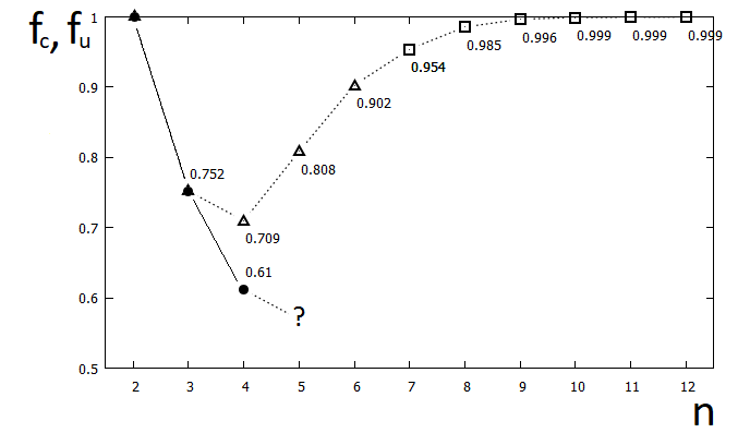
Figure 4: Fraction $f_{u}$ of random bistochastic matrices, generated with respect to the flat measure, satisfying unistochasticity conditions (black circle – $\bullet$) computed for dimensions $n<5$. Empty symbols (white triangle – ${\bigtriangleup}$ and white square – $\square$) denote the fraction $f_{c}$ of bistochastic matrices, which fulfill all chain conditions (3.1-3.2). Dotted line is plotted to guide the eye.

Appendix C. No robust Hadamard matrices of order $3$ and $5$

To analyze whether a complex Hadamard matrix $H^{\prime}$ of order $n$ satisfies the equivalence relation (2.1) with respect to a given Hadamard matrix $H$ one can use the set of invariants of Haagerup [15],

$$\Lambda_{ij,kl}:=H_{ij}{\bar{H}_{kj}}H_{kl}{\bar{H}_{il}},$$ (7.6)

where no summation over repeated indices is assumed and $i,j,k,l=1,\dots,n$. The complex numbers $\Lambda_{ij,kl}$, depending on the cumulative difference of phases, are invariant with respect to multiplication of $H$ by diagonal unitary matrices. Even though these $n^{4}$ complex numbers may be altered by permutations of rows and columns, the entire set $\Lambda(H)=\{\Lambda_{ij,kl}\}_{i,j,k,l=1}^{n}$ remains invariant with respect to the equivalence relation (2.1).

In the case of the Hadamard matrix $H_{2}$ the set of invariants $\Lambda(H_{2})$ contains the number $-1$ corresponding to the phase $\pi$. Hence the set $\Lambda(H^{R})$ for a robust Hadamard matrix $H^{R}$ of order $n$ has to contain at least $n(n-1)/2$ these entries.

Consider now a Fourier matrix $F_{n}$ with $n>1$ and entries

$$\mathcal{(}F_{n})_{jk}={e}^{i(j-1)(k-1)2\pi/n},$$ (7.7)

with $j,k=1,\dots,n$, which is a complex Hadamard matrix. If the dimension $n$ is odd the set of Haagerup invariants $\Lambda(F_{n})$ does not include the number $-1$ as adding multiples of the basic phase $2\pi/n$ one cannot obtain $\pi$. This implies directly that for any odd number $n>1$ the Fourier matrix $F_{n}$ and any equivalent complex Hadamard matrix is not robust. Since for $n=3$ and $n=5$ all complex Hadamard matrices are equivalent to the Fourier matrix [15], we arrive at the desired statement.

Proposition. There are no robust Hadamard matrices of dimension $n=3$ and $n=5$.

Alternatively, to show that there are no robust Hadamard matrices of order $3$ one can use the result of Cohn [8], who establishes that "there is no room for a sub-Hadamard matrix of size $m$ within a Hadamard matrix of size $n$, where $m>n/2$."

Appendix D. On existence of robust Hadamard matrices

In this Appendix we provide results concerning existence of robust Hadamard matrices which were suggested by the referee and go beyond the statements formulated in Appendix C.

Let $C$ be a complex conference matrix of order $n$, that is $C_{jj}=0$, $|C_{jk}|=1$ and $CC^{*}=(n-1)\mathbb{I}$.

Lemma 7.1.

If $R$ is a robust Hadamard matrix of order $n\geq 2$, then $R$ is equivalent in the sense of eq. (2.4) to a matrix $H=C+i\mathbb{I}$, where $C$ is a self-adjoint complex conference matrix.

Proof.

The relation between $R$ and $H$ is explicitly:

$$H=iRD^{*}$$

where $D$ is the diagonal matrix containing diagonal entries of $R$ and $i$ is imaginary unit. All of the diagonal elements of $H$ are equal to $i$. Because D is a unitary matrix, then $R\sim H$ and thus $H$ is a robust Hadamard matrix. This implies that any principal submatrix of H of order two,

$$M_{2}=\begin{pmatrix}i&h_{jk}\\ h_{kj}&i\\ \end{pmatrix}$$

has to satisfy $|{\rm det}(M_{2})|=2$. Because $|h_{jk}|=1$ for any $j,k$, then $h_{jk}=h_{kj}^{*}$. It implies that the matrix consisting of off-diagonal elements of $H$, namely $C=H-i\mathbb{I}$ is self-adjoint $(C=C^{*})$ and $|C_{jk}|=1$ for $j\neq k$. Self-adjointness of $C$, it implies that $H-H^{*}=2i\mathbb{I}$. Finally we can obtain:

$$CC^{*}=(H-i\mathbb{I})(H^{*}+i\mathbb{I})=HH^{*}+i(H-H^{*})+\mathbb{I}=n\mathbb{I}-2\mathbb{I}+\mathbb{I}=(n-1)\mathbb{I}$$

which completes the proof. ∎

Above result shows that robust complex Hadamard matrices are essentially a family of matrices equivalent to self-adjoint complex conference matrices with the diagonal elements filled with imaginary unit $i$.

Lemma 7.2.

If a robust Hadamard matrix $H$ of order $n$ exists, then $n$ is even.

Proof.

Applying Lemma 7.1 we can restrict ourselves to the case $H=C+i\mathbb{I}$. Since $C=C^{*}$ and $C$ is unitary up to scalar, then its spectrum is real and the eigenvalues are equal to $\pm\sqrt{n-1}$. Note also that $C$ is traceless. Therefore, for $n\geq 2$, the number of positive and negative eigenvalues must be equal. It follows that the number of eigenvalues, which is equal to $n$, must be even. ∎

References

- [1] G. Auberson, A. Martin and G. Mennessier, On the reconstruction of a unitary matrix from its moduli, Commun. Math. Phys. 140, 417-437 (1991).
- [2] Y.H. Au-Yeng and C.M. Cheng, Permutation matrices whose convex combinations are orthostochastic, Lin. Alg. Appl. 150, 243-253 (1991).
- [3] Y.H. Au-Yeng and Y.T. Poon, Orthostochastic matrices and the convexity of generalized numerical ranges, Lin. Alg. Appl. 27, 69-79 (1979).
- [4] I. Bengtsson and I. Dumitru, Isoentangled orbits and isoentangled bases, working notes, Stockholm, 2016.
- [5] I. Bengtsson, A. Ericsson, M. Kuś, W. Tadej, K. Życzkowski, Birkhoff’s polytope and unistochastic matrices, and , Commun. Math. Phys. 259, 307-324 (2005).
- [6] G. Birkhoff, Tres observaciones sobre el algebra lineal, Univ. Nac. Tucumán Rev. A5, 147 (1946).
- [7] V. Cappellini H.-J. Sommers, W. Bruzda and K. Życzkowski, Random bistochastic matrices, J. Phys. A 42, 365209 (2009).
- [8] J. H. E. Cohn, Hadamard matrices and some generalisations, Amer. Math. Monthly 72, 515-518 (1965).
- [9] B. Collins, T. Kousha, R. Kulik, T. Szarek, and K. Życzkowski, The Accessibility of Convex Bodies and Derandomization of the Hit and Run Algorithm, J. Convex Anal. 24, 903-916 (2017).
- [10] R. Craigen, Equivalence classes of inverse orthogonal and unit Hadamard matrices, Bull. Austr. Math. Soc. 44, 109-115 (1991).
- [11] P. Diţǎ, Separation of unistochastic matrices from the double stochastic ones. Recovery of a unitary matrix from experimental data, J. Math. Phys. 47, 083510 (2006).
- [12] C. Dunkl and K. Życzkowski, Volume of the set of unistochastic matrices of order 3 and the mean Jarlskog invariant, J. Math. Phys. 50, 123521 (2009).
- [13] D. Goyeneche and O. Turek, Equiangular tight frames and unistochastic matrices, J. Phys. A 50, 245304 (2017).
- [14] V. Gheorghiu and S. Y. Loo, Construction of equientangled bases in arbitrary dimensions via quadratic Gauss sums and graph states, Phys. Rev. A 81, 062341 (2010).
- [15] U. Haagerup, Orthogonal maximal abelian -subalgebras of the matrices and cyclic –rots, Operator Algebras and Quantum Field Theory (Rome), (Cambridge, MA: International Press) pp 296-322 (1996).
- [16] K.J. Horadam, Hadamard Matrices and Their Applications, Princeton University Press, Princeton 2007.
- [17] C. Jarlskog and R. Stora, Phys. Lett. B 208, 268 (1988).
- [18] V. Karimipour and L. Memarzadeh, Equientangled bases in arbitrary dimensions, Phys. Rev. A 73, 012329 (2006).
- [19] B.R. Karlsson, -reducible complex Hadamard matrices of order , Lin. Alg. Appl. 434, 239-246 (2011).
- [20] J. F. C. Kingman, Random discrete distributions, J. Roy. Statist. Soc. B 37, 1-22 (1975).
- [21] C. Koukouvinos and S. Stylianou, On skew-Hadamard matrices, Discrete Mathematics 308, 2723-2731 (2008).
- [22] J.H. van Lint and J.J. Seidel, Equilateral point sets in elliptic geometry, Indag. Math. 28, 335-348 (1966).
- [23] H. Nakazato, Set of orthostochastic matrices, Nihonkai Math. J. 7, 83-100 (1996).
- [24] W. P. Orrick, Switching operations for Hadamard matrices. SIAM J. Discrete Math. 22, 31-50 (2008).
- [25] P. Pakoński, Ph.D. thesis, Jagiellonian University, 2002.
- [26] P. Pakoński, K. Życzkowski, M. Kuś, Classical 1D maps, quantum graphs and ensembles of unitary matrices, J. Phys. A 34, 9303-9317 (2001).
- [27] R. Sinkhorn, A relationship between arbitrary positive matrices and doubly stochastic matrices, Ann. Math. Statist. 35, 876–879 (1964).
- [28] F. Szöllősi, Construction, classification and parametrization of complex Hadamard matrices, preprint arXiv:1110.5590, (2011).
- [29] W. Tadej, K. Życzkowski, A concise guide to complex Hadamard matrices, Open Syst. Inf. Dyn. 13, 133-177 (2006).
- [30] R. F. Werner, All teleportation and dense coding schemes, J. Phys. A 34, 7081 (2001).
- [31] K. Życzkowski, M. Kuś, W. Słomczyński and H.-J. Sommers, Random unistochastic matrices, J. Phys. A 36, 3425-3450 (2003).