Alternative parameterizations of Metric Dimension

Abstract

A set of vertices $W$ in a graph $G$ is called resolving if for any two distinct $x,y\in V(G)$, there is $v\in W$ such that $\operatorname{d}_{G}(v,x)\neq\operatorname{d}_{G}(v,y)$, where $\operatorname{d}_{G}(u,v)$ denotes the length of a shortest path between $u$ and $v$ in the graph $G$. The metric dimension $\textrm{md}(G)$ of $G$ is the minimum cardinality of a resolving set. The Metric Dimension problem, deciding whether $\textrm{md}(G)\leqslant k$, is NP-complete even for interval graphs (Foucaud , 2017). We study Metric Dimension (for arbitrary graphs) from the lens of parameterized complexity. The problem parameterized by $k$ was proved to be $\W[2]$-hard by Hartung and Nichterlein (2013) and we study the dual parameterization, i.e., the problem of whether $\textrm{md}(G)\leqslant n-k,$ where $n$ is the order of $G$. We prove that the dual parameterization admits (a) a kernel with at most $3k^{4}$ vertices and (b) an algorithm of runtime $O^{*}(4^{k+o(k)}).$ Hartung and Nichterlein (2013) also observed that Metric Dimension is fixed-parameter tractable when parameterized by the vertex cover number $vc(G)$ of the input graph. We complement this observation by showing that it does not admit a polynomial kernel even when parameterized by $vc(G)+k$. Our reduction also gives evidence for non-existence of polynomial Turing kernels.

1 Introduction

A set of vertices $W$ of a graph $G$ is a resolving set for $G$ if for any two distinct $x,y\in V(G)$, there is $v\in W$ such that $\operatorname{d}_{G}(v,x)\neq\operatorname{d}_{G}(v,y)$, where $\operatorname{d}_{G}(u,v)$ denotes the length of a shortest path between $u$ and $v$ in the graph $G$. The metric dimension $\textrm{md}(G)$ of $G$ is the minimum cardinality of a resolving set for $G$. The metric dimension of graphs was introduced independently by Slater [25] and Harary and Melter [16]. Metric Dimension as a computational problem was first mentioned in the literature by Garey and Johnson [14] and its decision version is defined as follows.

Garey and Johnson [14] proved this problem to be NP-complete in general. Their proof was never published, a reduction from 3SAT was provided by Khuller  [21]. Diaz  [6] showed that the problem is NP-complete even when restricted to planar graphs of bounded degree but that it is solvable in polynomial time on the class of outer-planar graphs.

Prior to this, not much was known about the computational complexity of this problem except that it is polynomial-time solvable on trees (see [25, 21]), although there are several results proving combinatorial bounds on the metric dimension of various graph classes [3]. Subsequently, Epstein et al. [10] showed that this problem is NP-complete on split graphs, bipartite and co-bipartite graphs. They also showed that the weighted version of Metric Dimension can be solved in polynomial time on paths, trees, cycles, co-graphs and trees augmented with $k$ edges for a fixed $k$. Hoffmann and Wanke [19] extended the tractability results to a subclass of unit disk graphs, while Foucaud  [12] showed that this problem is NP-complete on interval graphs.

The parameterized complexity of Metric Dimension under the standard parameterization—the metric dimension of the input graph—was open until 2012, when Hartung and Nichterlein [17] proved that it is $\W[2]$-hard. Foucaud  [12] showed the problem becomes fixed-parameter tractable when restricted to interval graphs. The parameterized complexity of Metric Dimension on graphs of bounded treewidth is currently unresolved (the question of whether it is polynomial-time solvable on graphs of treewidth 2 is still open), however, Belmonte  [2] proved that it is $\FPT$ when parameterized by the treelength plus the solution size. In a different line of work, Eppstein [9] showed that Metric Dimension is $\FPT$ when parameterized by the max-leaf number of the input graph alone.

In this paper we initiate the study of the parametric dual of Metric Dimension. To avoid confusion, we will use $k$ to denote the (standard) parameter and phrase the parameterized dual as follows:

We call a set $T$ of vertices of $G$ a co-resolving set if $V(G)\setminus T$ is a resolving set of $G$. Clearly, an instance of Saving Landmarks is positive if and only if there is a co-resolving set $T$ of size at least $k$.

This choice of parameterization is informed by previous studies of the parametric dual (see e.g. [1, 4, 15, 24]): problems that are hard with respect to the standard parameter often admit an $\FPT$-algorithms or even polynomial kernels under the dual parameter. A classic example is the Independent Set problem which is $\W[1]$-hard while its dual, the Vertex Cover problem is among the earliest problems shown to be in $\FPT$ and even admits a linear vertex kernel.

We add yet another entry to the list of hard problems with tractable duals by showing that Saving Landmarks admits a polynomial kernel and a single-exponential $\FPT$ algorithm. Concretely, we prove the following two results.

Theorem 1.

Saving Landmarks admits a kernel with at most $8k^{4}$ vertices.

Theorem 2.

Saving Landmarks can be solved in time $O^{*}(4^{k+o(k)})$.

We also study the Metric Dimension problem from the kernelization perspective when parameterized by the vertex cover number of the input graph. As Hartung and Nichterlein observed [17], parameterization of Metric Dimension by the vertex cover number of the input graph (denoted Metric Dimension[VC]) can be easily seen to be in $\FPT$. It is therefore natural to ask whether this structural parameterization allows a polynomial kernel in general graphs, a question we answer in the negative. In fact, we show that not only does the problem not admit a polynomial kernel with the vertex cover as the parameter, even adding the size of the solution (the metric dimension of the graph) to the parameter is unlikely to be helpful in this regard. Specifically, we prove the following result.

Theorem 3.

Metric Dimension[$\text{VC}+k$] does not admit a polynomial kernel unless the polynomial hierarchy collapses to its third level.

The reduction used in the proof of Theorem 3 also gives evidence for non-existence of polynomial Turing kernels, generalizations of (ordinary) kernels, informally introduced in the end of Section 4.

2 Preliminaries

For a graph $G$ we denote by $\operatorname{d}_{G}$ the standard distance-metric where $\operatorname{d}_{G}(u,v)$ is the length of a shortest path between vertices $u,v\in V(G)$. We denote by $N_{G}(v)$ and $N_{G}[v]$ the open and closed neighbourhood of a vertex. We omit the subscript $G$ if clear from the context in all these notations. As customary, the number of vertices of a graph $G$ under consideration will be denoted by $n.$

Two vertices $u,v$ are true twins if $N_{G}[u]=N_{G}[v]$ (implying that $uv\in G$) and they are false twins if $N_{G}(u)=N_{G}(v)$. A twin class is a maximal vertex set in $G$ in which all vertices are pairwise true twins or in which all vertices are pairwise false twins.

A vertex set $S\subseteq V(G)$ resolves a set $T\subseteq V(G)$ if for every pair of distinct vertices $u,v\in T$ there exists at least one vertex $w\in S$ such that $\operatorname{d}_{G}(u,w)\neq\operatorname{d}_{G}(v,w)$. We will also say that a pair $u,v$ is resolved by $S$ if the above holds and further that sets $A,B$ are distinguished by $S$ if every pair $u\in A$, $v\in B$ is resolved by $S$. A vertex subset $S\subseteq V(G)$ is a resolving set of $G$ if $S$ resolves $V(G)$. We call the members of such a set $S$ landmarks.

Parameterized complexity is a two dimensional framework for studying the computational complexity of a problem. One dimension is the input size $n$ and the other is a parameter $k$. A problem is said to be fixed parameter tractable ($\FPT$) or in the class $\FPT$, if it can be solved in time $f(k)\cdot n^{O(1)}$ for some computable function $f$. We refer to the books of Cygan  [5] and Downey and Fellows [8] for detailed introductions to parameterized complexity.

Kernelization offers a mathematically rigorous way of analysing and comparing preprocessing algorithms for $\NP$-hard problems in general and for parameterized problems in particular. A kernel of size $g(k)$ for a parameterized problem is a polynomial time algorithm that takes as input an instance $(I,k)$ of the problem (where $k$ is the parameter) and outputs another instance $(I^{\prime},k^{\prime})$ of the same problem such that $(I,k)$ is a yes- instance of the problem if and only if $(I^{\prime},k^{\prime})$ is a yes-instance of the problem and $|I^{\prime}|+k^{\prime}\leqslant g(k)$. The notion of “effective” preprocessing is captured by requiring the function $g$ to be polynomially bounded, in which case the kernel is called a polynomial kernel. The reader is referred to Cygan  [5], Downey and Fellows [8], Fomin [11] and the surveys [22, 23] for a comprehensive introduction to the topic of kernelization.

Definition 4 (Pruned graph).

For a graph $G$ we define the pruned graph $\widetilde{G}$ as the graph obtained (up to isomorphism) from $G$ by iteratively removing vertices from twin-classes of size three or larger. We say that a graph is pruned if $G=\widetilde{G}$.

The following observation simply follows from the fact that among a twin class $U$ in $G$, all but one vertex of $U$ must be contained in any resolving set.

Observation 5.

A graph $G$ has a resolving set of size $k$ if and only if the pruned graph $\tilde{G}$ has a resolving set of size $k-(|V(G)|-|V(\tilde{G})|)$.

Consequently, we call an instance $(G,k)$ of Metric Dimension or Saving Landmarks reduced if $G$ is pruned.

3 Standard parameterization for Saving Landmarks

We present two positive results in this section, namely, that Saving Landmarks admits a polynomial kernel and a single-exponential $\FPT$ algorithm.

We begin by describing the kernel. Assume in the following that the input instance $(G,k)$ is pruned as per Observation 5. This will be the only reduction rule. In the following we will prove that the size of the instance is either bounded polynomially in $k$ or it will be a trivial yes-instance. Let us collect some basic observations first.

Lemma 6.

If $G$ contains either an independent set or a clique with $2k$ vertices, then $(G,k)$ is a yes-instance.

Proof.

Let $X$ be a set of size $2k$ such that $G[X]$ is either a clique or an independent set. Since $G$ is pruned there are at least $|X|/2\geqslant k$ distinct twin-classes in $X$, which must be distinguished by their neighbourhoods outside of $X$. Hence selecting one vertex from each twin-class in $X$ gives a co-resolving set of size at least $k$, and $(G,k)$ is a yes-instance.

Let us define the function $\tau(u,v):=|N(u)\mathop{\vartriangle}N(v)|$. Note that if $\tau(u,v)\geqslant k+1$, then $u$ and $v$ are distinguished from each other by any set of $n-k$ landmarks, simply by virtue of having a necessarily different set of landmarks as neighbours. Let us therefore construct an auxiliary graph $H$ on $V(G)$ where

$$uv\in E(H)\iff\tau(u,v)\leqslant k.$$

Observe that if $H$ contains an independent set $X$ of size $k$ then $(G,k)$ is a yes-instance: the set $V(G)\setminus X$ has size $n-k$ and as such will still resolve all of $X$. This indicates that $H$ must be rather dense, however, we can also argue that it cannot have arbitrarily high degree:

Lemma 7.

Let $v\in V(H)$ have degree at least $8k^{3}$ in $H$. Then $(G,k)$ is a yes-instance.

Proof.

Let $S:=N_{H}[v]$. Note that for every pair $u,u^{\prime}\in S$ it holds that

$$\tau(u,u^{\prime})\leqslant\tau(u,v)+\tau(u^{\prime},v)\leqslant 2k.$$

Now turn our attention to $G$. First consider the case in which every vertex in $G[S]$ has degree less than $4k^{2}$. Then greedily packing closed neighbourhoods gives an independent set in $G$ of size at least $2k$, and by Lemma 6, $(G,k)$ is a yes-instance.

Thus consider the alternative that $G[S]$ contains a vertex $u_{1}$ of degree at least $4k^{2}$. Define $S_{1}:=N_{G[S]}(u_{1})$ and pick any vertex $u_{2}\in S_{1}$. Note that since $\tau(u_{1},u_{2})\leqslant 2k$ it follows that

$$|N_{G[S]}(u_{1})\mathop{\vartriangle}N_{G[S]}(u_{2})|\leqslant|N_{G}(u_{1})\mathop{\vartriangle}N_{G}(u_{2})|\leqslant 2k.$$

Consequently, $u_{1}$ and $u_{2}$ share at least $|S_{1}|-2k-1\geqslant 4k^{2}-2k-1$ neighbours in $G[S]$ (removing one extra since $u_{2}\in S_{1}$). We can repeat this procedure to construct a sequence of distinct vertices $u_{1},u_{2},\ldots,u_{r}$ and subsets $S_{1}\supseteq S_{2}\supseteq\ldots\supseteq S_{r}$ where $S_{i}:=\bigcap_{j\leqslant i}N_{G[S]}(u_{j})$ and $u_{i}\in S_{i-1}$ is chosen arbitrarily. The sequence terminates with $S_{r}=\emptyset$, giving a clique in $G$ of size $r$. Since $|S_{i}|\geqslant|S_{i-1}|-2k-1$ for every $i\in[r]$, we get $|S_{2k-1}|\geqslant|S_{1}|-(2k-2)(2k+1)>0$ since $|S_{1}|\geqslant 4k^{2}$. Thus $r\geqslant 2k$ and $u_{1}$, …, $u_{r}$ induces a clique of size at least $2k$ in $G$, and again by Lemma 6 we conclude that $(G,k)$ is a yes-instance.

With these pieces in place, we can prove the first result of this section.

See 1

Proof.

By Lemma 7 we either have that $(G,k)$ is a yes-instance or that the auxiliary graph $H$ has a maximum degree less than $8k^{3}$. Assuming the latter, if $|V(G)|=|V(H)|\geqslant 8k^{4}$ then $H$ contains an independent set of size at least $k$ and, as observed above, $(G,k)$ is a yes-instance.

The kernel for Saving Landmarks is therefore the following procedure: for a given instance $(G^{\prime},k^{\prime})$, compute the reduced instance $(G,k)$. If $G$ contains more than $8k^{4}$ vertices, return a trivial yes-instance. Otherwise, return $(G,k)$.

Let us now move on to the second result, the single-exponential $\FPT$ algorithm. To better describe the algorithm, let us introduce a definition. For a set $X\subseteq V(G)$, we say that two vertices $u$ and $v$ are $X$-equidistant if $\operatorname{d}(u,w)=\operatorname{d}(v,w)$ for every $w\in X$, i.e., if $X$ fails to resolve $u$ and $v$. Note that this induces an equivalence relation over $V(G)$.

The main ingredient will be fact that a solution to Saving Landmarks is witnessed already by a small resolving set.

Lemma 8.

Let $T$ be a co-resolving set of a graph $G$. Then there exists a set $S\subseteq V(G)\setminus T$ of size at most $|T|$ that resolves $T$.

Proof.

We construct $S$ iteratively as follows. Begin with $S=\emptyset$ and pick a pair $u,v$ of $S$-equidistant vertices in $T$. Since $V(G)\setminus T$ resolves $T$, there exists a vertex $w\in V(G)\setminus T$ that distinguishes $u$ and $v$. Add $w$ to $S$ and partition $T$ into equivalence classes of $S$-equidistant vertices. Pick a new pair of $S$-equidistant vertices from one of the classes and repeat. Observe that the number of equivalence classes increase with every addition to $S$, hence after at most $|T|$ steps the set $S$ resolves every pair in $T$.

We are now ready to complete the proof of Theorem 2.

See 2

Proof.

We may assume that $n\geqslant 2k$. Let us first show the following claim: there exists a co-resolving set $T$ of $G$ of size at least $k$ if and only if there is a partition $V(G)=R\cup B$ of $V(G)$ such that $R$ contains at least $k$ equivalence classes of $B$-equidistant vertices. Suppose that there exists a co-resolving set $T$ of $G$ of size at least $k$. Then by Lemma 8, there is a set $S\subseteq V(G)\setminus T$ of size at most $|T|$ that resolves $T$. Let $T\subseteq R$ and $S\subseteq B$ for a partition $V(G)=R\cup B$. Then $B$ resolves $T$ and hence $R$ has at least $|T|\geqslant k$ equivalence classes of $B$-equidistant vertices. Suppose now that there is a partition $R\cup B$ of $V(G)$ such that $R$ has at least $k$ equivalence classes of $B$-equidistant vertices. Choose a vertex from each equivalence class to form a set $T$. Then $T$ is a co-resolving set of $G$.

The above claim leads to the following randomized algorithm. Choose a natural number $N$ defined later on. Repeat $N$ times the following: uniformly at random partition the vertices of $G$ into $B$ and $R$, and derive equivalence classes of $B$-equidistant vertices in $R$. If the number of classes is at least $k$, then conclude that $(G,k)$ is a yes-instance and stop. If after all repetitions we do not conclude that $(G,k)$ is a yes-instance, then we conclude that $(G,k)$ is a no-instance.

Let us argue about the success probability of the randomized algorithm and how to choose $N$. The probability that for a random partition the vertices of $G$ as $V(G)=R\cup B$, $R$ has at least $k$ equivalence classes of $B$-equidistant vertices is at least the probability that $T\subseteq R$ and $S\subseteq B$, where sets $T,S$ are as in Lemma 8, which is $2^{-|T|-|S|}\geqslant 4^{-k}.$ Thus, $N=4^{k}$ is enough to achieve a constant success probability [5].

Observe that every loop in the randomized algorithm can be executed in polynomial time. Thus, the running time of the randomized algorithm is $O^{*}(4^{k})$. The randomized algorithm can be derandomized using the standard $(n,k)$-universal set technique [5], which brings an additional $o(k)$ to the exponent of the running time.

4 Structural parameterizations for Metric Dimension

As Hartung and Nichterlein observed [17], Metric Dimension[VC] is trivially $\FPT$ by virtue of Observation 5: After reducing the size of each twin class to at most two, any instance with a vertex cover $X$ of size $t$ will have at most $t+2^{t+1}$ vertices. In sparse graph classes, the twin reduction even results in a polynomial-size kernel: in classes of bounded expansion (planar graphs or graphs excluding a topological minor), the number of twin classes in $V(G)\setminus X$ is bounded linearly in $t$ and in nowhere dense classes by $t^{1+o(1)}$ (Lemma 4.3 and Corollary 4.4 in [13]). Furthermore, if the input graphs stem from a $d$-degenerate class, the number of twin-classes and thus the number of vertices in the kernel is bounded by $O(t^{d+1})$; a fact that follows easily from the observation that in such a class at most $dt$ vertices in the independent set can have degree more than $d$.

It is therefore natural to ask whether this structural parameterization allows a polynomial kernel in general graphs, a question we answer in the negative. We will use in the following that Hitting Set parameterized by the size of the universe plus the solution size does not admit a polynomial kernel unless the polynomial hierarchy collapses to the third level [7]

See 3

Proof.

We provide a polynomial parameter transformation from Hitting Set[$|U|+\ell$], i.e. parameterized by the size of the universe and the solution size, to Metric Dimension[$\text{VC}+k$]. Let $(U,\mathcal{F},\ell)$ be a Hitting Set instance with $n=|U|$ and $m=|\mathcal{F}|$. We construct a graph $G$ as follows (Figure 1):

1. Begin with the usual bipartite representation of $U,\mathcal{F}$, i.e., create a bipartite graph $G=(U\cup\mathcal{F},E)$ where for vertices $u\in U$ and $R\in\mathcal{F}$ we have $uR\in E$ if and only if $u\in R$;

2. add $t_{n}:=2\lceil\log_{2}n\rceil$ vertices $I_{U}$ to the graph and edges between $U,I_{U}$ so that every vertex in $U$ has a unique neighbourhood in $I_{U}$ of size $t_{n}/2$;

3. add $t_{m}:=2\lceil\log_{2}m\rceil$ vertices $I_{\mathcal{F}}$ to the graph and edges between ${\mathcal{F}}$ and $I_{\mathcal{F}}$ such that every vertex in ${\mathcal{F}}$ has a unique neighbourhood in $I_{\mathcal{F}}$ of size $t_{m}/2$;

4. add three vertices $a_{U},a,a_{\mathcal{F}}$ where $N(a_{U})=U$, $N(a)=U\cup\mathcal{F}$, and $N(a_{\mathcal{F}})=\mathcal{F}$;

5. create true twin copies $I^{\prime}_{U},I^{\prime}_{\mathcal{F}},a^{\prime}_{U},a^{\prime},a^{\prime}_{\mathcal{F}}$ of $I_{U},I_{\mathcal{F}},a_{U},a,a_{\mathcal{F}}$, and finally

6. create false twin copies $\mathcal{F}^{\prime}$ of $\mathcal{F}$ but remove all edges from $\mathcal{F}^{\prime}$ to $U$ afterwards. For simplicity, we will label the copy of any vertex $R\in\mathcal{F}$ by $R^{\prime}\in\mathcal{F}^{\prime}$.

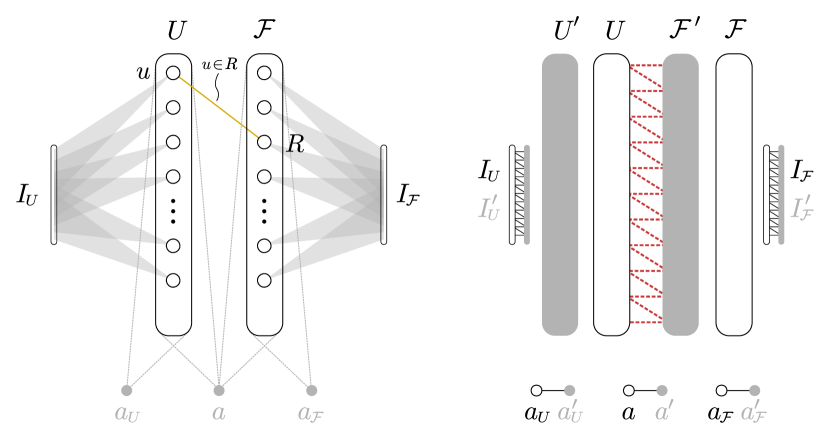
Figure 1: A schematic of the reduction from a Hitting Set[$|U|+\ell$] instance $(U,\mathcal{F})$ to a Metric Dimension[$\text{VC}+k$] instance. The left drawing shows the basic construction, the right drawing the addition of false and true twins (an edge between a white set and its grey counterpart indicates that they are true twins, the absence of an edge that they are false twins). Note that the construction removes edges between the set $U$ and $\mathcal{F}^{\prime}$.

In summary, the sets $I_{U},I^{\prime}_{U}$ connect to $U$ only, the sets $I_{\mathcal{F}},I^{\prime}_{\mathcal{F}}$ to $\mathcal{F}$ and $\mathcal{F}^{\prime}$, the edges between $U,\mathcal{F}$ encode the hitting set instance and the pairs $\{a_{U},a^{\prime}_{U}\}$, $\{a,a^{\prime}\}$, and $\{a_{\mathcal{F}},a^{\prime}_{\mathcal{F}}\}$ are apices for the sets $U$, $U\cup\mathcal{F}\cup\mathcal{F}^{\prime}$ and $\mathcal{F}\cup\mathcal{F}^{\prime}$, respectively. Our construction concludes with $(G,X,k)$ as the Metric Dimension[$\text{VC}+k$] instance with the vertex cover $X:=V(G)\setminus(\mathcal{F}\cup\mathcal{F}^{\prime})$ and solution size $k:=\ell+t_{U}+t_{\mathcal{F}}+3$.

Let us first show that if $(U,\mathcal{F},\ell)$ is a yes-instance then so is $(G,X,k)$. Suppose that $H\subseteq U$ is a hitting set for $\mathcal{F}$ of size $\ell$. We construct a landmark set $S$ for $G$ by setting $S=H\cup I_{U}\cup I_{\mathcal{F}}\cup\{a_{U},a,a_{\mathcal{F}}\}$; let us now argue that is indeed a resolving set. First, note that the selected apices $a_{U}$, $a$, and $a_{\mathcal{F}}$ make sure that $U$ is distinguished from $V(G)\setminus U$ and $\mathcal{F}\cup\mathcal{F}^{\prime}$ from $V(G)\setminus(\mathcal{F}\cup\mathcal{F}^{\prime})$. Since $I_{U}$ and $I_{\mathcal{F}}$ are in $S$, these sets are of course distinguished from their twin counterparts $I^{\prime}_{U},I^{\prime}_{\mathcal{F}}$. By construction, every vertex in $U$ has a unique neighbourhood in $I_{U}$, hence all of $U$ is resolved by $S$. The same holds true for all pairs $R,Q\in\mathcal{F}\cup\mathcal{F}^{\prime}$ as long as $Q\neq R^{\prime}$ and $R\neq Q^{\prime}$. The only pairs we have not yet shown to be resolved by $S$ are of the form $R,R^{\prime}$ for $R\in\mathcal{F}$ with its copy $R^{\prime}\in\mathcal{F}^{\prime}$. Since $H\subseteq S$ is a hitting set for $(U,\mathcal{F})$, every set $R\in\mathcal{F}$ is adjacent to at least one vertex in $H$ while $R^{\prime}$ has no neighbours at all in $U$. Thus all such pairs are resolved by $S$ and we conclude that $S$ is a resolving set.

In the other direction, assume that $S$ is a resolving set of size $k$ for $G$. Since for each pair of twins at least one vertex has to be in any resolving set, we may assume, without loss of generality, that $I_{U}\cup I_{\mathcal{F}}\cup\{a_{U},a,a_{\mathcal{F}}\}\subseteq S$. Let us call this collection of $k-\ell$ vertices $S^{\prime}\subseteq S$ and let us see what it resolves in $G$. As argued above, every pair except those of the form $R\in\mathcal{F}$, $R^{\prime}\in\mathcal{F}^{\prime}$ are certainly resolved. We first need to argue that $S^{\prime}$ indeed does not resolve those pairs: this is immediately obvious for landmarks in $I_{\mathcal{F}}\cup\{a_{U},a,a_{\mathcal{F}}\}$ since $R,R^{\prime}$ share the same neighbours inside this set. For landmarks in $I_{U}$, note that all vertices in $\mathcal{F}\cup\mathcal{F}^{\prime}$ are at exactly distance two from every vertex in $I_{U}$ via the apex vertex $a$ (or $a^{\prime}$). Hence $S^{\prime}$ cannot resolve any pair $R,R^{\prime}\in\mathcal{F}\cup\mathcal{F}^{\prime}$ and these pairs must then be resolved by the remaining $\ell$ vertices in $S\setminus S^{\prime}$. All vertices outside of $U\cup\mathcal{F}\cup\mathcal{F}^{\prime}$ are either selected or twins to selected vertices, hence we may assume that $S\setminus S^{\prime}\subseteq U\cup\mathcal{F}\cup\mathcal{F}^{\prime}$.

First, consider a potential landmark $R\in\mathcal{F}$. Since $R$ has distance exactly two to every vertex in $\mathcal{F}\cup\mathcal{F}^{\prime}$ except itself, such a selection would only distinguish $R$ from all other vertices and not resolve any other pair. Thus we can as well choose any vertex in $N(R)\cap U$ instead and potentially resolve more pairs, thus we may assume that $S\cap\mathcal{F}=\emptyset$.

Let us split $S\setminus S^{\prime}$ into $S_{U}:=U\cap(S\setminus S^{\prime})$ and $S_{\mathcal{F}^{\prime}}:=\mathcal{F}^{\prime}\cap(S\setminus S^{\prime})$. Again, $S_{\mathcal{F}^{\prime}}$ only distinguishes $S_{\mathcal{F}^{\prime}}$ from the rest of $\mathcal{F}\cup\mathcal{F}^{\prime}$. Thus $S_{U}$ necessarily distinguishes all pairs $R,R^{\prime}$ with $R^{\prime}\not\in S_{\mathcal{F}^{\prime}}$ and therefore $S_{U}$ hits all sets $R\in\mathcal{F}$ for which $R^{\prime}\not\in S_{\mathcal{F}^{\prime}}$. We finally construct a hitting set $H$ of size $\ell$ as follows: we take all vertices in $S_{U}$ and for each pair $R,R^{\prime}\in\mathcal{F}\cup\mathcal{F}^{\prime}$ with $R^{\prime}\in S_{\mathcal{F}^{\prime}}$ we select one (arbitrary) neighbour $N(R)\cap U$. By the previous observation, $H$ is a hitting set for $\mathcal{F}$ of size $\ell$ and we conclude that $(U,\mathcal{F},\ell)$ is a yes-instance.

This concludes the parameter preserving transformation. Let us conclude by checking that the parameter $|X|+k$ is polynomial in $n$ and $\ell$:

$$|X|+k =(2t_{U}+2t_{\mathcal{F}}+n+6)+(\ell+t_{U}+t_{\mathcal{F}}+3)$$

$$=3t_{U}+3t_{\mathcal{F}}+n+\ell+9$$

$$=O(\log m+\log n+n+\ell)=O(n+\ell),$$

where we used that $m\leqslant 2^{n}$.

We note that this reduction also gives evidence against a more general form of kernelization. Where a standard kernel can be understood as a many-one reduction from a problem to itself, with output size bounded by a function of the parameter, a Turing kernel is the corresponding Turing reduction notion. In other words, informally, a Turing kernel is a polynomial-time procedure that solves a parameterized problem, with access to an oracle for the problem but with a bound $f(k)$ on the maximum length of the questions it may ask of the oracle. A polynomial Turing kernel is a Turing kernel with a bound $f(k)=k^{O(1)}$ on the question size. For a more formal definition, see [18, 5]. It is known that there are parameterized problems that do not allow a polynomial kernel unless the polynomial hierarchy collapses, but which do allow polynomial Turing kernels; cf. [18, 26, 20].

Although we do not have a framework for excluding polynomial Turing kernels that is as powerful as that for excluding standard polynomial kernels, Hermelin  [18] defined a hierarchy of complexity classes, conjectured to represent problems that do not allow polynomial Turing kernels. The most basic and most common of these hardness classes is WK[1], which is in turn contained in a larger class MK[2]. It is conjectured in [18] that no WK[1]-hard problem has a polynomial Turing kernel. Since Hitting Set[$n$] is known to be MK[2]-hard [18], the above reduction gives the following.

Corollary 9.

Metric Dimension[$\text{VC}+k$] is MK[2]-hard (hence also WK[1]-hard) under polynomial parameter transformations, and does not allow a polynomial Turing kernel unless CNF-SAT$[n]$ and every other problem in MK[2] does.

5 Conclusion

We initiated the study of the parameterized complexity of the dual of the classic Metric Dimension problem and obtained a polynomial kernel as well as a single-exponential $\FPT$ algorithm. To the best of our knowledge, this is the first non-trivial parameterization for Metric Dimension which leads to a polynomial kernel. Since our focus in this article was on obtaining new classification results, we leave the improvement of the kernel size or a potential proof of a lower bound on the bitsize of our kernel, to future work.

In addition, we note that it remains open whether Metric Dimension is polynomial time solvable even on series-parallel graphs. Since series- parallel graphs are precisely the graphs of treewidth 2, a negative answer would also imply that there is no XP algorithm for Metric Dimension parameterized by the treewidth. Consequently, a natural starting point of enquiry towards addressing this question could be the study of the parameterized complexity of Metric Dimension parameterized by treewidth.

Acknowledgement

Gutin was partially supported by Royal Society Wolfson Research Merit Award.

References

- [1] M. Basavaraju, M. C. Francis, M. S. Ramanujan, and S. Saurabh. Partially polynomial kernels for Set Cover and Test Cover. SIAM J. Discrete Math., 30(3):1401–1423, 2016.
- [2] R. Belmonte, F. V. Fomin, P. A. Golovach, and M. S. Ramanujan. Metric dimension of bounded tree-length graphs. SIAM J. Discrete Math., 31(2):1217–1243, 2017.
- [3] G. Chartrand, L. Eroh, M. A. Johnson, and O. Oellermann. Resolvability in graphs and the metric dimension of a graph. Discrete Applied Mathematics, 105(1-3):99–113, 2000.
- [4] R. Crowston, G. Gutin, M. Jones, S. Saurabh, and A. Yeo. Parameterized study of the Test Cover Problem. In Mathematical Foundations of Computer Science 2012 - 37th International Symposium, MFCS 2012, Bratislava, Slovakia, August 27-31, 2012. Proceedings, pages 283–295, 2012.
- [5] M. Cygan, F. V. Fomin, L. Kowalik, D. Lokshtanov, D. Marx, M. Pilipczuk, M. Pilipczuk, and S. Saurabh. Parameterized Algorithms. Springer, 2015.
- [6] J. Díaz, O. Pottonen, M. J. Serna, and E. J. van Leeuwen. On the complexity of metric dimension. In ESA 2012, volume 7501 of Lecture Notes in Computer Science, pages 419–430. Springer, 2012.
- [7] M. Dom, D. Lokshtanov, and S. Saurabh. Kernelization lower bounds through colors and IDs. ACM Trans. Algorithms, 11(2):13:1–13:20, 2014.
- [8] R. G. Downey and M. R. Fellows. Fundamentals of Parameterized Complexity. Texts in Computer Science. Springer, 2013.
- [9] D. Eppstein. Metric dimension parameterized by max leaf number. J. Graph Algorithms Appl., 19(1):313–323, 2015.
- [10] L. Epstein, A. Levin, and G. J. Woeginger. The (weighted) metric dimension of graphs: Hard and easy cases. In WG 2012, volume 7551 of Lecture Notes in Computer Science, pages 114–125. Springer, 2012.
- [11] F. V. Fomin, D. Lokshtanov, S. Saurabh, and M. Zehavi. Kernelization: Theory of Parameterized Preprocessing. Springer, in preparation.
- [12] F. Foucaud, G. B. Mertzios, R. Naserasr, A. Parreau, and P. Valicov. Identification, location-domination and metric dimension on interval and permutation graphs. II. algorithms and complexity. Algorithmica, 78(3):914–944, 2017.
- [13] J. Gajarský, P. Hlinený, J. Obdrzálek, S. Ordyniak, F. Reidl, P. Rossmanith, F. S. Villaamil, and S. Sikdar. Kernelization using structural parameters on sparse graph classes. J. Comput. Syst. Sci., 84:219–242, 2017.
- [14] M. R. Garey and D. S. Johnson. Computers and Intractability: A Guide to the Theory of NP-Completeness. W. H. Freeman, 1979.
- [15] G. Gutin, M. Jones, and A. Yeo. Kernels for below-upper-bound parameterizations of the hitting set and directed dominating set problems. Theor. Comput. Sci., 412(41):5744–5751, 2011.
- [16] F. Harary and R. A. Melter. On the metric dimension of a graph. Ars Combinatoria, 2:191–195, 1976.
- [17] S. Hartung and A. Nichterlein. On the parameterized and approximation hardness of metric dimension. In Proceedings of the 28th Conference on Computational Complexity, CCC 2013, K.lo Alto, California, USA, 5-7 June, 2013, pages 266–276, 2013.
- [18] D. Hermelin, S. Kratsch, K. Soltys, M. Wahlström, and X. Wu. A completeness theory for polynomial (Turing) kernelization. Algorithmica, 71(3):702–730, 2015.
- [19] S. Hoffmann and E. Wanke. Metric dimension for Gabriel unit disk graphs is NP-complete. In ALGOSENSORS 2012, volume 7718 of Lecture Notes in Computer Science, pages 90–92. Springer, 2012.
- [20] B. M. P. Jansen and D. Marx. Characterizing the easy-to-find subgraphs from the viewpoint of polynomial-time algorithms, kernels, and Turing kernels. In SODA, pages 616–629. SIAM, 2015.
- [21] S. Khuller, B. Raghavachari, and A. Rosenfeld. Landmarks in graphs. Discrete Applied Mathematics, 70(3):217–229, 1996.
- [22] S. Kratsch. Recent developments in kernelization: A survey. Bulletin of the EATCS, 113, 2014.
- [23] D. Lokshtanov, N. Misra, and S. Saurabh. Kernelization - preprocessing with a guarantee. In The Multivariate Algorithmic Revolution and Beyond - Essays Dedicated to Michael R. Fellows on the Occasion of His 60th Birthday, pages 129–161, 2012.
- [24] I. Razgon and B. O’Sullivan. Almost 2-SAT is fixed-parameter tractable. J. Comput. Syst. Sci., 75(8):435–450, 2009.
- [25] P. J. Slater. Leaves of trees. In Proceedings of the Sixth Southeastern Conference on Combinatorics, Graph Theory, and Computing (Florida Atlantic Univ., Boca Raton, Fla., 1975), pages 549–559. Congressus Numerantium, No. XIV. Utilitas Math., Winnipeg, Man., 1975.
- [26] S. Thomassé, N. Trotignon, and K. Vuskovic. A polynomial Turing-kernel for weighted independent set in bull-free graphs. Algorithmica, 77(3):619–641, 2017.