Shubnikov-de Haas oscillations in the anomalous Hall conductivity of Chern insulators

Abstract

The Haldane model on a honeycomb lattice is a paradigmatic example of a system featuring quantized Hall conductivity in the absence of an external magnetic field, that is, a quantum anomalous Hall effect. Recent theoretical work predicted that the anomalous Hall conductivity of massive Dirac fermions can display Shubnikov-de Haas (SdH) oscillations, which could be observed in topological insulators and honeycomb layers with strong spin–orbit coupling. Here, we investigate the electronic transport properties of Chern insulators subject to high magnetic fields by means of accurate spectral expansions of lattice Green’s functions. We find that the anomalous component of the Hall conductivity displays visible SdH oscillations at low temperature. The effect is shown to result from the modulation of the next-nearest neighbour flux accumulation due to the Haldane term, which removes the electron–hole symmetry from the Landau spectrum. To support our numerical findings, we derive a long-wavelength description beyond the linear (’Dirac cone’) approximation. Finally, we discuss the dependence of the energy spectra shift for reversed magnetic fields with the topological gap and the lattice bandwidth.

I Introduction

Since its discovery the Hall effect has been the focus of keen interest of researchers, particularly after the observation of its exactly quantized version Klitzing et al. (1980). Thouless et al. Thouless et al. (1982) and StredaStreda (1982) found that the noninteracting Hall conductance $\sigma_{xy}$ is a multiple of $e^{2}/h$, as long as the Fermi energy lies inside a gap, even in Hall systems with complex spectrum. They derived a very interesting formula for $\sigma_{xy}$, involving occupied Bloch states. Subsequently, it was realized that the Hall conductance could be rewritten as $-e^{2}/h$ times a sum of Chern numbers associated with the filled bands Simon (1983), which consist of the Berry curvatures Berry (1984) integrated over the whole Brillouin zone. It then became clear that the Thouless-Kohmoto-Nightingale-den Nijs (TKNN) formula for $\sigma_{xy}$ is a topological invariant, and the integer Hall effect a robust topological property of the non-interacting electron system. Some years later, Haldane Haldane (1988) proposed that the integer quantum Hall effect can occur in the absence of Landau levels (LLs). He considered a single-orbital tight-binding model on a honeycomb lattice Semenoff (1984) with a sublattice-staggered on-site potential (orbital mass) and complex hoppings between next-nearest-neighbor sites that produce a staggered magnetic field configuration with vanishing total flux through the unit cell. The phase diagram of the model bornes out two distinct topological phases surrounded by a conventional insulating phase. Noninteracting systems hosting integer quantum Hall effect in the absence of an external magnetic field are referred to as anomalous quantum Hall insulators, or simply Chern insulators.

The advent of graphene Novoselov et al. (2004) and its remarkable properties rekindled the interest in Haldane’s predictions, encouraging both the search for materials that would fulfill the key attributes of his model, as well as inquires into alternative manifestations of topologically protected states. Kane and Mele Kane and Mele (2005a, b); Hasan and Kane (2010), for example, have shown that when spin-orbit interaction is taken into account, it is possible to generate a quantum spin Hall phase with conducting edge states that are protected against elastic backscattering by time-reversal symmetry (TRS). The anomalous quantum Hall effect was observed in thin films Bi(Sb)₂Te₃ doped with Cr Chang et al. (2013), and a few years ago the Haldane model was experimentally realized using ultracold fermionic atoms in a periodically modulated optical honeycomb latticeJotzu et al. (2014). Buckled honeycomb lattices (e.g., silicene) under in-plane magnetic fields are predicted to realize the Haldane model requiring only the magnetic flux induced orbital effect Wright (2013). Furthermore, the possibility of an experimental realization of Haldane’s model have been invigorated by recent evidences of strong proximity-induced SOC in graphene, Wang et al. (2015a); Benítez et al. (2017); Ghiasi et al. (2017) which together with the evidence of proximity-induced exchange interaction in graphene on a ferromagnetic substrate Wang et al. (2015b); Hallal et al. (2017); Phong et al. (2018) open realistic possibilities for future realizations of quantum anomalous Hall effect in graphene.

Recently, Tsaran and Sharapov Tsaran and Sharapov (2016) predicted that two-dimensional systems of massive Dirac fermions exhibit strong Shubnikov-de Haas (SdH) oscillations in the off-diagonal conductivity that could be observed in the spin or valley Hall conductivity of Dirac materials. Motivated by these studies, the present work employs quantum transport simulations to explore the possible emergence of SdHs in the anomalous (charge) Hall conductivity. For that purpose, we use the kernel polynomial method (KPM) Silver and Röder (1997); Weiße et al. (2006), together with a numerical implementation developed by García et al. García et al. (2015), to calculate the off-diagonal conductivity. Our numerical results for the Haldane model show visible quantum magneto-oscillations in the anomalous component of $\sigma_{xy}$. However, differently from Ref. Tsaran and Sharapov (2016), the oscillations have origin in an small asymmetry of high order Landau levels ($|n|>0$) under field reversal $B\rightarrow-B$. Although such asymmetry seems to have gone unnoticed in earlier works, we analytically show that it derives from quadratic correction to the energy low-energy spectrum around the Dirac points, and it can lead to sizable SdH oscillations at low temperature.

The article is organized as follows In section II, we review the tight-binding Hamiltonian for the Haldane model in external magnetic field, discuss the numerical method and report the SdH oscillations in the anomalous part of the Hall conductivity. Section III uses an extended low-energy approximation of the Haldane model to analyze the dependence of the asymmetries with the model parameters. In section V we summarize our findings and discuss how our analysis can be used in transport experiments to characterize Chern insulators.

II Model and Results

We consider the Haldane model on a honeycomb lattice in a magnetic field

$$H=-\!\sum_{\langle i,j\rangle}t_{1}^{ij}c_{i}^{\dagger}c_{j}-\sum_{\langle\langle i,j\rangle\rangle}t_{2}^{ij}e^{\imath\varphi_{ij}}\,c_{i}^{\dagger}c_{j}+\sum_{i}M_{i}c_{i}^{\dagger}c_{i}\,,$$ (1)

where $t_{a}^{ij}=t_{a}e^{\phi_{ij}}$ are Peierls’ substitution modified hopping integrals with phases $\phi_{ij}=e/\hbar\int_{i}^{j}{\mathbf{A}\cdot d\mathbf{l}}$ , $\varphi_{ij}=\pm\varphi$ if an electron hops clockwise (anti-clockwise) around a hexagonal plaquette (Fig. 1) and $M_{i}$ are on-site potentials that equal $\pm M$ on sublattice $A$($B)$. In what follows, we set $M=0$ and $\varphi=\pi/2$, so that the system is a Chern insulator in the absence of external field ($B=0$).

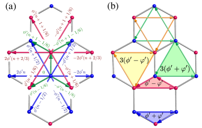
Figure 1: (a) Hopping phases of the Peierls substitution with a Landau gauge $\mathbf{A}=-By\hat{x}$ in the unit cell$(n,m)$. Phases for the NN hopping are in green. Phases for the NNN hopping in sublattices A and B are in red and blue, respectively. Here, $\phi^{\prime}=3\sqrt{3}a^{2}eB/4\hbar.$ (b) Fluxes enclosed by the different paths involving NN and NNN hoppings for positive $B$.

In order to assess the density of states (DOS) and the transverse conductivity of large systems we employ the KPM Weiße et al. (2006), which has been extensively applied to investigate the electronic properties of graphene layers Ferreira et al. (2011a); Fan et al. (2014); Cysne et al. (2016); Leconte et al. (2016). Within this approach the Green’s functions and spectral operators are approximated by accurate matrix polynomial expansions. Chebyshev polynomials of first kind are the most popular choice given their unique convergence properties and relation to the Fourier transform Boyd (2001). The expansion coefficients are computed by means of a highly stable recursive procedure, which allows to treat very large systems sizes. The first step is to rescale the energy spectrum of Eq. (1) into the interval domain $[-1,1]$ of convergence of the spectral series. This is easily achieved by defining rescaled operators and energies variables, that is, $\tilde{H}=(H-b)/a$, and $\tilde{E}=(E-b)/a$, where $a=(E_{T}-E_{B})/(2-\epsilon)$, and $b=(E_{T}+E_{B})/2$. Here, $E_{T}$ and $E_{B}$ denote the top and bottom limits of the energy spectrum, respectively, and $\epsilon$ is a small cut-off parameter introduced to avoid numerical instabilities. To facilicate numerical convergence, we follow Ref. García et al. (2015) and include Anderson disorder in $H$, with on-site energies $\epsilon_{i}$ randomly distributed in $[-\gamma/2,\gamma/2]$.

The DOS of the system is expanded in terms of Chebyshev polynomials $T_{m}(\tilde{E})=\cos(m\arccos(\tilde{E}))$. The $N$-order approximation to the rescaled DOS is

$$\rho(\tilde{E})\simeq\frac{1}{\pi\sqrt{1-\tilde{E}^{2}}}\sum_{m=0}^{N-1}\mu_{m}g_{m}T_{m}(\tilde{E})\,,$$ (2)

where $g_{m}$ is a kernel introduced to damp spurious (Gibbs) oscillations. The Chebyshev moments are obtained from $\mu_{m}=\textrm{Tr}\,\langle T_{m}(\tilde{H})\rangle$, where $\langle...\rangle$ denotes disorder average. To reduce the numerical complexity, we employ the stochastic trace evaluation technique

$$\mu_{m}\simeq\frac{1}{R}\left\langle\sum_{r=1}^{R}\langle\phi_{r}|T_{m}(\tilde{H})|\phi_{r}\rangle\right\rangle\,,$$ (3)

with complex random vectors $|\phi_{r}\rangle=D^{-1/2}\sum_{i=1}^{D}e^{\imath\theta_{i}}|i\rangle$, where $\{|i\rangle\}_{i=1...D}$ is the original site basis and $\theta_{i}$ are independent random phases Weiße et al. (2006). The DOS for strong magnetic fields pointing along the $\pm\hat{z}$ directions is shown in Fig. 2. It reproduces the spectrum of the Haldane model, as expected. The particle-hole symmetry breaking is caused by the inclusion of the next-nearest neighbour hopping integral. Panel (a) shows that the spectrum is only approximately symmetric under reversal of the magnetic field direction. This is clearer in panel (b) depicting a closeup of the DOS around the $n=1,2$ LLs, where a small shift can be appreciated. Although the effect is relatively small, it is not due to numerical inaccuracy. The assymmetry results from competing next-nearest neighbour flux accumulation inside the plaquettes (see Fig. 1) where closed loops connecting sites of sublattice A have different phase variation than the ones connecting sites of sublattice B that depends on the sign of the magnetic field. This difference produces a mismatch between LLs of positive and negative fields and it is responsible for the emergence of SdH oscillations, as we shall subsequently see.

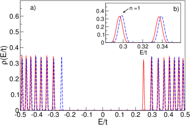
Figure 2: Density of states calculated as a function of energy for a system described by the Haldane model with $2\times 800\times 400$ sites, $t_{2}=\frac{0.5t}{6\sqrt{3}}$, $B=131T$ and $\gamma=0.1t$. The spectral expansion [Eq. (2)] employed $4000$ polynomials and $70$ random vectors. A Jackson kernel was used to damp Gibbs oscillationsWeiße et al. (2006). (a) Plot of the full density of states for positive field configurations (blue dashed line) and negative field configurations (red solid line). (b) Closeup of the DOS around the $n=1$ and $n=2$ LLs.

To calculate the conductivity tensor $\sigma_{\alpha\beta}$, we use an efficient numerical implementation of the KPM developed by García, Covaci and Rappoport García et al. (2015) based on the spectral expansion of the Kubo-Bastin formula Bastin et al. (1971):

$$\sigma_{\alpha\beta}(\mu,T,B)=\frac{\imath e^{2}\hbar}{\Omega}\int_{-\infty}^{\infty}dE\,f(\mu,T,E)$$

$$\times\textrm{Tr}\langle v_{\alpha}\delta(E-H)v_{\beta}\frac{dG^{+}}{dE}-v_{\alpha}\frac{dG^{-}}{dE}v_{\beta}\delta(E-H)\rangle.$$ (4)

In the above, $\mu$, $T$ and $B$ denote the chemical potential, temperature, and applied magnetic field, respectively. The Cartesian components of the velocity operator are designated by $v_{\alpha(\beta)}$, with $\alpha,\beta=x,y$. $G^{\pm}$ stands for the retarded (advanced) single-particle Green’s function and $\delta(E-H)$ is the spectral operator. Finally, $\Omega$ is the area and $f(\mu,T,E)=1/(1+\exp(-(\mu-E)/k_{B}T))$ is the Fermi-Dirac distribution function. The Green’s functions and spectral operators in Eq. (4) are expanded in Chebyshev polynomials as performed for the DOS. Given the large number of moments retained in our calculations, the energy resolution is only limited by the mean level spacing $\delta E$ of the simulated system Leconte et al. (2016); Ferreira and Mucciolo (2015).

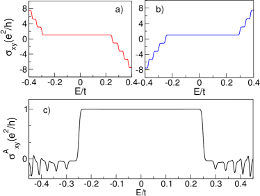
Figure 3: Hall conductivity of the Haldane model calculated as a function of energy. Simulation parameters as in Fig.2. Panels (a) and (b) depict the Hall conductivities calculated for $\vec{B}=\mp B\hat{z}$, respectively, and panel (c) shows the calculated anomalous part of the Hall conductivity.

The anomalous Hall conductivity consists ot two parts: (i) a regular contribution $\sigma_{xy}^{R}$ anti-symmetric with respect to inversion of magnetic field direction and (ii) an anomalous contribution $\sigma_{xy}^{A}$. These are obtained from $\sigma_{xy}^{R(A)}=\frac{1}{2}\left(\sigma_{xy}^{+}\mp\sigma_{xy}^{-}\right)$ with $\sigma_{xy}^{\pm}=\sigma_{xy}(\mu,T,\pm B)$. The results of our simulations are displayed in Fig. 3. The anomalous contribution $\sigma_{xy}^{A}$ to the Hall conductivity is shown in panel (c). The steps in $\sigma_{xy}$ occur whenever the energy crosses a LL (compare with DOS in Fig. 2). The quantized anomalous Hall plateau is clearly visible, however oscillations develop at high electronic density. Upon comparison with the DOS, it becomes clear that the anomalous SdH oscillations are produced by the shift in the spectra for $\vec{B}=\pm B\hat{z}$. These results show that the breaking of electron–hole symmetry has important consequences in the anomalous part of the Hall conductivity.

III Continuum Model

To shed further light onto the anomalous oscillations seen in the quantum transport calculations, we derive a low-energy continuum model. To this end, we expand the tight-binding Hamiltonian Eq. (1) in momentum space around the inequivalent Dirac points $K_{\pm}$ in the Brillouin zoneFerreira et al. (2011a). The magnetic field is included by minimal coupling. We choose the basis $(\mathbf{A},\mathbf{B})^{\textrm{t}}$ for the 4-component spinors with $\mathbf{A}=(A\,K_{+},A\,K_{-})$ (similarly for $\mathbf{B}$). To linear order in $\hbar\delta\mathbf{k}=\hbar(\mathbf{k}-\mathbf{K}_{\pm})$, one obtainsHaldane (1988)

$$H_{\textrm{L.E.}}=v_{F}\left(\tau_{z}\otimes\pi_{x}\otimes\sigma_{x}+\pi_{y}\otimes\sigma_{y}\right)+\Delta\,\tau_{z}\otimes\sigma_{z},$$ (5)

The low-energy Hamoltonian describes the coupling between the momentum of the particles and the pseudo-spin in the long-wavelenght limit. $\vec{\pi}=\hbar\delta\vec{k}-e\vec{A}$ denotes the canonical momentum, $v_{F}=3t_{1}a/2\hbar$ represents the Fermi velocity, $a$ is the lattice constant, and $\tau_{z}=\pm 1$ specifies choice of Dirac point, $\mathbf{K}_{\pm}=\pm(4\pi/3a)\hat{k}_{x}$. Here, $\Delta=3\sqrt{3}t_{2}$ is referred to as the Haldane “mass”. The spectrum reads as

$$E_{n}^{(1)}=\eta\sqrt{\Delta^{2}+2|n|\left(\frac{\hbar v_{F}}{l_{B}}\right)^{2}},\hskip 14.22636pt\text{for $|n|\neq 0\,,$}$$ (6)

$$E_{0}^{(1)}=-s_{B}\Delta,\hskip 14.22636pt\text{for $n=0$.}$$ (7)

$\eta=\pm 1$ for electrons (holes), $s_{B}=\textrm{sign}(B)$ and $l_{B}=(\hbar/e|B|)^{1/2}$ is the magnetic length. $E_{0}^{(1)}$ changes sign when the direction of the applied magnetic field is reversed. However, for $|n|\neq 0$, $E_{n}^{(1)}$ is independent of the field direction, in contrast to the numerical results. This is true for the expansion up to linear order in $\hbar\delta\vec{k}$, but the inclusion of higher order terms can provided further refinements to the LLs energy spectrum Suprunenko et al. (2008); Kretinin et al. (2013). We then include quadratic terms in the low-energy expansion. As far as the shift in the energy spectra for $\vec{B}=\pm\hat{z}$ is concerned, it suffices to consider the correction to the next-nearest neighbours hopping. We find

$$H_{\textrm{L.E.}}^{(2)}=H_{\textrm{L.E.}}-\frac{\boldsymbol{\pi}^{2}}{2m^{\prime}}\,\tau_{z}\otimes\sigma_{z}\,,$$ (8)

with $m^{\prime}=2\hbar^{2}/(t_{2}9\sqrt{3}a^{2})$. The spectrum reads as

$$E_{n\neq 0}^{(2)}=s_{B}\frac{\hbar^{2}}{2m^{\prime}l_{B}^{2}}+\eta\sqrt{\left(\Delta-\frac{\hbar^{2}|n|}{m^{\prime}l_{B}^{2}}\right)^{2}+2|n|\left(\frac{\hbar v_{F}}{l_{B}}\right)^{2}}\,,$$ (9)

$$E_{0}^{(2)}=-s_{B}\left(\Delta-\frac{\hbar^{2}}{2m^{\prime}{l_{B}}^{2}}\right),\hskip 5.69046pt\text{for $n=0$.}$$ (10)

The inclusion of second order terms reproduces the LL shift when the direction of magnetic field is inverted, as found in our numerical simulations: $\Delta E_{n}^{(2)}=E_{n}(|B|)-E_{n}(-|B|)=\hbar^{2}/(2m^{\prime}l_{B}^{2})$ for $|n|\neq 0$ is independent of $n$, and increases linearly with $t_{2}$. The inclusion of quadratic terms in the expansion also reduces the effective contribution from the Haldane “mass” by a factor that increases linearly with $|n|$ for $|n|\neq 0$.

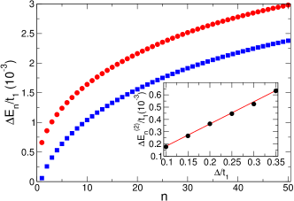
Figure 4: Energy spectra difference $\Delta E_{n}=E_{n}^{(1)}-E_{n}^{(2)}$ calculated for positive (open circle) and negative (solid circles) magnetic field. Inset: Energy spectra shift according to continuum model (blue dashed line) and tight-binding calculations (solid circles). Simulation parameters: $t_{2}=\frac{0.2t}{6\sqrt{3}}$, $D=2\times 10^{6}$ atoms, $|B|=157T$, $N=5000$ and $R=60$.

The difference between the energy spectra in the two approximations is shown in Fig. 4. $\Delta E_{n}$ increases monotonically with $n$ due to the character of the second-order correction in Eq. (8). The dependence of the energy shift with $n$ and $t_{2}$, which is related to the size of the topological gap, can be used to extract the parameters of Chern insulators in transport measurements.

In the inset of Fig. 4 we compare the shifts determined from Eq. (9) with the tight-binding results for different values of the Haldane gap $\Delta=6\sqrt{3}t_{2}$. They are in excellent agreement, showing that shift is a result of deviations from the linear dispersion relation in the vicinity of the Dirac points, arising from competing next-nearest neighbour hopping integral introduced by Haldane and the external magnetic field.

IV Anomalous Oscillations

The continuum model can provide crucial information on the anomalous Hall conductivity for realistic magnetic fields not accessible with our KPM implementation. For this purpose, we evaluate the transverse conductivity $\sigma_{xy}$ within the empty-bubble approximation Tsaran and Sharapov (2016); Ferreira et al. (2011b)

$$\sigma_{xy}=\frac{e^{2}\hbar}{2\pi\imath\,l_{B}^{2}}\,\sum_{n\neq m}\,\frac{\langle v_{x}\rangle_{nm}\langle v_{y}\rangle_{mn}}{\delta E_{nm}^{(2)}\,(\delta E_{nm}^{(2)}+\imath\gamma)}\,\delta f_{nm}(\mu,T)\,,$$ (11)

where $E_{nm}^{(2)}=E_{n}^{(2)}-E_{m}^{(2)}$, $\delta f_{nm}$ is the respective difference of occupation factors and $\gamma$ is a broadening parameter. The velocity matrix elements for states around $K_{+}$ are

$$\langle v_{x}\rangle_{nm}=v_{F}N_{n,m}[\alpha_{n}\delta_{|n|,|m|-1}+\alpha_{m}\delta_{|n|-1,|m|}]\,,$$ (12)

$$\langle v_{y}\rangle_{mn}=iv_{F}N_{n,m}[-\alpha_{n}\delta_{|m|-1,|n|}+\alpha_{m}\delta_{|m|,|n|-1}]\,,$$ (13)

with

$$\alpha_{n}=\frac{{E_{n}^{(2)}}-s_{B}\frac{\hbar^{2}}{2m^{\prime}l_{B}^{2}}-\Delta+\frac{\hbar^{2}|n|}{{l_{B}}^{2}m^{\prime}}}{\sqrt{2|n|}\frac{\hbar v_{F}}{l_{B}}}\,,$$ (14)

$$N_{nm}=\frac{1}{\sqrt{1+\left({\alpha_{n}}\right)^{2}}}\frac{1}{\sqrt{1+\left({\alpha_{m}}\right)^{2}}}.$$ (15)

Figure 5 shows the predicted anomalous Hall conductivity at 10 T for selected temperatures, using indicative values of hopping integrals motivated by a realization with graphene, that is, $t_{1}=3$ eV and $t_{2}=3\times 10^{-2}$ eV. For example, a Chern insulator could be induced in graphene by proximity effect with either monolayer T’-WTe in combination with a ferromagnetic insulator or magnetic doped T’-WTe. The WTe monolayer provides the quantum spin Hall state Wu et al. (2018) and the spin degeneracy is lifted by a ferromagnetic layer Wei et al. (2016). The effect is less visible at higher temperatures due to the smearing of the quantum Hall steps. It is noteworthy that these SdH oscillations have a different origin from those discussed in Ref. Tsaran and Sharapov, 2016, which manifest in the valley or spin Hall conductivity and thus require measurements of the nonlocal resistanceGorbachev et al. (2014). We deal with a different model system, which in the absence of a magnetic field is a Chern insulator with Chern number $C=1$. Here, the renormalized Haldane “mass” has opposite signs at $K_{\pm}$ and leads to a Hall conductivity $\sigma_{xy}\neq 0$ for $B=0$. The predicted anomalous SdH oscillations should manifest in charge transport measurements of $\sigma_{xy}(\mu,T,\pm B)$.

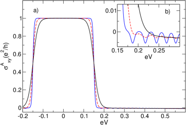
Figure 5: (a) Anomalous part of the Hall conductivity calculated for the Haldane model in the continuum limit, including second order corrections. Results are obtained for $t_{2}\approx 0.03$ eV, $|B|=10$ T, $\Gamma=0.3$ meV, and different temperatures: $T=35$ K (blue solid line), $T=70$ K (red dashed line), and $T=140$ K (black solid line). Panel (b) highlights the SdH oscillations in the anomalous part of the Hall conductivity

V Conclusions

We have investigated the transport properties of the Haldane model in presence of strong magnetic fields by means of real-space calculations and low-energy continuum models. We identified in our numerical calculations a displacement between the energy spectra for magnetic fields of opposite directions, verifying that the Landau levels for $|n|\neq 0$ are only approximately symmetric with respect to inversion of the applied magnetic field $B\rightarrow-B$. The mismatch between the LLs of positive and negative magnetic fields leads to SdH oscillations in the anomalous contribution to the Hall conductivity, which can be observed even at liquid nitrogen temperatures for Chern insulators with large topological gaps. The presence of the quantum magneto-oscillations in the anomalous contribution to the Hall conductivity arises as a direct consequence of competing neighbour flux accumulation due to broken TRS. Therefore, we expect this phenomenon to be present in systems that exhibit an anomalous Hall state, such as magnetic topological insulators, where the TRS is broken by magnetic ordering Chang et al. (2013, 2015); Kim et al. (2017); Bestwick et al. (2015); Zou et al. (2017). Furthermore, these oscillations could be used as a tool to extract properties of the underlying microscopic mechanism that creates the energy gap in the system, such as the next-nearest neighbor amplitude in the Haldane modelHaldane (1988) or the tunneling amplitude between surface states of thin films mediated by spin–orbit coupling Yu et al. (2010); Zhang et al. (2010); Kou et al. (2015). The recent observation of quantum spin Hall effect in two-dimensional WTe₂ at temperatures of up to 100K Sanfeng Wu et al. (2018) hints at a possible route for the fabrication of magnetic topological insulators with large topological gaps, where SdH oscillations in the anomalous contribution to Hall conductivity as described in this work could be observed.

We acknowledge the Brazilian agencies CAPES and CNPq for financial support. T.G.R. and A.F. acknowledge support from the Newton Fund and the Royal Society through the Newton Advanced Fellowship scheme (Ref. NA150043). J.H.G. received funding from the European Unions Horizon 2020 research and innovation programme under grant agreement No 696656 (Graphene Flagship). ICN2 is supported by the Severo Ochoa program from Spanish MINECO (Grant No. SEV-2013-0295) and funded by the CERCA Programme / Generalitat de Catalunya.

References

- Klitzing et al. [1980] K. v. Klitzing, G. Dorda, and M. Pepper, Phys. Rev. Lett. 45, 494 (1980), URL http://link.aps.org/doi/10.1103/PhysRevLett.45.494.
- Thouless et al. [1982] D. J. Thouless, M. Kohmoto, M. P. Nightingale, and M. den Nijs, Phys. Rev. Lett. 49, 405 (1982), URL http://link.aps.org/doi/10.1103/PhysRevLett.49.405.
- Streda [1982] P. Streda, Journal of Physics C: Solid State Physics 15, L1299 (1982), URL http://stacks.iop.org/0022-3719/15/i=36/a=006.
- Simon [1983] B. Simon, Phys. Rev. Lett. 51, 2167 (1983), URL http://link.aps.org/doi/10.1103/PhysRevLett.51.2167.
- Berry [1984] M. V. Berry, Proceedings of the Royal Society of London A: Mathematical, Physical and Engineering Sciences 392, 45 (1984), ISSN 0080-4630, URL http://rspa.royalsocietypublishing.org/content/392/1802/45.
- Haldane [1988] F. D. M. Haldane, Phys. Rev. Lett. 61, 2015 (1988), URL http://link.aps.org/doi/10.1103/PhysRevLett.61.2015.
- Semenoff [1984] G. W. Semenoff, Phys. Rev. Lett. 53, 2449 (1984), URL http://link.aps.org/doi/10.1103/PhysRevLett.53.2449.
- Novoselov et al. [2004] K. S. Novoselov, A. K. Geim, S. V. Morozov, D. Jiang, Y. Zhang, S. V. Dubonos, I. V. Grigorieva, and A. A. Firsov, Science 306, 666 (2004).
- Kane and Mele [2005a] C. L. Kane and E. J. Mele, Phys. Rev. Lett. 95, 226801 (2005a), URL https://link.aps.org/doi/10.1103/PhysRevLett.95.226801.
- Kane and Mele [2005b] C. L. Kane and E. J. Mele, Phys. Rev. Lett. 95, 146802 (2005b), URL https://link.aps.org/doi/10.1103/PhysRevLett.95.146802.
- Hasan and Kane [2010] M. Z. Hasan and C. L. Kane, Rev. Mod. Phys. 82, 3045 (2010), URL http://link.aps.org/doi/10.1103/RevModPhys.82.3045.
- Chang et al. [2013] C.-Z. Chang, J. Zhang, X. Feng, J. Shen, Z. Zhang, M. Guo, K. Li, Y. Ou, P. Wei, L.-L. Wang, et al., Science 340, 167 (2013), ISSN 0036-8075, URL http://science.sciencemag.org/content/340/6129/167.
- Jotzu et al. [2014] G. Jotzu, M. Messer, R. Desbuquois, M. Lebrat, T. Uehlinger, D. Greif, and T. Esslinger, Nature 515, 237 (2014), ISSN 0028-0836, letter, URL http://dx.doi.org/10.1038/nature13915.
- Wright [2013] A. R. Wright, Scientific Reports 3, 2736 EP (2013), URL http://dx.doi.org/10.1038/srep02736.
- Wang et al. [2015a] Z. Wang, D. Ki, H. Chen, H. Berger, A. H. MacDonald, and A. F. Morpurgo, Nat. Commun. 6, 8339 (2015a), ISSN 2041-1723, eprint 1508.02912, URL http://www.nature.com/doifinder/10.1038/ncomms9339.
- Benítez et al. [2017] L. A. Benítez, J. F. Sierra, W. Savero Torres, A. Arrighi, F. Bonell, M. V. Costache, and S. O. Valenzuela, Nat. Phys. (2017), ISSN 1745-2473, eprint arXiv:1710.11568, URL http://www.nature.com/articles/s41567-017-0019-2.
- Ghiasi et al. [2017] T. S. Ghiasi, J. Ingla-Aynés, A. A. Kaverzin, and B. J. van Wees, Nano Lett. p. acs.nanolett.7b03460 (2017), ISSN 1530-6984, eprint 1708.04067, URL https://arxiv.org/pdf/1708.04067.pdfhttp://arxiv.org/abs/1708.04067http://pubs.acs.org/doi/10.1021/acs.nanolett.7b03460.
- Wang et al. [2015b] Z. Wang, C. Tang, R. Sachs, Y. Barlas, and J. Shi, Phys. Rev. Lett. 114, 016603 (2015b), URL https://link.aps.org/doi/10.1103/PhysRevLett.114.016603.
- Hallal et al. [2017] A. Hallal, F. Ibrahim, H. Yang, S. Roche, and M. Chshiev, 2D Mater. 4, 025074 (2017), ISSN 2053-1583, URL http://stacks.iop.org/0957-4484/28/i=45/a=455706?key=crossref.c18830a50f5d5652f7676e2b7f076cffhttp://stacks.iop.org/2053-1583/4/i=2/a=025074?key=crossref.f09e7cc93c243fbc5a683800d741d202.
- Phong et al. [2018] V. T. Phong, N. R. Walet, and F. Guinea, 2D Materials 5, 014004 (2018), URL http://stacks.iop.org/2053-1583/5/i=1/a=014004.
- Tsaran and Sharapov [2016] V. Y. Tsaran and S. G. Sharapov, Phys. Rev. B 93, 075430 (2016), URL http://link.aps.org/doi/10.1103/PhysRevB.93.075430.
- Silver and Röder [1997] R. N. Silver and H. Röder, Phys. Rev. E 56, 4822 (1997), URL http://link.aps.org/doi/10.1103/PhysRevE.56.4822.
- Weiße et al. [2006] A. Weiße, G. Wellein, A. Alvermann, and H. Fehske, Rev. Mod. Phys. 78, 275 (2006), URL http://link.aps.org/doi/10.1103/RevModPhys.78.275.
- García et al. [2015] J. H. García, L. Covaci, and T. G. Rappoport, Phys. Rev. Lett. 114, 116602 (2015), URL http://link.aps.org/doi/10.1103/PhysRevLett.114.116602.
- Ferreira et al. [2011a] A. Ferreira, J. Viana-Gomes, J. Nilsson, E. R. Mucciolo, N. M. R. Peres, and A. H. Castro Neto, Phys. Rev. B 83, 165402 (2011a), URL https://link.aps.org/doi/10.1103/PhysRevB.83.165402.
- Fan et al. [2014] Z. Fan, A. Uppstu, and A. Harju, Phys. Rev. B 89, 245422 (2014), URL https://link.aps.org/doi/10.1103/PhysRevB.89.245422.
- Cysne et al. [2016] T. P. Cysne, T. G. Rappoport, A. Ferreira, J. M. V. P. Lopes, and N. M. R. Peres, Phys. Rev. B 94, 235405 (2016), URL https://link.aps.org/doi/10.1103/PhysRevB.94.235405.
- Leconte et al. [2016] N. Leconte, A. Ferreira, and J. Jung, in 2D Materials, edited by F. Iacopi, J. J. Boeckl, and C. Jagadish (Elsevier, 2016), vol. 95 of Semiconductors and Semimetals, pp. 35 – 99, URL http://www.sciencedirect.com/science/article/pii/S0080878416300047.
- Boyd [2001] J. P. Boyd, Chebyshev and Fourier Spectral Methods, Dover Books on Mathematics (Dover Publications, Mineola, NY, 2001), 2nd ed., ISBN 0486411834 9780486411835.
- Bastin et al. [1971] A. Bastin, C. Lewiner, O. Betbedermatibet, and P. Nozieres, Journal of Physics and Chemistry of Solids 32, 1811 (1971).
- Ferreira and Mucciolo [2015] A. Ferreira and E. R. Mucciolo, Phys. Rev. Lett. 115, 106601 (2015), URL https://link.aps.org/doi/10.1103/PhysRevLett.115.106601.
- Suprunenko et al. [2008] Y. F. Suprunenko, E. V. Gorbar, V. M. Loktev, and S. G. Sharapov, Low Temperature Physics 34, 812 (2008), eprint http://dx.doi.org/10.1063/1.2981394, URL http://dx.doi.org/10.1063/1.2981394.
- Kretinin et al. [2013] A. Kretinin, G. L. Yu, R. Jalil, Y. Cao, F. Withers, A. Mishchenko, M. I. Katsnelson, K. S. Novoselov, A. K. Geim, and F. Guinea, Phys. Rev. B 88, 165427 (2013), URL http://link.aps.org/doi/10.1103/PhysRevB.88.165427.
- Ferreira et al. [2011b] A. Ferreira, J. Viana-Gomes, Y. V. Bludov, V. Pereira, N. M. R. Peres, and A. H. Castro Neto, Phys. Rev. B 84, 235410 (2011b), URL http://link.aps.org/doi/10.1103/PhysRevB.84.235410.
- Wu et al. [2018] S. Wu, V. Fatemi, Q. D. Gibson, K. Watanabe, T. Taniguchi, R. J. Cava, and P. Jarillo-Herrero, Science 359, 76 (2018), ISSN 0036-8075, eprint http://science.sciencemag.org/content/359/6371/76.full.pdf, URL http://science.sciencemag.org/content/359/6371/76.
- Wei et al. [2016] P. Wei, S. Lee, F. Lemaitre, L. Pinel, D. Cutaia, W. Cha, F. Katmis, Y. Zhu, D. Heiman, J. Hone, et al., Nature Materials 15, 711 EP (2016), URL http://dx.doi.org/10.1038/nmat4603.
- Gorbachev et al. [2014] R. V. Gorbachev, J. C. W. Song, G. L. Yu, A. V. Kretinin, F. Withers, Y. Cao, A. Mishchenko, I. V. Grigorieva, K. S. Novoselov, L. S. Levitov, et al., Science 346, 448 (2014), ISSN 0036-8075, eprint http://science.sciencemag.org/content/346/6208/448.full.pdf, URL http://science.sciencemag.org/content/346/6208/448.
- Chang et al. [2015] C.-Z. Chang, W. Zhao, D. Y. Kim, H. Zhang, B. A. Assaf, D. Heiman, S.-C. Zhang, C. Liu, M. H. W. Chan, and J. S. Moodera, Nature Materials 14, 473 (2015), ISSN 1476-1122, URL http:https://doi.org/10.1038/nmat4204.
- Kim et al. [2017] J. Kim, S.-H. Jhi, A. H. MacDonald, and R. Wu, Phys. Rev. B 96, 140410 (2017), URL https://link.aps.org/doi/10.1103/PhysRevB.96.140410.
- Bestwick et al. [2015] A. J. Bestwick, E. J. Fox, X. Kou, L. Pan, K. L. Wang, and D. Goldhaber-Gordon, Phys. Rev. Lett. 114, 187201 (2015), URL https://link.aps.org/doi/10.1103/PhysRevLett.114.187201.
- Zou et al. [2017] W. Zou, W. Wang, X. Kou, M. Lang, Y. Fan, E. S. Choi, A. V. Fedorov, K. Wang, L. He, Y. Xu, et al., Applied Physics Letters 110, 212401 (2017), eprint https://doi.org/10.1063/1.4983684, URL https://doi.org/10.1063/1.4983684.
- Yu et al. [2010] R. Yu, W. Zhang, H.-J. Zhang, S.-C. Zhang, X. Dai, and Z. Fang, Science 329, 61 (2010), ISSN 0036-8075, URL http://science.sciencemag.org/content/329/5987/61.
- Zhang et al. [2010] Y. Zhang, K. He, C.-Z. Chang, C.-L. Song, L.-L. Wang, X. Chen, J.-F. Jia, Z. Fang, X. Dai, W.-Y. Shan, et al., Nature Physics 6, 584 (2010), ISSN 1745-2473, URL http:https://doi.org/10.1038/nphys1689.
- Kou et al. [2015] X. Kou, L. Pan, J. Wang, Y. Fan, E. S. Choi, W.-L. Lee, T. Nie, K. Murata, Q. Shao, S.-C. Zhang, et al., Nature Communications 6, 8474 (2015), ISSN 2041-1733, URL http:https://doi.org/10.1038/ncomms9474.
- Sanfeng Wu et al. [2018] V. F. Sanfeng Wu, Q. D. Gibson, K. Watanabe, T. Taniguchi, R. J. Cava, and P. Jarillo-Herrero, Science 359, 76 (2018).