Color screening in (2+1)-flavor QCD
Abstract
We study correlation functions of spatially separated static quark-antiquark pairs in (2+1)-flavor QCD in order to investigate onset and nature of color screening at high temperatures. We perform lattice calculations in a wide temperature range, , using the highly improved staggered quark action and several lattice spacings to control discretization effects. By comparing at high temperatures our lattice results to weak-coupling calculations as well as to the zero temperature result for the energy of a static quark-antiquark pair, we observe that color screening sets in at . Furthermore, we also observe that in the range weak-coupling calculations in the framework of suitable effective field theories provide an adequate picture of color screening.
pacs:
12.38.Gc, 12.38.-t, 12.38.Bx, 12.38.MhI Introduction
As the temperature of strongly interacting matter increases to a pseudocritical temperature , a transition to a state with different properties than the vacuum at zero temperature occurs. Deconfinement of gluons and quarks, restoration of chiral symmetry and screening of color charges are key properties of this thermal medium (cf. recent reviews, e.g. Bazavov (2015); Petreczky (2012); Ding et al. (2015a)).
For pure Yang-Mills theory (SU() gauge theory), the Polyakov loop and the correlator of two Polyakov loops are the order parameters of the deconfinement transition, in which the center symmetry McLerran and Svetitsky (1981); Kuti et al. (1981) of the pure Yang-Mills vacuum is broken. Since the center symmetry is broken by dynamical quarks already at zero temperature, neither the Polyakov loop nor the Polyakov loop correlator are order parameters of full QCD Bazavov et al. (2009, 2012). Nevertheless, the Polyakov loop correlator is a sensitive probe of deconfinement and color screening. In particular, it provides insight into the intricate screening properties of the thermal medium. The properly renormalized correlator of two Polyakov loops is related to the free energy of a static quark-antiquark () pair at separation and temperature McLerran and Svetitsky (1981); Kaczmarek et al. (2002),
| (1) |
We choose to renormalize in such a way that for infinite separation matches the sum of the free energies of a decoupled static quark and antiquark using the renormalization of Ref. Bazavov et al. (2016). This is the same renormalization scheme that is usually used for matching the static energy at zero temperature for different lattice spacings.
Polyakov loop correlators have been calculated on the lattice for a long time. Calculations have been performed in SU(2) gauge theory Irback et al. (1991); LaCock et al. (1992); Datta and Gupta (2000); Fiore et al. (2003); Digal et al. (2003); Bazavov et al. (2008) and SU(3) gauge theory Karkkainen et al. (1992); Kaczmarek et al. (2000); Petreczky et al. (2002); Kaczmarek et al. (2002); Akerlund and de Forcrand (2014) as well as in QCD with two quark flavors Detar et al. (1999); Karsch et al. (2001); Kaczmarek and Zantow (2005) and three quark flavors Petreczky and Petrov (2004). More recent calculations of the Polyakov loop correlator and of the color singlet correlator have been performed with (2+1) dynamical flavors of sea quarks using different types of staggered quark formulations at or close to the physical point Petreczky (2010); Bazavov and Petreczky (2013a); Borsanyi, Szabolcs and Fodor, Zoltan and Katz, Sándor D. and Pásztor, Attila and Szabó, Kálmán K. and Török, Csaba (2015). In Ref. Borsanyi, Szabolcs and Fodor, Zoltan and Katz, Sándor D. and Pásztor, Attila and Szabó, Kálmán K. and Török, Csaba (2015) results in the continuum limit have been presented. Very recently the Polyakov loop correlators have been calculated at nonzero baryon density Andreoli et al. (2018).
At sufficiently high temperatures and short distances, the Polyakov loop correlators can be calculated using the weak-coupling expansion, i.e. the expansion in the gauge coupling . In this regime, besides the scale and the Coulomb potential , there are three relevant thermodynamical scales that need to be considered: , (electric mass) and (also called the magnetic mass). The leading order weak-coupling result for the Polyakov loop correlator has been known for a long time Gross et al. (1981); McLerran and Svetitsky (1981) and implies a non-Coulombic behavior of the static free energy due to the cancellation of the singlet and octet contributions Gross et al. (1981); McLerran and Svetitsky (1981). The next-to-leading-order calculation of the Polyakov loop correlator was performed by Nadkarni in the large distance regime, Nadkarni (1986), whereas the corresponding calculation in the short distance regime, , has been performed relatively recently Brambilla et al. (2010). In Berwein et al. (2017) one can find the state of the art expression for the Polyakov loop correlator at short distances, which is valid up to order and in the multipole expansion. In this regime it turns out to be useful to organize the calculation by means of the effective field theory called potential nonrelativistic QCD (pNRQCD) Pineda and Soto (1998); Brambilla et al. (2000, 2005). For distances the behavior of the Polyakov loop correlator can be best understood in the framework of the dimensionally reduced effective field theory called electrostatic QCD (EQCD) Braaten and Nieto (1996) (see references therein for related works). At very large distances, , the perturbative expansion breaks down due to the well-known Linde problem Linde (1980). In Refs. Rebhan (1994); Braaten and Nieto (1994), using EQCD, it was shown indeed that the very large distance behavior of the Polyakov loop correlator is affected by chromomagnetic screening and its correct asymptotic behavior is given by the lowest glueball mass at high temperatures Braaten and Nieto (1995); Arnold and Yaffe (1995). The screening mass that governs the large distance behavior of the Polyakov loop correlator has been calculated in EQCD using lattice techniques and also investigated with weak-coupling methods in Laine and Vepsalainen (2009).
Most of the lattice QCD studies have focused on the large distance behavior of the Polyakov loop correlators and the extraction of the corresponding screening masses. The aim of this paper is to study the Polyakov loop correlator from small to large distances and see in what temperature and distance regime contact to weak-coupling calculations can be made. Such an analysis will also help to clarify at which distances color screening effects set in. As it was pointed out in the past, for understanding the temperature behavior of the Polyakov loop correlator it is useful to consider the singlet correlator Kaczmarek et al. (2002); Brambilla et al. (2010). Therefore in this paper we will also present a detailed study of the singlet correlator and its comparison to weak-coupling calculations Burnier et al. (2010); Berwein et al. (2017).
The question of the onset of color screening and applicability of weak-coupling expressions to the Polyakov loop and singlet correlators is not only of academic interest. There is an ongoing theoretical effort to understand quarkonium production in heavy-ion collisions (see e.g. Refs. Mocsy et al. (2013); Blaizot and Escobedo (2017)), which requires the knowledge of in-medium quarkonium properties. Full QCD lattice determinations of in-medium quarkonium properties turn out to be difficult (see, e.g., Refs. Wetzorke et al. (2002); Datta et al. (2004)), which leads to the use of effective field theories Burnier et al. (2008); Brambilla et al. (2008); Petreczky et al. (2011); Burnier et al. (2015, 2016); Brambilla et al. (2017, 2018). Those, on the other hand require one to know which scale hierarchy is relevant for the physically interesting case. The analysis presented in this paper aims at shedding some light on this issue.
The rest of the paper is organized as follows. In Sec. II, we cover technicalities of the lattice simulations. In Sec. III, we present our numerical results, the extraction of the continuum limit, and discuss some general features of the studied correlators, which do not require reference to explicit weak-coupling expressions. In the following two Secs. IV and V, we conduct a systematic and quantitative comparison of the lattice results with the predictions from weak-coupling calculations. We finally use this knowledge for a discussion of the regime of asymptotic screening in Sec. VI. The last section of the paper contains our conclusions. Many technical details of the calculations are discussed in the Appendixes. Some preliminary results from the present study have been reported in conference proceedings Weber et al. (2016); Petreczky and Weber (2016); Weber (2017).
II Lattice QCD Setup and renormalization
We perform calculations of the Polyakov loop correlator as well as of the singlet correlator of static in (2+1)-flavor QCD at nonzero temperature on lattices with , and and aspect ratios of and using the highly improved staggered quark (HISQ) action Follana et al. (2007). The calculations have been performed at the physical value of the strange quark mass and the light quark masses . The latter corresponds to a pion mass of in the continuum limit. We performed calculations in a wide beta range with being the lattice bare gauge coupling. The lattice spacing has been fixed by the scale and we use the parametrization of given in Ref. Bazavov et al. (2014a). Using this parametrization we find that the above range corresponds to a temperature range of . The gauge configurations used in this study have been generated by the HotQCD Collaboration Bazavov et al. (2012, 2014a). We also used the gauge configurations generated by the study of quark number susceptibilities at high temperatures Ding et al. (2015b); Bazavov et al. (2013). Additional gauge configurations have been generated specifically for this study. Some of these gauge configurations have been used in the study of the renormalized Polyakov loop with the HISQ action Bazavov and Petreczky (2013b); Bazavov et al. (2016). A detailed account of the used gauge configurations, including the new gauge configurations by our (TUMQCD) collaboration is presented in Appendix A. Furthermore, in the high temperature region MeV additional gauge configurations have been generated with , and , for , and and light quark mass . This light quark mass corresponds to a pion mass of in the continuum limit. The aim of these calculations was to extend the continuum results on the correlators to higher temperatures. For temperatures MeV, quark mass effects are expected to be negligible. We checked this explicitly in Appendix A. Finally, to study finite size effects for the large distance behavior of the correlators, we generated additional gauge configurations on lattices (see Appendix A).
We have generated the new gauge ensembles using the rational hybrid Monte-Carlo (RHMC) algorithm and the MILC Collaboration code. Details on the HISQ action implementation in the MILC code can be found in Ref. Bazavov et al. (2010).
In this paper, we study the correlation functions of the Polyakov loop. The (bare) Polyakov loop is defined in lattice QCD as the normalized trace of a temporal Wilson line wrapping around the time direction once,
| (2) | ||||
| (3) |
where are the temporal link variables. We denote the expectation value of the bare Polyakov loop averaged over the spatial lattice volume as
| (4) |
The bare Polyakov loop correlator is defined as the ensemble average (spatial average over included)
| (5) |
The superscript “bare” refers to the fact that the quantity is not renormalized. In addition we study the singlet correlator in the Coulomb gauge Kaczmarek et al. (2002); Digal et al. (2003), defined as
| (6) |
as well as the cyclic Wilson loops Jahn and Philipsen (2004); Bazavov et al. (2008); Berwein et al. (2013)
where is a spatial Wilson line between the points and . These quantities can be considered as meson correlation functions composed of a static quark and antiquark separated by a distance Jahn and Philipsen (2004); Bazavov et al. (2008) and evaluated at Euclidean time Jahn and Philipsen (2004); Bazavov et al. (2008). The subscript bare refers again to the fact that these are unrenormalized quantities. At very large distances , and approach in the infinite volume limit Kaczmarek et al. (2002); Bazavov et al. (2008); Bazavov and Petreczky (2013c).111Here we take into account that in QCD is real. These bare quantities contain ultraviolet (UV) divergences that are regularized on the lattice. The continuum limit requires looking for combinations of bare quantities that are free of UV divergences.
The renormalization of is simple: the only divergences here are the ones associated with the two Polyakov loops. Therefore, the normalized Polyakov loop correlator
| (7) |
is free of UV divergences and the continuum limit can be taken. In particular, this implies that Eq. (7) can be written directly in terms of renormalized quantities, namely,
| (8) |
where is the renormalized Polyakov loop correlator and is the renormalized Polyakov loop. The normalized Polyakov loop correlator is simply the connected part of the Polyakov loop correlator and contains the complete information about the in-medium modification of the interaction. The disconnected part of the renormalized correlator, i.e. , contains information about infinitely separated static quarks or antiquarks that interact exclusively with the medium, but not with each other.
A similar observation holds for the singlet correlator and we can use the normalized correlation function also in this case,
| (9) |
The above expression, which is defined in the Coulomb gauge, is free of divergences and has a well-defined continuum limit. Such a statement does not hold for general gauges: in covariant gauges, the normalized correlator will be UV divergent Burnier et al. (2010). Another reason for using the Coulomb gauge is that weak-coupling calculations are available in this case Brambilla et al. (2010); Burnier et al. (2010); Berwein et al. (2017).
Since the normalized Polyakov loop and singlet correlators are ultraviolet finite, we can define the subtracted free energy of a static pair and the so-called (subtracted) singlet free energy by taking the logarithm of these correlators,
| (10) | ||||
| (11) |
Here we have traded and for the physical temperature and the lattice spacing . Up to a finite constant, Eqs. (1) and (10) define the same free energy. From Eq. (8), it follows that this constant is given by . The expectation value of the renormalized Polyakov loop is related to the free energy of an isolated static quark at temperature ,
| (12) |
The constant is therefore the free energy of two static quarks or antiquarks that are at infinite separation and, thus, can only interact with the medium. The regularized UV divergence of is exactly the square root of the regularized UV divergence of or . Hence, by adding twice the free energy of an isolated static quark , determined in Ref. Bazavov et al. (2016), we get the free energy of a static pair as well as the singlet free energy,
| (13) | ||||
| (14) |
Equation (13) trivially follows from Eqs. (1), (8), (10), and (12). Equation (14) is the analog for the singlet free energy. Thus, the problem of renormalizing the Polyakov loop and singlet correlators is reduced to the problem of renormalizing . For the latter, we use the procedure described in Ref. Bazavov et al. (2016) and update it with the most recent lattice results. The updated renormalization of is presented in Appendix A. The above procedure also turns out to be very convenient when performing the continuum extrapolations discussed in the next section.
Another way to study in-medium modifications of the interaction of static quark and antiquark is to consider cyclic Wilson loops Jahn and Philipsen (2004); Bazavov et al. (2008); Bazavov and Petreczky (2013c); Berwein et al. (2014). The renormalization of the cyclic Wilson loops, however, is more complicated. In this case, in addition to the self-energy divergences present in the Polyakov loop correlators, there are also self-energy divergences associated with the spatial Wilson lines and , as well as intersection divergences Berwein et al. (2013). On the lattice there are also cusp divergences for off-axis separations. Rectangular Wilson loops evaluated for have cusp divergences at the four corners of the loop. These cusp divergences are absent for cyclic Wilson loops (i.e. for ) in the continuum, because the corresponding contour is smooth. However, on the lattice, one can also consider cyclic Wilson loops for noninteger multiples of the lattice spacing by using Wilson lines that are not aligned with any of the spatial lattice axes. Such off-axis spatial separations, e.g., , involve cusps. In other words, for off-axis separation, the cyclic Wilson loops have additional cusp divergences, while for on-axis separation, such divergences are absent. To simplify the analysis, we only consider on-axis separation. Constructing the spatial part of the cyclic Wilson loops from the smeared gauge links can reduce the size of the UV divergences. Therefore, we calculate the cyclic Wilson loops with spatial lines obtained from smeared gauge links. We apply several steps of hypercubic (HYP) smearing Hasenfratz and Knechtli (2001) and use the same parameters for HYP smearing as in Ref. Hasenfratz and Knechtli (2001).
III Lattice results
In this section, we discuss the dependence of the Polyakov loop correlator, defined in Eq. (5) and the singlet correlator, given in Eq. (6), on the separation of the static quark-antiquark pair at different temperatures. The lattice results for the Polyakov loop correlator and the singlet correlator are functions of three variables: the distance , the lattice spacing , and the temporal extent . The temperature is related to and through ; by trading for the temperature , we parametrize cutoff effects by the dependence of the correlators at fixed temperature. In total, we analyze a full set of more than 10000 data (expectation values) from more than 150 gauge ensembles. The temperature range covers the confined phase, the crossover region, and a strongly as well as weakly coupled quark-gluon plasma phase. The separation range covers asymptotic freedom at short and color screening at large distances.
III.1 Outline of the analysis
The correlator data for different are available only for heterogeneous sets of temperatures and for heterogeneous sets of separations at each temperature. Therefore, the comparison of correlators obtained for different and eventually the continuum extrapolation requires either a three-dimensional, fully global fit or, in one way or another, an interpolation in the separation (or in ) and in the temperature using smoothing functions in order to obtain an intermediate, homogeneously spaced grid of mock data. We perform separate fits in the separation and the temperature sequentially (local fits) or simultaneous fits in the separation and the temperature (global fits). Smoothness in both separation and temperature is a physical constraint in the absence of sharp phase transitions, but inevitably leads to a shrinkage of the errors in the process. Hence, we have to expect that errors of the mock data may be underestimated.
Since no analytic results are available that cover the whole range spanned by the available lattice data, any interpolation introduces some degree of bias. In order to minimize this bias, we identify classes of apparently sensible model functions. For small separations, such model functions are constrained by asymptotic freedom and expectations based on the leading-order weak-coupling results. For larger separations, such model functions are constrained by the dominance of massive one-particle exchange processes, i.e. exponential damping due to color screening. We do not enforce exponential damping for lower temperatures, arguing that confinement may still be unabated or that we may fail to resolve the damping due to a lack of data with sufficient accuracy at large enough separations. For even larger separations, subtracted free energies must approach zero due to cluster decomposition, unless statistical fluctuations (for smaller ensembles) or artifacts of the finite volume lead to an incomplete cancellation and, thus, to a constant value. We account for all of these effects in the interpolations discussed in Appendix C and use a data-driven procedure to identify the most adequate (i.e. most simple) interpolating functions. We note that in the case of we actually find that the lattice data successfully override our inherent bias at low temperatures. Namely, we identify Coulombic interactions despite our explicit bias towards non-Coulombic interactions (see the discussion in Sec. III.3).
As ensembles at different temperature (or at different ) are statistically independent, correlated fluctuations that affect the size of error estimates are relevant only for an interpolation in the separation. Since we are interested in the behavior of the correlators in a wide range of distances , down to the shortest ones, it is important to take care of the lattice artifacts present at short distances before performing the interpolation in . To do this, we utilize the results of the lattice calculation of the static energy at zero temperature (published in Refs. Bazavov et al. (2014a, 2018) and the procedure described in Ref. Bazavov et al. (2014b)). We give a detailed account of the underlying procedure in Appendix B. When discussing the static energy throughout this section, we always use these nonperturbatively improved lattice results. This improvement procedure, however, introduces systematical uncertainties at short distances that we have to estimate heuristically. Such systematical uncertainties are manifestly uncorrelated and orders of magnitude larger than the corresponding statistical errors. That is why the total uncertainties of the data underlying the interpolations (including short distances) are always dominated by uncorrelated errors. Hence, uncorrelated fits aiming for are an appropriate procedure for analyzing these data, where represents degrees of freedom.
We generalize the improvement procedure to correlators with . Here, in particular, for ensembles with smaller , we have to be aware that medium effects may become important in the short distance range, where we apply the nonperturbative improvement. For this reason, we have to expect that we may very well underestimate the associated uncertainties and account for this by enlarging the errors if we cannot interpolate smoothly between data at short distances with . After correcting for short distance lattice artifacts we perform interpolations of and in and using splines or polynomial fits with exponentially decaying prefactor of the form , where is a fit parameter. We perform uncorrelated fits on the individual jackknife bins and determine the errors of the fit from the respective variance of the fit model. These interpolations are only weakly constrained for the largest separations.
In a secondary interpolation at fixed , we use in the absence of justified model assumptions, smoothing splines to interpolate the mock data in using uncorrelated fits, since ensembles at different are statistically independent. Correlators at lower temperatures usually have consistently larger uncertainties than correlators at higher temperatures. For this reason, we have to separately fit in overlapping low and high temperature ranges in order to be sensitive to the lower temperatures. As we typically have about 30 different temperatures for each , we find that smoothness under variation of the temperature can provide tighter constraints for the dependence than the actual correlations in each ensemble at a fixed temperature. This justifies the previous use of uncorrelated fits. In order to directly incorporate the smoothness under variation of in the analysis of the dependence, we also perform global fits. Namely, we fit the and dependence simultaneously in separate but overlapping low and high temperature intervals for each . In these global fits, we model the temperature dependence heuristically with (inverse) monomials in and with a -dependent Ansatz for the screening mass. The global fits yield much smaller uncertainties at larger distances than the local fits, but are less effectively constrained by the data at short distances. Namely, the few data at short distances with large systematic errors have only minor weights in the global fits. Eventually, we estimate systematic uncertainties from the differences between local and global fits, since their strengths and deficiencies are complementary.
Using the mock data for these quantities at the intermediate values of and obtained from interpolations, we perform fits of the form to obtain the continuum limit. This form is appropriate for the HISQ action, which has cutoff effects only at even powers of the lattice spacing. We encounter cases where the expected scaling behavior is observed on a set of coarser lattices, i.e. smaller , but apparently not realized for finer lattices. We understand that this may be caused by underestimating the errors of the mock data and rescale the errors in order to obtain a more realistic (i.e. larger) uncertainty of the continuum result in these cases. As the lattice data cover vastly different physical regimes in the plane, it is unsurprising that the cutoff effects vary significantly over the whole data set. In the absence of prior knowledge222This is the reason why we did not attempt a fully global fit. about the variation of cutoff effects, we conservatively perform a separate fit for each point in the plane. The coefficients and in these fits sometimes were set to zero and the range in was restricted to estimate the systematic errors of the extrapolations. These systematic errors can be accidentally large for individual points. However, only subsets of the range permit access to the various regions in the plane. As a consequence, we have to combine different continuum extrapolations in various regions and, thus, obtain minor discontinuities in the continuum result. The details of this analysis are discussed in Appendix C. The procedure works as long as the statistical errors on and are sufficiently small. At large distances, and approach zero and the relative statistical errors become very large. For these distances our procedure does not work and we cannot provide a continuum result for the free energy and the singlet free energy. This limits the range of where continuum results can be provided. Finally, to obtain the free energy of a static pair and the singlet free energy, we add the continuum limit of to the continuum results of and . We note that for most of the range the overall error of and is dominated by the uncertainty of their asymptotic value .
III.2 Continuum results
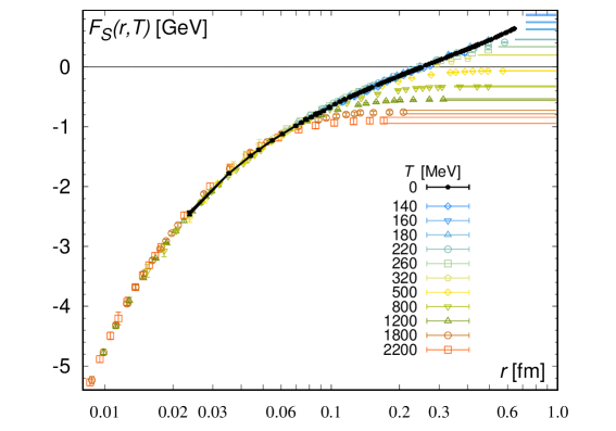
Our continuum results for are shown in Fig. 1 (left) and compared to the zero temperature static energy , shown as black pentagons connected by a thin black band. These represent the nonperturbatively improved static energy for five different lattice spacings in overlapping intervals. The details of the composition of these data are discussed in Appendix C. The numerical data for the zero temperature static energy are taken from Refs. Bazavov et al. (2012, 2014a, 2018). The asymptotic values, i.e., , are shown as horizontal bands. As one can see from the figure, at high temperatures, MeV, continuum results are available up to sufficiently large distances to see the approach to . At short distances, the singlet free energy is temperature independent and agrees with the vacuum static energy. At larger distances, we see the onset of medium effects. As the temperature is increased, the onset of the medium effects happens at shorter and shorter distances, but there is still an extended region in where agrees with the zero temperature static energy. This is expected from weak-coupling calculations in pNRQCD Berwein et al. (2017).
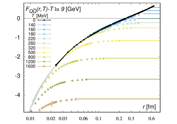
The continuum results for are shown in Fig. 1 (right). Again, only for MeV our continuum extrapolation extends to large enough distances to make connection to the asymptotic value of . To compare to the zero temperature static energy, we subtract the constant , which is due to the standard normalization convention of the Polyakov loop correlator defined by Eqs. (2) and (5), since usually the Polyakov loop correlator is defined without the normalization of the trace (see, e.g., Jahn and Philipsen (2004)). For the static energy, we use the same composite band as in the figure for . We extend this band to even shorter distances using the continuum limit of at very short distances as an estimate of . We show this estimate with a light gray color to keep the distinction clear and discuss the details of this band in Appendix C. For , we see a much larger temperature dependence already at relatively short distances and for temperatures MeV no clear agreement with the vacuum static energy can be seen. Qualitatively this behavior of the free energy and singlet free energy of is very similar to the results of previous calculations performed at fixed lattice spacing Karsch et al. (2001); Kaczmarek and Zantow (2005); Petreczky and Petrov (2004); Petreczky (2010); Bazavov and Petreczky (2013a); Borsanyi, Szabolcs and Fodor, Zoltan and Katz, Sándor D. and Pásztor, Attila and Szabó, Kálmán K. and Török, Csaba (2015). The reason for this behavior of the free energy is related to the presence of a color octet contribution and will be discussed in Sec. V. Finally, we mention that our continuum results for agree well with the continuum extrapolated results presented in Ref. Borsanyi, Szabolcs and Fodor, Zoltan and Katz, Sándor D. and Pásztor, Attila and Szabó, Kálmán K. and Török, Csaba (2015) for MeV. Our analysis, however, extends to higher temperatures.
III.3 The effective coupling
At it is customary to study the force between the static quark and antiquark defined in terms of the static energy or, equivalently, the corresponding effective coupling
| (15) |
where is the Casimir operator in the fundamental representation of SU(3). Following Ref. Kaczmarek et al. (2004) we can generalize this approach to the free energy and singlet free energy and obtain the corresponding effective couplings. The reasoning behind this generalization is that, as we see in Fig. 1, and are similar to at sufficiently small distances. At such distances, a sensible definition of an effective coupling seems possible.
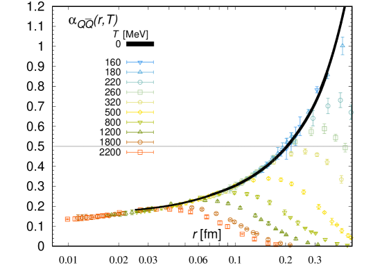
First, we discuss our numerical results for from the singlet free energy, which are shown in Fig. 2. The effective coupling defined in terms of is temperature independent at short distances and agrees with the result obtained from a numerical derivative of the static energy (details are given in Appendix C). At short distances, the running of the coupling is controlled by the scale . The effective coupling reaches a maximum at some distance and then decreases, indicating the onset of color screening. Furthermore, it turns out that approximately scales like . The distance roughly separates the region that is dominated by vacuum physics from the one where screening sets in.333 Note that screening starts affecting the effective coupling somewhat below . This will be addressed more quantitatively in the next section. It is interesting to see that the value of is quite large for MeV, implying that the physics is strongly coupled. At higher temperatures, , indicated by a horizontal line in the figure, so that weak-coupling methods might be applicable.
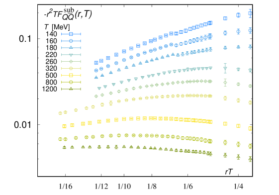
In the case of the free energy , we expect at short distances and for weak coupling two possible regimes. When , should exhibit a typical Coulombic behavior , whereas for , due to a cancellation between color singlet and color octet contributions, the behavior of as a function of the distance should be like . Indeed, the subtracted free energy, defined in Eq. (10), multiplied by , shown in Fig. 3,444 The apparent small discontinuities and pronounced variations of errors are an artifact of the analysis (cf. Sec. III.1). seems to exhibit both regimes. At short distances and for MeV, raises with the distance , a behavior consistent with , while for MeV, the available data for appear less sensitive to , a behavior consistent with . Analytical results and a detailed quantitative analysis can be found in Sec. V.1. Here our purpose is to justify the use of Eq. (15), at short distances and for MeV, to define an effective coupling also in the case of the free energy . Eventually, also this effective coupling can be compared with the coupling obtained from the static energy at zero temperature.
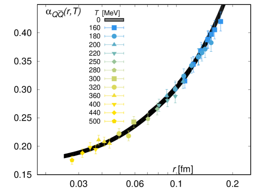
The statistical errors on our lattice results for are much larger than in the case and therefore we calculate the corresponding effective coupling only for finite . In Fig. 4, we show results for and . Following the above discussion, we look at temperatures MeV and at distances short enough that raises with the distance. Because of lack of accuracy of the derivative at the first data point for each temperature, we have to exclude derivatives for smaller than the center of the interval between the first two data points for each temperature. The points in Fig. 4 satisfy the above requirements. The figure supports a description where, in the considered temperature range and for the shortest distances, the free energy of a pair is dominated by the singlet contribution and agrees well with the static energy.
III.4 Cyclic Wilson loops
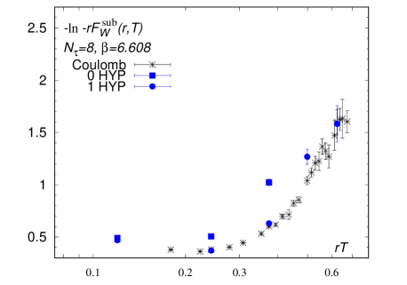
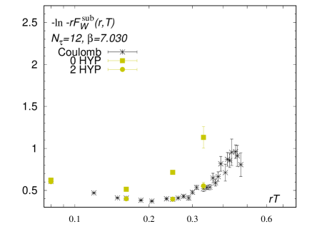
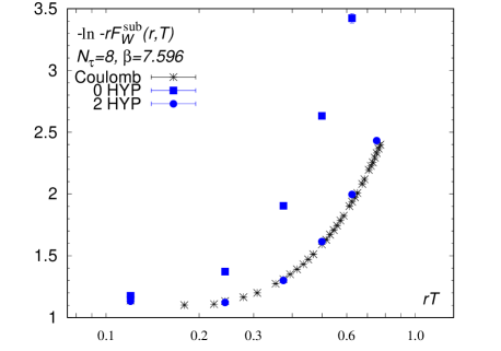
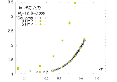
In this subsection, we present our numerical results for cyclic Wilson loops . Cyclic Wilson loops being gauge invariant offer an attractive possibility to study the medium modifications of interactions. From previous lattice results, we know that approaches at large distances Bazavov et al. (2009); Bazavov and Petreczky (2013c). This is also expected based on weak-coupling calculations Burnier et al. (2010). Like the Coulomb gauge singlet correlator, is also dominated by the singlet contribution at small distances Berwein et al. (2013, 2014). Moreover, weak-coupling calculations show that is screened at large distances like the Coulomb gauge singlet correlator. However, the study of cyclic Wilson loops is complicated by the presence of UV divergences. In the continuum theory, the renormalization of cyclic Wilson loops has been worked out for short distances, Berwein et al. (2013, 2014). However, on the lattice, we do not have enough data points at truly short distances to test these ideas. In part, this is due to the fact that off-axis separation cannot be used in the analysis (see the discussion in Sec. II). Therefore, we attempt to compare the unrenormalized smeared cyclic Wilson loops with the Coulomb gauge correlator. The smearing of the spatial links in is expected to reduce the size of UV divergences due to the self-energy, which are the largest divergences that affect the spatial lines. As we will see, for smeared cyclic Wilson loops, the UV divergences are sufficiently small at the considered values of to allow for a meaningful comparison.
We discuss our numerical results for cyclic Wilson loops in terms of . The analogy with Eq. (11) is obvious. We show the logarithm of in Fig. 5. There, we also show the usual Coulomb gauge singlet correlator in direct comparison. It is evident that from the unsmeared Wilson loop decays much more rapidly than the singlet correlator in the Coulomb gauge. This is due to the self-energy divergence of the spatial lines of the loop, which effectively increases the screening mass. As we increase the number of HYP smearing iterations, the size of the self-energy divergence in the spatial line is gradually reduced. After a few steps of HYP smearing, we obtain results for that agree with the results from the singlet correlator in the Coulomb gauge. The number of HYP smearing that is needed to sufficiently reduce the size of the self-energy divergence is larger for smaller lattice spacing. For higher temperatures, and thus finer lattice spacings at fixed , more smearing iterations are required in general, which can be seen by comparing the lower temperature (, upper panel in Fig. 5) with the higher temperature (, lower panel). We see that larger (finer lattices) requires larger numbers of smearing iterations to achieve a comparable effect. These findings are in qualitative agreement with the study performed in the SU(2) gauge theory Bazavov et al. (2008).
Though both correlators are affected by different technical difficulties, the accessible information regarding the interaction and the properties of the quark-gluon plasma seem to be similar.
IV Comparison of the singlet free energy to weak coupling
In this section, we compare the lattice results for the singlet free energy with the predictions of the weak-coupling calculations. These comparisons are the key for a deeper understanding of the mechanisms behind the onset of thermal effects with increasing separation of the pair and provide a tool to distinguish between electric and magnetic screening on the lattice.
The numerical results discussed in the previous section suggest that medium effects for the singlet free energy are small for . Furthermore, weak-coupling calculations have been worked out up to order for Berwein et al. (2017) and to next-to-leading order (NLO) for Burnier et al. (2010), which is accurate up to order Berwein et al. (2017). Hence, we will compare to the weak-coupling results separately for short () and large distances (). This separation of different regimes is, strictly speaking, valid only for asymptotically small couplings . However, as we will see below, the scale separation and the corresponding effective field theory calculations can also help to understand the lattice results when .
IV.1 Thermal corrections for small
Here we compare the lattice results with the weak-coupling calculations for . In this case the singlet free energy is given by the energy of a static pair in the vacuum , plus thermal corrections, which, however, are expected to be small. For this reason, it makes sense to perform the comparison with the lattice results in terms of the difference . The comparison of the lattice and weak-coupling results in terms of this difference has several advantages. First, one does not have to deal with the complications associated with the perturbative calculation of , among others, infrared logarithms (see Refs. Brambilla et al. (1999); Bazavov et al. (2014b)). Second, lattice artifacts largely cancel out in this difference, making the continuum extrapolations of this quantity simpler. Finally, the ultraviolet additive renormalization does not enter in .
We show our continuum results for in Fig. 6. The details of the continuum extrapolations are discussed in Appendix C. The difference in physical units is small at short distances and roughly temperature independent. As the temperature increases, the distances where medium effects are significant become smaller. Since we expect that thermal corrections should be proportional to the temperature, we present our results in temperature units in the right panel of Fig. 6. We see that for MeV the difference in temperature units approaches at short distances a constant. As we will explain in the next paragraph, this behavior is expected based on the weak-coupling calculations.
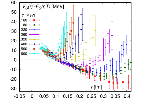
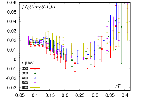
Now we discuss the comparison of with the weak-coupling calculations. From the point of view of weak-coupling calculations, short distances imply the scale hierarchy . In this regime, pNRQCD can be used. Moreover, the above scale hierarchy allows two further possible scale hierarchies: and . We discuss the second case, since here explicit calculations for are available up to unknown corrections of order and Berwein et al. (2017). The result reads
| (16) |
with contributions from the nonstatic gluons , from the quarks ( massless quark flavors) , and from the soft (Debye mass) scale ,
| (17) | ||||
| (18) | ||||
| (19) |
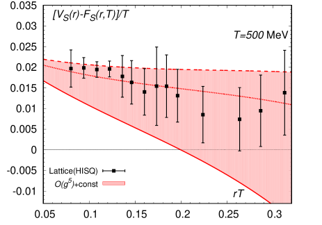
It is clear from the above expression that vanishes in the limit. This seems to be in apparent contradiction with the lattice results shown in Fig. 6. However, as remarked in Ref. Berwein et al. (2017) (see also the singlet normalization in Brambilla et al. (2000)), there is a possible order contribution, which is proportional to the temperature and independent of . Such a contribution would naturally explain the trend seen in the lattice results in Fig. 6 (right). Note that the term in Eq. (19) has the opposite sign with respect to the terms in Eqs. (17) and (18), leading to a partial cancellation. This partial cancellation is in fact responsible for relatively small medium effects in the considered distance region. In Fig. 7, we compare the lattice QCD results for to the perturbative calculation reproduced in Eq. (16). We use and the two-loop running coupling for this comparison. This choice of and running coupling gives , which is very close to the lattice QCD determination of based on the static energy Bazavov et al. (2014b), as well as to the lattice determination based on the charmonium correlators Maezawa and Petreczky (2016). For the renormalization scale, we choose and add a small constant to the above weak-coupling results, which mimics the possibly missing contribution such that the weak-coupling calculation agrees with the lattice at the shortest distance. We vary the renormalization scale by a factor of 2 around the central value to estimate the uncertainty of the perturbative result. This uncertainty is shown as a band in Fig. 7. Because of the partial cancellations between and , the net temperature shift of is relatively small for in agreement with the lattice results. Thus weak-coupling results obtained for enable us to explain the lattice findings on for small , i.e. for , in particular, their small temperature dependence. For larger distances, becomes numerically the dominant correction, even though it is parametrically small (order ) compared to and , which are of order . This means that screening effects become important, and the hierarchy of scales is not fulfilled anymore. We need to consider a weak-coupling expansion that does not assume such a hierarchy and resums screening effects right from the start. This is discussed in the next subsection.
There is no perturbative calculation of for the case . However, from the power counting, we expect thermal corrections to be small Brambilla et al. (2008). Furthermore, we also expect an -independent term proportional to appearing at order , since such a term possibly arises from the matching of pNRQCD to nonrelativistic QCD (NRQCD) Berwein et al. (2017). Therefore, several qualitative features of discussed above should also hold in this hierarchy of scales. This is quite different from the case of , where the two regimes and differ at leading order in the functional dependence on .
IV.2 Electric screening of the singlet free energy
In this subsection, we compare the lattice results for the singlet free energy with the weak-coupling prediction in the regime , i.e. in the electric screening regime. As mentioned in the Introduction, in this case EQCD can be used and the correlator can be calculated perturbatively. The physics in this regime is controlled to a large extent by the mass parameter of EQCD, , which is often called the Debye mass. At leading order
| (20) |
The comparison of the lattice and the weak-coupling results is performed in terms of the subtracted free energy defined in Eq. (11). The comparison in terms of is most convenient, since is very close to in this distance regime, and the weak-coupling calculations of are difficult Berwein et al. (2016, 2016). Our continuum results for are shown in Fig. 8. We clearly see that at decreases with increasing . This fact is consistent with the observation made in the previous section that medium effects become large at . The subtracted singlet free energy in the Coulomb gauge has been calculated at NLO in Ref. Burnier et al. (2010) using EQCD. We use Eq. (3.22) from that reference and omit the two-gluon exchange contribution proportional to , which is of order in the regime Berwein et al. (2017). The result reads
| (21) |
where is the exponential integral, i.e.
| (22) |
There are two corrections to the above result that are formally of higher order but numerically important. The first one is the correction due to the running coupling Burnier et al. (2010); Berwein et al. (2017), which can be written in the form Berwein et al. (2017)
| (23) |
with
| (24) |
The other correction is the correction to . The NLO result for the Debye mass, which has been calculated in Ref. Braaten and Nieto (1996), reads
| (25) |
In Fig. 8, we compare the weak-coupling results at LO and NLO with the continuum extrapolated lattice results. For the LO one, we use and for the NLO one, we use . For , we always use the above NLO result. As before, we use and the two-loop running coupling. We vary the scale from to to account for the uncertainty of the weak-coupling result. First of all, we see that the scale dependence is much reduced for higher temperatures. For MeV, it is sufficiently small to allow for an accurate comparison with the lattice. Moreover, the central value of the NLO result is always higher than the central value of the LO result. Within the uncertainty band, due to the variation of the scale, we see good agreement between the NLO result and the lattice data up to at least . For , the shape of the lattice results and the weak-coupling results is quite similar. At larger distances, however, the falloff of the lattice results is faster than the one of the NLO prediction. This is most likely due to the fact that, for these distances, the physics is affected by static chromomagnetic fields and, thus, it is nonperturbative. Based on previous calculations performed in the pure gauge theory, we expect that the effective screening mass governing the large distance behavior of the singlet correlator becomes significantly larger than due to chromomagnetic effects Heller et al. (1998); Karsch et al. (1998); Digal et al. (2003); Kaczmarek et al. (2004). This would explain the change in the slope at large distances that we observe. The behavior of in the large distance regime will be discussed in Sec. VI. However, it is important to stress that chromoelectric screening effects are important already at distances .
V Comparison of the Polyakov loop correlator to weak coupling
In this section, we compare the lattice results for the Polyakov loop correlator or, equivalently, the free energy of a static pair , with the predictions of the weak-coupling calculations. Here and in the following, we use small letters for the indices to mark color singlet or color octet objects defined in the framework of weak-coupling calculations and capital letters for the indices to mark color singlet or color octet objects defined in the context of nonperturbative lattice calculations. As in the case of the singlet free energy, we will perform this comparison separately for the short distance regime and for the screening regime, where .
V.1 The Polyakov loop correlator at short distances
We start by assuming the case . As it was discussed in Sec. III, the free energy of a static pair, , shows large deviations from the zero temperature static energy already at short distances. One way to understand this is in the language of pNRQCD. In the pNRQCD framework the Polyakov loop correlator at short distances can be written up to corrections of order as Berwein et al. (2017)
| (26) |
where and are gauge-invariant singlet and octet free energies defined in terms of pNRQCD correlators [see Eqs. (71) and (72) of Ref. Berwein et al. (2017)]. A good approximation of (26) is
| (27) |
where and are, respectively, the quark-antiquark color singlet and octet potentials at , and is the adjoint Polyakov loop expectation value. Equation (27) is valid up to corrections of order [cf. Eqs. (79) and (80) in Ref. Brambilla et al. (2010)]. From these equations, it is clear that the temperature dependence of the Polyakov loop correlator, and thus of the free energy comes, through the color octet contribution, mostly from .
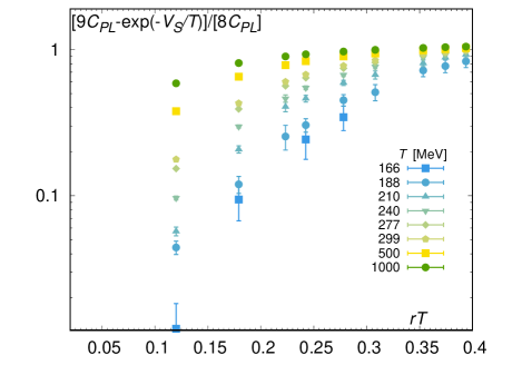
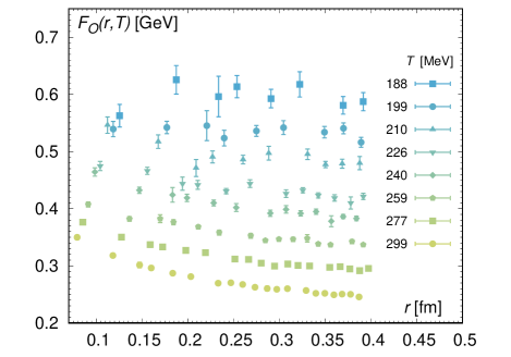
To test to what extent the above formulas work in the temperature and distance ranges considered in this study, we define the octet contribution to the Polyakov loop correlator as . In Fig. 9 (left panel) we show (normalized by ), which is a proxy for directly defined on the lattice. Specifically, this means that we are using lattice data for (on lattices) and the zero temperature static energy , calculated on the lattice in Refs. Bazavov et al. (2014a, 2018), as a proxy for . In this way, we avoid the complications associated with the perturbative calculation of . We see that increases with increasing temperatures and increasing distances. This can be understood by considering that is positive. Furthermore, at low temperatures, is small, thus leading to additional suppression of the octet contribution, while at high temperatures, is of order one Petreczky and Schadler (2015). According to Eq. (26), we can also parametrize as
| (28) |
Thus, the proxy defines a proxy for the octet free energy . The results for are also shown in Fig. 9 (right panel). We see that decreases with increasing temperatures. Moreover, for distances , we see hints for the presence of the repulsive tail .
To validate the pNRQCD framework on a quantitative level we reconstruct the subtracted free energy of a static pair using the pNRQCD decomposition formula (27) and lattice results for the zero temperature static energy , taken from Refs. Bazavov et al. (2014a, 2018), as a proxy for , and for the Polyakov loop expectation value in the fundamental representation, , taken from Ref. Bazavov et al. (2016). First, we write for the adjoint Polyakov loop,
| (29) |
where and are the Casimir operators of the fundamental and adjoint representations. The parameter is the measure of the breaking of Casimir scaling introduced in Ref. Petreczky and Schadler (2015). Casimir scaling implies and . It was found that is small above and compatible with zero for MeV Petreczky and Schadler (2015). Taking into account that and , we can then write for the subtracted energy
| (30) |
In the above equation, we have separated out the factor that breaks Casimir scaling for , which is the only purely perturbative input to Eq. (30). This correction was calculated in Ref. Kniehl et al. (2005),
| (31) |
Now, using the lattice results for and , we can calculate according to Eq. (30) and compare this to the results of direct lattice calculations of . This comparison is shown in Fig. 10 for at the two temperatures and MeV. The use of data for this comparison is justified because they are quite close to the continuum limit. As one can see from the figure, the pNRQCD decomposition formula works very well up to distances . For MeV, the octet contribution is very small and in fact can be omitted. For high temperatures, we could also use as a proxy for and obtain very similar results. We note that for high temperatures not only the octet contribution but also the breaking of Casimir scaling for in Eq. (31) is numerically important. If this breaking would be neglected, then the reconstruction of the Polyakov loop correlator in the right panel of Fig. 10 would only work for .
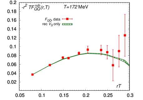
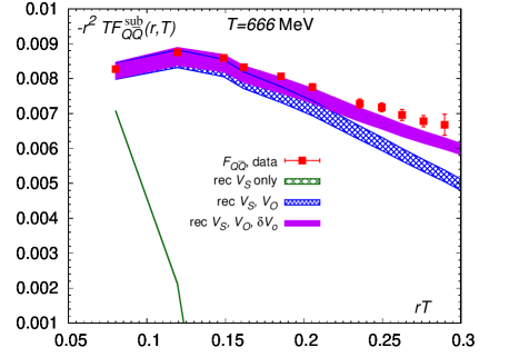
We have seen that pNRQCD can explain the lattice results for the Polyakov loop correlator at short distances. Up to distances of about , the behavior of the Polyakov loop correlator can be understood without invoking medium modification of the static quark-antiquark interactions [cf. Eq. (27)]. This is in agreement with our findings for the singlet free energy , which also shows that the interaction between the static quark and antiquark is only mildly affected by the medium up to distances .
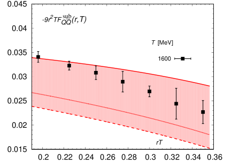
In order to compare the free energy with weak-coupling calculations, it is useful to distinguish two regimes. In the regime , we can expand the exponentials in the right-hand side of Eq. (26) and compute them in perturbation theory, obtaining at leading order in
| (32) |
which is valid up to corrections of order . Weak-coupling calculations have been performed in this case up to next-to-next-to-next-to-leading order (NNNLO), which is accurate up to order Berwein et al. (2017). In Fig. 11, we compare the NNNLO result for given by Eqs. (54) and (55) of Ref. Berwein et al. (2017) with the continuum extrapolated lattice result at MeV. We use three values of the renormalization scale: , , and . The running coupling has been calculated as before. We see that the lattice result and the weak-coupling result agree for , although the latter has a large uncertainty. At very small distances , the hierarchy breaks down.
In the regime , the right-hand side of Eq. (26) is dominated by the color singlet contribution. This happens at shorter and shorter distances as the temperature increases. We have seen in Fig. 3 that our lattice data appear to be sensitive to this regime so that we could even define an effective coupling and compare it in Fig. 4 with the strong coupling from the zero temperature force between a static pair.
V.2 The free energy in the screening regime
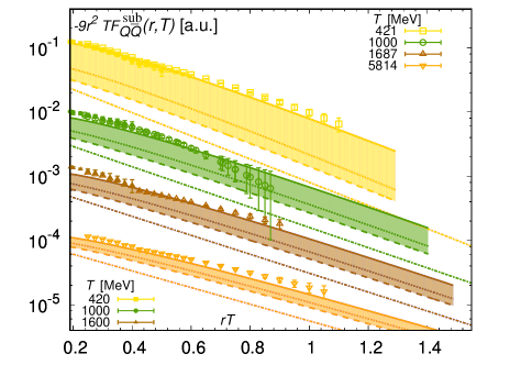
In the following, we study to which extent the weak-coupling expression for the free energy is able to describe the lattice data in the electric screening regime. In Sec. IV.2, we have shown that the singlet free energy is numerically consistent with the prediction of EQCD at NLO in the range . However, studies of the screening regime of the Polyakov loop correlator on the lattice are a daunting task. First, the signal-to-noise ratio of the Polyakov loop correlator is very poor, so we need very large statistics. Second, we find that, due to the smallness of the signal, finite volume effects in the subtracted free energy become important already for rather small separations. Hence we require lattices with large volumes. We satisfy these constraints by using the new ensembles with aspect ratio and total ensemble sizes of - gauge configurations. The smallness of the signal can be understood from the leading-order expression of the Polyakov loop correlator. Because of cancellations between singlet and octet contributions, mentioned in the previous subsection, the LO result for in the electric screening regime comes from the exchange of two electrostatic gluons Gross et al. (1981); McLerran and Svetitsky (1981); Nadkarni (1986),
| (33) |
Therefore, at large distances, is much smaller than .
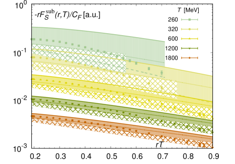
In Fig. 12, we show our results for the subtracted free energy as a function of at different temperatures. The numerical results for different temperatures have been shifted vertically for better visibility. The results at short distances, , and temperatures below have been extrapolated to the continuum limit (see Appendix C). The continuum extrapolated data are shown as filled symbols in Fig. 12. At large distances, the errors are large for and thus continuum extrapolations are not possible. To circumvent this problem, we correct the data for cutoff effects. We define the correction factor as the ratio between the continuum result for and the result: . Wherever the continuum result is available, the correction factor is known. Reliable continuum results are available only up to distances . We assume that at distances the correction factors are independent and equal to the correction factor at . Our analysis shows that cutoff effects are larger at larger distances (see Appendix C). As a consequence, the above procedure gives a continuum estimate that may be higher than the true continuum result (the continuum limit is approached from above). For the highest temperature considered in our study, namely, MeV, no continuum results are available. To make a continuum estimate at this temperature, we note that the correction factor decreases with increasing temperature because the cutoff effects become smaller at high temperatures (see Appendix C). The highest temperature where can be estimated is MeV. We assume that the cutoff effects at MeV are 2 times smaller than at MeV, i.e., we use .
Now let us compare the lattice results for with the weak-coupling calculations at , i.e. with the EQCD calculations. The free energy has been calculated at NLO in EQCD in Ref. Nadkarni (1986). Higher order corrections due to the running of the coupling are numerically important and have to be included in the analysis. These corrections have been computed in Ref. Berwein et al. (2017). Therefore, we use Eq. (64) of Ref. Berwein et al. (2017) , together with the NLO result for the Debye mass, Eq. (25), to obtain the weak-coupling result. Keeping only the first term in Eq. (64) of Ref. Berwein et al. (2017) corresponds to what we call the LO result, evaluated at the scale . As before, we use and the two-loop running coupling. The weak-coupling results are shown in Fig. 12. The dash-dotted lines correspond to the LO result for . The NLO results at different temperatures are shown as bands. We vary the scale from to to account for the scale uncertainty. The widths of the bands correspond to the scale uncertainties. We see again that the scale dependence reduces significantly at higher temperatures. The NLO result for is larger than the LO result and is significantly closer to the lattice data. Deviations between the lattice data and the NLO result for the scale are of the order of the statistical errors. Thus, for distances weak-coupling calculations in EQCD give a fair description of the lattice data, at least for the highest temperatures considered. In the next section, we will discuss the very large distance behavior of the static correlators, , where nonperturbative effects are important.
VI Asymptotic screening regime
In Secs. IV and V, we have shown that weak-coupling expansions describe lattice results fairly well both at short distances, , and at somewhat larger distances, , in the electric screening regime, where resummation is necessary. At distances much larger than the Debye length, , the magnetic screening, which is inherently nonperturbative, becomes important. Perturbative calculations are not valid in this regime. In this section, we discuss the behavior of the static quark correlators at large distances, i.e. . We expect that at these distances the correlators will be exponentially screened, i.e. behave like , with being a nonperturbative screening mass. As we will see, the challenge in the determination of the screening masses is the poor signal-to-noise ratio and possible contaminations from small distance physics.
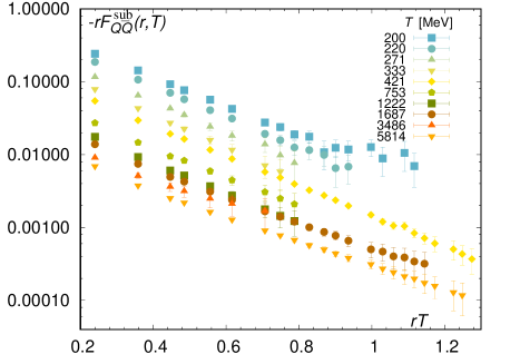
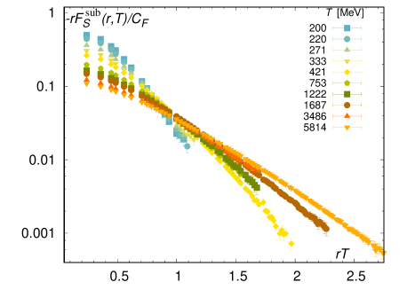
In Fig. 13 we show our numerical results for and multiplied by as function of on a logarithmic scale. At large values of , the above quantities should appear as straight lines in the figure. This is indeed the case, i.e. at sufficiently large distances, both and seem to decay exponentially. In the case of the singlet free energy, the data have some structure: the slope changes as we go from short to large distances. Furthermore, the slope increases with decreasing temperature, implying that the corresponding screening mass in temperature units increases at small temperatures. The fits of the correlators that we use for determining the screening masses clearly show this feature (see Appendix D). The lattice data for are relatively featureless. In particular, the slope seems independent of the temperature and the distance range considered. The data for also have much worse signal-to-noise ratio compared to the data for .
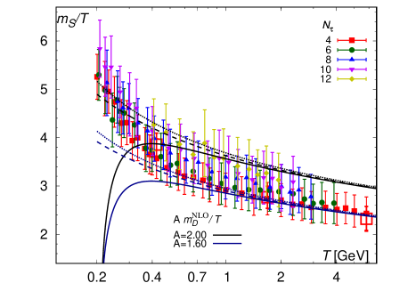
We discuss the details of the analysis of the asymptotic behavior and the extraction of the screening mass in Appendix D. We find that finite volume effects in the asymptotic behavior can be parametrized in terms of a constant shift between the correlators on lattices with different volumes (or aspect ratios ). After accounting for this constant shift, we find that screening masses are within errors independent of the volume for both and (see Appendix D).
We show the asymptotic screening mass from in Fig. 14 as a function of the temperature. The screening mass shows some cutoff dependence, which is only mildly temperature dependent. We do not see cutoff effects with a clear dependency on for , although screening masses with and appear to be systematically smaller. The screening mass is considerably larger than the perturbative Debye mass at NLO, Eq. (25). After we rescale by a constant -, we find that the temperature dependence of the screening mass and the rescaled Debye mass are very similar for high temperatures, . This rescaling factor is consistent with earlier observations in Refs. Kaczmarek et al. (2004); Kaczmarek (2007) using the LO Debye mass and much lower temperatures. A qualitatively similar enhancement was observed for the electric screening masses calculated from the Landau gauge gluon propagators Heller et al. (1998); Karsch et al. (1998). The two sets of lines in the figure represent the rescaled Debye mass with the scale varied from to .
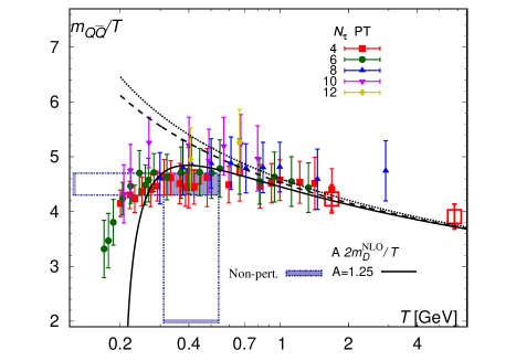
Because of the worse signal-to-noise ratio the fit of is more difficult. We have to restrict the fits to smaller range. This implies that the contamination from small distance physics could be potentially larger here. On the other hand, because the slope is independent of , we do not see a large sensitivity to the choice of the lower fit range. Our estimate of the corresponding screening mass is shown in Fig. 15. At high temperatures, this screening mass is clearly larger than the one extracted from . This is expected and is in agreement with previous findings. We compare our results with the screening mass determination on the lattice from EQCD Hart et al. (2000), which is shown as the horizontal band in Fig. 15. Our results and the EQCD result are in good agreement. At temperatures , the screening mass from the Polyakov loop correlator is only 25% larger than the naive perturbative result . This is consistent with the EQCD-based analysis Laine and Vepsalainen (2009). At temperatures around MeV, we see a decrease in . Such a decrease in the screening mass has been observed also in the SU(3) gauge theory Kaczmarek et al. (2000), where it is due to the (weakly) first-order nature of the deconfining transition and thus to the large correlation length of the order parameter (Polyakov loop).
The poor signal-to-noise ratio is clearly a problem for the determination of the screening masses. To overcome this problem, the Wilson lines should be evaluated on smeared gauge configurations before calculating the correlators, as in Ref. Borsanyi, Szabolcs and Fodor, Zoltan and Katz, Sándor D. and Pásztor, Attila and Szabó, Kálmán K. and Török, Csaba (2015). We plan to perform such a calculation in the future.
VII Conclusions
In this paper we have studied the free energy of a static pair and the static meson (singlet) correlator in (2+1)-flavor QCD with the aim to analyze at what distances the hot QCD medium modifies the interaction between the static quark and antiquark, and whether these modifications could be understood using perturbation theory. We have presented continuum extrapolated results for the free energy of a pair as well as for the singlet free energy in the Coulomb gauge.
At asymptotically high temperatures, , there are three distinct distance regimes: , , and . The physics in these regimes is quite different. In the first case, we expect only small thermal corrections to the quark-antiquark interaction. For , medium effects are significant and the interaction between the static quark and antiquark can be understood in terms of electric screening. At distances , nonperturbative effects due to static magnetic fields are important and the screening is nonperturbative.
Weak-coupling calculations of the Polyakov loop correlator and of the singlet correlator can be organized using effective field theories. For , one can use pNRQCD, while for , one can use EQCD. At larger distances, the screening masses have to be calculated nonperturbatively using lattice techniques Kajantie et al. (1997); Hart and Philipsen (2000); Hart et al. (2000).
For physically interesting temperatures the relevant coupling is . Thus, the question arises if the above picture and weak-coupling calculations are relevant at all. A related question is how well the different energy scales are separated and at what distances screening sets in. We have addressed these questions through a detailed comparison of lattice results with effective field-theory-based weak-coupling calculations. We have found that the weak-coupling picture provides a fair description for temperatures larger than MeV. For , medium effects are small, as predicted by pNRQCD. For , we see significant medium effects and the interaction between the static quark and antiquark is screened as predicted by perturbative EQCD. In this region, screening is controlled by the perturbative parameter . At larger separations, nonperturbative effects related to static chromomagnetic fields become important and the weak-coupling approach is no longer valid. In this region, we have determined the asymptotic screening masses by fitting the correlators at large distances.
The above results suggest that weak-coupling pNRQCD could be applicable for studying quarkonium properties at MeV. In a broader context, the success of the weak-coupling calculations for the Polyakov loop correlator and the singlet correlator is not completely surprising. Weak-coupling calculations have been found to agree well with lattice results for quark number susceptibilities Bazavov et al. (2013); Ding et al. (2015b); Bellwied et al. (2015), equation of state Borsanyi et al. (2016); Bazavov et al. (2018), and to some extent for the topological susceptibility (Borsanyi et al. (2016); Petreczky et al. (2016), see, however, Bonati et al. (2016)). Furthermore, the observed Casimir scaling of the Polyakov loop expectation values in higher representations Petreczky and Schadler (2015) is also naturally explained in the weak-coupling picture Berwein et al. (2016).
As a byproduct of this analysis, we have improved the accuracy of the renormalization constants of the Polyakov loop and the entropy of the single static quark (see Appendix A.3). We have also extended the study of cutoff effects for the static energy at short distances (see Appendix B). The latter may be of relevance for improved determinations of the strong coupling .
ACKNOWLEDGMENTS
This research was supported by the DFG cluster of excellence “Origin and Structure of the Universe” (www.universe-cluster.de). N. B., A. V. and J. H. W. acknowledge the support by the Bundesministerium für Bildung und Forschung (BMBF) under the Grant “Verbundprojekt 05P2015 - ALICE at High Rate (BMBF-FSP 202) GEM-TPC Upgrade and Field theory based investigations of ALICE physics,” Project No. 05P15WOCA1. This work has been supported in part by the U.S. Department of Energy through Award No. DE-SC0012704. The simulations have been carried out on the computing facilities of the National Energy Research Scientific Computing Center (NERSC), a U.S. Department of Energy Office of Science User Facility operated under Contract No. DE-AC02-05CH11231, the Computational Center for Particle and Astrophysics (C2PAP) as well as on the SuperMUC at the Leibniz- Rechenzentrum (LRZ). The lattice QCD calculations have been performed using the publicly available MILC code. The data analysis was performed using the R statistical package R Core Team (2018).
Appendix A GAUGE ENSEMBLES
In this Appendix, we give an account of the HISQ gauge ensembles underlying the presented lattice calculations. In Sec. A.1, we discuss the quark mass dependence in the new ensembles and finite volume effects. In Sec. A.2, we cover cuts in molecular dynamics (MD) trajectories due to thermalization, the determination of statistical errors, and the normalization using the MD time histories of the Polyakov loop. We discuss our cuts for the correlators. In Sec. A.3, we finally discuss the renormalization of and .
A.1 Lattices
| T (MeV) | : | #TUs | Ref. | ||
|---|---|---|---|---|---|
| 6.515 | 0.0604 | 122 | 0.21, 0.15 | 32500 | Bazavov et al. (2016) |
| 6.608 | 0.0542 | 133 | 0.26, 0.18 | 19990 | Bazavov et al. (2016) |
| 6.664 | 0.0514 | 141 | 0.26, 0.24 | 45120 | Bazavov et al. (2016) |
| 6.700 | 0.0496 | 146 | 0.21, 0.21 | 15900 | Bazavov et al. (2016) |
| 6.740 | 0.0476 | 151 | 0.31, 0.24 | 29410 | Bazavov et al. (2014a) |
| 6.770 | 0.0460 | 156 | 0.31, 0.21 | 15530 | Bazavov et al. (2016) |
| 6.800 | 0.0448 | 160 | 0.34, 0.26 | 36060 | Bazavov et al. (2014a) |
| 6.840 | 0.0430 | 166 | 0.35, 0.24 | 17370 | Bazavov et al. (2016) |
| 6.880 | 0.0412 | 173 | 0.37, 0.28 | 46350 | Bazavov et al. (2014a) |
| 6.950 | 0.0386 | 185 | 0.39, 0.30 | 50550 | Bazavov et al. (2016) |
| 7.030 | 0.0378 | 199 | 0.47, 0.39 | 65940 | Bazavov et al. (2014a) |
| 7.100 | 0.0332 | 213 | 0.46, 0.30 | 9640 | Bazavov et al. (2013) |
| 7.150 | 0.0320 | 223 | 0.45, 0.35 | 9600 | Bazavov et al. (2014a) |
| 7.200 | 0.0296 | 233 | 0.38, 0.31 | 4010 | Bazavov et al. (2013) |
| 7.280 | 0.0284 | 251 | 0.55, 0.47 | 58210 | Bazavov et al. (2014a) |
| 7.373 | 0.0250 | 273 | 0.57, 0.55 | 85120 | Bazavov et al. (2014a) |
| 7.596 | 0.0202 | 334 | 0.72, 0.57 | 98010 | Bazavov et al. (2014a) |
| 7.650 | 0.0202 | 350 | 0.54, 0.39 | 3230 | Bazavov et al. (2013) |
| 7.825 | 0.0164 | 408 | 0.94, 0.60 | 134600 | Bazavov et al. (2014a) |
| 8.000 | 0.0140 | 474 | 0.68, 0.54 | 3110 | Ding et al. (2015a) |
| 8.200 | 0.01167 | 562 | 1.05, 0.76 | 30090 | Ding et al. (2015a) |
| 8.400 | 0.00975 | 667 | 1.06, 0.72 | 29190 | Ding et al. (2015a) |
| T (MeV) | : | #TUs | Ref. | ||
|---|---|---|---|---|---|
| 6.285 | 0.0790 | 116 | 0.22, 0.18 | 9260 | Bazavov et al. (2016) |
| 6.341 | 0.0740 | 123 | 0.25, 0.22 | 39190 | Bazavov et al. (2016) |
| 6.423 | 0.0670 | 133 | 0.25, 0.19 | 10360 | Bazavov et al. (2016) |
| 6.488 | 0.0620 | 142 | 0.37, 0.30 | 102690 | Bazavov et al. (2014a) |
| 6.515 | 0.0604 | 146 | 0.37, 0.33 | 107530 | Bazavov et al. (2014a) |
| 6.575 | 0.0564 | 155 | 0.37, 0.33 | 106020 | Bazavov et al. (2014a) |
| 6.608 | 0.0542 | 160 | 0.46, 0.33 | 112890 | Bazavov et al. (2014a) |
| 6.664 | 0.0514 | 169 | 0.51, 0.46 | 155440 | Bazavov et al. (2014a) |
| 6.740 | 0.0476 | 181 | 0.57, 0.55 | 200250 | Bazavov et al. (2014a) |
| 6.800 | 0.0448 | 192 | 0.55, 0.61 | 279830 | Bazavov et al. (2014a) |
| 6.880 | 0.0412 | 208 | 0.66, 0.68 | 341490 | Bazavov et al. (2014a) |
| 6.950 | 0.0386 | 222 | 0.68, 0.73 | 243480 | Bazavov et al. (2014a) |
| 7.030 | 0.0378 | 239 | 0.68, 0.68 | 137730 | Bazavov et al. (2014a) |
| 7.150 | 0.0320 | 267 | 0.79, 0.76 | 145440 | Bazavov et al. (2014a) |
| 7.280 | 0.0284 | 301 | 0.93, 0.71 | 105990 | Bazavov et al. (2014a) |
| 7.373 | 0.0250 | 328 | 0.97, 0.68 | 50840 | Bazavov et al. (2014a) |
| 7.596 | 0.0202 | 400 | 1.09, 0.81 | 51710 | Bazavov et al. (2014a) |
| 7.825 | 0.0164 | 489 | 1.15, 0.83 | 54000 | Bazavov et al. (2014a) |
| 8.000 | 0.0140 | 569 | 1.09, 1.00 | 6780 | Ding et al. (2015a) |
| 8.200 | 0.01167 | 675 | 1.12, 0.57 | 27500 | Ding et al. (2015a) |
| 8.400 | 0.00975 | 800 | 1.07, 0.58 | 7540 | Ding et al. (2015a) |
| 8.570 | 0.008376 | 924 | 1.31, 0.93 | 3000 | Bazavov et al. (2013) |
| T (MeV) | : | #TUs | Ref. | ||
|---|---|---|---|---|---|
| 6.050 | 0.1064 | 116 | 0.31, 0.35 | 47130 | Bazavov et al. (2014a) |
| 6.125 | 0.0966 | 125 | 0.31, 0.31 | 8980 | Bazavov et al. (2014a) |
| 6.175 | 0.0906 | 131 | 0.28, 0.22 | 1520 | Bazavov et al. (2014a) |
| 6.195 | 0.0880 | 133 | 0.39, 0.35 | 16900 | Bazavov et al. (2014a) |
| 6.245 | 0.0830 | 140 | 0.41, 0.31 | 26100 | Bazavov et al. (2014a) |
| 6.260 | 0.0810 | 142 | 0.39, 0.35 | 10240 | Bazavov et al. (2014a) |
| 6.285 | 0.0790 | 146 | 0.41, 0.37 | 31440 | Bazavov et al. (2014a) |
| 6.315 | 0.0760 | 150 | 0.45, 0.35 | 7850 | Bazavov et al. (2014a) |
| 6.341 | 0.0740 | 154 | 0.41, 0.45 | 17130 | Bazavov et al. (2014a) |
| 6.354 | 0.0728 | 156 | 0.41, 0.47 | 12540 | Bazavov et al. (2014a) |
| 6.390 | 0.0694 | 161 | 0.47, 0.43 | 26950 | Bazavov et al. (2014a) |
| 6.423 | 0.0670 | 167 | 0.52, 0.53 | 20310 | Bazavov et al. (2014a) |
| 6.445 | 0.0652 | 170 | 0.53, 0.55 | 13630 | Bazavov et al. (2014a) |
| 6.460 | 0.0640 | 173 | 0.53, 0.43 | 16430 | Bazavov et al. (2014a) |
| 6.488 | 0.0620 | 178 | 0.56, 0.55 | 17900 | Bazavov et al. (2014a) |
| 6.515 | 0.0604 | 182 | 0.56, 0.56 | 24800 | Bazavov et al. (2014a) |
| 6.550 | 0.0682 | 189 | 0.59, 0.47 | 23560 | Bazavov et al. (2014a) |
| 6.575 | 0.0564 | 193 | 0.64, 0.65 | 26300 | Bazavov et al. (2014a) |
| 6.608 | 0.0542 | 200 | 0.69, 0.69 | 24190 | Bazavov et al. (2014a) |
| 6.664 | 0.0514 | 211 | 0.69, 0.72 | 19000 | Bazavov et al. (2014a) |
| 6.740 | 0.0476 | 227 | 0.69, 0.72 | 20160 | Bazavov et al. (2014a) |
| 6.800 | 0.0448 | 240 | 0.80, 0.80 | 16760 | Bazavov et al. (2014a) |
| 6.880 | 0.0412 | 259 | 0.84, 0.75 | 27400 | Bazavov et al. (2014a) |
| 6.950 | 0.0386 | 277 | 0.85, 0.71 | 24700 | Bazavov et al. (2014a) |
| 7.030 | 0.0378 | 299 | 0.94, 0.83 | 25570 | Bazavov et al. (2014a) |
| 7.150 | 0.0320 | 334 | 0.85, 0.65 | 19340 | Bazavov et al. (2014a) |
| 7.280 | 0.0284 | 377 | 1.08, 0.81 | 31990 | Bazavov et al. (2014a) |
| 7.373 | 0.0250 | 410 | 1.19, 0.96 | 119380 | Bazavov et al. (2014a) |
| 7.500 | 0.0222 | 459 | 0.82, 0.50 | 4990 | Bazavov et al. (2013) |
| 7.596 | 0.0202 | 500 | 1.29, 0.85 | 127990 | Bazavov et al. (2014a) |
| 7.825 | 0.0164 | 611 | 1.31, 0.83 | 122200 | Bazavov et al. (2014a) |
| 8.000 | 0.0140 | 711 | 1.27, 0.75 | 18370 | Bazavov et al. (2013) |
| 8.200 | 0.01167 | 843 | 1.10, 0.52 | 3080 | Bazavov et al. (2013) |
| 8.400 | 0.00975 | 1000 | 1.14, 0.69 | 3000 | Bazavov et al. (2013) |
| 8.570 | 0.008376 | 1155 | 1.16, 0.69 | 10250 | Bazavov et al. (2016) |
| 8.710 | 0.007394 | 1299 | 1.21, 0.72 | 10030 | Bazavov et al. (2016) |
| 8.850 | 0.006528 | 1461 | 1.48, 0.84 | 10000 | Bazavov et al. (2016) |
| 9.060 | 0.004834 | 1743 | 1.29, 0.62 | 10810 | Bazavov et al. (2016) |
| 9.230 | 0.004148 | 2011 | 1.29, 0.67 | 10250 | Bazavov et al. (2016) |
| 9.360 | 0.003691 | 2242 | 1.47, 0.64 | 8120 | Bazavov et al. (2016) |
| 9.490 | 0.003285 | 2500 | 1.51, 0.71 | 8010 | Bazavov et al. (2016) |
| 9.670 | 0.002798 | 2907 | 1.58, 0.67 | 8050 | Bazavov et al. (2016) |
| T (MeV) | : | #TUs | Ref. | ||
|---|---|---|---|---|---|
| 5.900 | 0.1320 | 134 | 0.47, 0.47 | 31070 | Bazavov et al. (2014a) |
| 6.000 | 0.1138 | 147 | 0.55, 0.58 | 31640 | Bazavov et al. (2014a) |
| 6.050 | 0.1064 | 154 | 0.53, 0.55 | 29990 | Bazavov et al. (2014a) |
| 6.100 | 0.0998 | 162 | 0.62, 0.69 | 29990 | Bazavov et al. (2014a) |
| 6.150 | 0.0936 | 170 | 0.55, 0.76 | 27990 | Bazavov et al. (2014a) |
| 6.195 | 0.0880 | 178 | 0.69, 0.78 | 29990 | Bazavov et al. (2014a) |
| 6.215 | 0.0862 | 181 | 0.55, 0.74 | 5390 | Bazavov et al. (2014a) |
| 6.245 | 0.0830 | 187 | 0.76, 0.83 | 30000 | Bazavov et al. (2014a) |
| 6.285 | 0.0790 | 194 | 0.55, 0.60 | 5750 | Bazavov et al. (2014a) |
| 6.341 | 0.0740 | 205 | 0.76, 0.90 | 30000 | Bazavov et al. (2014a) |
| 6.423 | 0.0670 | 222 | 0.90, 0.87 | 29990 | Bazavov et al. (2014a) |
| 6.515 | 0.0604 | 243 | 0.91, 0.94 | 29990 | Bazavov et al. (2014a) |
| 6.575 | 0.0564 | 258 | 1.01, 0.91 | 29990 | Bazavov et al. (2014a) |
| 6.608 | 0.0542 | 266 | 1.03, 0.91 | 29990 | Bazavov et al. (2014a) |
| 6.664 | 0.0514 | 281 | 1.01, 0.78 | 29990 | Bazavov et al. (2014a) |
| 6.800 | 0.0448 | 320 | 1.07, 0.91 | 29990 | Bazavov et al. (2014a) |
| 6.950 | 0.0386 | 370 | 1.13, 0.90 | 29990 | Bazavov et al. (2014a) |
| 7.150 | 0.0320 | 446 | 1.30, 0.97 | 25500 | Bazavov et al. (2014a) |
| 7.280 | 0.0284 | 502 | 1.25, 0.83 | 27140 | Bazavov et al. (2014a) |
| 7.373 | 0.0250 | 547 | 1.25, 0.78 | 24120 | Bazavov et al. (2014a) |
| 7.500 | 0.0222 | 613 | 1.35, 0.91 | 5670 | Bazavov et al. (2013) |
| 7.596 | 0.0202 | 667 | 1.35, 0.78 | 33520 | Bazavov et al. (2014a) |
| 7.825 | 0.0164 | 815 | 1.67, 1.00 | 30440 | Bazavov et al. (2014a) |
| 8.000 | 0.0140 | 948 | 1.39, 0.85 | 3200 | Bazavov et al. (2013) |
| 8.200 | 0.01167 | 1125 | 1.30, 0.76 | 10100 | Bazavov et al. (2016) |
| 8.400 | 0.00975 | 1334 | 1.31, 0.82 | 10160 | Bazavov et al. (2016) |
| 8.570 | 0.008376 | 1540 | 1.39, 0.71 | 10190 | Bazavov et al. (2016) |
| 8.710 | 0.007394 | 1732 | 1.39, 0.96 | 10220 | Bazavov et al. (2016) |
| 8.850 | 0.006528 | 1949 | 1.36, 0.74 | 10060 | Bazavov et al. (2016) |
| 9.060 | 0.004834 | 2324 | 1.52, 0.96 | 10070 | Bazavov et al. (2016) |
| 9.230 | 0.004148 | 2681 | 1.43, 0.85 | 10060 | Bazavov et al. (2016) |
| 9.360 | 0.003691 | 2989 | 1.64, 0.90 | 8240 | Bazavov et al. (2016) |
| 9.490 | 0.003285 | 3333 | 1.55, 0.62 | 8130 | Bazavov et al. (2016) |
| 9.670 | 0.002798 | 3876 | 1.41, 0.62 | 10290 | Bazavov et al. (2016) |
| T (MeV) | : | #TUs | Ref. | ||
|---|---|---|---|---|---|
| 5.900 | 0.132000 | 201 | 0.90, 1.17 | 65350 | Bazavov et al. (2016) |
| 6.000 | 0.113800 | 221 | 1.09, 1.06 | 62610 | Bazavov et al. (2016) |
| 6.050 | 0.106400 | 232 | 1.12, 1.12 | 62400 | Bazavov et al. (2016) |
| 6.125 | 0.096600 | 249 | 1.14, 1.06 | 63510 | Bazavov et al. (2016) |
| 6.215 | 0.086200 | 272 | 1.06, 0.94 | 26650 | Bazavov et al. (2016) |
| 6.285 | 0.079000 | 291 | 1.14, 1.00 | 25380 | Bazavov et al. (2016) |
| 6.354 | 0.072800 | 311 | 1.12, 0.94 | 19480 | Bazavov et al. (2016) |
| 6.423 | 0.067000 | 333 | 1.14, 0.87 | 21930 | Bazavov et al. (2016) |
| 6.515 | 0.060300 | 364 | 1.14, 0.90 | 31330 | Bazavov et al. (2016) |
| 6.575 | 0.056400 | 386 | 1.22, 0.87 | 22770 | Bazavov et al. (2016) |
| 6.608 | 0.054200 | 399 | 1.30, 1.09 | 39400 | Bazavov et al. (2016) |
| 6.664 | 0.051400 | 421 | 1.46, 1.22 | 75770 | Bazavov et al. (2016) |
| 6.800 | 0.044800 | 480 | 1.14, 0.71 | 37860 | Bazavov et al. (2016) |
| 6.950 | 0.038600 | 554 | 1.22, 0.79 | 38090 | Bazavov et al. (2016) |
| 7.150 | 0.032000 | 669 | 1.25, 0.62 | 31800 | Bazavov et al. (2016) |
| 7.280 | 0.028400 | 753 | 1.30, 0.87 | 42810 | Bazavov et al. (2016) |
| 7.373 | 0.025000 | 819 | 1.62, 1.00 | 65010 | Bazavov et al. (2016) |
| 7.500 | 0.022200 | 918 | 1.60, 0.87 | 42950 | Bazavov et al. (2016) |
| 7.596 | 0.020200 | 1000 | 1.54, 0.83 | 69920 | Bazavov et al. (2016) |
| 7.825 | 0.016400 | 1222 | 1.68, 0.90 | 65380 | Bazavov et al. (2016) |
| 8.000 | 0.014000 | 1422 | 1.52, 0.71 | 27510 | Bazavov et al. (2016) |
| 8.200 | 0.011670 | 1687 | 1.54, 0.87 | 20790 | Bazavov et al. (2016) |
| 8.400 | 0.009750 | 1999 | 1.48, 0.71 | 20950 | Bazavov et al. (2016) |
| 8.570 | 0.008376 | 2308 | 1.68, 0.90 | 20280 | Bazavov et al. (2016) |
| 8.710 | 0.007394 | 2597 | 1.60, 0.71 | 20200 | Bazavov et al. (2016) |
| 8.850 | 0.006528 | 2921 | 1.52, 0.71 | 19210 | Bazavov et al. (2016) |
| 9.060 | 0.004834 | 3487 | 1.66, 1.00 | 20950 | Bazavov et al. (2016) |
| 9.230 | 0.004148 | 4021 | 1.70, 0.87 | 21240 | Bazavov et al. (2016) |
| 9.360 | 0.003691 | 4484 | 1.44, 0.56 | 10620 | Bazavov et al. (2016) |
| 9.490 | 0.003285 | 5000 | 1.62, 0.79 | 10320 | Bazavov et al. (2016) |
| 9.670 | 0.002798 | 5814 | 1.64, 0.87 | 10340 | Bazavov et al. (2016) |
| : | ||||||
| T (MeV) | , | : | #TUs | |||
| 8.570 | 0.008376 | 770 | 48, 48 | 1.03, 0.49 | 6320 | 0.033869(75) |
| 8.710 | 0.007394 | 866 | 48, 48 | 1.06, 0.55 | 6490 | 0.037745(84) |
| 8.850 | 0.006528 | 974 | 48, 48 | 1.09, 0.58 | 6340 | 0.41749(101) |
| 9.060 | 0.004834 | 1162 | 48, 96 | 1.15, 0.60 | 7430 | 0.048343(66) |
| 9.230 | 0.004148 | 1340 | 48, 48 | 1.17, 0.53 | 7280 | 0.053533(85) |
| 9.360 | 0.003691 | 1495 | 48, 96 | 1.25, 0.62 | 7910 | 0.057509(70) |
| 9.490 | 0.003285 | 1667 | 48, 48 | 1.15, 0.53 | 9780 | 0.061575(63) |
| 9.670 | 0.002798 | 1938 | 48, 96 | 1.25, 0.72 | 7650 | 0.067389(55) |
| : | ||||||
| T (MeV) | , | : | #TUs | |||
| 8.710 | 0.007394 | 1039 | 40, 40 | 1.17, 0.59 | 15320 | 0.068687(92) |
| 8.850 | 0.006528 | 1169 | 40, 80 | 1.28, 0.87 | 7690 | 0.074258(86) |
| 9.060 | 0.004834 | 1395 | 40, 40 | 1.31, 0.64 | 15490 | 0.083071(70) |
| 9.230 | 0.004148 | 1608 | 40, 80 | 1.39, 0.60 | 7630 | 0.090309(95) |
| 9.360 | 0.003691 | 1794 | 40, 40 | 1.30, 0.61 | 15800 | 0.095748(78) |
| 9.490 | 0.003285 | 2000 | 40, 80 | 1.26, 0.62 | 7990 | 0.101253(107) |
| 9.670 | 0.002798 | 2326 | 40, 40 | 1.38, 0.74 | 15760 | 0.108795(110) |
| : | ||||||
|---|---|---|---|---|---|---|
| T (MeV) | : | #TUs | ||||
| 7.825 | 0.00164 | 306 | 1/20 | 0.39, 0.31 | 10780 | 0.002975(14) |
| 8.000 | 0.001299 | 356 | 1/5 | 0.42, 0.29 | 11460 | 0.004185(17) |
| 8.200 | 0.001071 | 422 | 1/5 | 0.42, 0.29 | 10660 | 0.005908(18) |
| 8.400 | 0.000887 | 500 | 1/5 | 0.60, 0.34 | 11410 | 0.007813(26) |
| 8.570 | 0.008376 | 577 | 1/20 | 0.61, 0.36 | 10400 | 0.009680(28) |
| 8.710 | 0.007394 | 650 | 1/20 | 0.65, 0.40 | 10190 | 0.0113707(21) |
| 8.850 | 0.006528 | 731 | 1/20 | 0.67, 0.42 | 4480 | 0.013246(32) |
| 9.060 | 0.004834 | 872 | 1/20 | 0.82, 0.42 | 8350 | 0.015904(33) |
| 9.230 | 0.004148 | 1005 | 1/20 | 0.76, 0.99 | 3610 | 0.018594(62) |
| 9.360 | 0.003691 | 1121 | 1/20 | 0.82, 0.34 | 3530 | 0.020562(52) |
| 9.490 | 0.003285 | 1250 | 1/20 | 0.86, 0.36 | 6790 | 0.022477(46) |
| 9.670 | 0.002798 | 1454 | 1/20 | 0.86, 0.76 | 8320 | 0.025508(52) |
| : | |||||||||
| T (MeV) | : | #TUs | : | #TUs | |||||
| 8.000 | 474 | 0.01400 | 0.68, 0.54 | 3110 | 0.019196(90) | 0.01299 | 1.06, 0.77 | 71670 | 0.019254(25) |
| 8.200 | 563 | 0.01167 | 1.05, 0.76 | 30090 | 0.024060(43) | 0.01071 | 1.09, 0.73 | 71390 | 0.024062(25) |
| 8.400 | 667 | 0.00975 | 1.06, 0.72 | 29190 | 0.029300(41) | 0.00887 | 1.15, 0.70 | 71170 | 0.029252(24) |
| : | |||||||||
| T (MeV) | : | #TUs | : | #TUs | |||||
| 8.000 | 569 | 0.01400 | 1.09, 1.00 | 6780 | 0.040275(211) | 0.01299 | 1.21, 0.80 | 82770 | 0.040215(36) |
| 8.200 | 675 | 0.01167 | 1.12, 0.57 | 27500 | 0.047833(97) | 0.01071 | 1.31, 0.83 | 72180 | 0.048010(33) |
| 8.400 | 800 | 0.00975 | 1.07, 0.58 | 7540 | 0.055774(114) | 0.00887 | 1.27, 0.83 | 72770 | 0.055918(38) |
| : | |||||||||
| T (MeV) | : | #TUs | : | #TUs | |||||
| 7.825 | 611 | 0.0164 | 1.31, 0.83 | 122200 | 0.072566(29) | 0.01542 | 1.36, 0.91 | 51510 | 0.072616(44) |
| 8.000 | 711 | 0.01400 | 1.27, 0.75 | 18370 | 0.083107(317) | 0.01299 | 1.53, 0.95 | 100770 | 0.082665(32) |
| 8.200 | 843 | 0.01167 | 1.10, 0.52 | 3080 | 0.093920(224) | 0.01071 | 1.59, 1.08 | 100410 | 0.094084(41) |
| 8.400 | 1000 | 0.00975 | 1.14, 0.69 | 3000 | 0.105302(286) | 0.00887 | 1.49, 0.91 | 100830 | 0.105537(48) |
| : | |||||||||
| T (MeV) | : | #TUs | : | #TUs | |||||
| 7.030 | 399 | 0.0356 | 1.25, 0.96 | 30390 | 0.083622(82) | 0.0356 | 1.13, 0.83 | 30830 | 0.083627(91) |
| 7.825 | 824 | 0.0164 | 1.67, 1.00 | 54480 | 0.151915(64) | 0.01542 | 1.34, 0.78 | 59450 | 0.151974(63) |
| 8.000 | 948 | 0.01400 | 1.39, 0.85 | 3200 | 0.165828(296) | 0.01299 | 1.56, 0.94 | 102210 | 0.165650(53) |
| 8.200 | 1125 | 0.01167 | 1.30, 0.76 | 10100 | 0.180802(171) | 0.01071 | 1.74, 1.09 | 102360 | 0.181024(57) |
| 8.400 | 1334 | 0.00975 | 1.31, 0.82 | 10160 | 0.195736(153) | 0.00887 | 1.80, 1.13 | 102700 | 0.195837(50) |
| : | |||||||||
| T (MeV) | : | #TUs | : | #TUs | |||||
| 7.030 | 598 | 0.0356 | 1.58, 1.03 | 52640 | 0.229883(83) | 0.0356 | 1.46, 0.90 | 50230 | 0.229996(76) |
| 7.825 | 1222 | 0.0164 | 1.68, 0.90 | 65380 | 0.315334(66) | 0.01542 | 1.70, 1.03 | 50390 | 0.315231(93) |
| 8.000 | 1422 | 0.01400 | 1.52, 0.71 | 27510 | 0.331131(96)) | 0.01299 | 1.60, 0.94 | 97570 | 0.331104(44) |
| 8.200 | 1687 | 0.01167 | 1.54, 0.87 | 20790 | 0.348063(122) | 0.01071 | 1.87, 1.03 | 99810 | 0.348141(59) |
| 8.400 | 1999 | 0.00975 | 1.48, 0.71 | 20950 | 0.363987(151) | 0.00887 | 1.62, 0.90 | 100000 | 0.364152(46) |
| : | ||||||||
|---|---|---|---|---|---|---|---|---|
| T (MeV) | : | #TUs | : | #TUs | ||||
| 6.664 | 421 | 0.0514 | 1.46, 1.22 | 75770 | 0.180018(82) | 1.92, 1.27 | 513260 | 0.180141(15) |
| 8.200 | 1687 | 0.01071 | 1.87, 1.03 | 99810 | 0.348141(59) | 2.26, 1.27 | 203980 | 0.348081(16) |
| 9.670 | 5814 | 0.002798 | 1.64, 0.87 | 10340 | 0.447998(137) | 2.77, 1.37 | 600760 | 0.448130(11) |
As mentioned in Sec. II, we make use of gauge ensembles from the HotQCD Collaboration and from an earlier publication of the TUMQCD Collaboration (cf. Refs. Bazavov et al. (2012, 2014a); Ding et al. (2015b); Bazavov et al. (2013); Bazavov and Petreczky (2013b); Bazavov et al. (2016)). The parameters of these gauge configurations, the collected statistics that have been used for the correlators in this study, as well as references to the original publications are listed in Tables 1 – 5. These lattices have light sea quark masses of and correspond to a pion mass of in the continuum limit. Temperatures in the tables have been fixed using the scale. Most ensembles are available in the form of multiple streams of molecular dynamics (MD) time evolution with different starting lattices and different seeds of the pseudorandom number generator. The different streams of each ensemble are indexed by single letters in alphabetical ordering, i.e. the first stream is the “a” stream. Although all streams have roughly similar length for most ensembles, there are cases where additional streams have been branched off the first streams much later and are therefore substantially shorter. The first 30 time units (TUs) of each stream of HotQCD lattices (40 TUs for TUMQCD lattices) use the rational hybrid molecular dynamics (RHMD) algorithm instead of the rational hybrid Monte Carlo (RHMC) algorithm Clark et al. (2005). This approach avoids small acceptance rates due to large changes of the action during early thermalization and shortens the thermalization phase to typically 20-40 TUs. To be safe, we later omit at least 100 TUs of the initial lattices of each stream in the analysis. For an unclear reason, we found a problem with thermalization of the gauge ensemble. We generated a new ensemble with the same parameters from scratch, which we use in our analysis (cf. Table 8). In order to take the continuum limit for extremely high temperatures, , we generated new very fine ensembles with and (cf. Table 6). In order to ensure control of cutoff effects at the smallest separations, we generated another set of gauge ensembles with (cf. Table 7).
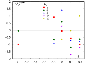
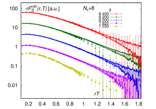
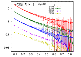
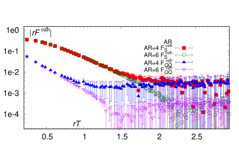
Furthermore, we generated new lattices with a larger light sea quark mass, corresponding to a pion mass of in the continuum limit. These new lattices have and and , and and therefore span a temperature range from to . Since these lattices have high temperatures (), numerical results are only mildly affected by the larger quark mass. We summarize these ensembles in Table 8. In the left panel of Fig. 16, we show a ratio of the difference between the bare single quark free energies with different light sea quark masses and over the combined uncertainty, obtained by adding their statistical errors in quadrature,
| (34) |
fluctuates in a interval ( being the standard deviation) and shows no signs of a systematic quark mass dependence. In the middle and right panels, we show screening functions for two representative correlators. The short distance behavior of the screening functions defined as
| (35) |
is independent of the quark mass within statistical uncertainties and we do not observe a unique trend towards stronger or weaker screening as a function of the quark masses. Hence, differences can be understood in terms of the much larger statistical errors of the HotQCD ensembles at , leading to an incomplete cancellation with the squared bare Polyakov loop. From these observations, we have to conclude that the statistical errors on small ensembles may be unreliable.
Moreover, we study finite volume effects in the Polyakov loop and in the correlators on a set of ensembles with and or . We compare gauge ensembles with aspect ratio (AR) to gauge ensembles with for three different lattice spacings (cf. Table 9). We see small changes in the expectation value of Polyakov loop, which are, given the size of the errors on the ensembles, statistically not significant (within one and one and a half statistical errors). We show a comparison of screening functions for different volumes in Fig. 17. The singlet correlators for different volumes are numerically consistent up to . However, the screening behavior of Polyakov loop correlators for the two volumes differs quite dramatically already at . Since and approach in the same volume the same asymptotic constant, the deviation due to different asymptotic values becomes relevant for at smaller separations.
A.2 Correlators
As mentioned in Sec. II, we calculate the expectation values and the errors of the correlators with the jackknife method. We generally have one measurement for every ten TUs of molecular dynamics (MD). However, there are some gaps in the MD histories, since some ensembles were not available as coherent MD chains of gauge configurations. We simply ignore these gaps and attach the measurements in ascending order of MD time in each stream. We combine different streams of gauge ensembles into one ensemble for the calculation of the correlators. We omit the first 1000 TUs in the first stream, if the stream did not use a starting lattice with the same lattice spacing. Otherwise, we omit the first 100 TUs in each stream to ensure that correlations between different streams are sufficiently reduced and that the MD histories are not affected by the brief intermezzo of RHMD evolution at the start of a stream. We also combine the Polyakov loop time histories of all streams in the order as the correlators. Since the Polyakov loop is measured after each single TU, there are roughly 10 times as many Polyakov loop measurements as correlator measurements. We divide the Polyakov loop histories evenly over the jackknife bins of the correlators.
We sort data into a fixed number of jackknife bins (30) using bins of equal size and omit leftover measurements. We distribute the Polyakov loop history over an equal number of jackknife bins and divide the correlator on each jackknife bin by the square of the Polyakov loop on the same bin. Since the expectation value of the correlator approaches for asymptotically large the squared expectation value of the Polyakov loop up to effects due to the finite volume, this ratio, which we call the normalized correlator (see main text) has reduced statistical fluctuations for large separations in correlators at high temperature. The logarithms of these correlators are the subtracted free energies, which–barring finite volume effects–decrease exponentially for asymptotically large separations . We list the maximal separations at which we could obtain a statistically significant signal for and in Tables 1–9 using units (usually in the fourth column). For , we require for any smaller separation; for , we require at most one instance of . In some ensembles with insufficient statistics, the cancellation may fail, and thus, we would see a fake signal at large separation. We avoid this by demanding that the modulus of the last accepted points is larger than the modulus of the omitted points and that as well as screening functions and have negative slope for sufficiently large . We find that this estimator for the largest accessible separations of the pair varies only mildly within about 10% between lattices with the same and similar temperatures as well as similar ensemble sizes. Since the cancellation between the correlator and the squared Polyakov loop is an infinite volume property, incomplete cancellation may as well be a hint of finite volume effects, which can be confirmed for the respective lattices by inspecting Fig. 17.
If we have data sets with different masses for the same pair of parameters (), we use only the correlator that gives us the best integrated signal-to-noise ratio on the full range that we would use. Hence, our final set of ensembles in the analysis contains two different quark masses.
A.3 Renormalization
| 7.150 | -0.3826(13) | 7.825 | -0.3403(12) | 8.850 | -0.2804(22) |
| 7.200 | -0.3794(09) | 8.000 | -0.3296(09) | 9.060 | -0.2700(22) |
| 7.280 | -0.3745(16) | 8.200 | -0.3171(08) | 9.230 | -0.2616(21) |
| 7.373 | -0.3687(07) | 8.400 | -0.3044(15) | 9.360 | -0.2555(21) |
| 7.596 | -0.3545(11) | 8.570 | -0.2952(19) | 9.490 | -0.2496(21) |
| 7.650 | -0.3512(10) | 8.710 | -0.2879(22) | 9.670 | -0.2418(21) |
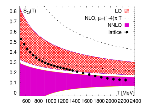
We determine the renormalization constant for the free energies by applying the direct renormalization scheme to the Polyakov loop. This procedure is covered in detail in Ref. Bazavov et al. (2016). We obtain a set of initial values of from the static energy and include the new ensembles with Bazavov et al. (2018). Here, the potential is fixed to the value with , , and . The Sommer scale and the scales and are defined through , , and . We repeat the direct renormalization procedure of Ref. Bazavov et al. (2016) after including all new ensembles. Because of the availability of higher at and for larger , we do not require iterative direct renormalization anymore. We choose those with smaller uncertainties if multiple ensembles with the same and are available. In Table 10, we summarize the new results for with substantially reduced uncertainties. Results for omitted are commensurate with from Table V in Ref. Bazavov et al. (2016). As mentioned in Sec. II, we renormalize and by adding twice the renormalized single quark free energy to and . Including the new ensembles, we repeat the extrapolation to the continuum limit (using global fits including and scaling) (cf. Ref. Bazavov et al. (2016)). In the high temperature region , we obtain a continuum limit that is reliable up to with on 95 degrees of freedom after including the full uncertainty of in the global fit. For higher temperatures, the continuum extrapolation is not reliable due to lack of data with . From , we can calculate the entropy of a static quark
| (36) |
In Fig. 18, we show the continuum limit of , which agrees with the weak-coupling result at next-to-next-to-leading order (NNLO) for . The values for in the renormalization of the free energies are taken from the same continuum extrapolation.
Appendix B CUTOFF EFFECTS AT SHORT DISTANCES
In this Appendix, we discuss the details of the improvement procedure for reducing the cutoff effects at small separations of only a few lattice steps, i.e., , which are due to the explicit breaking of the rotational symmetry in the discretized theory. We develop this procedure for the static energy at zero temperature and apply its result to the quark-antiquark (and singlet) free energies. Lattice results for the static energy are discussed in detail in Refs. Bazavov et al. (2012, 2014a, 2018). In Sec. B.1, we analyze cutoff effects in the static energy for the tree-level interaction and the tree-level improvement. In Sec. B.2, we analyze cutoff effects in the static energy for the full interacting theory with the HISQ action and nonperturbative improvement. In Sec. B.3, we apply these corrections to the free energies under study in this paper and give a quantitative account of the nonperturbative improvement that we achieve.
B.1 Cutoff effects for the tree level interaction
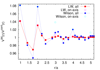
Our understanding of the cutoff effects in the static energy of a pair is largely based on the calculation at the tree level, i.e. for one-gluon exchange without a running coupling. We use this to estimate the cutoff effects on the static energy calculated with the HISQ action for .
Using the lattice version of the temporal gluon propagator , it is straightforward to calculate the tree-level static energy on the lattice, which is given by
| (37) |
The above equation defines the improved distance . Sometimes, in the following, to remark the difference from the bare nonimproved distance , we will indicate the latter with . In Fig. 19, we show the static energy at tree level calculated for the standard Wilson gauge action and for the improved Lüscher-Weisz (LW) gauge action, normalized by the continuum result of . Because of the breaking of rotational symmetry on the lattice, we have to distinguish between on- and off-axis separations. Most of the separations shown in the figure are off-axis. For the values of , which correspond to both on- and off-axis separations (e.g., ), the average of the two is shown. As one can see from the figure, cutoff effects are largely reduced for the improved gauge action and they are very small for . We use the tree-level result to reduce cutoff effects in the lattice calculations, namely, for each value of , we perform the replacement . This is called the tree-level improvement.
B.2 Cutoff effects in the static energy calculated with the HISQ action
| : | ||||||
| a (fm) | #TUs | #MEAS | Ref. | |||
| 6.664 | 0.117 | 0.0514 | 4000 | 400 | Bazavov et al. (2012) | |
| 6.740 | 0.109 | 0.0476 | 4000 | 800 | Bazavov et al. (2012) | |
| 6.800 | 0.103 | 0.0448 | 4000 | 400 | Bazavov et al. (2012) | |
| 6.880 | 0.095 | 0.0412 | 8200 | 820 | Bazavov et al. (2012) | |
| 6.950 | 0.089 | 0.0386 | 19400 | 1940 | Bazavov et al. (2012) | |
| 7.030 | 0.082 | 0.0356 | 7800 | 780 | Bazavov et al. (2012) | |
| 7.150 | 0.070 | 0.0320 | 4047 | 667 | Bazavov et al. (2012) | |
| 7.280 | 0.065 | 0.0284 | 3978 | 650 | Bazavov et al. (2012) | |
| 7.373 | 0.060 | 0.0250 | 4623 | 1000 | Bazavov et al. (2014a) | |
| 7.596 | 0.049 | 0.0202 | 4757 | 1000 | Bazavov et al. (2014a) | |
| 7.825 | 0.040 | 0.0164 | 4768 | 1000 | Bazavov et al. (2014a) | |
| : | ||||||
| a [fm] | #TU | #MEAS | Ref. | |||
| 8.000 | 0.035 | 0.01299 | 4616 | 1000 | Bazavov et al. (2018) | |
| 8.200 | 0.029 | 0.01071 | 4616 | 1000 | Bazavov et al. (2018) | |
| 8.400 | 0.025 | 0.00887 | 4616 | 1000 | Bazavov et al. (2018) | |
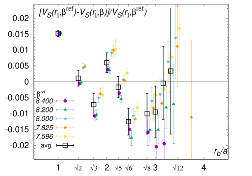
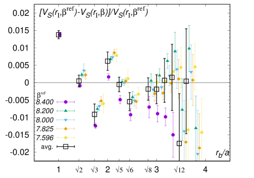
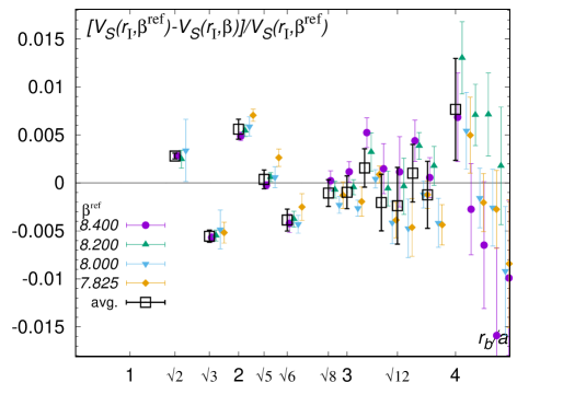
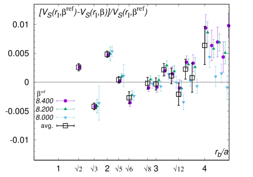
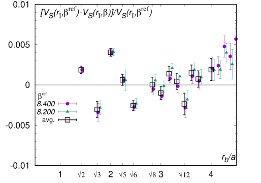
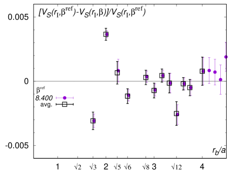
The cutoff effects in the static energy with HISQ action have been studied in Ref. Bazavov et al. (2014b). It has been shown that for the HISQ action the cutoff effects follow a similar pattern as in the free theory, namely, cutoff effects are about the same and are very small for . Using the tree-level improvement, the cutoff effects can be reduced to 1% or less (cf. Fig. 2 of Ref. Bazavov et al. (2014b)). To reduce the cutoff effects even further, we follow the procedure outlined in Ref. Bazavov et al. (2014b), but implement new refinements, which are possible due to the fact that lattices for , and are available by now. We describe these refinements in the following.
In Ref. Bazavov et al. (2014a), the static energy has been calculated for lattice spacings down to for . In the recent study Bazavov et al. (2018) of the QCD equation of state, the static energy was calculated for lattice spacings down to with , and it was shown that the quark mass effects on the static energy are negligible at distances . The lattice spacing was fixed using the scales or with and . The lattice parameters for the static energy calculations are summarized in Table 11. The static energy calculated on a finer lattice with can be used as a reference to estimate the cutoff effects in the static energy on any coarser lattice with smaller values of . By using the improved distance, we account for the tree-level cutoff effects in this comparison. More precisely, the static energy for at provides a continuum estimate of the static energy that lattice data at smaller can be compared to. To compare the static energies calculated at different values, one has to use the renormalization constants given in Table 10. However, the results of the renormalization constants are not sufficiently accurate for comparison of the static energies at subpercent precision. Therefore, we have to shift the reference static energy by a constant within the errors of the renormalization constant for such that the ratio of the potential is close to unity in the distance range , where cutoff effects are small.
Since we only have the static energy at discrete sets of data points for , we must interpolate between the data using the improved distance . The simplest interpolating function is the Cornell potential, , and it was used in Ref. Bazavov et al. (2014b). However, now we find that it is not sufficiently flexible to provide accurate interpolations. So we modify the Cornell Ansatz and supplement it by a polynomial in up to sixth order. We also try a simpler form, namely, , which works well in some cases. We also try a spline fit of . We interpolate the data for , assuming that cutoff effects are small enough to permit an interpolation with percent level accuracy. In order to extend the available range to smaller and, hence, to determine estimates of the cutoff effects at smaller separations, we extrapolate towards 10% smaller separations, i.e. down to . We estimate the continuum limit with the modified Cornell Ansatz and estimate the systematic uncertainty from the difference between fits with this modified Cornell Ansatz and the spline Ansatz. We add the statistical and systematic errors in quadrature.
Some sample results demonstrating this analysis are shown in Fig. 20. We define the correction factors
| (38) |
and observe significant deviations of from zero for , although these become smaller for finer lattices. Up to an overall sign (due to normalization) and are quite similar, although deviations from zero in Fig. 20 are smaller than deviations from one in Fig. 19. In principle, we could divide the lattice data by for any choice of to remove the residual cutoff effects. The finest lattice, i.e. in the present case, can be used as the reference lattice to estimate the cutoff effects in the static energy for any other value of . In the analysis of Ref. Bazavov et al. (2014a), only the finest available lattice with had been used. However, this approach is not optimal for a number of reasons. First of all, the same distance in physical units on a finer lattice corresponds to a larger number of lattice steps than on a coarser lattice. Thus, the signal-to-noise ratio for the same physical distances is worse for finer lattices than for coarser lattices. Second, for larger distances, , the lattices with smaller light quark mass should be used to avoid systematic errors due to using different quark masses. Finally, the continuum estimates for different suffer from independent statistical fluctuations, which may be reduced by combining different . This leads to a procedure with strong similarities to step-scaling techniques. We vary the reference lattice from to and determine estimates for the cutoff effects for lattices with .
For small distances on the finer lattices, is fairly independent of the choice of . However, Fig. 20 shows that this observation does not hold similarly well on coarser lattices and for larger distances on the finer lattices. The spread between different determinations of for different continuum estimates, i.e. different , can be understood as follows. The spread becomes larger for distances where the renormalized static energy is close to zero and, thus, the ratio in Eq. (38) suffers from large fluctuations. Nevertheless, the overall pattern of the short distance cutoff effects does not change for different choices of . Hence, we determine a weighted mean from with different using squared errors as weights. We obtain errors for from the (weighted) variance and from weighted averages of the errors of the . We add both types of errors in quadrature and show these in Fig. 20.
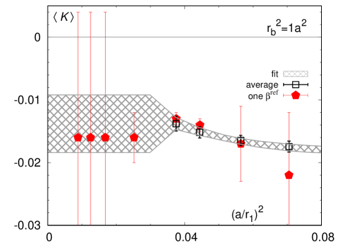
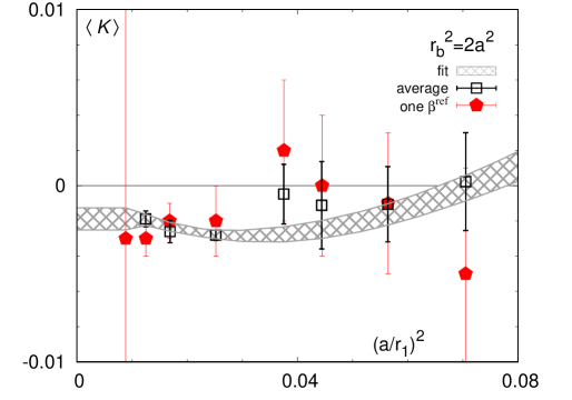
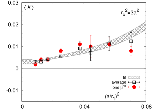
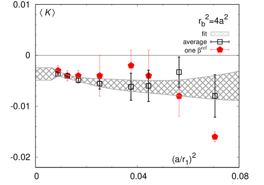
After determining the -averaged correction factors , we put together sets of for different lattice spacings and interpolate between these. For each , we use an Ansatz of the form
| (39) |
where terms can be omitted because the tree-level improvement discussed above removes lattice artifacts of order . Moreover, as a term would persist in the continuum limit where rotational symmetry is not broken, such a term is forbidden. We perform a bootstrapped fit and vary the number of higher order terms kept in Eq. (39). We accept only fits for which we obtain and use their mean as our final interpolation result and the mean of their bootstrap errors as the final statistical error. If we do not obtain fits with reasonable , we successively omit the last point at the small end–the coarsest lattice–and repeat the same set of fits (only for we had to omit the last point in order to obtain a smooth interpolation). We estimate the systematic error of the interpolation as the variance of the set of accepted fits. The final is then obtained from the final fit and the input data using an average of the degrees of freedom for the set of accepted fits. We show some sample results of this interpolation in Fig. 21, which describe quite well for all considered lattices.
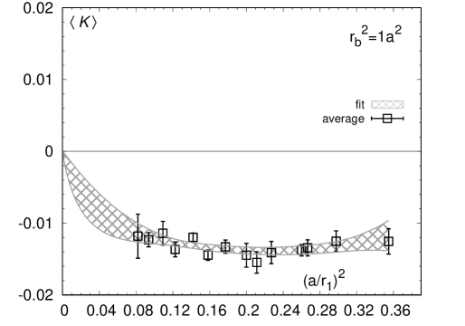
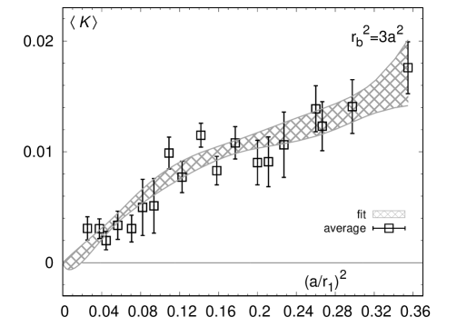
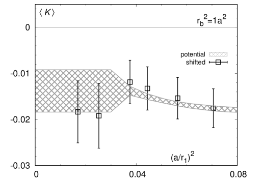
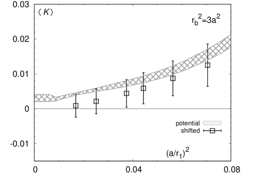
However, we do not always see an unambiguous onset of scaling behavior for very fine lattices. This may indicate that the correction factors do not approach the continuum limit smoothly. For this reason, we conservatively estimate that the last that we can obtain applies for any larger and assume a 33% relative systematic uncertainty. For all values of , we observe a strong increase in the fluctuations of for the coarsest lattices. This effect is due to the choice of the renormalization scheme, in which for such distances. We address this growth of fluctuations by using an alternative renormalization scheme, namely, we shift the static energy by with respect to the usual potential scheme. Thus, we defer and the growth of fluctuations to substantially larger distances. In this scheme, we can determine correction factors for the previously problematic range without a large growth of the errors. We repeat the same type of analysis in the shifted renormalization scheme, but use as reference lattices. We observe here that errors seem to be underestimated in the range , which corresponds to . We require that the averaged correction factors have relative errors of at least 5% for in order to obtain stable fits. We show some sample results in Fig. 22. is significantly smaller in the shifted scheme and the growth of for coarse lattices has been much diminished. In order to compare to the original potential scheme, we have to convert the correction factors back to the original scheme. We show the comparison between both schemes in Fig. 23. The typical differences between both determinations of are about 0.2%-0.4%, but are mostly covered by the statistical errors that remain after converting the shifted scheme back to the standard renormalization. The fair agreement between both schemes indicates that the cutoff effects have been identified appropriately and the systematic error due to scheme dependence is about 0.2%.
If we can determine for given and , we assign this systematic error of 0.2% to any data (in the following, denoted as ), which we add in quadrature to the statistical error. If we fail to obtain at the same for larger and at the same for smaller , we assume that we have reached the limit of the validity of a controlled determination of . In these cases, we refrain from using the correction factors and instead double the statistical error and add a 1% relative error in quadrature. If the data are too close to zero, i.e. , we add an additional systematic error estimate of absolute to . In a case where we cannot determine a correction factor at all (for the coarsest lattices, i.e. ), we double the statistical error and add a 2% relative error in quadrature. If the data are too close to zero in these cases, i.e. , we add the same additional systematic error estimate of absolute to . At last, we take a weighted average of the corrected results obtained in both schemes using the squared errors as weights. We use the same weights for averaging the errors and add the difference between both as systematical error in quadrature.
Subsuming the aforementioned considerations in our definition of , we define the improved static energy as
| (40) |
for fine lattices, i.e., , is usually within . The first point, , which also has the strongest tree-level correction, , is an exception with . Combined uncertainties due to statistical errors of the bare static energy and due to systematic errors of the correction factors are usually smaller than relative error for fine lattice spacings. Although the latter are the dominant -dependent source of uncertainty, errors due to renormalization with are much larger than those due to correction for the cutoff effects on fine lattices.
B.3 Improvement at finite temperature
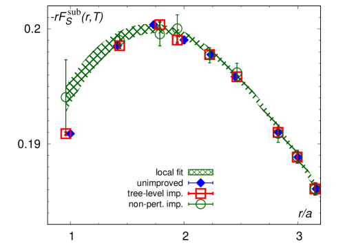
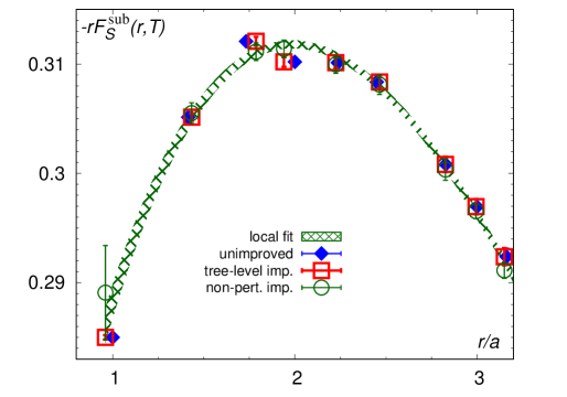
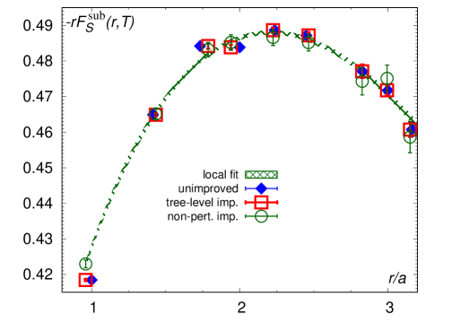
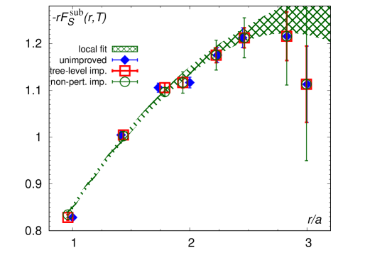
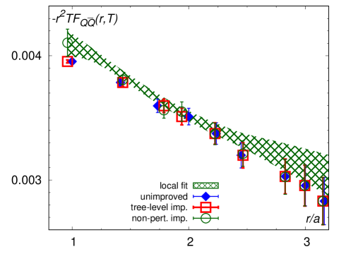
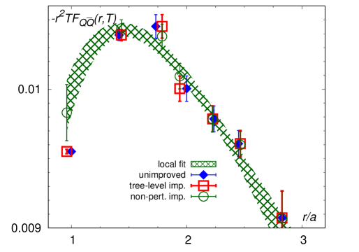
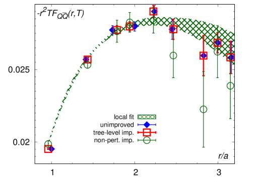
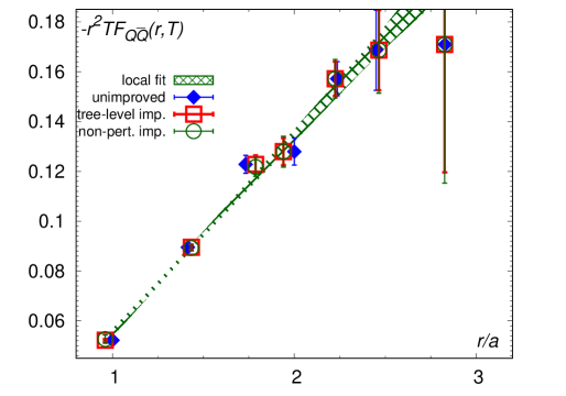
The improvement procedure that we have developed so far is only relevant for cutoff effects at short distances, where short is meant in terms of only a few units of the lattice step, i.e. typically . When looking at short distances for finite temperature observables, we usually mean short in units of the inverse temperature, i.e. , respectively, . In the following, we argue why the same short distance improvement is appropriate for static correlators at finite temperature. At the shortest distances cutoff effects usually exceed the small statistical errors of the free energies and cause nonsmooth behavior. This is a major problem for smooth interpolations including short as well as larger distances.
In Sec. IV, we have shown that the singlet free energy is vacuumlike up to small corrections for . Thus, we expect to obtain a similar improvement with the correction factors that have been determined for the static energy at . Namely, we define
| (41) |
However, for , it is not obvious if these improvement procedures are appropriate, since is already within the electric screening regime. We show a few sample singlet screening functions with tree-level or nonperturbative improvement and without improvement in Fig. 24. For , modifications due to improvement are small compared to medium effects and do not alter the result significantly. On the finer lattices, i.e., , improvement smoothens the short distance regime for and substantially helps with obtaining interpolations of the data. The systematical uncertainties of the improvement factors are usually at least as large as the statistical errors of the finite temperature results at short distances. These larger errors are beneficial for smooth interpolations of the improved data. Since we use the same tree-level and nonperturbative corrections for and , we expect that leading corrections are subject to strong cancellations in the difference . We simply use unimproved distances and omit nonperturbative correction factors.
In Sec. V, we have shown that the Polyakov loop correlator can be understood through its decomposition into color singlet and octet in pNRQCD for at all temperatures in the study. Using Eq. (30), we can obtain a correction prescription for on the basis of the correction factors for the static energy. We write the improved normalized Polyakov loop correlator in terms of the improved static energies, neglecting any Casimir scaling violations,
| (42) |
We know and we can use to expand in , eventually obtaining
| (43) |
The need for corrections and the validity of the pNRQCD formula are both restricted to short distances. In this range, we have seen that the reconstruction using works as well as using , but provides access to the full range. Hence, we replace by to obtain our final expression
| (44) |
which is valid to leading order in . We show a few sample screening functions with tree-level or nonperturbative improvement and without improvement in Fig. 25. The effects of improvement are hardly relevant for on most lattices. In the cases where these effects are visible, the corrections generally lead to a smoother free energy at short distances.
Appendix C INTERPOLATIONS AND EXTRAPOLATIONS
In this Appendix, we discuss the details of the interpolations of the subtracted quark-antiquark (and singlet) free energies and how we extrapolate (and ) to the continuum limit. We do not repeat here the discussion of the physical underpinning of the presented analysis, which we discuss in detail in Sec. III.1. Here we also discuss the interpolations and extrapolations of . In the following, we refer to either or just as the free energy unless we apply different treatment to both and use these quantities in temperature units, namely, we fit and . This Appendix also covers the calculation of the derivative of . We usually propagate statistical errors through the fits by generating 100 bootstrap samples of mock data assuming Gaussian errors and perform the fits on the mock data. We perform fits using either linear regression, the built-in smoothing splines of the R statistical package R Core Team (2018), or use for nonlinear fits the nlme package Pinheiro et al. (2018).
We arrive at our continuum result through the following procedure.
- 1.
-
2.
We interpolate in and using two different data-driven schemes. We use local fits in the first scheme and global fits in the second scheme.
-
3.
We calculate weighted averages of the results from the two schemes and estimate systematic errors due to model dependence.
-
4.
We extrapolate the combined results to the continuum limit for each individual point using different subsets of the and different Ansätze for scaling behavior.
-
5.
After inspecting scaling behavior for sets of representative points, we compile the final continuum result using different extrapolations in those regimes where they are appropriate.
-
6.
Finally, we obtain the renormalized continuum result by adding (cf. Appendix A).
As stated, we follow a data-driven scheme in fitting the and dependence. Namely, we iteratively try to find the most simple, smooth function of that incorporates the main features known from weak-coupling results (LO short distance behavior and exponential damping) and describes the largest subset of the statistically relevant data. We reduce the fit range at the large distance end in small steps if we fail to fit the data with any reasonable choice of smooth function. If the data set becomes too short, the statistical errors of the data at the shortest distances and of the nonperturbative corrections must have been underestimated. This implies that data are nonsmooth at the shortest distances. In these cases, we have to enlarge the errors of all data by a small amount that permits a smoother curve and restart the procedure. We end the procedure when meeting a stopping criterion in terms of both the residues at the shortest distance and globally and in terms of a reasonable determination of the propagated errors of the interpolating function. We discuss the stopping criteria for each of the fits in the following sections.
C.1 Local fits
We perform local interpolations first in the quark-antiquark separation and later in the temperature. For the former, we explicitly account for correlations between data at different separations obtained within the same gauge ensemble by fitting on the individual jackknife bins. We have tested that a different ordering of the fits, i.e. first interpolating in the temperature for fixed distances and then interpolating in the distance for fixed temperature, does not change the results in a statistically significant way. However, the latter ordering does not permit one to account for the correlations within each ensemble.
C.1.1 Distance interpolations
We independently interpolate or rather as a function of for each and each . We split the data into intervals of small and large separations, where we treat the first 16 points as data at small separations and the rest including some overlap region as data at large separations. Before interpolating data at large separations, we calculate residues at large separations by extrapolating with the fit to data at small separations. The residues are computed with data at large separations that did not enter into the fit at small separations. If these residues satisfy ( being the data at large separation), we forgo the separate interpolation at large separations and just use the extrapolation. If we have separate interpolations for small and large separations, we match the two interpolations smoothly.
For the local fits, we assume smoothness and screening of the subtracted free energies and use a modified, screened Cornell potential (MSCP) Ansatz
| (45) |
We keep a parameter to account for a possible offset due to incomplete cancellation in the subtraction of , but also try the same fits with , i.e. omitting the parameter altogether. We demand that the screening mass parameter is positive, but also try fits with for low temperatures, i.e., . We generally use and limit the number of monomials by if enough data points are available. If we fit for small separations with at least six data points and not very high temperatures, namely, with at most , we limit the minimal number of monomials as . Otherwise, we use . In the denominator, we choose at short distances for due to the form of the LO result [Eq. (32)], and for . At larger separations, we use both for and . Lastly, we use for . In the latter case, we also limit the range to for and to for . Because of the small size of the gauge ensembles for , we enlarge the corresponding statistical errors by a relative error estimate.
We vary and thus perform nonlinear fits for different polynomial orders in order to choose the most simple Ansatz that matches the data for short or large separations. In a first cycle, we interpolate only the jackknife average to determine an appropriate fit function that permits meeting a stopping criterion. In a second cycle, we perform the interpolation on all jackknife bins, thus taking correlated fluctuations of data into account and propagating the statistical errors. If the need arises, we readjust the fit function as in the first cycle. We estimate the bias from the difference between the average of the fits on the individual bins of data and the fit on the average of the bins of data and add the bias to the statistical error in quadrature. As stopping criterion of the loop, we demand that the fit converges on at least 20% of all bins with 555We use this purely heuristic limitation for acceptable to accelerate the process of identifying underestimated systematical errors and finding appropriate interpolating functions. and that–after we exclude fits on bins with from an average–the average of the fits satisfies . If we reach small enough for some , we also attempt a fit with polynomial of order with the constant term omitted. Between these, we choose the fit with smaller .
We perform a nested loop over different fits starting from the minimal permitted and increase towards the maximal permitted in an inner loop. If we fail to meet the stopping criterion, we omit points and restart the inner loop. For small (large) separations, we omit points at the large (small) end of the fit range. If we fall below nine data points in this process, we restore the full fit range, but add a systematical error estimate on top of the previous errors to the data. We add 0.5% times the minimal of the recent inner loop as relative error estimates and restart the inner loop. If we fail to fit for small (large) separations with at most 20% (30%) relative error added, we consider the fit as a failure. We restart the outer loop without a screening mass parameter for small separations at low temperatures, i.e. , reasoning that we do not have enough data to resolve screening as well as subleading terms in the polynomial. For small separations, we aim at fits with sufficiently small residue on the first point. If we cannot achieve , we restart the outer loop and permit or even . We can always get acceptable fits under the latter condition. We use the fits for large separations to extrapolate up to the first point, where the fit to becomes compatible with zero within errors.
We test for model independence of the fit procedure by performing smooth spline fits to fits with 100 bins of bootstrap mock data treating all errors as independent. For the latter, we use as few knots as possible and a smoothing parameter as large as permissible to still obtain . We find fair agreement between all these fits within their respective uncertainties, albeit with underestimated errors for the bootstrapped nonlinear fit and with overestimated errors for the spline fit. We consider the MSCP fits on the jackknife bins as our final local interpolation of . We obtain the derivative analytically for every fit function and insert the fit parameters on the individual bins to compute the average and propagate the errors.
For , we follow more or less the same procedure. We omit the screening mass altogether and do not use jackknife bins, since we obtain by subtracting jackknife averages of statistically independent data sets whose sizes may differ substantially. In practice, the actual fluctuations appear to exceed the statistical errors, which have been added in quadrature. Since many data for are very close to zero, we demand that absolute errors666Since for very small distances and high temperatures, see Sec. IV.1, this enlarged error cannot create fake plateaux at short distances. are at least . In the case of enlarging the errors, we add times the minimal of the recent inner loop as absolute error estimates and restart the inner loop. We do not extrapolate to larger separations here. Other than these, the local fits to follow the same procedure as the fits to .
C.1.2 Temperature interpolations
In the next step, we independently interpolate the MSCP-interpolated results for or in for each and fixed . We perform separate temperature interpolations for the derivatives. We use smoothing spline interpolations that penalize higher derivatives. We require for the internal smoothing parameter () of the built-in smooth splines of the R statistical package R Core Team (2018) for and for the derivatives. We limit the maximal smoothing parameter for the temperature interpolations to and include data for all available temperatures. We perform separate interpolations in overlapping low () and high () temperature intervals. If the fits yield , we enlarge the errors of the input by a factor Here we have to stress that the input for these interpolations are intermediate mock data, whose errors may have been underestimated. If the fits in these intervals fail to produce 777This restriction is heuristic. When enlarging the errors after obtaining , the fits generally fail to reproduce the input values in the overlap region well. without enlarging the errors, we remove the highest (or lowest) temperature in the overlap region from the fit and repeat the fits. We always keep at least one temperature common between both fits. This procedure is necessary since data at very low temperatures usually have much larger uncertainties than at higher temperatures. Thus, a global interpolation cannot resolve the increase of towards low temperatures properly. In agreement with predictions of weak-coupling results (cf. Secs. IV and V), the dependence is much flatter at higher temperatures than at lower temperatures. In the overlap region, the second derivative is quite large, and thus, use of a smoothing parameter penalizing higher derivatives is hardly appropriate. In the full overlap region, we match the fits for low and high temperatures smoothly.
C.2 Global fits
We perform separate global fits to the free energies and to for each . For the free energies, we perform the fits over the full temperature range as well as for low or high temperature intervals with or , respectively. Because of the small size of the gauge ensembles for , we enlarge the corresponding statistical errors by a relative error estimate. For , we limit the range to for and to for , but fit all available temperatures at once. In order to obtain stable fits, we have to enlarge the errors of to 5% relative error or absolute error, whichever is larger.
For the global fits, we use a generalized temperature-dependent modified screened Cornell potential (GTDMSCP) Ansatz. In the GTDMSCP Ansatz we generalize Eq. (45) as
| (46) |
We did not observe any systematic temperature dependence in the values of from local fits using the MSCP Ansatz [Eq. (45)]. Hence, we must omit in the global fits and consider effects leading to in the local fits as temperature-dependent uncertainties that have to be averaged out in the global fit. In the GTDMSCP fits, we assume that the dominant temperature dependence is in the double polynomial, while we assume that the temperature dependence of the screening mass is rather mild.888In our conventions the screening mass is a screening mass in units of the temperature, namely is the screening mass in physical units. This trivial multiplicative temperature dependence is taken out in our Ansatz. We model the temperature dependence of the screening mass as
| (47) |
where we restrict the range of to the interval and normalize the temperature logarithm by to ensure a relatively mild temperature dependence of . This choice of restricts the logarithm to about , which is sufficiently flexible to permit even negative screening masses at one end of the temperature range. As we typically obtain in fits, our model is sufficiently flexible. Unless it comes out as zero, is generally positive and larger than by an order of magnitude.
To model the dominant temperature dependence in the GTDMSCP Ansatz in a very general form, we use sequences of consecutive powers of the temperature and vary the lowest and highest powers. We use between and and sequences with lengths . After rescaling the temperatures as , we obtain mostly coefficients of natural size. We construct all consecutive sequences including and iteratively increase when needed. We use as the highest power of , but observe that the global fits generally favor lower powers of . As leading inverse power of , we use for and for . The underlying reasoning for this choice is the form of the LO result [Eq. (32)].
| range | range | ||||
|---|---|---|---|---|---|
| 4 | 0% | 1032/930 | |||
| 6 | 0% | 96/133 | |||
| 6 | 0% | 1609/1463 | |||
| 8 | 0% | 270/286 | |||
| 8 | 0% | 1558/1877 | |||
| 10 | 0.9% | 221/217 | |||
| 10 | 0% | 2397/2049 | |||
| 12 | 0.5% | 170/202 | |||
| 12 | 0% | 2398/2067 | |||
| 16 | 1.0% | 1315/1185 |
| range | range | ||||
|---|---|---|---|---|---|
| 4 | 0% | 350/387 | |||
| 6 | 0% | 163/169 | |||
| 6 | 0% | 723/695 | |||
| 8 | 1.2% | 190/264 | |||
| 8 | 0% | 603/849 | |||
| 10 | 1.2% | 227/199 | |||
| 10 | 0% | 1025/923 | |||
| 12 | 0% | 103/120 | |||
| 12 | 0% | 944/821 | |||
| 16 | 1.0% | 290/386 |
| range | range | ||||
|---|---|---|---|---|---|
| 4 | 0% | 59/134 | |||
| 6 | 0.8% | 188/136 | |||
| 8 | 0.5% | 353/297 | |||
| 10 | 0.5% | 404/313 | |||
| 12 | 0% | 340/330 |
We perform nonlinear fits for different choices of and to determine the most simple Ansatz that matches the data. We use three nested loops for searching the optimal fit function. The two outer loops are the same as for the local fits, while the innermost loop is the loop over the sequences of consecutive powers of . In a first cycle, we perform the global fits on the jackknife average to identify an appropriate fit function. In a second cycle, we use bootstrap mock data to propagate the statistical errors. If the need arises, we readjust the fit function in the second cycle again. If we fail to reach convergence, we add 0.5% times the minimal of the recent loop and restart the outermost loop. We observe that we almost universally need sequences from to and sometimes in addition . For this reason, we eventually start from sequences of length for our final fits. With regard to the dependence, we demand for the free energies at least two and at most three terms beyond the leading powers. We summarize the global fits of and in Tables 12 and 13. Requirements for powers of the polynomials, enlarged errors, and achieved results are quite similar for the local fits.
For , we omit the screening mass completely and demand at least three terms beyond the leading power, which we fix through . As discussed in the subsection on local fits, appears to be affected by fluctuations that are larger than the statistical errors. In order to obtain stable interpolations, we have to enlarge the errors globally to the larger of absolute error or relative error before fitting. We summarize the global fits of in Table 14.
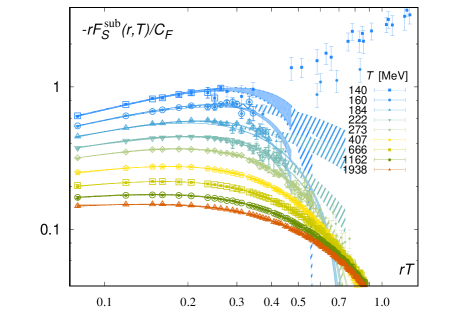
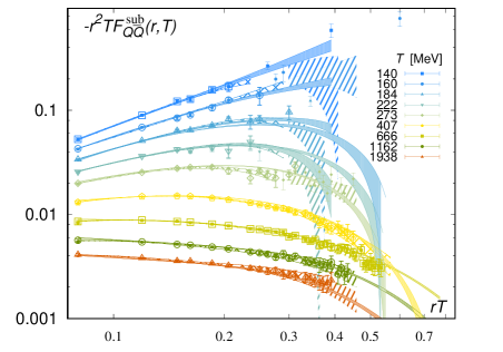
In Fig. 26, we show a comparison of the low and high temperature global fits and the corresponding local fits before temperature interpolation with the underlying data for . Within the range of fitted data for we obtain fair agreement between local and low temperature global fits, but not with the other global fits. For , we find fair agreement between local and global fits for high temperatures or on the full temperature range. Therefore, we switch for from the low temperature fits to the high temperature fits. We estimate systematical errors of the global fit from half of the difference in the range and add it to the statistical error. We obtain the and derivatives analytically for every fit function and insert the fit parameters on the individual bins to compute the average and propagate the errors.
C.3 Average of local and global fits
The assumption of smoothness in the temperature leads to substantially smaller errors in the interpolating functions than in the actual data (see Fig. 26). Hence, we assume that the errors of the interpolating function may be underestimated and we have to account for that. This is particularly relevant at the shortest and largest distances. At the shortest distances, there are only a few points with relatively large systematic errors, which have only little weight in the global fits. At the largest distances, the local fits are oblivious of the smoothness condition between neighboring temperatures and are sensitive to incomplete subtraction. These complementary systematic uncertainties can be directly observed in Fig. 26.
We eventually calculate the weighted average between the local and global fits before the continuum extrapolation. The former do not require that the subtracted free energies approach zero at large , while the latter do not require that the screening mass parameter is positive. Hence, they have different systematic uncertainties for large , which can be controlled better through an averaging procedure. We estimate the systematical error from the difference between local and global fits. , We restrict the growth of the error of the averaged result such that the band of the averaged result is contained by the combined bands of the local and global fits. Moreover, to account for any remaining uncertainties at short distances we demand that the relative error must not be smaller than the difference between relative errors of the corrected and uncorrected data for the nearest point in the plane.
This is still not sufficient for a reliable continuum extrapolation. We find that quite often interpolated data with , and sometimes are in the scaling window, while some interpolated data for or are not consistent with this scaling behavior (see the scaling plots in Sec. C.4). This is direct evidence that interpolations with still have underestimated uncertainties. For this reason, we enlarge the errors of interpolations by hand for . We add to interpolations with a 1% relative error for and a 2% relative error for . We add to interpolations with a 0.5% relative error for and a 1.5% relative error for .
C.4 Continuum extrapolations and error estimates
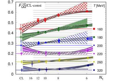
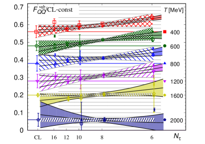
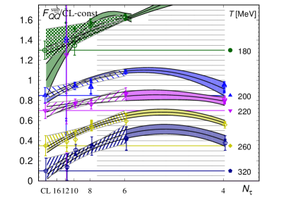
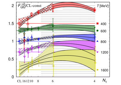
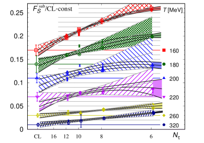
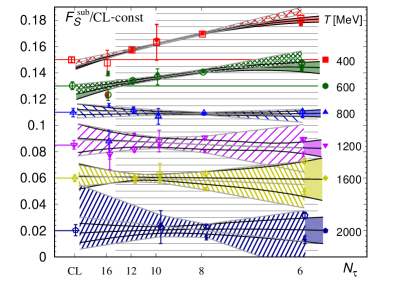
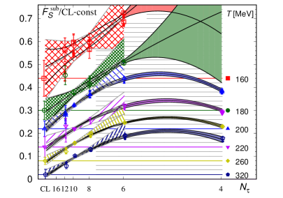
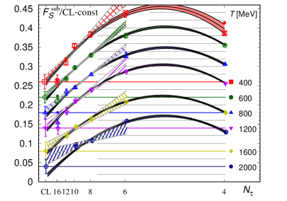
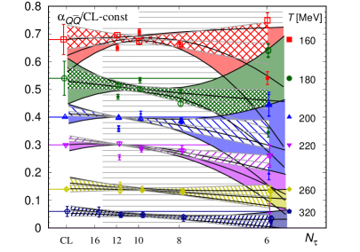
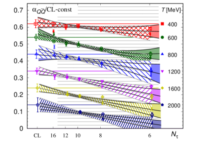
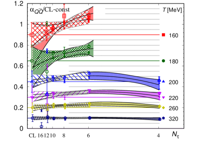
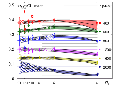
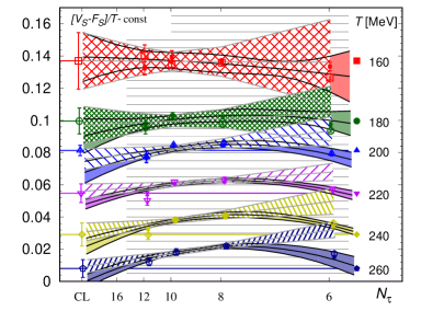
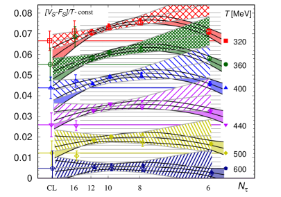
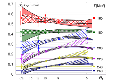
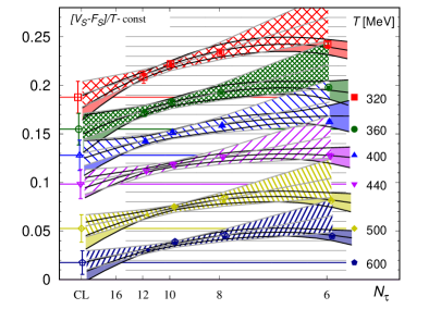
We extrapolate the subtracted free energies and , the derivative (and thereby ) and to the continuum limit. With all continuum extrapolations, we attempt to cover as much of the plane as we can control with reasonable uncertainties. In particular, since we are interested in the different regimes of the interactions, we have to anticipate a drastic variation of the cutoff effects of each quantity depending on the region of the plane. Moreover, depending on the region, we have very different subsets of the data available. Namely, for small separations, we can use only fine lattices with large , and for large separations, we have only data with smaller due to the increasing noise problem with larger . For these reasons, we must assume that a global continuum extrapolation may fail to reflect the associated uncertainties of the data as well as the richness of the underlying physical structures appropriately. Instead, we perform independent continuum extrapolations using the averaged, interpolated results for each point of the plane.
| 8, 10 | 12, 16 | 0 |
| 6, 8, 10 | 12, 16 | 2 |
| 4, 6 | 12, 16 | 4 |
Because of the structure of the HISQ/tree action, the leading cutoff effects are . Since we take the continuum limit at fixed temperature and , this translates into a parametrization of leading cutoff effects through inverse powers of . We use the Ansatz
| (48) |
and vary the set of values that are included in the fit. Furthermore, we either use just the term (assuming data are already in the continuum limit within errors), or include the term, assuming scaling. In extrapolations that include data with or , we also include the term. As we perform independent continuum extrapolations, we do not make any assumptions about the dependence of , and . For this reason, our continuum extrapolations do not necessarily yield a smooth function in the plane. We list the different types of fits used for continuum extrapolation in Table 15. If the number of data with different exceeds the number of parameters of the interpolating function, we perform a linear regression fit and directly propagate the errors. After propagating the errors through the linear regression, we rescale them by in cases where we obtain . Occasionally, this may lead to large spikes in the error of the continuum result if the underlying data are aligned particularly well due to fluctuations. Otherwise, we estimate the errors of the continuum limit with bootstrap mock data. We instead omit if we have only three different available.
We have to consider the possibility that the sequential interpolations or the global fits together with the average and systematic error estimates may still underestimate the actual uncertainties of the correlators. If necessary, we enlarge the errors (of the averaged data underlying the continuum extrapolation) to reach . For each datum, we determine in the plane the closest point of the nonperturbatively corrected data set for the same . We permit enlarging the relative error of the averaged result up to the relative error of this closest corrected original datum. We simultaneously enlarge errors of the results for all in four steps up to the permissible maximum for each and repeat the fit.
In Figs. 27–30, we show the approach to the continuum limit for the various free energy observables, usually in terms of a ratio of the lattice result over the continuum limit. We show two representative distances: one in the vacuumlike regime and one in the electric screening regime. We have shifted the ratios for different temperatures vertically for better visibility. The colored horizontal lines indicate the continuum value for each temperature to facilitate reading off the size of the cutoff effects for each .
| or | 0.5 | |
| or | 1.0 | |
| or | 2.0 | |
| or | 0.5 | |
| or | 0.5 | |
| or | 0.5 | |
| or | 0.5 | |
| or | 0.5 | |
| or | 0.5 | |
| or | 0.5 | |
| or | 0.5 | |
| or | 0.5 | |
| or | 0.5 |
We show the approach of to the continuum limit for a few representative pairs in Fig. 27. In general, we see that within an -scaling window decreases towards the continuum limit and that -scaling contributions come with opposite sign. Within numerical uncertainties, with is always inside the -scaling window for , while with is never inside the -scaling window. In general, we see that the approach to the continuum limit becomes steeper for lower temperatures and larger separations and flatter for higher temperatures and shorter separations, i.e., cutoff effects become larger from the upper left to the lower right corner of the plane. For small distances up to , cutoff effects are at most a few percent or not even unambiguously resolved at all. For intermediate distances up to , cutoff effects grow up to about 20% in the transition region and 5% for temperatures beyond . For large distances beyond , cutoff effects are even larger, 30% and more for , and stay at such level even for the highest temperatures. We summarize in Table 16 which continuum extrapolations we combined in our final result for .
| or | 1.0 | |
| or | 0.5 | |
| or | 1.0 | |
| or | 0.5 | |
| or | 0.5 | |
| or | 0.5 | |
| or | 0.5 | |
| or | 0.5 | |
| or | 0.5 | |
| or | 0.5 | |
| or | 0.5 | |
| or | 0.5 | |
| or | 0.5 | |
| or | 0.5 |
We show the approach of to the continuum limit for the same representative pairs in Fig. 28. As for we see that within an -scaling window decreases towards the continuum limit and that -scaling contributions come with opposite sign. Within numerical uncertainties, with is always inside the -scaling window for , while with is never inside the -scaling window. In general, we see as for that the approach to the continuum limit becomes steeper for lower temperatures and larger separations and flatter for higher temperatures and shorter separations, i.e. cutoff effects become larger from the upper left to the lower right corner of the plane. For small distances up to , cutoff effects are at most a few percent or not even unambiguously resolved at all. In particular, the coefficient seems to switch to the opposite sign above and . We consider this as an indication that these data may be considered in the continuum limit within errors. For intermediate distances up to , cutoff effects grow up to about 15% in the transition region and 4% for temperatures beyond . For larger distances beyond , cutoff effects are even larger and gradually increase up to 40% for at . For the highest temperatures cutoff effects are about half this size. We summarize in Table 17 which continuum extrapolations we combined in our final result for .
| or | 1.0 | |
| or | 0.5 | |
| or | 1.0 | |
| or | 0.5 | |
| or | 0.5 | |
| or | 1.0 | |
| or | 0.5 | |
| or | 0.5 | |
| or | 0.5 | |
| or | 0.5 | |
| or | 0.5 | |
| or | 0.5 | |
| or | 0.5 | |
| or | 0.5 | |
| or | 0.5 |
We show the approach of to the continuum limit for the same representative pairs in Fig. 29. Contrary to we see that within an -scaling window increases towards the continuum limit at short distances, , while it tends to decrease towards the continuum limits for larger distances. This change in behavior is clearly due to the physical regimes, namely, the vacuumlike regime and screening regime. The -scaling contributions always lead to an increase towards the continuum limit. Within numerical uncertainties, with is always inside the -scaling window. Even with is close to the -scaling window for the smallest separations. In general, we see for that the approach to the continuum limit is different in the vacuumlike regime and in the screening regime. In the vacuumlike regime, it seems to become slightly steeper for higher temperatures and some intermediate separations, while in the screening regime, it behaves rather in the opposite way. For small and intermediate distances up to , cutoff effects are at most about 5% percent or not even unambiguously resolved at all. For larger distances beyond , cutoff effects eventually change their sign and become even larger and similar to those of in terms of sign and magnitude. We summarize in Table 18 which continuum extrapolations we combined in our final result for .
| or | 0.5 | |
| or | 0.5 | |
| or | 1.0 | |
| or | 1.0 | |
| or | 0.5 | |
| or | 0.5 | |
| or | 0.5 | |
| or | 0.5 | |
| or | 0.5 | |
| or | 0.5 | |
| or | 0.5 | |
| or | 0.5 |
Lastly, we show the approach of to the continuum limit for a similar set999 Here we use bare distances instead of improved distances. Hence, is not accessible with . The temperature range is limited by the values of the available lattices. of representative pairs in Fig. 30. We cannot plot the ratio of results at finite lattice spacing and the continuum result, since data are actually crossing zero at different points in the plane. In general, we see that within an -scaling window decreases towards the continuum limit and that -scaling contributions come with the opposite sign. Contrary to , we see that the -scaling window extends only to . Although with appears to be systematically outside the -scaling window, the -scaling contribution is rather mild. In general, we see for that the approach to the continuum limit appears very flat for low temperatures, , and quite temperature independent for . Cutoff effects become systematically larger for larger separations. For small distances up to , cutoff effects are not even unambiguously resolved and data at finite fluctuate around the continuum result without clear scaling behavior. We consider this as an indication that these data may be considered in the continuum limit within errors. For intermediate distances up to and temperatures above , cutoff effects grow in size from to with increasing separation and show clear scaling behavior. For larger distances around and beyond, cutoff effects seem to stay at a similar level. We summarize in Table 19 which continuum extrapolations we combined in our final result for .
We universally find that cutoff effects at the shortest distances that we can access with multiple are consistent with zero within errors. Thus, we extend the continuum result to even shorter distances by taking the results for the (respective) largest in the extremely short range as a continuum estimate. These continuum estimates are included in the continuum results that are plotted in the figures in the main body of the paper.
C.5 Continuum estimates for results
For the continuum estimates of the zero temperature static energy we use the nonperturbatively improved results at finite lattice spacing. We use the lattices in Table 11 and the improvement procedure discussed in Appendix B.
After nonperturbative improvement, the results at different lattice spacings are consistent within their respective errors. Therefore, in the range where we have results available at multiple , each of these results is within its uncertainties in the continuum limit. For the shortest distances, , we assume that the nonperturbatively improved results on the finest lattice are consistent with the continuum limit and treat these as our continuum estimate. Instead of following a similar approach as we did for (cf. Sec. C.4), we construct our entire continuum estimate for from nonperturbatively improved results at finite lattice spacing. The three reasons for this change of procedure are that we do not have to consider - or -dependent cutoff effects, that the results on finer lattices anyways do not contribute strongly to the continuum limit at larger distances, and that the finest lattices have a larger light sea quark mass than the coarser lattices. The second reason can be understood from the fact that such distances correspond to rather large values of on finer lattices, and thus, results on finer lattices have accumulated more noise at the same distance. We construct our continuum estimate by using only points with for each lattice spacing to keep the errors small. Quark mass dependence as the third reason has been discussed already in Appendix B. By restricting the lattice results with larger quark mass to distances much smaller than , we avoid that the quark mass dependence is numerically important.
| 0.025 | 8.400 | ||
| 0.035 | 8.000 | ||
| 0.040 | 7.825 | ||
| 0.065 | 7.280 | ||
| 0.109 | 6.740 |
For the results in the figures we obtain two bands as follows. We use results with five different lattice spacings, namely, with , and . We plot the nonperturbatively corrected results for for each lattice spacing in a different range to ensure that we always use data at only a small number of lattice steps, . For lattices with , we use even shorter separations, . For the coarser lattices, we leave out the first few points, where cutoff effects are somewhat large, and thus, the nonperturbative improvement introduces a larger systematic error. The reason for these short distance cuts is that we aim at obtaining a smooth error band. We summarize this construction in Table 20 and show the corresponding result with black pentagons and a black band in Fig. 1. For the result in Figs. 2 and 4, we use a derivative of this result obtained numerically from a fit with an Ansatz as a modified Cornell potential (see App. B for a discussion of these fits).
However, this is still not enough for a comparison of from high temperatures to the limit. For this comparison, we make use of information obtained from the direct comparison between and in Sec. IV.1. Figure 6 shows that is for sufficiently small within numerical uncertainties constant and independent of the temperature for . This constant is small compared to the numerical uncertainty introduced due to the renormalization constant at high values. Hence, within the numerical errors, the renormalized result for is a fair estimate of as long as and . We employ the continuum result for in the range for , namely, for the temperatures , and , as an estimate for the zero temperature result at even shorter distances, reaching down to . This estimate for is shown as a light gray band in Fig. 1.
Appendix D FITS OF THE LARGE DISTANCE BEHAVIOR OF THE CORRELATORS
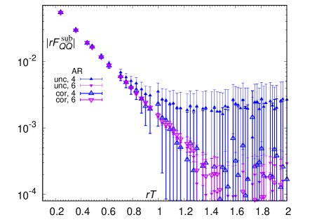
In this Appendix, we discuss the details of the analysis of the asymptotic behavior of the subtracted free energies and the extraction of the asymptotic screening masses. For this analysis, we perform fits on all jackknife bins to account for correlated fluctuations of neighboring data points. The discussion of finite volume effects in Appendix A revealed that screening functions for static quark-antiquark free energies are quite susceptible to finite volume corrections. Thus, we fit for large separations as
| (49) |
assuming that the one-particle exchange is the dominant process for large separations. The asymptotic cancellation between the squared Polyakov loop and the static quark-antiquark correlators strictly holds only in infinite volume. Hence, we account with the fit parameter for possible offsets due to an incomplete cancellation with at finite volume. We determine by fitting a constant to the asymptotic tail of . We define this tail as made of all points with signal-to-noise ratio less than one and of all points at larger . By subtracting the parameter from we account for the asymptotic finite volume corrections and bring results with different volumes into much better numerical agreement.
For , we show the effect of the correction on in Fig. 31. There, we obtain a good signal in the larger volume up to . After the finite volume correction, the central value of the result in the smaller volume sits on the top of the finite volume corrected result in the larger volume (albeit with large errors that render analysis of the last few data points moot). For different , the picture is quite similar. With the singlet free energy, we can access much larger ranges, but the main conclusions stay the same (cf. Table 9 for the uncorrected results).
Thus, we conclude that we may consider the other two fit parameters and as volume independent within errors. We determine and fit in the range up to the first (uncorrected point with signal-to-noise ratio less than one) through linear regression. By varying the minimal and maximal separations and that are included in the fit, we obtain a local definition of the two parameters and on each jackknife bin. We propagate the errors on each bin via regression and enlarge the errors by if . We neglect results where regression errors of either parameter are 100%. We propagate the statistical errors with the jackknife method and add the estimate of the bias in quadrature. Finally, we calculate for each a weighted average of the parameters obtained with different and estimate the error by adding the average jackknife error and an estimate for the bias due to dependence on in quadrature. We interpret the fit parameter as the screening mass in units of the temperature.
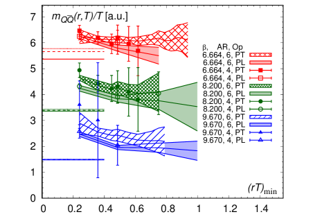
We show the local screening mass from in Fig. 32. There is fair numerical agreement between the screening masses for both aspect ratios. For the smaller volume, we fail to determine reliably for the highest temperature, which is caused by the much smaller signal and, thus, the much worse signal-to-noise ratio. At lower temperatures, the agreement between for different volumes is quite remarkable, in particular, the screening mass assumes a plateau already at , which is approached from above. We observe that the difference between for and for is about 0.5. We use this difference to correct for screening masses determined at on lattices with aspect ratio and assign a systematic uncertainty of to the corrected result. We show the corrected results in Fig. 15, where we include the results for aspect ratio directly at as large open symbols. The screening mass is actually slightly above 2 times the perturbative Debye mass at NLO [Eq. (25)], indicated by the horizontal lines in the lower left corner for the scales , and . We recall that in Fig. 15 we compare with 2 times the NLO Debye mass times a factor . This indicates that for we cannot clearly distinguish between the electrostatic and the asymptotic screening regimes numerically.
In order to test whether we have already reached the asymptotic behavior, we also include plane-averaged Polyakov loop correlators in the analysis,
| (50) |
where the Polyakov loops are integrated over the plane. Since the operators are separated only in the direction we have and in this case. Since the integration is only two-dimensional the plane-averaged Polyakov loop correlator behaves as
| (51) |
in the regime of asymptotic screening, where is a constant that diverges in the continuum limit. We did not subtract the asymptotic constant along the MD time history, as we found that it is not very helpful given numerical fluctuations in the large distance tail. Using the same approach as discussed for the point-to-point Polyakov loop correlation functions, we determine the screening mass from the plane-averaged Polyakov loop correlation function. Results for both operators are fairly consistent, although the plane-averaged correlator yields for small separations at low temperatures a systematically higher and at high temperatures a systematically lower screening mass by a few percent. These differences are of similar size as the errors in the smaller volume, as the difference between determinations in different volumes, and as well as our correction for the screening mass obtained at [cf. the discussion preceding Eq. (50)]. Therefore, we consider the screening masses as consistent and asymptotic for .
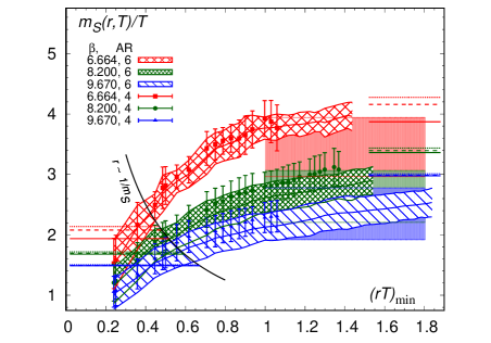
We show the local screening mass from in Fig. 33. Fits with Eq. (49) as Ansatz yield and for . Both outcomes are consistent with the observation in Sec. IV.1 that screening is partially compensated by other medium effects at short distances. For larger we always obtain . for 0.3–0.6 is within errors fairly consistent with the perturbative Debye mass at NLO as indicated by the three horizontal lines in the lower left corner of the figure representing for the scales and . Deviations can be attributed to the higher order terms discussed in Sec. IV.2, which are missing in Eq. (49). There is good numerical agreement between the screening masses for both volumes for . Even in the larger volume, we do not see an unambiguous plateau in for any of the temperatures, although is within errors consistent with a constant for . For this reason, we consider as the asymptotic regime, although the onset of the asymptotic behavior seems to occur already somewhat earlier for lower temperatures. For ensembles with poorer signal-to-noise ratio or low temperatures (), the fits may fail well before and we cannot determine in the asymptotic regime. As for the case of the , we estimate a correction to the screening mass determined at shorter distances. We observe that the difference between determined for and is about 0.75. We use this difference to correct for screening masses determined at on lattices with aspect ratio and assign a systematic uncertainty of to the corrected result. The corrected results are shown as the solid bands in Fig. 33 and appear to underestimate the actual asymptotic screening mass somewhat at low temperatures, . The screening masses in Fig. 14 are obtained with this procedure. We include the results for aspect ratio directly at as large open symbols. We consider this estimate of the asymptotic screening mass as sufficiently accurate for .
References
- Bazavov (2015) Alexei Bazavov, “Lattice QCD at Non-Zero Temperature,” Proceedings, 32nd International Symposium on Lattice Field Theory (Lattice 2014): Brookhaven, NY, USA, June 23-28, 2014, PoS LATTICE2014, 392 (2015).
- Petreczky (2012) P. Petreczky, “Lattice QCD at non-zero temperature,” J. Phys. G39, 093002 (2012), arXiv:1203.5320 [hep-lat] .
- Ding et al. (2015a) Heng-Tong Ding, Frithjof Karsch, and Swagato Mukherjee, “Thermodynamics of strong-interaction matter from Lattice QCD,” Int. J. Mod. Phys. E24, 1530007 (2015a), arXiv:1504.05274 [hep-lat] .
- McLerran and Svetitsky (1981) Larry D. McLerran and Benjamin Svetitsky, “Quark Liberation at High Temperature: A Monte Carlo Study of SU(2) Gauge Theory,” Phys. Rev. D24, 450 (1981).
- Kuti et al. (1981) J. Kuti, J. Polonyi, and K. Szlachanyi, “Monte Carlo Study of SU(2) Gauge Theory at Finite Temperature,” In *Bielefeld 1980, Proceedings, Statistical Mechanics Of Quarks and Hadrons*, 157-170, In *Rebbi, C. ( Ed.): Lattice Gauge Theories and Monte Carlo Simulations*, 287-204. ( Phys. Lett. B98 (1981) 199-204) and Budapest Cent. Res. Inst. Phys. - KFKI-80-067 (80,REC.SEP.) 16 P. (010502) (SEE BOOK INDEX), Phys. Lett. B98, 199 (1981).
- Bazavov et al. (2009) A. Bazavov et al., “Equation of state and QCD transition at finite temperature,” Phys. Rev. D80, 014504 (2009), arXiv:0903.4379 [hep-lat] .
- Bazavov et al. (2012) A. Bazavov et al., “The chiral and deconfinement aspects of the QCD transition,” Phys. Rev. D85, 054503 (2012), arXiv:1111.1710 [hep-lat] .
- Kaczmarek et al. (2002) O. Kaczmarek, F. Karsch, P. Petreczky, and F. Zantow, “Heavy quark anti-quark free energy and the renormalized Polyakov loop,” Phys. Lett. B543, 41–47 (2002), arXiv:hep-lat/0207002 [hep-lat] .
- Bazavov et al. (2016) A. Bazavov, N. Brambilla, H. T. Ding, P. Petreczky, H. P. Schadler, A. Vairo, and J. H. Weber, “Polyakov loop in 2+1 flavor QCD from low to high temperatures,” Phys. Rev. D93, 114502 (2016), arXiv:1603.06637 [hep-lat] .
- Irback et al. (1991) A. Irback, P. LaCock, D. Miller, B. Petersson, and T. Reisz, “The Heavy quark potential in SU(2) gauge theory at high temperature,” Nucl. Phys. B363, 34–64 (1991).
- LaCock et al. (1992) Pierre LaCock, David E. Miller, and Thomas Reisz, “Dimensional reduction of SU(2) gauge theory beyond the perturbative horizon,” Nucl. Phys. B369, 501–518 (1992).
- Datta and Gupta (2000) Saumen Datta and Sourendu Gupta, “Screening masses in SU(2) pure gauge theory,” Phys. Lett. B471, 382–387 (2000), arXiv:hep-lat/9906023 [hep-lat] .
- Fiore et al. (2003) R. Fiore, A. Papa, and P. Provero, “The Spectrum of screening masses near T(c): Predictions from universality,” Phys. Rev. D67, 114508 (2003), arXiv:hep-lat/0302004 [hep-lat] .
- Digal et al. (2003) S. Digal, S. Fortunato, and P. Petreczky, “Heavy quark free energies and screening in SU(2) gauge theory,” Phys. Rev. D68, 034008 (2003), arXiv:hep-lat/0304017 [hep-lat] .
- Bazavov et al. (2008) A. Bazavov, P. Petreczky, and A. Velytsky, “Static quark anti-quark pair in SU(2) gauge theory,” Phys. Rev. D78, 114026 (2008), arXiv:0809.2062 [hep-lat] .
- Karkkainen et al. (1992) Leo Karkkainen, P. Lacock, D. E. Miller, B. Petersson, and T. Reisz, “Dimensional reduction in SU(3) gauge theory,” Phys. Lett. B282, 121–126 (1992).
- Kaczmarek et al. (2000) Olaf Kaczmarek, Frithjof Karsch, Edwin Laermann, and Martin Lutgemeier, “Heavy quark potentials in quenched QCD at high temperature,” Phys. Rev. D62, 034021 (2000), arXiv:hep-lat/9908010 [hep-lat] .
- Petreczky et al. (2002) P. Petreczky, O. Kaczmarek, F. Karsch, E. Laermann, S. Stickan, I. Wetzorke, and F. Zantow, “Lattice calculation of medium effects at short and long distances,” Nucl. Phys. A698, 400–403 (2002), arXiv:hep-lat/0103034 [hep-lat] .
- Akerlund and de Forcrand (2014) Oscar Akerlund and Philippe de Forcrand, “Scale hierarchy in high-temperature QCD,” Proceedings, 31st International Symposium on Lattice Field Theory (Lattice 2013): Mainz, Germany, July 29-August 3, 2013, PoS LATTICE2013, 144 (2014), arXiv:1312.1543 [hep-lat] .
- Detar et al. (1999) Carleton E. Detar, Olaf Kaczmarek, Frithjof Karsch, and Edwin Laermann, “String breaking in lattice quantum chromodynamics,” Phys. Rev. D59, 031501 (1999), arXiv:hep-lat/9808028 [hep-lat] .
- Karsch et al. (2001) F. Karsch, E. Laermann, and A. Peikert, “Quark mass and flavor dependence of the QCD phase transition,” Nucl. Phys. B605, 579–599 (2001), arXiv:hep-lat/0012023 [hep-lat] .
- Kaczmarek and Zantow (2005) Olaf Kaczmarek and Felix Zantow, “Static quark anti-quark interactions in zero and finite temperature QCD. I. Heavy quark free energies, running coupling and quarkonium binding,” Phys. Rev. D71, 114510 (2005), arXiv:hep-lat/0503017 [hep-lat] .
- Petreczky and Petrov (2004) P. Petreczky and K. Petrov, “Free energy of a static quark anti-quark pair and the renormalized Polyakov loop in three flavor QCD,” Phys. Rev. D70, 054503 (2004), arXiv:hep-lat/0405009 [hep-lat] .
- Petreczky (2010) Peter Petreczky, “Quarkonium in Hot Medium,” J. Phys. G37, 094009 (2010), arXiv:1001.5284 [hep-ph] .
- Bazavov and Petreczky (2013a) A. Bazavov and P. Petreczky, “Static quark correlators and quarkonium properties at non-zero temperature,” Proceedings, Extreme QCD 2012 (XQCD12): Washington, USA, August 21-23, 2012, J. Phys. Conf. Ser. 432, 012003 (2013a), arXiv:1211.5638 [hep-lat] .
- Borsanyi, Szabolcs and Fodor, Zoltan and Katz, Sándor D. and Pásztor, Attila and Szabó, Kálmán K. and Török, Csaba (2015) Borsanyi, Szabolcs and Fodor, Zoltan and Katz, Sándor D. and Pásztor, Attila and Szabó, Kálmán K. and Török, Csaba, “Static pair free energy and screening masses from correlators of Polyakov loops: continuum extrapolated lattice results at the QCD physical point,” JHEP 04, 138 (2015), arXiv:1501.02173 [hep-lat] .
- Andreoli et al. (2018) Michele Andreoli, Claudio Bonati, Massimo D’Elia, Michele Mesiti, Francesco Negro, Andrea Rucci, and Francesco Sanfilippo, “Gauge-invariant screening masses and static quark free energies in QCD at nonzero baryon density,” Phys. Rev. D97, 054515 (2018), arXiv:1712.09996 [hep-lat] .
- Gross et al. (1981) David J. Gross, Robert D. Pisarski, and Laurence G. Yaffe, “QCD and Instantons at Finite Temperature,” Rev. Mod. Phys. 53, 43 (1981).
- Nadkarni (1986) Sudhir Nadkarni, “Nonabelian Debye Screening. 1. The Color Averaged Potential,” Phys. Rev. D33, 3738 (1986).
- Brambilla et al. (2010) Nora Brambilla, Jacopo Ghiglieri, Peter Petreczky, and Antonio Vairo, “The Polyakov loop and correlator of Polyakov loops at next-to-next-to-leading order,” Phys. Rev. D82, 074019 (2010), arXiv:1007.5172 [hep-ph] .
- Berwein et al. (2017) Matthias Berwein, Nora Brambilla, Peter Petreczky, and Antonio Vairo, “Polyakov loop correlator in perturbation theory,” Phys. Rev. D96, 014025 (2017), arXiv:1704.07266 [hep-ph] .
- Pineda and Soto (1998) A. Pineda and J. Soto, “Effective field theory for ultrasoft momenta in NRQCD and NRQED,” Quantum chromodynamics. Proceedings, Conference, QCD’97, Montpellier, France, July 3-9, 1997, Nucl. Phys. Proc. Suppl. 64, 428–432 (1998), [,428(1997)], arXiv:hep-ph/9707481 [hep-ph] .
- Brambilla et al. (2000) Nora Brambilla, Antonio Pineda, Joan Soto, and Antonio Vairo, “Potential NRQCD: An Effective theory for heavy quarkonium,” Nucl. Phys. B566, 275 (2000), arXiv:hep-ph/9907240 [hep-ph] .
- Brambilla et al. (2005) Nora Brambilla, Antonio Pineda, Joan Soto, and Antonio Vairo, “Effective field theories for heavy quarkonium,” Rev. Mod. Phys. 77, 1423 (2005), arXiv:hep-ph/0410047 [hep-ph] .
- Braaten and Nieto (1996) Eric Braaten and Agustin Nieto, “Free energy of QCD at high temperature,” Phys. Rev. D53, 3421–3437 (1996), arXiv:hep-ph/9510408 [hep-ph] .
- Linde (1980) Andrei D. Linde, “Infrared Problem in Thermodynamics of the Yang-Mills Gas,” Phys. Lett. B96, 289 (1980).
- Rebhan (1994) Anton K. Rebhan, “NonAbelian Debye screening in one loop resummed perturbation theory,” Nucl. Phys. B430, 319–344 (1994), arXiv:hep-ph/9408262 [hep-ph] .
- Braaten and Nieto (1994) Eric Braaten and Agustin Nieto, “Next-to-leading order Debye mass for the quark - gluon plasma,” Phys. Rev. Lett. 73, 2402–2404 (1994), arXiv:hep-ph/9408273 [hep-ph] .
- Braaten and Nieto (1995) Eric Braaten and Agustin Nieto, “Asymptotic behavior of the correlator for Polyakov loops,” Phys. Rev. Lett. 74, 3530–3533 (1995), arXiv:hep-ph/9410218 [hep-ph] .
- Arnold and Yaffe (1995) Peter Brockway Arnold and Laurence G. Yaffe, “The NonAbelian Debye screening length beyond leading order,” Phys. Rev. D52, 7208–7219 (1995), arXiv:hep-ph/9508280 [hep-ph] .
- Laine and Vepsalainen (2009) M. Laine and M. Vepsalainen, “On the smallest screening masses in hot QCD,” JHEP 09, 023 (2009), arXiv:0906.4450 [hep-ph] .
- Burnier et al. (2010) Y. Burnier, M. Laine, and M. Vepsalainen, “Dimensionally regularized Polyakov loop correlators in hot QCD,” JHEP 01, 054 (2010), [Erratum: JHEP 01, 180 (2013)], arXiv:0911.3480 [hep-ph] .
- Mocsy et al. (2013) Agnes Mocsy, Peter Petreczky, and Michael Strickland, “Quarkonia in the Quark Gluon Plasma,” Int. J. Mod. Phys. A28, 1340012 (2013), arXiv:1302.2180 [hep-ph] .
- Blaizot and Escobedo (2017) Jean-Paul Blaizot and Miguel Angel Escobedo, “Quantum and Classical Dynamics of Heavy Quarks in a Quark-Gluon Plasma,” (2017), arXiv:1711.10812 [hep-ph] .
- Wetzorke et al. (2002) I. Wetzorke, F. Karsch, E. Laermann, P. Petreczky, and S. Stickan, “Meson spectral functions at finite temperature,” Lattice field theory. Proceedings, 19th International Symposium, Lattice 2001, Berlin, Germany, August 19-24, 2001, Nucl. Phys. Proc. Suppl. 106, 510–512 (2002), arXiv:hep-lat/0110132 [hep-lat] .
- Datta et al. (2004) Saumen Datta, Frithjof Karsch, Peter Petreczky, and Ines Wetzorke, “Behavior of charmonium systems after deconfinement,” Phys. Rev. D69, 094507 (2004), arXiv:hep-lat/0312037 [hep-lat] .
- Burnier et al. (2008) Y. Burnier, M. Laine, and M. Vepsalainen, “Heavy quarkonium in any channel in resummed hot QCD,” JHEP 01, 043 (2008), arXiv:0711.1743 [hep-ph] .
- Brambilla et al. (2008) Nora Brambilla, Jacopo Ghiglieri, Antonio Vairo, and Peter Petreczky, “Static quark-antiquark pairs at finite temperature,” Phys. Rev. D78, 014017 (2008), arXiv:0804.0993 [hep-ph] .
- Petreczky et al. (2011) Peter Petreczky, Chuan Miao, and Agnes Mocsy, “Quarkonium spectral functions with complex potential,” Nucl. Phys. A855, 125–132 (2011), arXiv:1012.4433 [hep-ph] .
- Burnier et al. (2015) Yannis Burnier, Olaf Kaczmarek, and Alexander Rothkopf, “Quarkonium at finite temperature: Towards realistic phenomenology from first principles,” JHEP 12, 101 (2015), arXiv:1509.07366 [hep-ph] .
- Burnier et al. (2016) Yannis Burnier, Olaf Kaczmarek, and Alexander Rothkopf, “In-medium P-wave quarkonium from the complex lattice QCD potential,” JHEP 10, 032 (2016), arXiv:1606.06211 [hep-ph] .
- Brambilla et al. (2017) Nora Brambilla, Miguel A. Escobedo, Joan Soto, and Antonio Vairo, “Quarkonium suppression in heavy-ion collisions: an open quantum system approach,” Phys. Rev. D96, 034021 (2017), arXiv:1612.07248 [hep-ph] .
- Brambilla et al. (2018) Nora Brambilla, Miguel A. Escobedo, Joan Soto, and Antonio Vairo, “Heavy quarkonium suppression in a fireball,” Phys. Rev. D97, 074009 (2018), arXiv:1711.04515 [hep-ph] .
- Weber et al. (2016) Johannes Heinrich Weber, Peter Petreczky, and Alexei Bazavov, “Polyakov loop correlators and cyclic Wilson loop from lattice QCD,” Proceedings, 33rd International Symposium on Lattice Field Theory (Lattice 2015): Kobe, Japan, July 14-18, 2015, PoS LATTICE2015, 177 (2016), arXiv:1601.08001 [hep-lat] .
- Petreczky and Weber (2016) Peter Petreczky and Johannes Weber, “Deconfinement and color screening in 2+1 flavor QCD,” EPJ Web Conf. 120, 07001 (2016).
- Weber (2017) Johannes Heinrich Weber (TUMQCD), “Lattice calculation of the Polyakov loop and Polyakov loop correlators,” Proceedings, 12th Conference on Quark Confinement and the Hadron Spectrum (Confinement XII): Thessaloniki, Greece, EPJ Web Conf. 137, 07028 (2017).
- Follana et al. (2007) E. Follana, Q. Mason, C. Davies, K. Hornbostel, G. P. Lepage, J. Shigemitsu, H. Trottier, and K. Wong (HPQCD, UKQCD), “Highly improved staggered quarks on the lattice, with applications to charm physics,” Phys. Rev. D75, 054502 (2007), arXiv:hep-lat/0610092 [hep-lat] .
- Bazavov et al. (2014a) A. Bazavov et al. (HotQCD), “Equation of state in ( 2+1 )-flavor QCD,” Phys. Rev. D90, 094503 (2014a), arXiv:1407.6387 [hep-lat] .
- Ding et al. (2015b) H. T. Ding, Swagato Mukherjee, H. Ohno, P. Petreczky, and H. P. Schadler, “Diagonal and off-diagonal quark number susceptibilities at high temperatures,” Phys. Rev. D92, 074043 (2015b), arXiv:1507.06637 [hep-lat] .
- Bazavov et al. (2013) A. Bazavov, H. T. Ding, P. Hegde, F. Karsch, C. Miao, Swagato Mukherjee, P. Petreczky, C. Schmidt, and A. Velytsky, “Quark number susceptibilities at high temperatures,” Phys. Rev. D88, 094021 (2013), arXiv:1309.2317 [hep-lat] .
- Bazavov and Petreczky (2013b) A. Bazavov and P. Petreczky, “Polyakov loop in 2+1 flavor QCD,” Phys.Rev. D87, 094505 (2013b), arXiv:1301.3943 [hep-lat] .
- Bazavov et al. (2010) A. Bazavov et al. (MILC), “Scaling studies of QCD with the dynamical HISQ action,” Phys. Rev. D82, 074501 (2010), arXiv:1004.0342 [hep-lat] .
- Jahn and Philipsen (2004) Oliver Jahn and Owe Philipsen, “The Polyakov loop and its relation to static quark potentials and free energies,” Phys. Rev. D70, 074504 (2004), arXiv:hep-lat/0407042 [hep-lat] .
- Berwein et al. (2013) Matthias Berwein, Nora Brambilla, Jacopo Ghiglieri, and Antonio Vairo, “Renormalization of the cyclic Wilson loop,” JHEP 03, 069 (2013), arXiv:1212.4413 [hep-th] .
- Bazavov and Petreczky (2013c) A. Bazavov and P. Petreczky, “Static meson correlators in 2+1 flavor QCD at non-zero temperature,” Eur. Phys. J. A49, 85 (2013c), arXiv:1303.5500 [hep-lat] .
- Berwein et al. (2014) Matthias Berwein, Nora Brambilla, and Antonio Vairo, “Renormalization of Loop Functions in QCD,” Phys. Part. Nucl. 45, 656–663 (2014), arXiv:1312.6651 [hep-th] .
- Hasenfratz and Knechtli (2001) Anna Hasenfratz and Francesco Knechtli, “Flavor symmetry and the static potential with hypercubic blocking,” Phys. Rev. D64, 034504 (2001), arXiv:hep-lat/0103029 [hep-lat] .
- Bazavov et al. (2018) A. Bazavov, P. Petreczky, and J. H. Weber, “Equation of State in 2+1 Flavor QCD at High Temperatures,” Phys. Rev. D97, 014510 (2018), arXiv:1710.05024 [hep-lat] .
- Bazavov et al. (2014b) Alexei Bazavov, Nora Brambilla, Xavier Garcia i Tormo, Peter Petreczky, Joan Soto, and Antonio Vairo, “Determination of from the QCD static energy: An update,” Phys. Rev. D90, 074038 (2014b).
- Kaczmarek et al. (2004) O. Kaczmarek, F. Karsch, F. Zantow, and P. Petreczky, “Static quark anti-quark free energy and the running coupling at finite temperature,” Phys. Rev. D70, 074505 (2004), [Erratum: Phys. Rev.D72,059903(2005)], arXiv:hep-lat/0406036 [hep-lat] .
- Brambilla et al. (1999) Nora Brambilla, Antonio Pineda, Joan Soto, and Antonio Vairo, “The Infrared behavior of the static potential in perturbative QCD,” Phys. Rev. D60, 091502 (1999), arXiv:hep-ph/9903355 [hep-ph] .
- Maezawa and Petreczky (2016) Y. Maezawa and P. Petreczky, “Quark masses and strong coupling constant in 2+1 flavor QCD,” Phys. Rev. D94, 034507 (2016), arXiv:1606.08798 [hep-lat] .
- Berwein et al. (2016) Matthias Berwein, Nora Brambilla, Peter Petreczky, and Antonio Vairo, “Polyakov loop at next-to-next-to-leading order,” Phys. Rev. D93, 034010 (2016), arXiv:1512.08443 [hep-ph] .
- Heller et al. (1998) Urs M. Heller, F. Karsch, and J. Rank, “The Gluon propagator at high temperature: Screening, improvement and nonzero momenta,” Phys. Rev. D57, 1438–1448 (1998), arXiv:hep-lat/9710033 [hep-lat] .
- Karsch et al. (1998) F. Karsch, M. Oevers, and P. Petreczky, “Screening masses of hot SU(2) gauge theory from the 3-d adjoint Higgs model,” Phys. Lett. B442, 291–299 (1998), arXiv:hep-lat/9807035 [hep-lat] .
- Petreczky and Schadler (2015) P. Petreczky and H. P. Schadler, “Renormalization of the Polyakov loop with gradient flow,” Phys. Rev. D92, 094517 (2015), arXiv:1509.07874 [hep-lat] .
- Kniehl et al. (2005) B. A. Kniehl, A. A. Penin, Y. Schroder, Vladimir A. Smirnov, and M. Steinhauser, “Two-loop static QCD potential for general colour state,” Phys. Lett. B607, 96–100 (2005), arXiv:hep-ph/0412083 [hep-ph] .
- Kaczmarek (2007) Olaf Kaczmarek, “Screening at finite temperature and density,” Proceedings, 4th International Workshop on Critical point and onset of deconfinement (CPOD07): Darmstadt, Germany, July 9-13, 2007, PoS CPOD07, 043 (2007), arXiv:0710.0498 [hep-lat] .
- Hart et al. (2000) A. Hart, M. Laine, and O. Philipsen, “Static correlation lengths in QCD at high temperatures and finite densities,” Nucl. Phys. B586, 443–474 (2000), arXiv:hep-ph/0004060 [hep-ph] .
- Kajantie et al. (1997) K. Kajantie, M. Laine, K. Rummukainen, and Mikhail E. Shaposhnikov, “3-D SU(N) + adjoint Higgs theory and finite temperature QCD,” Nucl. Phys. B503, 357–384 (1997), arXiv:hep-ph/9704416 [hep-ph] .
- Hart and Philipsen (2000) A. Hart and O. Philipsen, “The Spectrum of the three-dimensional adjoint Higgs model and hot SU(2) gauge theory,” Nucl. Phys. B572, 243–265 (2000), arXiv:hep-lat/9908041 [hep-lat] .
- Bellwied et al. (2015) R. Bellwied, S. Borsanyi, Z. Fodor, S. D. Katz, A. Pasztor, C. Ratti, and K. K. Szabo, “Fluctuations and correlations in high temperature QCD,” Phys. Rev. D92, 114505 (2015), arXiv:1507.04627 [hep-lat] .
- Borsanyi et al. (2016) Sz. Borsanyi et al., “Calculation of the axion mass based on high-temperature lattice quantum chromodynamics,” Nature 539, 69–71 (2016), arXiv:1606.07494 [hep-lat] .
- Petreczky et al. (2016) Peter Petreczky, Hans-Peter Schadler, and Sayantan Sharma, “The topological susceptibility in finite temperature QCD and axion cosmology,” Phys. Lett. B762, 498–505 (2016), arXiv:1606.03145 [hep-lat] .
- Bonati et al. (2016) Claudio Bonati, Massimo D’Elia, Marco Mariti, Guido Martinelli, Michele Mesiti, Francesco Negro, Francesco Sanfilippo, and Giovanni Villadoro, “Axion phenomenology and -dependence from lattice QCD,” JHEP 03, 155 (2016), arXiv:1512.06746 [hep-lat] .
- R Core Team (2018) R Core Team, R: A Language and Environment for Statistical Computing, R Foundation for Statistical Computing, Vienna, Austria (2018).
- Clark et al. (2005) M. A. Clark, A. D. Kennedy, and Z. Sroczynski, “Exact 2+1 flavour RHMC simulations,” Lattice field theory. Proceedings, 22nd International Symposium, Lattice 2004, Batavia, USA, June 21-26, 2004, Nucl. Phys. Proc. Suppl. 140, 835–837 (2005), [,835(2004)], arXiv:hep-lat/0409133 [hep-lat] .
- Pinheiro et al. (2018) Jose Pinheiro, Douglas Bates, Saikat DebRoy, Deepayan Sarkar, and R Core Team, nlme: Linear and Nonlinear Mixed Effects Models (2018), r package version 3.1-137.