Improving timing sensitivity in the microhertz frequency regime: limits from PSR J1713$+$0747 on gravitational waves produced by super-massive black-hole binaries

Abstract

We search for continuous gravitational waves (CGWs) produced by individual super-massive black-hole binaries (SMBHBs) in circular orbits using high-cadence timing observations of PSR J1713$+$0747. We observe this millisecond pulsar using the telescopes in the European Pulsar Timing Array (EPTA) with an average cadence of approximately 1.6 days over the period between April 2011 and July 2015, including an approximately daily average between February 2013 and April 2014. The high-cadence observations are used to improve the pulsar timing sensitivity across the GW frequency range of $0.008-5$ $\upmu$Hz. We use two algorithms in the analysis, including a spectral fitting method and a Bayesian approach. For an independent comparison, we also use a previously published Bayesian algorithm. We find that the Bayesian approaches provide optimal results and the timing observations of the pulsar place a 95 per cent upper limit on the sky-averaged strain amplitude of CGWs to be $\lesssim 3.5\times 10^{-13}$ at a reference frequency of 1 $\upmu$Hz. We also find a 95 per cent upper limit on the sky-averaged strain amplitude of low-frequency CGWs to be $\lesssim 1.4\times 10^{-14}$ at a reference frequency of 20 nHz.

1 Introduction

Millisecond pulsars (MSPs) are old neutron stars that are spun up to periods $\lesssim 30$ ms during a mass accretion phase in binary systems through a so-called recycling process (Radhakrishnan & Srinivasan, 1982; Alpar et al., 1982). They are among the most stable known rotators in the universe and the long-term stability, on a time scale of $>$10 yr, of the rotation of some of them is comparable to that of an atomic clock (e.g. Petit & Tavella, 1996; Hobbs et al., 2012). Due to their high rotational stability, the timing measurements of MSPs can be obtained with a significant accuracy (e.g. Kaspi et al., 1994). Therefore, pulsars have been identified as excellent tools for searching for gravitational waves (GWs) (see Detweiler, 1979; Hellings & Downs, 1983; Jenet et al., 2005).

Pulsar timing is sensitive to low-frequency GWs, from nHz to $\upmu$Hz (see Detweiler, 1979; Hellings & Downs, 1983; Jenet et al., 2005), the natural frequency range of inspiralling SMBHBs. Forming as a consequence of galaxy mergers, SMBHBs are expected to form frequently across cosmic history (e.g. Volonteri et al., 2003). The superposition of GW signals from this cosmic population results in a stochastic gravitational wave background (Rajagopal & Romani, 1995; Jaffe & Backer, 2003; Sesana et al., 2008), although particularly nearby massive systems are likely to result in individually resolvable signals rising above the background level (Sesana et al., 2009). The lower frequency limit of GWs that pulsar timing is sensitive to is $1/T_{\rm obs}$, where $T_{\rm obs}$ is the total observation span, indicating that a longer time-baseline of data helps to probe the low-frequency GWs. The upper frequency limit depends on the data sampling pattern since the observations are not evenly sampled. Most of the previous pulsar-based GW studies have used the traditional averaged Nyquist frequency $N/(2T_{\rm obs})$ as the upper limit, where $N$ is the number of observations (e.g. Yardley et al., 2010; Yi et al., 2014; Zhu et al., 2014; Arzoumanian et al., 2014; Babak et al., 2016). To be consistent with previous studies and compare the results, we restrict our search analysis to the same frequency range. We note that the upper frequency limit for an unevenly sampled data set can be much larger than the averaged Nyquist frequency (see Eyer & Bartholdi, 1999; VanderPlas, 2017), but determining the sensitivity in this frequency range is complicated. In order to probe these low-frequency GWs, high-precision timing of MSPs with sub micro-second timing accuracy is essential. Pulsar Timing Arrays (PTAs) – the European PTA (EPTA; Desvignes et al., 2016), the Parkes PTA (PPTA; Reardon et al., 2016), and the North American Nanohertz Observatory for Gravitational Waves (NANOGrav: Arzoumanian et al., 2015) – provide a unique way to obtain such a high timing accuracy by observing a collection of highly stable MSPs with good cadence over a long-term period. The International PTA (IPTA), a collaboration of the three individual PTAs, observes about 50 MSPs in total with a time baseline range of $\sim(4.5-27)$ yr and an approximately weekly to monthly cadence, including short-term daily observation campaigns (see Verbiest et al., 2016).

The limits on the amplitude, or the strain, of GWs produced by individual SMBHBs have been previously investigated through pulsar timing in several studies (e.g. Lommen & Backer, 2001; Jenet et al., 2004). Babak et al. (2016) used 41 MSPs in the first EPTA data release (Desvignes et al., 2016) and estimated the sky-averaged strain amplitude of CGWs to be in the range of $(0.6-1.5)\times 10^{-14}$ at a frequency of $5-7$ nHz. By using 20 MSPs in the first PPTA data release (Manchester et al., 2013), Zhu et al. (2014) estimated the upper limit on the strain amplitude of CGWs to be $1.7\times 10^{-14}$ at a frequency of 10 nHz. Arzoumanian et al. (2014) used the observations of 17 MSPs reported in Demorest et al. (2013) and placed the upper limit on the strain of CGWs to be $3\times 10^{-14}$ at a frequency of 10 nHz.

Using a spectral fitting method, Yardley et al. (2010) constrained the upper limit on the strain amplitude of CGWs to be about $\sim 1\times 10^{-13}$ at a frequency of $\sim 9$ nHz based on 18 MSPs observed by the PPTA. Following the same method, Yi et al. (2014) estimated the upper limit on the strain amplitude of CGWs based on high-cadence observations of PSR B1937$+$21. They found that the timing of this pulsar constrains an upper limit on the strain amplitude of $\lesssim 1.5\times 10^{-11}$ and $\lesssim 5\times 10^{-14}$ at $10^{-7}$ Hz for random and optimal source location and polarisation of individual GW sources, respectively. In the timing analysis, they noticed an unmodelled periodic noise in the timing residuals (i.e. the difference between the observed and model-predicted time of arrivals of pulses) of PSR B1937$+$21 with an amplitude of 150 ns at a frequency of 3.4 yr^-1. Yi et al. (2014) subtracted this periodic signal by fitting a sinusoid and then used the whitened residuals in the GW search analysis. It has been previously reported in other studies that this pulsar exhibits a high level of red timing noise (see Caballero et al., 2016; Lentati et al., 2016) and a significant dispersion measure (DM) variation (e.g. Kaspi et al., 1994; Manchester et al., 2013; Arzoumanian et al., 2015; Desvignes et al., 2016), where DM accounts for the frequency-dependent time delay of the radio pulses due to electrons in the interstellar medium along the line-of-sight. Therefore, the noise and the DM variation of the pulsar may have perhaps generated this particular periodic signal that was seen in the data. Babak et al. (2016) excluded PSR B1937$+$21 in their GW analysis due to its complicated high-level of timing noise. We note that PSR J1713$+$0747 exhibits a much lower level of timing noise and DM variation across our observation time span (see Desvignes et al., 2016; Arzoumanian et al., 2015). We thus emphasise that PSR J1713$+$0747 is a better choice compared to PSR B1937$+$21 for these types of single-pulsar timing-based GW search analyses. We also note that single-pulsar GW search analyses cannot conclusively detect GWs, rather produce upper limits on strain amplitudes.

PSR J1713$+$0747 is one of the most precisely timed pulsars by PTAs (Desvignes et al., 2016; Reardon et al., 2016; Arzoumanian et al., 2015). It is regularly observed by all the telescopes involved in PTAs, providing a timing stability of $\sim 100$ ns based on the recent NANOGrav data release which contains over 9 years of observations (Arzoumanian et al., 2015). Zhu et al. (2015) reported a timing stability of $\sim 92$ ns based on 21 years of observations of the pulsar. Shannon & Cordes (2012) investigated the stability of the pulsar and reported that single pulses show an rms phase fluctuation (the so-called pulse jitter) of $\sim 40$ ns, which limits the timing precision. Recently, Liu et al. (2016a) analysed the single pulses of the pulsar in detail with data collected by the Large European Array for Pulsars (LEAP – Bassa et al., 2016) project and confirmed that the pulsar shows two modes of systematic sub-pulse drifting (Edwards & Stappers, 2003). The IPTA undertook a 24-hr continuous global observation campaign of this pulsar using nine telescopes around the world (Dolch et al., 2014). Dolch et al. (2016) showed that the data set in this campaign is sensitive to CGWs with a frequency between $0.01-1$ mHz. Following Yardley et al. (2010), Dolch et al. (2016) estimated the upper limit on the strain amplitude of CGWs produced by the sources located in the direction of the pulsar to be $\sim 10^{-11}$ at a frequency $0.01$ mHz.

The high-cadence observations are important to understand the noise, and the GW signal if it is present, in pulsar timing data. Since the observations are unevenly sampled, decreasing the relative cadence of the data will increase the noise level across the power spectrum of the timing residuals. The paper is organised as follows: in Section 2, we present our observations and data processing. We describe the timing analysis of the pulsar in Section 3 and present our timing measurements and residuals. We then present our analysis carried out to obtain the upper limit on the strain amplitude of CGWs in Section 4.1 and 4.2 using a spectral fitting and a Bayesian approach, respectively. For an independent comparison, we use the algorithm described in Babak et al. (2016) on our data set and present the results in Section 4.3. We apply our limits on SMBHB candidates in Section 4.4 and investigate any possibilities of detecting them. Finally in Section 5, we summaries our results.

2 Observations and data processing

PSR J1713$+$0747 was observed using the Lovell Telescope (LT) at the Jodrell Bank Observatory between 2011 April and 2015 July with an average cadence of about $4.5$ days. Between 2013 February and 2014 April, the pulsar was observed more frequently with an average cadence of approximately every two days. All the LT observations were carried out at L-band (with a centre frequency of 1532 MHz) and the data were recorded using the ‘ROACH’ pulsar backend (see Bassa et al., 2016). In addition to these high-cadence LT observations, we included the observations of the pulsar obtained from three other telescopes – Effelsberg Telescope (EFF) in Germany, Nançay Radio Telescope (NRT) in France, and Westerbork Synthesis Radio Telescope (WSRT) in the Netherlands – in the analysis to further improve the cadence. The EFF observations were recorded using the ‘PSRIX’ backend (see Lazarus et al., 2016) and carried out at two centre frequencies, 1347 and 2627 MHz. Both single- and multi-beam L-band receivers were used at EFF alternatively throughout our observation time span. The NRT observations were made at centre frequencies of 1484, 1524 and 2539 MHz using the ‘NUPPI’ backend (see Cognard & Theureau, 2006; Cognard et al., 2013). The WSRT observations in this analysis were recorded using the ‘PuMa II’ backend (see Karuppusamy et al., 2008) and observed at three centre frequencies 350, 1380, and 2200 MHz. All these backends used DSPSR to perform coherent dedispersion and folding (van Straten & Bailes, 2011). We note that these observations were obtained using newer backends and are different from the data sets reported in the EPTA data release (Desvignes et al., 2016). To be consistent with all observations, we selected the beginning and the end time of each data set to be equal to that of the LT observations, but we note that the NRT observations started four months after the beginning of the LT observations. The details of the bandwidths, data span, and the number of observations in each data set is given in Table 1. Combining the data from all four telescopes, 952 observation epochs were included in our analysis with a resulting average cadence of about 1.6 days. We also note that the combination of data from other telescopes improved the average cadence of the pulsar to approximately daily within the period between 2013 February and 2014 April, including 420 TOAs in total, in which it was monitored more frequently using the LT.

Table 1: Details of observations used in the analysis. Two $1.347$ GHz Effelsberg data sets have been included in the analysis; the data obtained using the multi-beam receiver (denoted as ‘^m’) and the single-beam receiver (denoted as ‘^s’). The observation length varies and typical values for data sets are given. In total, 952 observation epochs were included in the analysis, resulting in an average cadence of about 1.6 days. The last column shows EFAC and $\rm\log_{10}[EQUAD(s)]$ determined for each data set in the timing model given in Table 2.

Data set	Backend	Centre Freq	Bandwidth	Channel size	Phase	Obs. length	Data span	No. of	Ef,
		(MHz)	(MHz)	(MHz)	bins	(min)		TOAs	$\rm\log_{10}[E_{\rm q}(s)]$
LT	ROACH	1532	400	1	2048a	10/30/60	4/2011 – 7/2015	336	1.00, $-6.81$
NRT	NUPPI	1484	512	4	2048	42	8/2011 – 7/2015	193	1.23, $-6.98$
		1524	512	16	2048	45	1/2013 – 5/2015	20	1.11, $-7.31$
		2539	512	4	2048	52	8/2011 – 12/2014	37	1.34, $-6.57$
EFF	PSRIX	1347m	200	1.56	1024	28	4/2011 – 5/2015	56	1.25, $-6.59$
		1347s	200	1.56	1024	28	5/2011 – 5/2013	27	1.42, $-6.83$
		2627	200	1.56	1024	30	4/2011 – 6/2015	41	1.06, $-6.22$
WSRT	PuMaII	350	70	0.156	256	25/40/60	4/2011 – 7/2015	87	1.11, $-9.80$
		1380	160	0.312	512	25/45	4/2011 – 7/2015	123	0.97, $-6.47$
		2200	160	0.312	512	25/40	4/2011 – 12/2014	32	0.67, $-7.09$

a Note that there were only 512 pulse phase bins in the early LT observations (i.e. before 2011 July – MJD 55754). Therefore, we fit

for an additional ‘JUMP’ in the timing analysis to correct for the time delay of these TOAs.

We processed the data using the pulsar analysis software package PSRCHIVE (Hotan et al., 2004; van Straten et al., 2012). PSR J1713$+$0747 is well known to show a frequency-dependent pulse profile shape variation (see Dolch et al., 2014; Arzoumanian et al., 2015; Zhu et al., 2015), even within a frequency range of a wide-band receiver ($\sim$400 MHz). This may add an extra uncertainty in the measured time-of-arrival (TOA) if it is obtained through the standard bandwidth-averaged TOA generating method (Taylor, 1992). We also note that the scintillation of the pulsar may lead to significant changes in the bandwidth-averaged pulse profile shape due to attenuation of the intensity of the different parts of the frequency band in different observations. Therefore, we use broad-band TOA measurement techniques (see Pennucci et al., 2014; Liu et al., 2014) on LT and NRT observations. Each epoch was first folded for the entire observation duration using a previously published timing model of the pulsar (Desvignes et al., 2016), while keeping the full frequency resolution across the bandwidth. This gives better signal-to-noise (S/N) in frequency-channel-dependent pulse profiles. We then sum neighbouring frequency channels together to form eight equal width sub-bands to further improve the S/N. We then use the software introduced in Pennucci et al. (2014) along with 2D eight sub-band noise-free templates to generate TOAs. The telescope-dependent 2D templates were created by using the results of the frequency-dependent pulse profile evolution analysis (Perera et al. in preparation) which was based on the high-resolution observations reported in Dolch et al. (2014). We note that these TOAs improved the weighted rms of the timing residuals of LT observations alone by a factor of two compared to that obtained using the standard bandwidth-averaged TOA method (Taylor, 1992).

The EFF and WSRT backends use bandwidths a factor of more than 2 smaller (see Table 1) and, therefore, the frequency-dependent profile variation becomes less significant. Thus, we use the standard technique (Taylor, 1992) for the remaining data.

3 Timing the pulsar

We fit a previously published timing model (Desvignes et al., 2016) to our observed TOAs and update the solution by minimising the chi-square of timing residuals using the pulsar timing software package TEMPO2 (Edwards et al., 2006; Hobbs et al., 2006). Since the pulsar is in a binary orbit, the timing model includes Keplerian and Post-Keplerian (PK) parameters (see Lorimer & Kramer, 2005). We combine TOAs from different telescopes/backends by fitting for time offsets or ‘JUMPs’ in the timing model to account for any systemic delays between the data sets (e.g. Verbiest et al., 2016). Note that some of our observations were obtained simultaneously using all/several telescopes as a part of LEAP observations (Bassa et al., 2016). Therefore, these simultaneous observations further help in constraining the ‘JUMPs’ between the relevant data sets in the timing analysis. We note that the interferometric delay measurements between telescopes were not used for these LEAP observations to correct their relative time offsets. We determine the white noise of the pulsar by using the “TEMPONEST” (Lentati et al., 2014) plugin that is based on a Bayesian analysis. We include white noise parameters EFAC, $E_{f}$, and EQUAD, $E_{q}$, for each telescope/backend separately in our timing model, which are related to a TOA with uncertainty $\sigma_{t}$ in micro-seconds as $\sigma=\sqrt{E_{q}^{2}+E_{F}^{2}\sigma_{t}^{2}}$ (see Lentati et al., 2014; Verbiest et al., 2016). We use uniform and log-uniform prior distributions for EFACs and EQUADs in the fit, respectively. We note that our parallax measurement is barely consistent with those reported in other studies (see Zhu et al., 2015; Desvignes et al., 2016; Verbiest et al., 2016). This could be due to different data lengths used in different analyses (e.g. 4.3 yrs of data in our work compared to 17.7 yrs of data in Desvignes et al. (2016)), or some covariance between parameters. Therefore, we use their parallax of $0.90(3)$ and keep it fixed.

The observing frequencies of our data sets span $\sim$$350-2627$ MHz (see Table 1). This broad frequency range allows us to fit for the ${\rm DM}$ and its first two time derivatives, $\rm\dot{DM}(\equiv dDM/dt)$ and $\rm\ddot{DM}(\equiv d^{2}DM/dt^{2})$, in the timing model, and we measure a $\rm\ddot{DM}$ with a 3.5$\sigma$ significance. The pulsar showed a significant DM event towards the end of 2008 (see Desvignes et al., 2016; Arzoumanian et al., 2015; Zhu et al., 2015). However, the TOAs in our data sets begin in 2011 and therefore, no effect from this event is seen in the analysis and we see no evidence for any subsequent events. The timing residuals shown in Figure 1 are based on the timing model given in Table 2. We note that these results were obtained without including red and stochastic DM noise modelling of the pulsar in the timing analysis.

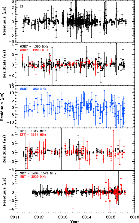
Figure 1: The timing residuals of PSR J1713$+$0747. The weighted rms of the residuals is 219 ns. For clarity of the plot, the residuals of the different telescopes are shown in separate panels. The $\sim$1.4 GHz observations are presented in black, and the low- and high-frequency observations are presented in blue and red colours, respectively. Note that each panel shows different scale in residuals. The average cadence of observations is 1.6 days across the entire data span, while the very-high-cadence observation period between 2013 February and 2014 April achieved an approximately daily observation cadence. Note that the WSRT 350 MHz data set has comparably large uncertainties and thus its weight in the timing analysis is small, although it contributes to the significance of the DM parameters.

Table 2: The timing model parameters of PSR J1713$+$0747 constrained using our data set given in Table 1. The binary parameters were measured using the T2 binary model given in TEMPO2. We keep the parallax fixed at the value $0.90(3)$ reported in Desvignes et al. (2016). The position, spin frequency, and DM are given for the reference epoch of MJD 56000.

Timing parameter
Data span (MJD)	55643 – 57221
Number of TOAs	952
Weighted rms timing residual ($\upmu$s)	0.219
Reduced $\chi^{2}$ value	0.97
Right ascension (RA) (J2000)	17:13:49.5340822(7)
Declination (DEC)(J2000)	$+$07:47:37.48181(2)
Proper motion in RA (mas$/$yr)	4.913(4)
Proper motion in DEC (mas$/$yr)	$-$3.955(8)
Spin frequency, $f$ ($\rm s^{-1}$)	218.8118403818720(3)
Spin frequency $\rm 1^{st}$ time derivative, $\dot{f}$ ($\rm s^{-2}$)	$-4.08356(7)\times 10^{-16}$
Reference epoch (MJD)	56000
Parallax, $\pi$ (mas)	0.9
Dispersion measure, $\rm DM$ (cm-3 pc)	15.99191(4)
Dispersion measure $\rm 1^{st}$ time derivative, $\rm\dot{DM}$(cm-3 pc yr-1)	$-1.0(2)\times 10^{-4}$
Dispersion measure $\rm 2^{nd}$ time derivative, $\rm\ddot{DM}$ (cm-3 pc yr-2)	$2.8(8)\times 10^{-5}$
Orbital period, $P_{\rm b}$ (d)	67.8251309805(6)
Epoch of periastron, $T_{0}$ (MJD)	48741.9740(2)
Projected semi-major axis, $x$ (lt-s)	32.34241993(5)
Longitude of periastron, $\omega$ (deg)	176.201(1)
Orbital eccentricity, $e$	$7.49404(6)\times 10^{-5}$
Orbital inclination, $i$ (deg)	70.4(8)
Longitude of ascending node, $\Omega$ (deg)	96(3)
Companion mass, $m_{c}$ (M⊙)	0.301(3)
Clock correction procedure	TT(BIPM2015)
Solar system ephemeris model	DE421
Units	TCB

The measurements of the two PK parameters, range $r$ and shape $s$, correspond to the Shapiro delay (i.e. the extra time delay of the signal due to the gravitational potential of the binary companion), which leads to measurements of the mass of the pulsar $m_{\rm p}=1.41(6)$ M_⊙ and the companion $m_{\rm c}=0.301(8)$ M_⊙ with a 2$\sigma$ uncertainty. We find that these measurements are consistent with the values reported in previous studies within their uncertainties (see Zhu et al., 2015; Desvignes et al., 2016; Verbiest et al., 2016).

PSR J1713$+$0747 exhibits some low-level red noise and stochastic DM noise in longer data sets (e.g. Zhu et al., 2015; Caballero et al., 2016; Lentati et al., 2016). The length of our data set is perhaps not long enough to perform a proper noise analysis of the pulsar to measure the appropriate parameters significantly. However, for comparison, we determine the red and DM stochastic noise parameters of the pulsar based on our data set using “TEMPONEST” (see Lee et al., 2014; Lentati et al., 2014). We include a power-law DM to model a stochastic DM variation component in addition to $\rm\dot{DM}$ and $\rm\ddot{DM}$ in the timing model. To model an additional achromatic red noise process, we include a power-law red noise model and fit for all white and red noise terms along with the parameters given in the timing model simultaneously. We find that the timing measurements are consistent with those obtained without including these additional noise parameters in the timing model. We find the amplitude and the spectral index of the power-law DM variation are $\log A_{\rm DM}=-14.4\pm 2.5$ and $\gamma_{\rm DM}=2.3\pm 1.8$, respectively, while those of the power-law red noise of the pulsar are $\log A_{\rm red}=-14.9\pm 1.7$ and $\gamma_{\rm red}=2.0\pm 1.7$, respectively. Note that these noise parameters are poorly constrained due to our short data span, but consistent with those estimated in previous studies for this pulsar within the uncertainties (see Desvignes et al., 2016; Verbiest et al., 2016; Caballero et al., 2016). We estimate the Bayes factor (i.e. $B=evidence[H_{1}]/evidence[H_{0}]$, where H₁ is the model including the red and DM stochastic noise and H₀ is the model excluding these noise terms) to be $\log_{10}({\rm B})=8.8(2)$, indicating that the noise model is preferred (Kass & Raftery, 1995).

Note that we use the solar system ephemeris DE421 model (Folkner et al., 2009) in our timing analysis (see Table 2). For an additional comparison, we use the more recent DE436 model in the timing analysis and confirm that the timing and noise parameters are very similar to those obtained with the DE421 model. We also confirm that the GW search results that obtained from the two models are similar and consistent with each other.

4 Pulsar sensitivity to individual gravitational wave sources

The GW signal produced by a SMBHB can be seen in the pulsar timing residuals if the pulsar has a sufficiently precise timing solution and the strain amplitude of the particular GW is large enough to produce a detectable signal in the timing residuals that can be distinguished from the timing noise. The sinusoidal GW signature in timing residuals produced by a SMBHB in a circular orbit has two terms due to its binary evolution, namely the ‘Earth term’, which has a high-frequency behaviour, and the ‘pulsar term’, which has a low-frequency behaviour (see Jenet et al., 2004). We use the GW model given in Babak et al. (2016), and briefly describe the relevant expressions here in Appendix A. In this study, we mainly assume non-evolving SMBHBs (i.e. the long-term evolution of the binary is negligible compared to the light travel time between the pulsar and the Earth), so that both the pulsar and Earth terms have the same frequency. We note that the sources might or might not be evolving at the high frequencies relevant to this study depending on the mass of the SMBHB. However, Babak et al. (2016) showed that the GW upper limits are insensitive on the assumed source model (as we will also confirm this in Section 4.3), which indicates this working assumption is valid. By searching for the embedded GW periodic signal in timing residuals, we would be able to estimate the sensitivity limit of the pulsar on the strain amplitude of the CGWs produced by SMBHBs. We followed two different methods. First, we used computationally inexpensive spectral fitting method given in Yardley et al. (2010). We then undertook a computationally expensive more advanced Bayesian approach using the “TEMPONEST” plugin in TEMPO2. For an independent comparison, we finally use a previously developed algorithm for the first EPTA data release based on Bayesian analysis (Babak et al., 2016), including evolving SMBHBs. We find both Bayesian analyses give consistent upper limits on the strain amplitude, while the spectral method does not provide optimal results, rather it provides slightly larger upper limits. As discussed in Ellis et al. (2012), this spectral fitting method is incoherent and thus, provides non-optimal results. For completeness, we first discuss the spectral fitting method and then the Bayesian approaches.

4.1 Spectral fitting method

As mentioned before, here we use the spectral fitting method given in Yardley et al. (2010). The definition of the GW signal given in Yardley et al. (2010) (see Equation 4 therein) represents a reduced form and thus, misses some parameters (e.g. orbital inclination $i$, initial phase $\phi_{0}$ of the GW signal) compared to the full expression given in Appendix A. We notice that, this reduced form provides a few factors poor results in the upper limit estimates. Therefore, we use the full GW expression.

We first obtain the power spectrum of the timing residuals of PSR J1713$+$0747 shown in Figure 1. The power spectrum of an unevenly sampled data set can be obtained by using the Lomb-Scargle periodogram (Lomb, 1976; Scargle, 1982). However, the original LS periodogram does not account for the uncertainties of the data. When generating the power spectrum from timing residuals, it is important to include the uncertainties to avoid any biases of the power in the spectrum to less-weighted residuals. Therefore, we use the Generalised Lomb-Scargle periodogram (GLSP) formalism introduced in Zechmeister & Kürster (2009), which accounts for the uncertainties of the data points by including weights and also fits for a floating-mean. The power spectrum of our timing residuals is given in Figure 2. We note that since the periodogram is weighted by the uncertainties, the low-frequency WSRT 350 MHz residuals with large uncertainties (see Figure 1) do not contribute significantly. This can be clearly seen in the top panel in Figure 2, where the spectrum is calculated including (solid curve) and excluding (dotted curve) the WSRT 350 MHz data, respectively. Note that we shifted the dotted curve down by a factor of 0.1 for clarity of the figure.

Figure 2: The power spectrum of the timing residuals of the pulsar given in Figure 1. The top panel shows the spectrum generated using the entire data set across the full data span, including (solid curve) and excluding (dotted curve) the low frequency WSRT 350 MHz data set. For the clarity of the plot, we shifted the dotted curve down by a factor of 0.1. We note that both curves are very similar, indicating that the GLSP method accounts for the less weighted WSRT 350 MHz data correctly in the periodogram. The middle panel represents the power spectrum generated using the timing residuals after subtracting the wave forms of the red and stochastic DM power-law noise terms as described in Section 3. The bottom panel shows the spectrum for the very-high-cadence period of the observations after accounting for all noise parameters in the timing model. Note that the upper bound of the frequency range is extended beyond 3.5 $\mu$s with this very-high-cadence observations. The y-axis represents the normalised power (see Zechmeister & Kürster, 2009, for details). The vertical dashed and dashed-dotted lines represent the frequencies of 1 yr^-1 and the orbital period of 67.8 d of the pulsar, respectively.

In contrast to PSR B1937$+$21 (see Yi et al., 2014), Figure 2 shows that the timing residuals of PSR J1713$+$0747 do not present any significant unmodelled periodic signals. However, as mentioned in Section 3, we also estimated DM stochastic and red noise parameters in the timing analysis. For comparison, the middle panel in Figure 2 shows the power spectrum after subtracting the time-domain waveforms of these noise terms in the timing model, resulting in a slightly lower spectral power at low-frequencies compared to the previous case. The power spectrum of the residuals, after subtracting the wave forms of additional DM and red noise terms, on the data within the very high-cadence observing period is shown in the bottom panel of Figure 2. No noticeable red noise is seen within this short, but high-cadence, time span. The significant power drop at the yearly period (i.e. a frequency of $\sim 3\times 10^{-8}$ Hz) in Figure 2 is common for all three cases and it is due to fitting for the pulsar position in the timing model. Similarly, the power absorption at $\sim 1.7\times 10^{-7}$ Hz is due to fitting for the orbital period, $P_{\rm b}=67.8$ d.

We then use the same method outlined in previous studies (see Yardley et al., 2010; Yi et al., 2014) to build the detection threshold using the power spectrum of timing residuals. To remove any spurious effects from any apparent unmodelled signals and noise in the timing residuals, we smooth the spectrum given in Figure 2 (top panel) and fit a polynomial. We find that a third-order polynomial function is sufficient to fit the data. We then scale this polynomial by a factor $\alpha$ in power in the spectrum. It is determined by simulating $10^{4}$ data sets with TOAs having uncertainties of 100 ns and cadence that matches the observed data. We then obtain the power spectrum of each realisation and calculate the mean power. We label the mean power of the $i$th spectrum as $m_{\rm i}$. We increase $\alpha$ starting from 1 and count the number of power spectra that have any power value greater than $\alpha m_{\rm i}$. We set a 1% false alarm rate and increase $\alpha$ until the number of spectra satisfies this threshold. We find that the best $\alpha$ for our data set is 10.1, and scale the polynomial in power accordingly, in order to build the detection threshold.

We then divide the frequency range of the observed spectrum into 100 equal bins in log-space. We inject the pulsar and Earth terms at the same frequency, according to the model given in Appendix A, for a given $h_{s}$ in the observed TOAs (see Equation 1). We fit our timing model of the pulsar to the new GW-injected TOAs using TEMPO2 and obtain timing residuals. The power spectrum of the timing residuals is then compared with the detection threshold at the given frequency for a detection (see Yardley et al., 2010; Yi et al., 2014, for more details). For each $h_{s}$, we perform 1000 trials using randomly selected $\phi_{S}$, $\theta_{S}$, $\phi_{0}$, $\psi$, and $i$ and then count the number of detections (see Appendix A for definitions of these parameters). We increase $h_{s}$ until the signals of 95 per cent of trials are detected and then record the particular $h_{s}$ as the upper limit for that given frequency bin. We repeat this process for all frequency bins. This gives the 95 per cent upper limit on the sky-averaged strain amplitude of CGWs produced by SMBHBs. We present our upper limit curve in Figure 3 (see panel (a) and (b)). For an optimal sky location, we assume all the SMBHBs are located in the direction of the pulsar ($\pm 10^{\circ}$ in the direction of the pulsar), and repeat the same procedure as before. As shown in the figure, the optimal upper limit is a factor of a few better than the sky-averaged result.

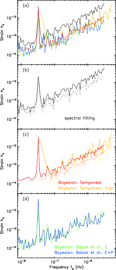
Figure 3: The 95 per cent upper limit on the GW strain amplitude produced by SMBHBs based on the timing observations of PSR J1713$+$0747. Panel (a) shows the results obtained from all methods described in Section 4. For clarity, we plot the results obtained from each method in the following panels (i.e. from spectral fitting, and Bayesian analysis using Temponest and the algorithm given in Babak et al. (2016), respectively). The dotted curves in panel (b) and (c) show the upper limits for the optimal case where all the sources are assumed to be located in the same direction as the pulsar. For comparison, we over plot the upper limits obtained from the data within the high-cadence observation time span between February 2013 and April 2014 (orange curves in panel (c)). Panel (d) shows the upper limits obtained from the algorithm given in Babak et al. (2016) assuming evolving sources, for only the Earth term (green) and also for the combined Earth and pulsar terms (blue).

4.2 Bayesian approach using TEMPONEST

The spectral fitting method described above is an incoherent ad-hoc method that does not provide optimal results. It does not include the noise processes of the pulsar (i.e. red and DM stochastic noise) and it is not straightforward to implement them in the model. If the noise modelling is included in the analysis, then we need to fit for noise properties each time the GW signal is injected and thus, the fitting method becomes computationally inefficient. Therefore, we use the Bayesian approach described in Lentati et al. (2014) where the noise properties of the pulsar are constrained using the “TEMPONEST” plugin. Since we assume that the GW is produced by a SMBHB in a circular orbit, the signal that can be embedded in the data of a single pulsar is sinusoidal. Therefore, we fit for an additional simple sinusoidal signal while fitting for white noise (i.e. EFACs and EQUADs), and power-law stochastic DM and red noise parameters of the pulsar simultaneously using “TEMPONEST”. The timing model parameters are marginalised over during the fit (see Lentati et al., 2014, for details about this procedure). The plugin uses Bayesian inference tool MULTINEST to determine this joint parameter space and nested Markov Chain Monte Carlo method for sampling (Feroz & Hobson, 2008; Feroz et al., 2009; Feroz et al., 2013). We use log-uniform prior distributions for amplitudes of the power-law DM stochastic and red noise, and for the frequency of the sinusoidal signal. We use uniform prior distributions for spectral indices of the power-law noise terms, and the amplitude and the phase of the sinusoidal signal. The fit results in approximately $4\times 10^{4}$ samples in the posterior probability distribution. Each sinusoidal signal sample includes information about its amplitude (r(t)), initial phase ($\phi_{0}$), and the frequency ($f_{g}$). We then convert the amplitudes of these GW signals to strain amplitudes ($h_{s}$) using Equation 1 for randomly selected $\phi_{S}$, $\theta_{S}$, $\phi_{0}$, $\psi$, and $i$ (i.e. the polar coordinates of the GW source, initial phase of the signal, GW polarisation angle, and orbital inclination, respectively – see Appendix A for details). We divide the frequency range of these GWs (which is equal to the frequency range used in Section 4.1) into 100 equal bins and then obtain the 95 per cent upper limit on the strain amplitude of corresponding signals in each bin. Figure 3 shows our results (see panel (a) and (c)). The optimal upper limit is again obtained by considering all sources to be located along the direction of the pulsar (see panel (c) in Figure 3) as described in Section 4.1.

As mentioned above, Figure 3 shows that the Bayesian approach provides better limits compared to the spectral fitting method. We also applied this method to the data within the high-cadence observation time span and obtained the upper limit on the strain amplitude (panel (c) of Figure 3).

4.3 Using previously published Bayesian algorithm

In order to further validate our results, we use the algorithm presented in Babak et al. (2016). In this Bayesian analysis, we use PolyChord (Handley et al., 2015) to fit for the CGW signal (i.e. $h_{s}$, $\phi_{S}$, $\theta_{S}$, $\phi_{0}$, $\psi$, $i$, and $f_{g}$) and the noise parameters (i.e. EFACs, EQUADs, and power-law stochastic DM, and red noise processes). Similar to the method in Section 4.2, the timing model parameters are marginalised over during the fit. In addition to different tools used in the two Bayesian approaches, Babak et al. (2016) is capable of using both evolving and non-evolving sources in the search analysis, whereas the method in Section 4.2 uses only non-evolving sources. The underlying algorithm utilises the GW model described in Appendix A, and the details of the fitting procedure is described in Babak et al. (2016) and Taylor (2017). In the search for evolving sources, we use three extra parameters in the model – the chirp mass of the system, distance to the pulsar, and the initial phase of the pulsar term. For the distance to the pulsar we use the Gaussian prior centred at the best currently known value with the measured uncertainty of 1.05(7) kpc (Chatterjee et al., 2009). As mentioned above, we use PolyChord (nested sampling) in this analysis, which is the next incarnation of the MULTINEST. It is supposed to be more robust for the multi-modal likelihood surfaces embedded in the large dimensional parameter space and more efficient for some problems. However, we find no benefit of the new implementation, rather both samplers give very consistent results. The posterior distribution for the noise parameters obtained by the TEMPONEST (described in the Section 4.2) and the method used here are very similar. We also note that the results obtained from evolving and non-evolving sources are consistent with each other. We present the upper limit on the strain amplitude of CGWs in Figure 3 (see panel (a) and (d)) separately for the Earth term only, as well as for the combined Earth and pulsar terms. Figure 3 shows that these results are consistent with the results obtained from the Bayesian approach described in Section 4.2.

4.4 Application to proposed SMBHB candidates

It is thought that quasars contain SMBHs and SMBHBs in their nuclei. Although SMBHBs are not resolvable optically by direct imaging, candidates can be identified through periodicity in their optical, radio, and X-ray fluxes. The quadrupole torque produced by a binary induces a periodicity in the accretion flow from a circumbinary disk related to its orbital period (Artymowicz & Lubow, 1994; MacFadyen & Milosavljević, 2008; Roedig et al., 2011). This might result in periodic luminosity variations (e.g. Sesana et al., 2012). By searching for periodicities in observations of quasars, SMBHB candidates have been identified in many surveys. In this study we consider those identified by the Catalina Real-time Transient Survey (CRTS) (Graham et al., 2015), Palomar Transient Factory (PTF) data base (Charisi et al., 2016), and Pan-STARRS1 Medium Deep Survey (Liu et al., 2015, 2016b), which identified 111, 33, and 3 candidate SMBHBs, respectively (see Table 3). We note that the periodicities of all these candidate sources are expected to produce GWs in the frequency range between approximately $10^{-8}-10^{-7}$ Hz, which falls into the frequency range that our timing of PSR J1713$+$0747 can probe. Therefore, we estimated these expected signals (using Equation 10 and assuming equal mass SMBHs (i.e. $q=M_{2}/M_{1}=1$) in binary systems) and compared them with our timing derived upper limit on the strain amplitude (see Figure 4). The lower limit of these expected signals shown in the figure are estimated by assuming a mass ratio of $q=M_{2}/M_{1}=0.1$. As seen in Figure 4, the strain amplitudes of the predicted GW signals from these sources are lower (by more than a factor of 4 for the strongest ones) than the sky-averaged sensitivity curve for PSR J1713$+$0747. We note that none of these candidates are located in the direction of the pulsar. Thus, using the actual sky locations of these sources in the GW search analysis will not improve the sensitivity significantly compared to the sky-averaged sensitivity presented in Figure 4 (see the dotted curves in Figure 3 for upper limits based on optimal sky location). This indicates that, we cannot expect to detect GW signals produced by these candidates in our timing results yet.

Table 3: The SMBHB candidates considered in this analysis based on three studies; (1) Catalina Real-time Transient Survey (CRTS) (Graham et al., 2015), (2) Palomar Transient Factory (PTF) data base (Charisi et al., 2016), and (3) Pan-STARRS1 Medium Deep Survey (Liu et al., 2015, 2016b). Note that the expected GW frequencies from these sources fall in the regime that our pulsar timing analysis can be probed.

Study	Candidates	$z$	Period	Frequency
			(yr)	(nHz)
1	111	$0.1-2.7$	$1.8-6.7$	$9.5-35.7$
2	33	$0.3-3.1$	$0.3-2.1$	$29-177$
3	3	$1.2-2.2$	$1.2-1.5$	$41-54$

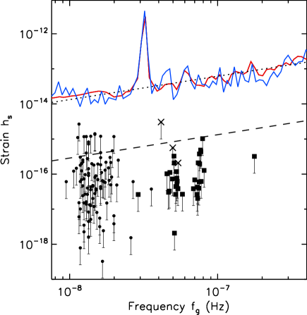
Figure 4: The 95 per cent upper limit on the sky-averaged strain amplitude of CGWs. The colour code of the curves is the same as that given in Figure 3. For clarity, only the limits obtained from Bayesian approaches are plotted. The dashed and dotted lines show the theoretically expected strain amplitude from SMBHBs with equal masses of $10^{9}$ M_⊙ and $10^{8}$ M_⊙ at a distance of the Virgo cluster, 16.5 Mpc, respectively. The circles, squares, and crosses show the expected GW strain amplitude produced by the SMBHB candidates reported in Graham et al. (2015), Charisi et al. (2016), and Liu et al. (2016b), respectively (see Table 3 for more information). Note that the expected strain amplitudes are estimated using Equation 10 given in Appendix A.

5 Conclusions

We used high-cadence observations of PSR J1713$+$0747 to place upper limits on the strain amplitude of CGWs produced by individual SMBHBs in circular orbits. Based on the typical frequency range used in previous studies, $1/T_{\rm obs}$ and $N/(2T_{\rm obs})$ (e.g. Yardley et al., 2010; Yi et al., 2014), we used our observations to probe GWs produced within a frequency range between $7.8\times 10^{-9}$ Hz and $5\times 10^{-6}$ Hz, covering the high-frequency $\upmu$Hz regime. We used three independent methods in the analysis, including a spectral fitting method and more advanced Bayesian approaches. As mentioned in previous studies (see Yardley et al., 2010; Ellis et al., 2012) and also shown in Figure 3, the spectral fitting method does not provide optimal results due to its simple incoherent fitting procedure and absence of proper noise modelling of the pulsar. We find that the independent Bayesian analyses are consistent, and also about a factor of five better compared to the spectral fitting method. Based on our results, we found a 95 per cent upper limit on the sky-averaged strain amplitude of CGWs to be $\lesssim 3.5\times 10^{-13}$ at a reference frequency of $1$ $\upmu$Hz. For an optimal sky location, the 95 per cent upper limit on the strain amplitude is improved to be $\lesssim 2.1\times 10^{-13}$ at the same reference frequency. We also found that our timing results place upper limits on the sky-averaged and optimal strain amplitude of low frequency CGWs to be $\lesssim 1.4\times 10^{-14}$ and $\lesssim 1.1\times 10^{-14}$ at a reference frequency of $20$ nHz, respectively. This low-frequency limit is approximately a three orders of magnitude better compared to the result presented in Yardley et al. (2010) for this pulsar. We also compared our limits with the expected GWs produced by SMBHB candidates, and found that the limits are not yet constraining these sources. However, we will be able to confirm or reject the binary hypothesis for those candidates in the future with better limits including more observations.

Compared to the upper limits of PSR B1937$+$21 on GWs presented in Yi et al. (2014), our study shows that PSR J1713$+$0747 provides better sky-averaged upper limits across the entire frequency range. The poor limits of PSR B1937$+$21 may have been due to excess noise caused by the known significant DM variation and the high-level of red noise in the timing data (see Yi et al., 2014; Caballero et al., 2016; Lentati et al., 2016). As mentioned in Section 4.1, we also note that Yi et al. (2014) used a simplified GW model and it worsens the upper limits by factor of a few compared to that obtained from the full definition of the GW model that we used in our study. The impact of the presence of low-frequency noise in the timing data on their sensitivity to the strain amplitude of GWs was investigated by Caballero et al. (2016) using a subset of the EPTA data over a longer time span of about 17 years. They showed that the sensitivity reduces by a factor of up to $\sim$5 at nHz frequencies while at the higher frequencies that our data set is most sensitive, the impact of noise is minimal.

In comparison, the sensitivity limits on CGWs estimated in our analysis at low-frequencies are consistent in general with those estimated by PTA studies (see Babak et al., 2016; Arzoumanian et al., 2014; Zhu et al., 2014). These PTA studies combined data from several pulsars in their analysis over long-term observations to obtain their sensitivities compared to single-source data over a short-term observations in our analysis. Our study indicates the importance of collecting more high-cadence observations from good pulsars in PTAs to improve the timing precision and then obtain better GW limits even at low-frequencies.

The precision of the timing model (improving the TOA uncertainty) can be improved with time by extending the timing baseline, using larger telescopes and modern backends to observe the pulsar (see Lorimer & Kramer, 2005). Therefore, in the future, we can improve the timing precision by including more data in our analysis and thus, improve the sensitivity limits of pulsar timing to GWs produced by SMBHBs.

Appendix A GW model

The sinusoidal signal produced by a non-evolving GW source in the timing residuals of a pulsar is given by

$$r(t)=r^{e}(t)-r^{p}(t_{p}).$$ (1)

Here, $t_{p}=t-D(1+\hat{\Omega}\cdot\hat{p})/c$, where $D$ is the distance to the pulsar, $c$ is the speed of light, $\hat{\Omega}$ is the unit vector along the direction of GW propagation, and $\hat{p}$ is the unit vector along the direction of the radio waves propagating from the pulsar. We use the astrometry-derived pulsar distance of $1.05(7)$ kpc (Chatterjee et al., 2009), which is consistent with the distance derived from the measured DM and the parallax (see Desvignes et al., 2016). The Earth and pulsar terms are given by

$$\begin{split}r^{e}(t)=&\frac{h_{s}}{\omega}\{(1+\cos^{2}i)F^{+}[\sin(\omega t+\phi_{0})]\\ &+2\cos iF^{\times}[\cos(\omega t+\phi_{0})]\}\end{split}$$ (2)

and

$$\begin{split}r^{p}(t_{p})=&\frac{h_{s}}{\omega}\{(1+\cos^{2}i)F^{+}[\sin(\omega t_{p}+\phi_{0})]\\ &+2\cos iF^{\times}[\cos(\omega t_{p}+\phi_{0})]\}\end{split}$$ (3)

where, $h_{s}$ is the strain amplitude of the GW signal, $f_{g}=\omega/2\pi$ is the frequency of the GW signal, $i$ is the inclination angle of the SMBHB orbit with respect to the line-of-sight, $\phi_{0}$ is the initial phase of the signal. The “antenna beam patterns” are given by

$$F^{+}=\frac{1}{2}\frac{(\hat{m}\cdot\hat{p})^{2}-(\hat{n}\cdot\hat{p})^{2}}{1+\hat{\Omega}\cdot\hat{p}}$$ (4)

and

$$F^{\times}=\frac{(\hat{m}\cdot\hat{p})(\hat{n}\cdot\hat{p})}{1+\hat{\Omega}\cdot\hat{p}}.$$ (5)

For a cartesian coordinate system (x, y, z), we can define all above unit vectors as

$$\begin{split}\hat{m}=&(\sin\phi_{S}\cos\psi-\sin\psi\cos\phi_{S}\cos\theta_{S})\hat{x}\\ &-(\cos\phi_{S}\cos\psi+\sin\psi\sin\phi_{S}\cos\theta_{S})\hat{y}+(\sin\psi\sin\theta_{S})\hat{z}\end{split}$$ (6)

$$\begin{split}\hat{n}=&(-\sin\phi_{S}\sin\psi-\cos\psi\cos\phi_{S}\cos\theta_{S})\hat{x}\\ &+(\cos\phi_{S}\sin\psi-\cos\psi\sin\phi_{S}\cos\theta_{S})\hat{y}+(\cos\psi\sin\theta_{S})\hat{z}\end{split}$$ (7)

$$\hat{\Omega}=-(\sin\theta_{S}\cos\phi_{S})\hat{x}-(\sin\theta_{S}\sin\phi_{S})\hat{y}-\cos\theta_{S}\hat{z}$$ (8)

$$\hat{p}=(\sin\theta\cos\phi)\hat{x}+(\sin\theta\sin\phi)\hat{y}+\cos\theta\hat{z}$$ (9)

where, $\theta_{S}$ and $\phi_{S}$ are the usual polar coordinates of the GW source location in the sky, $\theta$ and $\phi$ are the usual polar coordinates of the pulsar, and $\psi$ is the GW polarisation angle. The derivation of the above expressions are given in previous studies in detail (see Lee et al., 2008; Sesana & Vecchio, 2010; Lee et al., 2011; Zhu et al., 2014; Babak et al., 2016). The GW strain amplitude is defined as

$$h_{s}=2\frac{(GM_{c})^{5/3}}{c^{4}D_{L}(z)}(\pi f_{g})^{2/3}$$ (10)

where, $M_{c}=(M_{1}M_{2})^{3/5}(M_{1}+M_{2})^{-1/5}$ is the chirp mass of the system with individual masses of $M_{1}$ and $M_{2}$, and $G$ is the gravitational constant. The luminosity distance $D_{L}$ to the source is given by

$$D_{L}(z)=(1+z)\frac{c}{H_{0}}\int_{0}^{z}\frac{dz^{\prime}}{E(z^{\prime})},$$ (11)

where, $z$ is the redshift to the source, $H_{0}$ is Hubble’s constant ($=$72 km/s/Mpc), and $E(z)=H(z)/H_{0}=\sqrt{\Omega_{\Lambda}+\Omega_{m}(1+z)^{3}}$ (see Stavridis et al., 2009). We use $\Omega_{\Lambda}=0.7$ and $\Omega_{m}=0.3$ in this work (see Choudhury & Padmanabhan, 2005; Komatsu et al., 2009).

References

- Alpar et al. (1982) Alpar M. A., Cheng A. F., Ruderman M. A., Shaham J., 1982, Nature, 300, 728
- Artymowicz & Lubow (1994) Artymowicz P., Lubow S. H., 1994, ApJ, 421, 651
- Arzoumanian et al. (2014) Arzoumanian Z., et al., 2014, ApJ, 794, 141
- Arzoumanian et al. (2015) Arzoumanian Z., et al., 2015, ApJ, 813, 65
- Babak et al. (2016) Babak S., et al., 2016, MNRAS, 455, 1665
- Bassa et al. (2016) Bassa C. G., et al., 2016, MNRAS, 456, 2196
- Caballero et al. (2016) Caballero R. N., et al., 2016, MNRAS, 457, 4421
- Charisi et al. (2016) Charisi M., Bartos I., Haiman Z., Price-Whelan A. M., Graham M. J., Bellm E. C., Laher R. R., Márka S., 2016, MNRAS, 463, 2145
- Chatterjee et al. (2009) Chatterjee S., et al., 2009, ApJ, 698, 250
- Choudhury & Padmanabhan (2005) Choudhury T. R., Padmanabhan T., 2005, A&A, 429, 807
- Cognard & Theureau (2006) Cognard I., Theureau G., 2006, in IAU Joint Discussion.
- Cognard et al. (2013) Cognard I., Theureau G., Guillemot L., Liu K., Lassus A., Desvignes G., 2013, in Cambresy L., Martins F., Nuss E., Palacios A., eds, SF2A-2013: Proceedings of the Annual meeting of the French Society of Astronomy and Astrophysics. pp 327–330
- Demorest et al. (2013) Demorest P. B., et al., 2013, ApJ, 762, 94
- Desvignes et al. (2016) Desvignes G., et al., 2016, MNRAS, 458, 3341
- Detweiler (1979) Detweiler S., 1979, ApJ, 234, 1100
- Dolch et al. (2014) Dolch T., et al., 2014, ApJ, 794, 21
- Dolch et al. (2016) Dolch T., et al., 2016, Journal of Physics Conference Series, 716, 012014
- Edwards & Stappers (2003) Edwards R. T., Stappers B. W., 2003, A&A, 407, 273
- Edwards et al. (2006) Edwards R. T., Hobbs G. B., Manchester R. N., 2006, MNRAS, 372, 1549
- Ellis et al. (2012) Ellis J. A., Jenet F. A., McLaughlin M. A., 2012, ApJ, 753, 96
- Eyer & Bartholdi (1999) Eyer L., Bartholdi P., 1999, A&AS, 135, 1
- Feroz & Hobson (2008) Feroz F., Hobson M. P., 2008, MNRAS, 384, 449
- Feroz et al. (2009) Feroz F., Hobson M. P., Bridges M., 2009, MNRAS, 398, 1601
- Feroz et al. (2013) Feroz F., Hobson M. P., Cameron E., Pettitt A. N., 2013, preprint, (arXiv:1306.2144)
- Folkner et al. (2009) Folkner W. M., Williams J. G., Boggs D. H., 2009, Interplanetary Network Progress Report, 178, 1
- Graham et al. (2015) Graham M. J., et al., 2015, MNRAS, 453, 1562
- Handley et al. (2015) Handley W. J., Hobson M. P., Lasenby A. N., 2015, MNRAS, 453, 4384
- Hellings & Downs (1983) Hellings R. W., Downs G. S., 1983, ApJ, 265, L39
- Hobbs et al. (2006) Hobbs G. B., Edwards R. T., Manchester R. N., 2006, MNRAS, 369, 655
- Hobbs et al. (2012) Hobbs G., et al., 2012, MNRAS, 427, 2780
- Hotan et al. (2004) Hotan A. W., van Straten W., Manchester R. N., 2004, PASA, 21, 302
- Jaffe & Backer (2003) Jaffe A. H., Backer D. C., 2003, ApJ, 583, 616
- Jenet et al. (2004) Jenet F. A., Lommen A., Larson S. L., Wen L., 2004, ApJ, 606, 799
- Jenet et al. (2005) Jenet F. A., Hobbs G. B., Lee K. J., Manchester R. N., 2005, ApJ, 625, L123
- Karuppusamy et al. (2008) Karuppusamy R., Stappers B., van Straten W., 2008, PASP, 120, 191
- Kaspi et al. (1994) Kaspi V. M., Taylor J. H., Ryba M., 1994, ApJ, 428, 713
- Kass & Raftery (1995) Kass R. E., Raftery A. E., 1995, J. Am. Stat. Assoc, 90, 773
- Komatsu et al. (2009) Komatsu E., et al., 2009, ApJS, 180, 330
- Lazarus et al. (2016) Lazarus P., Karuppusamy R., Graikou E., Caballero R. N., Champion D. J., Lee K. J., Verbiest J. P. W., Kramer M., 2016, MNRAS, 458, 868
- Lee et al. (2008) Lee K. J., Jenet F. A., Price R. H., 2008, ApJ, 685, 1304
- Lee et al. (2011) Lee K. J., Wex N., Kramer M., Stappers B. W., Bassa C. G., Janssen G. H., Karuppusamy R., Smits R., 2011, MNRAS, 414, 3251
- Lee et al. (2014) Lee K. J., et al., 2014, MNRAS, 441, 2831
- Lentati et al. (2014) Lentati L., Alexander P., Hobson M. P., Feroz F., van Haasteren R., Lee K. J., Shannon R. M., 2014, MNRAS, 437, 3004
- Lentati et al. (2016) Lentati L., et al., 2016, MNRAS, 458, 2161
- Liu et al. (2014) Liu K., et al., 2014, MNRAS, 443, 3752
- Liu et al. (2015) Liu T., et al., 2015, ApJ, 803, L16
- Liu et al. (2016a) Liu K., et al., 2016a, MNRAS, 463, 3239
- Liu et al. (2016b) Liu T., et al., 2016b, ApJ, 833, 6
- Lomb (1976) Lomb N. R., 1976, Ap&SS, 39, 447
- Lommen & Backer (2001) Lommen A. N., Backer D. C., 2001, ApJ, 562, 297
- Lorimer & Kramer (2005) Lorimer D. R., Kramer M., 2005, Handbook of Pulsar Astronomy. Cambridge University Press
- MacFadyen & Milosavljević (2008) MacFadyen A. I., Milosavljević M., 2008, ApJ, 672, 83
- Manchester et al. (2013) Manchester R. N., et al., 2013, Publ. Astron. Soc. Australia, 30, e017
- Pennucci et al. (2014) Pennucci T. T., Demorest P. B., Ransom S. M., 2014, ApJ, 790, 93
- Petit & Tavella (1996) Petit G., Tavella P., 1996, A&A, 308, 290
- Radhakrishnan & Srinivasan (1982) Radhakrishnan V., Srinivasan G., 1982, Curr. Sci., 51, 1096
- Rajagopal & Romani (1995) Rajagopal M., Romani R. W., 1995, ApJ, 446, 543
- Reardon et al. (2016) Reardon D. J., et al., 2016, MNRAS, 455, 1751
- Roedig et al. (2011) Roedig C., Dotti M., Sesana A., Cuadra J., Colpi M., 2011, MNRAS, 415, 3033
- Scargle (1982) Scargle J. D., 1982, ApJ, 263, 835
- Sesana & Vecchio (2010) Sesana A., Vecchio A., 2010, Phys. Rev. D, 81, 104008
- Sesana et al. (2008) Sesana A., Vecchio A., Colacino C. N., 2008, MNRAS, 390, 192
- Sesana et al. (2009) Sesana A., Vecchio A., Volonteri M., 2009, MNRAS, 394, 2255
- Sesana et al. (2012) Sesana A., Roedig C., Reynolds M. T., Dotti M., 2012, MNRAS, 420, 860
- Shannon & Cordes (2012) Shannon R. M., Cordes J. M., 2012, ApJ, 761, 64
- Stavridis et al. (2009) Stavridis A., Arun K. G., Will C. M., 2009, Phys. Rev. D, 80, 067501
- Taylor (1992) Taylor J. H., 1992, RSPTA, 341, 117
- Taylor (2017) Taylor S. R., 2017, https://github.com/stevertaylor/NX01, doi:10.5281/zenodo.250258, https://doi.org/10.5281/zenodo.250258
- VanderPlas (2017) VanderPlas J. T., 2017, preprint, (arXiv:1703.09824)
- Verbiest et al. (2016) Verbiest J. P. W., et al., 2016, MNRAS, 458, 1267
- Volonteri et al. (2003) Volonteri M., Haardt F., Madau P., 2003, ApJ, 582, 559
- Yardley et al. (2010) Yardley D. R. B., et al., 2010, MNRAS, 407, 669
- Yi et al. (2014) Yi S., Stappers B. W., Sanidas S. A., Bassa C. G., Janssen G. H., Lyne A. G., Kramer M., Zhang S.-N., 2014, MNRAS, 445, 1245
- Zechmeister & Kürster (2009) Zechmeister M., Kürster M., 2009, A&A, 496, 577
- Zhu et al. (2014) Zhu X.-J., et al., 2014, MNRAS, 444, 3709
- Zhu et al. (2015) Zhu W. W., et al., 2015, ApJ, 809, 41
- van Straten & Bailes (2011) van Straten W., Bailes M., 2011, Publ. Astron. Soc. Australia, 28, 1
- van Straten et al. (2012) van Straten W., Demorest P., Oslowski S., 2012, Astronomical Research and Technology, 9, 237