Optimal storage of a single photon by a single intra-cavity atom

Abstract

We theoretically analyse the efficiency of a quantum memory for single photons. The photons propagate along a transmission line and impinge on one of the mirrors of a high-finesse cavity. The quantum memory is constituted by a single atom within the optical resonator. Photon storage is realised by the controlled transfer of the photonic excitation into a metastable state of the atom and occurs via a Raman transition with a suitably tailored laser pulse, which drives the atom. Our study is supported by numerical simulations, in which we include the modes of the transmission line and we use the experimental parameters of existing experimental setups. It reproduces the results derived using input-output theory in the corresponding regimes and can be extended to compute dynamics where the input-output formalism cannot be straightforwardly applied. Our analysis determines the maximal storage efficiency, namely, the maximal probability to store the photon in a stable atomic excitation, in the presence of spontaneous decay and cavity parasitic losses. It further delivers the form of the laser pulse that achieves the maximal efficiency by partially compensating parasitic losses. We numerically assess the conditions under which storage based on adiabatic dynamics is preferable to non-adiabatic pulses. Moreover, we systematically determine the shortest photon pulse that can be efficiently stored as a function of the system parameters.

I Introduction

Quantum control of atom-photon interactions is a prerequisite for the realization of quantum networks based on single photons as flying qubits Cirac1997 ; Kimble2008 . In these architectures, the quantum information carried by the photons is stored in a controlled way in a stable quantum mechanical excitation of a system, the quantum memory Afzelius2015 ; Englund2016 ; Kalachev2007 ; Kalachev2008 ; Kalachev2010 . In several experimental realizations the quantum memory is an ensemble of spins and the photon is stored in a spin wave excitation Afzelius2015 . Alternative approaches employ individually addressable particles, such as single trapped atoms or ions Duan2010 ; Reiserer2015 : here, high-aperture lenses Kurz2014 or optical resonators Ritter2012 increase the probability that the photon qubit is coherently transferred into an electronic excitation. In addition, schemes based on heralded state transfer have been realized Kurz2014 ; Kalb2015 ; Kurz2016 ; Brito2016 . Most recently, storage efficiencies of the order of 22% have been reported for a quantum memory composed by a single atom in an optical cavity Koerber2017 . This value lies well below the value one can extract from theoretical works on spin ensembles for photon storage Gorshkov2007 . This calls for a detailed understanding of these dynamics and for elaborating strategies to achieve full control of the atom-photon interface at the single atom level.

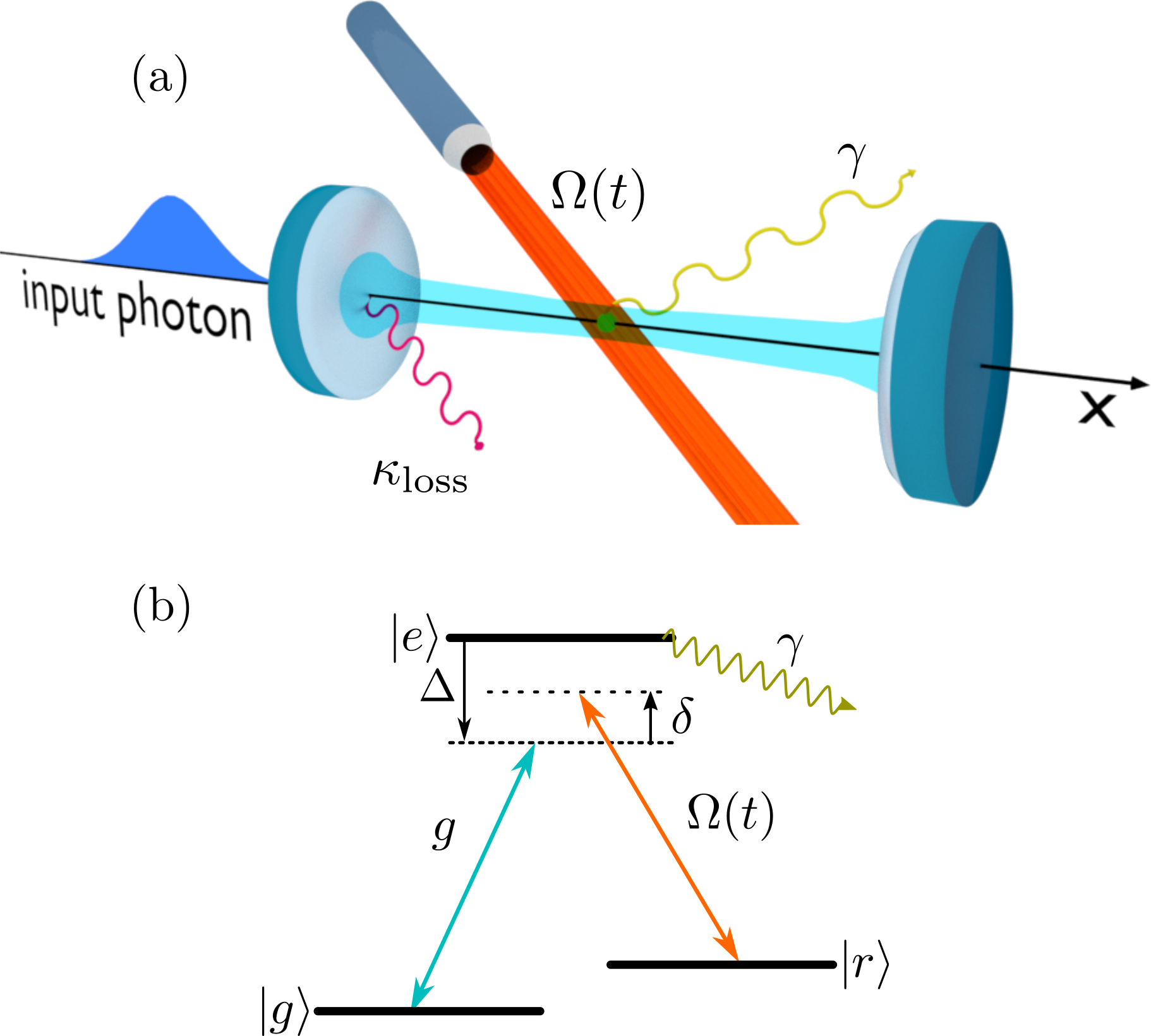
Figure 1: Storage of a single photon in the electronic state of a single atom confined inside an optical resonator. (a) The photon wave packet propagates along a transmission line and impinges onto a cavity mirror. (b) The single photon is absorbed by the cavity, which drives the atomic transition $|g\rangle\to|e\rangle$. An additional laser couples to the atomic transition $|r\rangle\to|e\rangle$. The dynamics of storage is tailored by optimizing the functional dependence of the laser amplitude on time, $\Omega(t)$: Ideally, the atom undergoes a Raman transition to the final state $|r\rangle$ and the photon is stored. We analyse the storage efficiency including the spontaneous decay with rate $\gamma$ of the excited state and photon absorption or scattering at the cavity mirrors via an incoherent process at rate ${\kappa_{\mathrm{loss}}}$. Further parameters are defined in the text.

The purpose of this work is to provide a systematic theoretical analysis of the efficiency of protocols for a quantum memory for single photons, where information is stored in the electronic excitation of a single atom inside a high-finesse resonator. The qubit can be the photon polarization Reiserer2015 ; Fleischhauer2000 , or a time-bin superposition of photonic states Dilley2012 , and shall then be transferred into a superposition of atomic spin states.

The scheme is illustrated in Fig. 1: a photon propagating along a transmission line impinges on the cavity mirror, the storage protocol coherently transfers the photon into a metastable atomic state, here denoted by $|r\rangle$, with the help of an external laser. The protocols we analyse are based on the seminal proposal by Cirac et al. Cirac1997 . Here, we first compare adiabatic protocols, originally developed for atomic ensembles in bad cavities Fleischhauer2000 ; Gorshkov2007a as well as a protocol developed for any coupling regime for a single atom Dilley2012 . We then extend the protocol of Ref. Gorshkov2007a to quantum memories composed of single atoms confined inside a high-finesse resonator. We investigate how the storage efficiency is affected by parasitic losses at the cavity mirrors and whether these effects can be compensated by the dynamics induced by the laser pulse driving the atom. We finally extend our study to the non-adiabatic regime, and analyse the efficiency of storage of broadband photon pulses using optimal control.

This manuscript is organized as follows. In Sec. II we introduce the basic model, which we use in order to determine the efficiency of the storage process. In Sec. III we analyse the efficiency of protocols based on adiabatic dynamics in presence of irreversible cavity losses. In Sec. IV we investigate the storage efficiency when the photon coherence time does not fulfil the condition for adiabatic quantum dynamics. Here, we use optimal control theory to determine the shortest photon pulse that can be stored. The conclusions are drawn in Sec. V. The appendices provide further details of the analyses presented in Sec. III.

II Basic model

The basic elements of the dynamics are illustrated in Fig. 1. A photon propagates along the transmission line and impinges on the mirror of a high-finesse cavity. Here, it interacts with a cavity mode at frequency $\omega_{\mathrm{c}}$. The cavity mode, in turn, couples to a dipolar transition of a single atom, which is confined within the resonator. We denote by $|g\rangle$ the initial electronic state in which the atom is prepared, it is a metastable state and it performs a transition to the excited state $|e\rangle$ by absorbing a cavity photon. The relevant atomic levels are shown in subplot (b): they are two meta-stable states, $|g\rangle$ and $|r\rangle$, which are coupled by electric dipole transitions to a common excited state $|e\rangle$ forming a $\Lambda$ level scheme. Transition $|r\rangle\to|e\rangle$ is driven by a laser, which we model by a classical field.

In order to describe the dynamics of the photon impinging onto the cavity mirror we resort to a coherent description of the modes of the electromagnetic field outside the resonator. The incident photon is an excitation of the external modes, and it couples with the single mode of a high-finesse resonator via the finite transmittivity of the mirror on which the photon is incident.

In this section we provide the details of our theoretical model and introduce the physical quantities which are relevant to the discussions in the rest of this paper.

II.1 Master equation

The state of the system, composed of the cavity mode, the atom, and the modes of the transmission line, is described by the density operator $\hat{\rho}$. Its dynamics is governed by the master equation ($\hbar=1$)

$$\partial_{t}\hat{\rho}=-\mathrm{i}[\hat{H}(t),\hat{\rho}]+\mathcal{L}_{\mathrm{dis}}\hat{\rho}\,,$$ (1)

where Hamiltonian $\hat{H}(t)$ describes the coherent dynamics of the modes of the electromagnetic field outside the resonator, of the single-mode cavity, of the atom’s internal degrees of freedom, and of their mutual coupling. The incoherent dynamics, in turn, is given by superoperator $\mathcal{L}_{\mathrm{dis}}$, and includes spontaneous decay of the atomic excited state, at rate $\gamma$, and cavity losses due to the finite transmittivity of the second cavity mirror as well as due to scattering and/or finite absorption of radiation at the mirror surfaces, at rate ${\kappa_{\mathrm{loss}}}$.

We first provide the details of the Hamiltonian. This is composed of two terms, $\hat{H}(t)=\hat{H}_{\mathrm{fields}}+\hat{H}_{\mathrm{I}}(t)$. The first term, $\hat{H}_{\mathrm{fields}}$, describes the coherent dynamics of the fields in absence of the atom. It reads

$$\hat{H}_{\mathrm{fields}}=\sum_{k}(\omega_{k}-\omega_{\mathrm{c}})\hat{b}_{k}^{\dagger}\hat{b}_{k}+\sum_{k}\lambda_{k}(\hat{a}^{\dagger}\hat{b}_{k}+\hat{b}_{k}^{\dagger}\hat{a}),$$ (2)

and is reported in the reference frame of the cavity mode frequency $\omega_{\mathrm{c}}$. Here, operators $\hat{b}_{k}$ and $\hat{b}_{k}^{\dagger}$ annihilate and create, respectively, a photon at frequency $\omega_{k}$ in the transmission line, with $[\hat{b}_{k},\hat{b}_{k^{\prime}}^{\dagger}]=\delta_{k,k^{\prime}}$. The modes $\hat{b}_{k}$ are formally obtained by quantizing the electromagnetic field in the transmission line and have the same polarization as the cavity mode. They couple with strength $\lambda_{k}$ to the cavity mode, which is described by a harmonic oscillator with annihilation and creation operators $a$ and $a^{\dagger}$, where $[\hat{a},\hat{a}^{\dagger}]=1$ and $[\hat{a},\hat{b}_{k}]=[\hat{a},\hat{b}_{k}^{\dagger}]=0$. In the rotating-wave approximation the interaction is of beam-splitter type and conserves the total number of excitations. The coupling $\lambda_{k}$ is related to the radiative damping rate of the cavity mode by the rate $\kappa=L|\lambda(\omega_{\mathrm{c}})|^{2}/c$, with $\lambda(\omega_{\mathrm{c}})$ the coupling strength at the cavity-mode resonance frequency Carmichael and $L$ the length of the transmission line. Note that $\kappa$ is the cavity decay rate because of transmission into the transmission line and is necessary for the storage, while ${\kappa_{\mathrm{loss}}}$ is the decay rate into other modes and is only detrimental.

The atom-photon interaction is treated in the dipole and rotating-wave approximation. The transition $|g\rangle\to|e\rangle$ couples with the cavity mode with strength (vacuum Rabi frequency) $g$. Transition $|r\rangle\to|e\rangle$ is driven by a classical laser with time-dependent Rabi frequency $\Omega(t)$, which is the function to be optimized in order to maximize the probability of transferring the excitation into state $|r\rangle$. The corresponding Hamiltonian reads

$$\hat{H}_{\mathrm{I}}=\delta\left|r\middle>\!\middle<r\right|-\Delta\left|e\middle>\!\middle<e\right|+\left[g\left|e\middle>\!\middle<g\right|\hat{a}+\Omega(t)\left|e\middle>\!\middle<r\right|+\mathrm{H.c.}\right],$$ (3)

where $\Delta=\omega_{\mathrm{c}}-\omega_{e}$ is the detuning between the cavity frequency $\omega_{\mathrm{c}}$ and the frequency $\omega_{e}$ of the $|g\rangle-|e\rangle$ transition, while $\delta=\omega_{r}+\omega_{\mathrm{L}}-\omega_{\mathrm{c}}$ is the two-photon detuning which is evaluated using the central frequency $\omega_{\mathrm{L}}$ of the driving field $\Omega(t)$. Here, we denote by $\omega_{r}=(E_{r}-E_{g})/\hbar$ the frequency difference (Bohr frequency) between the state $|r\rangle$ (of energy $E_{r}$) and the state $|g\rangle$ (of energy $E_{g}$). Unless otherwise stated, in the following we assume that the condition of two-photon resonance $\delta=0$ is fulfilled.

The irreversible processes that we consider in our theoretical description are (i) the radiative decay at rate $\gamma$ from the excited state $|e\rangle$, where photons are emitted into free field modes other than the modes $\hat{b}_{k}$ introduced in Eq. (2), and (ii) the cavity losses at rate ${\kappa_{\mathrm{loss}}}$ due to absorption and scattering at the cavity mirrors and to the finite transmittivity of the second mirror. We model each of these phenomena by Born-Markov processes described by the superoperators $\mathcal{L}_{\gamma}$ and $\mathcal{L}_{{\kappa_{\mathrm{loss}}}}$, respectively, such that $\mathcal{L}_{\mathrm{dis}}=\mathcal{L}_{\gamma}+\mathcal{L}_{{\kappa_{\mathrm{loss}}}}$ and

$$\mathcal{L}_{\gamma}\hat{\rho}=\gamma(2\left|\xi_{e}\middle>\!\middle<e\right|\hat{\rho}\left|e\middle>\!\middle<\xi_{e}\right|-\left|e\middle>\!\middle<e\right|\hat{\rho}-\hat{\rho}\left|e\middle>\!\middle<e\right|)\,,$$ (4a)

$$\mathcal{L}_{\kappa_{\mathrm{loss}}}\hat{\rho}={\kappa_{\mathrm{loss}}}(2\hat{a}\hat{\rho}\hat{a}^{\dagger}-\hat{a}^{\dagger}\hat{a}\hat{\rho}-\hat{\rho}\hat{a}^{\dagger}\hat{a})\,.$$ (4b)

Here, $|\xi_{e}\rangle$ is an auxiliary atomic state where the losses of atomic population from the excited state $|e\rangle$ are collected.

II.2 Initial state and target state

The model is one dimensional, the transmission line is at $x<0$, and the cavity mirror is at position $x=0$. The single incident photon is described by a superposition of single excitations of the modes of the external field Blum2013

$$|\psi_{\mathrm{sp}}\rangle=\sum_{k}\mathcal{E}_{k}\hat{b}_{k}^{\dagger}|\mathrm{vac}\rangle,$$ (5)

where $|\mathrm{vac}\rangle$ is the vacuum state and the amplitudes $\mathcal{E}_{k}$ fulfil the normalization condition $\sum_{k}|\mathcal{E}_{k}|^{2}=1$. For the studies performed in this work, we will consider the amplitudes

$$\mathcal{E}_{k}=\sqrt{\frac{c}{2L}}\int_{-\infty}^{\infty}{\rm d}t{\rm e}^{\mathrm{i}(kc-\omega_{\mathrm{c}})t}\mathcal{E}_{\mathrm{in}}(t)$$ (6)

with $c$ the speed of light, $L$ the length of the transmission line, and

$$\mathcal{E}_{\mathrm{in}}(t)=\frac{1}{\sqrt{T}}\operatorname{sech}{\left(\frac{2t}{T}\right)}$$ (7)

the input amplitude at the position $x=0$, with $T$ the characteristic time determining the coherence time $T_{\mathrm{c}}$ of the photon, $T_{c}=\pi T/4\sqrt{3}$ (see definition in Eq. (10)). Our formalism applies to a generic input envelope, nevertheless the specific choice of Eq. (7) allows us to compare our results with previous studies, see Refs. Fleischhauer2000 ; Gorshkov2007a ; Dilley2012 . The total state of the system at the initial time $t=t_{1}$ is given by the input photon in the transmission line, the empty resonator, and the atom in state $|g\rangle$. In particular, the dynamics is analysed in the interval $t\in[t_{1},t_{2}]$, with $t_{1}<0$, $t_{2}>0$ and $|t_{1}|,t_{2}\gg T_{\mathrm{c}}$, such that (i) at the initial time there is no spatial overlap between the single photon and the cavity mirror and (ii) assuming that the cavity mirror is perfectly reflecting, at $t=t_{2}$ the photon has been reflected away from the mirror.

The initial state is described by the density operator $\rho(t_{0})=|\psi_{0}\rangle\langle\psi_{0}|$, where

$$|\psi_{0}\rangle=|g\rangle\otimes|0\rangle_{c}\otimes|\psi_{\mathrm{sp}}\rangle\,,$$ (8)

and $|0\rangle_{c}$ is the Fock state of the resonator with zero photons.

Our target is to store the single photon into the atomic state $|r\rangle$ by shaping the laser field $\Omega(t)$. When comparing different storage approaches, it is essential to have a figure of merit characterizing the performance of the process. In accordance with Ref. Gorshkov2007a we define the efficiency $\eta$ of the process as the ratio between the probability to find the excitation in the state $|\psi_{T}\rangle=|r\rangle\otimes|0\rangle_{c}\otimes|\mathrm{vac}\rangle$ at time $t$ and the number of impinging photons between $t_{1}$ and $t$, namely

$$\eta(t)=\frac{\langle\psi_{T}|\rho(t)|\psi_{T}\rangle}{\int_{t_{1}}^{t}|\mathcal{E}_{\mathrm{in}}(t)|^{2}\mathrm{d}t}\,,$$ (9)

where $t>t_{1}$ and the denominator is unity for $t\to t_{2}$. We note that states $|\psi_{0}\rangle$ and $|\psi_{T}\rangle$ are connected by the coherent dynamics via the intermediate states $|e\rangle\otimes|0\rangle_{c}\otimes|\mathrm{vac}\rangle$ and $|g\rangle\otimes|1\rangle_{c}\otimes|\mathrm{vac}\rangle$. These states are unstable, since they can decay via spontaneous emission or via the parasitic cavity losses. Moreover, the incident photon can be reflected off the cavity. The latter is a unitary process, which results in a finite probability of finding a photon excitation in the transmission line after the photon has reached the mirror. The choice of $\Omega(t)$ shall maximize the transfer $|\psi_{0}\rangle\to|\psi_{T}\rangle$ by minimizing the losses as well as reflection at the cavity mirror.

II.3 Relevant quantities

The transmission line is here modelled by a cavity of length $L$, with a perfect mirror at $x=-L$. The second mirror at $x=0$ coincides with the mirror of finite transmittivity, separating the transmission line from the optical cavity. The length $L$ is chosen to be sufficiently large to simulate a continuum of modes for all practical purposes. This requires that the distance between neighbouring frequencies is smaller than all characteristic frequencies of the problem. The smallest characteristic frequency is the bandwidth of the incident photon, which is the inverse of the photon duration in time. Since the initial state is assumed to be a single photon in a pure state, the latter coincides with the photon coherence time $T_{c}$ Muller2017 which is defined as

$$T_{\mathrm{c}}=\sqrt{\langle t^{2}\rangle-\langle t\rangle^{2}}$$ (10)

with $\langle t^{x}\rangle\equiv\int_{t_{1}}^{t_{2}}t^{x}|\mathcal{E}_{\mathrm{in}}(t)|^{2}\mathrm{d}t$, and

$$\int_{t_{1}}^{t_{2}}|\mathcal{E}_{\mathrm{in}}(t)|^{2}\mathrm{d}t=1-\varepsilon\,,$$ (11)

where $\varepsilon<10^{-5}$ for the choice $|t_{1}|=t_{2}=6T_{\mathrm{c}}$ and $L=12cT_{\mathrm{c}}$. The modes of the transmission line are standing waves with wave vector along the $x$ axis. For numerical purposes we take a finite number $N$ of modes around the cavity wave number $k_{\mathrm{c}}=\frac{\omega_{\mathrm{c}}}{c}$. Their wave numbers are

$$k_{n}=k_{\mathrm{c}}+\frac{n\pi}{L}\,,$$ (12)

while $n=-(N-1)/2,\dots,(N-1)/2$, and the corresponding frequencies are $\omega_{n}=ck_{n}$. We choose $N$ and $L$ so that our simulations are not significantly affected by the finite size of the transmission line and by the cutoff in the mode number $N$. We further choose $N$ in order to appropriately describe spontaneous decay by the cavity mode. This is tested by initialising the system with no atom and one cavity photon and choosing the parameters so to reproduce the exponential damping of the cavity field.

Note that a single mode of the cavity is sufficient to describe the interaction with a single photon if the photon frequencies lie in a range which is smaller than the free spectral range of the cavity and is centered around the frequency of the cavity mode. In this work we choose the central frequency of the photon to coincide with the cavity mode frequency $\omega_{\mathrm{p}}=\omega_{\mathrm{c}}$ and the spectrally broadest photon we consider (Figs. 5 and 6) spans about $16\times 2\pi\,\mathrm{MHz}$ around the cavity frequency $\omega_{\mathrm{c}}$. A cavity of $1\,\mathrm{cm}$ has a free spectral range of about $15\times 2\pi\,\mathrm{GHz}$ which is three orders of magnitudes larger than the bandwidth of the photon. This justifies the approximation to a single mode cavity. The employed formalism can be applied to photons with other center frequencies as well, if the number of modes $N$ is chosen sufficiently large and their center is appropriately shifted (c.f. eq. (12)).

Since the free field modes are included in the unitary evolution, it is possible to constantly monitor their state. The photon distribution in space at time $t$ is given by

$$P(x,t)=\frac{2}{L}\sum_{n,m=1}^{N}\rho_{nm}(t)\sin\left(n\frac{\pi}{L}x\right)\sin\left(m\frac{\pi}{L}x\right),$$ (13)

where $\rho_{nm}(t)={\rm Tr}\{{\hat{\rho}(t)}\left|1_{m}\middle>\!\middle<1_{n}\right|\}$ and $|1_{n}\rangle=b_{k_{n}}^{\dagger}|\rm vac\rangle$.

A further important quantity characterizing the coupling between cavity mode and atom is the cooperativity $C$, which reads Gorshkov2007a

$$C=\frac{g^{2}}{\kappa\gamma}\,.$$ (14)

The cooperativity sets the maximum storage efficiency in the limit in which the cavity can be adiabatically eliminated from the dynamics of the system Gorshkov2007a , which corresponds to assuming the condition

$$\gamma CT_{\mathrm{c}}\gg 1\,.$$ (15)

In this limit, in fact, the state $|g\rangle\otimes|1\rangle_{c}\otimes|\text{vac}\rangle$ can be eliminated from the dynamics. Then, the efficiency satisfies $\eta(t)\leq\eta_{\mathrm{max}}$ where the maximal efficiency $\eta_{\mathrm{max}}$ reads Gorshkov2007a

$$\eta_{\mathrm{max}}=\frac{C}{1+C}.$$ (16)

The maximal efficiency $\eta_{\mathrm{max}}$ is reached for any input photon envelope $\mathcal{E}_{\mathrm{in}}(t)$ and detuning $\Delta$, provided the adiabatic condition (15) is fulfilled.

In our study we also determine the probability that the photon is in the transmission line,

$$P_{r}(t)=\sum_{k}{\rm Tr}\{\hat{\rho}(t)|1_{k}\rangle\langle 1_{k}|\},$$ (17)

the probability that spontaneous emission occurs,

$$P_{s}(t)={\rm Tr}\{\hat{\rho}(t)|\xi_{e}\rangle\langle\xi_{e}|\},$$ (18)

and finally, the probability that cavity parasitic losses take place,

$$P_{\mathrm{loss}}(t)=\operatorname{Tr}\left\{\hat{\rho}(t)\left|g,0_{c},\text{vac}\middle>\!\middle<g,0_{c},\text{vac}\right|\right\}.$$ (19)

By means of these quantities we gain insight into the processes leading to optimal storage.

III Storage in the adiabatic regime

In this section we determine the efficiency of storage protocols derived in Refs. Fleischhauer2000 ; Gorshkov2007a ; Dilley2012 for the setup of Ref. Koerber2017 in the adiabatic regime. We then analyse how the efficiency of these protocols is modified by the presence of parasitic losses at rate ${\kappa_{\mathrm{loss}}}$. In this case, we find also an analytic result which corrects the maximal value of Eq. (16).

We remark that in Refs. Fleischhauer2000 ; Gorshkov2007a ; Dilley2012 the optimal pulses $\Omega(t)$ were analytically determined using input-output theory Walls1994 . In Refs. Fleischhauer2000 ; Gorshkov2007a the authors consider an atomic ensemble inside the resonator in the adiabatic regime. This regime consists in assuming the bad cavity limit $\kappa\gg g$ and the limit $\gamma T_{\mathrm{c}}C\gg 1$. The first assumption allows one to adiabatically eliminate the cavity field variables from the equations of motion, the second assumption permits one to eliminate also the excited state $|e\rangle$. In Ref. Dilley2012 a single atom is considered and there is no such adiabatic approximation, but the coupling with the external field is treated using a phenomenological model.

Here we simulate the full Hamiltonian dynamics of the external field in the transmission line and consider a quantum memory composed of a single atom inside a reasonably good cavity. The parameters we refer to in our study are the ones of the setup of Ref. Koerber2017 :

$$(g,\kappa,\gamma)=(4.9,2.42,3.03)\times 2\pi\,\mathrm{MHz},$$ (20)

corresponding to the cooperativity $C=3.27$ and to the maximal storage efficiency $\eta_{\mathrm{max}}=0.77$. When we analyse the dependence of the efficiency on $\gamma$ or $\kappa$, we vary the parameters around the values given in Eq. (20).

III.1 Ideal resonator

We first review the requirements and results of the individual protocols of Refs. Fleischhauer2000 ; Gorshkov2007a ; Dilley2012 and investigate their efficiency for a single-atom quantum memory. The works of Refs. Fleischhauer2000 ; Gorshkov2007a ; Dilley2012 determine the form of the optimal pulse $\Omega(t)$ for cavities with cooperativities $C\geq 1$. The optimal pulse is found by imposing similar, but not equivalent requirements. In Refs. Fleischhauer2000 ; Dilley2012 the authors determine $\Omega(t)$ by imposing impedance matching, namely, that there is no photon reflected back by the cavity mirror. In Ref. Gorshkov2007a the pulse $\Omega(t)$ warrants maximal storage, namely, maximal probability of transferring the photon into the atomic excitation $|r\rangle$. The latter requirement corresponds to maximizing the storage efficiency $\eta$ defined in Eq. (9).

In detail, in Ref. Fleischhauer2000 the authors determine the optimal pulse $\Omega(t)$ that suppresses back-reflection from the cavity and warrants that the dynamics follows adiabatically the dark state of the system composed by cavity and atom. For this purpose the authors impose that the cavity field is resonant with the transition $|g\rangle\to|e\rangle$, namely $\Delta=0$. They further require that the coherence time $T_{\mathrm{c}}$ is larger than the cavity decay time, $\kappa T_{\mathrm{c}}\gtrsim 1$. Under these conditions the optimal pulse $\Omega(t)=\Omega^{\mathrm{F}}(t)$ reads

$$\Omega^{\mathrm{F}}(t)=\frac{g\mathcal{E}_{\mathrm{in}}(t)}{\sqrt{c_{1}+2\kappa\int_{t_{1}}^{t}|\mathcal{E}_{\mathrm{in}}(t^{\prime})|^{2}\mathrm{d}t^{\prime}-|\mathcal{E}_{\mathrm{in}}(t)|^{2}}}\,,$$ (21)

where $c_{1}$ regularize $\Omega^{\mathrm{F}}(t)$ for $t\to t_{1}$. The work in Ref. Dilley2012 imposes the suppression of the back-reflected photon without any adiabatic approximation and finds the optimal pulse $\Omega(t)=\Omega^{\mathrm{D}}(t)$, which takes the form

$$\Omega^{\mathrm{D}}(t)=\frac{g\mathcal{E}_{\mathrm{in}}(t)+\left(\dot{\mathcal{F}}(t)+\gamma\mathcal{F}(t)\right)/g}{\sqrt{2\kappa\rho_{0}+2\kappa\int\limits_{t_{1}}^{t}|\mathcal{E}_{\mathrm{in}}(t^{\prime})|^{2}-|\mathcal{E}_{\mathrm{in}}(t)|^{2}-\mathcal{D}(t)}},$$ (22)

with

$$\mathcal{D}(t)=2\gamma\int\limits_{t_{1}}^{t}|\mathcal{F}(t^{\prime})|^{2}\mathrm{d}t^{\prime}+|\mathcal{F}(t)|^{2}\,.$$ (23)

and $\mathcal{F}(t)=\dot{\mathcal{E}_{\mathrm{in}}}(t)-\kappa\mathcal{E}_{\mathrm{in}}(t)$. Coefficient $\rho_{0}$ accounts for a small initial population in the target state $|r\rangle$ and it is relevant in order to avoid divergences in Eq. (22) for $t\to t_{1}$, see Ref. Dilley2012 for an extensive discussion. The pulse $\Omega^{\mathrm{F}}(t)$ of Eq. (21) can be recovered from Eq. (22) by imposing the conditions

$$\dot{\mathcal{F}}(t)+\gamma\mathcal{F}(t)=0,\,$$ (24a)

$$-|\mathcal{F}(t_{1})|^{2}+2\kappa\rho_{0}=c_{1}.$$ (24b)

The control pulse $\Omega^{\mathrm{D}}(t)$ can be considered as a generalization of $\Omega^{\mathrm{F}}(t)$ since it is determined by solely imposing quantum impedance matching.

In Ref. Gorshkov2007a the authors determine the amplitude $\Omega(t)$ that maximizes the efficiency $\eta$. This condition is not equivalent to imposing impedance matching. In fact, while in the case of impedance matching major losses through the excited state $|e\rangle$ are acceptable in order to minimize the probability of photon reflection, in the case of maximum transfer efficiency $\eta$ those losses are detrimental and thus have to be minimized. The optimal pulse $\Omega(t)=\Omega^{\mathrm{G}}(t)$ is determined for a generic detuning $\Delta$ by using an analytical model based on the adiabatic elimination of the excited state $|e\rangle$ of the atom and of the cavity field in the bad cavity limit $\kappa\gg g$. It reads

$$\Omega^{\mathrm{G}}(t) {}=\frac{\gamma(1+C)+\mathrm{i}\Delta}{\sqrt{2\gamma(1+C)}}\frac{\mathcal{E}_{\mathrm{in}}(t)}{\sqrt{\int_{t_{1}}^{t}|\mathcal{E}_{\mathrm{in}}(t^{\prime})|^{2}\mathrm{d}t^{\prime}}}$$ (25)

$$\times\exp\left({-\mathrm{i}\frac{\Delta}{2\gamma(1+C)}\ln{\int_{t_{1}}^{t}|\mathcal{E}_{\mathrm{in}}(t^{\prime})|^{2}\mathrm{d}t^{\prime}}}\right)\,.$$

In the limit in which the adiabatic conditions are fulfilled, this control pulse allows for storage with efficiency $\eta_{\mathrm{max}}$, Eq. (16). This efficiency approaches unity for cooperativities $C\gg 1$.

We start by integrating numerically the master equation for a single atom (1) after setting ${\kappa_{\mathrm{loss}}}=0$, namely, by neglecting parasitic losses. We determine the storage efficiency at the time $t_{2}$, which we identify by taking $t_{2}\gg T_{\mathrm{c}}$ for different choices of the control field $\Omega=\Omega^{\mathrm{G}},\Omega^{\mathrm{F}},\Omega^{\mathrm{D}}$ in Hamiltonian (3). Numerically, $t_{2}$ corresponds to the time the photon would need to be reflected back into the initial position, assuming that the partially reflecting mirror is replaced by a perfect mirror. Our numerical simulations are performed for a single atom in a resonator in the good cavity limit.

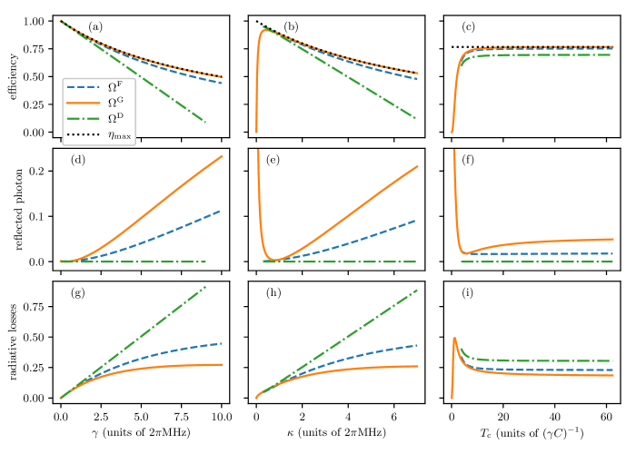
Figure 2: Comparison between the protocols of Refs. Fleischhauer2000 ; Gorshkov2007a ; Dilley2012 . (Upper row) Storage efficiency $\eta$, Eq. (9), (central row) probability that the photon is reflected $P_{r}$, Eq. (17), and (bottom row) probability of spontaneous emission, Eq. (18), evaluated at time $t_{2}=6T_{\mathrm{c}}$ by integrating numerically Eq. (1) for ${\kappa_{\mathrm{loss}}}=0$. The quantities are reported as a function of (left column) the decay rate $\gamma$ from the excited state (for $\kappa=\kappa_{0}$ and $T_{\mathrm{c}}=T_{\mathrm{c}}^{0}$), (central column) the decay rate $\kappa$ of the cavity field (for $\gamma=\gamma_{0}$ and $T_{\mathrm{c}}=T_{\mathrm{c}}^{0}$) and (right column) the coherence time of the photon $T_{\mathrm{c}}$ (in units of $1/(\gamma C)$ and for $\kappa=\kappa_{0}$ and $\gamma=\gamma_{0}$). The three different lines $\Omega^{\mathrm{F}}$, $\Omega^{\mathrm{D}}$, and $\Omega^{\mathrm{G}}$ refer to the evolution with the respective control pulse (see Eqs. (21), (22), (25), respectively). The dotted lines in panels (a)(b)(c) correspond to the maximum efficiency $\eta=C/(1+C)$, Eq. (16). Here, $(g,\kappa_{0},\gamma_{0})=(4.9,2.42,3.03)\times 2\pi\,\mathrm{MHz}$ and $T_{\mathrm{c}}^{0}=0.5\,\mathrm{\mu s}$. The input pulse $\mathcal{E}_{\mathrm{in}}(t)$ is given in Eq. (7), at the initial time $t_{1}=-6T_{\mathrm{c}}$ the pulse has negligible overlap with the cavity mode. The transmission line has length $L=\max(12cT_{\mathrm{c}},15c/\kappa)$ and $211$ equispaced modes. With this choice the frequency range of the modes included in the simulation is about $40\kappa$ around the cavity frequency $\omega_{\mathrm{c}}$.

Figures 2 display the efficiency and the losses as a function of $\kappa$, $\gamma$, and of the coherence time $T_{c}$ of the photon (and thus of the adiabatic parameter $\gamma T_{\mathrm{c}}C$). Each curve corresponds to the different control pulses in the Hamiltonian (3) according to the three protocols. In subplot (a) we observe that the efficiency reached with the pulse $\Omega^{\mathrm{G}}(t)$ corresponds to the maximum theoretical efficiency $\eta_{\mathrm{max}}$, while the efficiency with $\Omega^{\mathrm{D}}$ is the smallest. In subplot (b) it is visible that the control pulse $\Omega^{\mathrm{G}}(t)$ warrants the maximum efficiency even down to values of $\kappa$ of the order of $\kappa\sim g/5$. Subplot (c) displays the efficiency as a function of the adiabatic parameter $\gamma T_{\mathrm{c}}C$: the protocol $\Omega^{\mathrm{G}}(t)$ reaches the maximum theoretical efficiency $\eta_{\mathrm{max}}$ for $\gamma T_{\mathrm{c}}C\gtrsim 20$, while the other protocols have smaller efficiency for all values of $T_{\mathrm{c}}$. Figures 2(d)(e)(f) report the probability that the photon is reflected back into the transmission line, eq. (17). It is evident that protocol $\Omega^{\mathrm{D}}$ perfectly suppresses the back reflection probability in every regime here considered. However in the non-adiabatic regime (subplots (c)(f)(i), $\gamma T_{\mathrm{c}}C\lesssim 20$) the protocol $\Omega^{\mathrm{D}}$, as well as the protocol $\Omega^{\mathrm{F}}$, requires an increasing maximum Rabi frequency for decreasing $T_{\mathrm{c}}$. At the value of about $\gamma T_{\mathrm{c}}C\approx 3.74$ the Rabi frequency is so high that it is not anymore manageable by our numerical solver, for this reason the plots for the protocols $\Omega^{\mathrm{D}}$ and $\Omega^{\mathrm{F}}$ are reported for $\gamma T_{\mathrm{c}}C\gtrsim 3.74$. The same happens for small values of $\kappa$, subplots (b)(e)(h): in this case the plots for the protocols $\Omega^{\mathrm{D}}$ and $\Omega^{\mathrm{F}}$ are reported for $\kappa\gtrsim 0.3\times 2\pi\,\mathrm{MHz}$. The diverging Rabi frequency can be avoided by an appropriate choice of the parameters $c_{1}$ and $\rho_{0}$ in Eqs. (21) and (22), respectively. Figures 2(g)(h)(i) report the losses via spontaneous emission of the atom, Eq. (18): while these losses are acceptable in order to minimize the back-reflected photon, they are detrimental for the intent of populating the target state $|r\rangle$. Protocol $\Omega^{\mathrm{D}}$, which perfectly suppresses the back reflected photon, has the highest losses via spontaneous emission, which in the end leads to a lower efficiency $\eta$. Protocol $\Omega^{\mathrm{G}}$ in turn, has the lowest radiative losses and it allows for the transfer with the maximal efficiency $\eta_{\mathrm{max}}$. Protocol $\Omega^{\mathrm{F}}$ tries to minimize reflection of the photon at the cavity mirror. However, since $\Omega^{\mathrm{F}}$ is derived with some approximations, it does not suppress completely the reflection and its final efficiency is between the ones of the other two protocols.

An important general result of this study is that the bad cavity limit is not essential for reaching the maximal efficiency as long as the dynamics is adiabatic: the relevant parameter is in fact the cooperativity.

III.2 Parasitic losses

The protocols so far discussed assume an ideal optical resonator. In this section we analyse how their efficiency is modified by the presence of parasitic losses, here described by the superoperator $\mathcal{L}_{{\kappa_{\mathrm{loss}}}}$ in Eq. (4b). In particular, we derive the maximal efficiency the protocols can reach as a function of ${\kappa_{\mathrm{loss}}}>0$.

We first numerically determine the efficiency of the individual protocols as a function of ${\kappa_{\mathrm{loss}}}$ for $T_{\mathrm{c}}=0.5\,\mathrm{\mu s}$. Figure 3(a) displays $\eta$ for $\Omega=\Omega^{\mathrm{G}},\Omega^{\mathrm{D}},\Omega^{\mathrm{F}}$. It is evident that the effect of losses is detrimental, for instance it leads to a definite reduction of the maximal efficiency from $\eta=0.77$ down to $\eta=0.68$ for ${\kappa_{\mathrm{loss}}}\sim 0.1\kappa$. This result can be improved by identifying a control field $\Omega={\Omega^{\mathrm{X}}}$ which compensates, at least partially, the effects of these parasitic losses. The control field ${\Omega^{\mathrm{X}}}(t)$ is derived in Sec. III.3 using the input-output formalism: it corresponds to performing the substitution $\kappa\to\kappa+{\kappa_{\mathrm{loss}}}$ in the functional form $\Omega^{\mathrm{G}}(t)$ of Eq. (25). Specifically, it reads

$${\Omega^{\mathrm{X}}}(t) = \frac{\gamma(1+C^{\prime})+\mathrm{i}\Delta}{\sqrt{2\gamma(1+C^{\prime})}}\frac{\mathcal{E}_{\mathrm{in}}(t)}{\sqrt{\int_{t_{1}}^{t}|\mathcal{E}_{\mathrm{in}}(t^{\prime})|^{2}\mathrm{d}t^{\prime}}}$$

$$\times\exp\left({-\mathrm{i}\frac{\Delta}{2\gamma(1+C^{\prime})}\ln{\int_{t_{1}}^{t}|\mathcal{E}_{\mathrm{in}}(t^{\prime})|^{2}\mathrm{d}t^{\prime}}}\right)\,,$$

with the modified cooperativity

$$C^{\prime}=\frac{g^{2}}{\gamma(\kappa+{\kappa_{\mathrm{loss}}})}\,.$$ (27)

When the control pulse ${\Omega^{\mathrm{X}}}(t)$ is used, the efficiency of the process corresponds to the maximal efficiency $\eta^{\prime}_{\mathrm{max}}$, which is now given by

$$\eta^{\prime}_{\mathrm{max}}=\frac{\kappa}{\kappa+{\kappa_{\mathrm{loss}}}}\frac{C^{\prime}}{1+C^{\prime}}\,.$$ (28)

Clearly, $\eta^{\prime}_{\mathrm{max}}\leq\eta_{\mathrm{max}}$, while the equality holds for ${\kappa_{\mathrm{loss}}}=0$.

Figure 3: Efficiency of storage protocols in the adiabatic regime as a function of the rate of parasitic losses ${\kappa_{\mathrm{loss}}}$ (in units of $\kappa$). (a) Storage efficiency, Eq. (9), (b) the probability that the photon is reflected, Eq. (17), (c) the probability of spontaneous decay, Eq. (18), and (d) the probability of parasitic losses, Eq. (19), evaluated at time $t_{2}=6T_{\mathrm{c}}$ and for $(g,\kappa,\gamma)=(4.9,2.42,3.03)\times 2\pi\,\mathrm{MHz}$, $T_{\mathrm{c}}=0.5\,\mathrm{\mu s}$. The other parameters are the same as in Fig. 2. The lines ${\Omega^{\mathrm{X}}}$, $\Omega^{\mathrm{F}}$, $\Omega^{\mathrm{D}}$, and $\Omega^{\mathrm{G}}$ refer to the evolution with the respective control pulse (resp. Eqs. (III.2), (21), (22), (25)). The dotted line in (a) corresponds to the value of $\eta^{\prime}_{\mathrm{max}}$, Eq. (28).

By inspecting the numerical results, we note that the efficiency obtained using ${\Omega^{\mathrm{X}}}$ is always higher than the one reached by the other protocols. Even though for some values of ${\kappa_{\mathrm{loss}}}$ the efficiencies using different control fields may approach the one found with ${\Omega^{\mathrm{X}}}$, yet the dynamics are substantially different. This is visible by inspecting the probability that the photon is reflected, the radiative losses, and the parasitic losses, as a function of ${\kappa_{\mathrm{loss}}}$ as shown in Figs. 3(b)(c)(d), respectively: Each pulse distributes the losses in a different way, with ${\Omega^{\mathrm{X}}}(t)$ interpolating among the different strategies in order to maximize the efficiency.

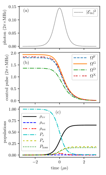
Figure 4: Dynamics of storage. (a) Photon envelope $|\mathcal{E}_{\mathrm{in}}(t)|^{2}$, Eq. (7), as a function of time. (b) Time dependence of the control pulses $\Omega^{\mathrm{F}}(t)$, $\Omega^{\mathrm{G}}(t)$, $\Omega^{\mathrm{D}}(t)$, and ${\Omega^{\mathrm{X}}}(t)$ (resp. Eqs. (21), (25), (22), (III.2)). (c) Time evolution of the diagonal elements of the density matrix when the atom is driven by ${\Omega^{\mathrm{X}}}$. The curves are the population $\rho_{rr}$ of state $|r\rangle$, the population $\rho_{ee}$ of state $|e\rangle$, the probability that there is one photon in the cavity $\rho_{aa}$, the probability that the photon is in the transmission line $P_{r}$, Eq. (17), the probability of spontaneous decay, Eq. (18) $P_{s}$, and the probability of cavity parasitic losses $P_{\mathrm{loss}}$, Eq. (19). The parameters are $(g,\kappa,\gamma,{\kappa_{\mathrm{loss}}})=(4.9,2.42,3.03,0.33)\times 2\pi\,\mathrm{MHz}$, $\Delta=0$ and $T_{\mathrm{c}}=0.5\,\mathrm{\mu s}$.

Figure 4 shows the evolution of the system for $T_{\mathrm{c}}=0.5\,\mathrm{\mu s}$. Fig. 4(a) displays the envelope in time $|\mathcal{E}_{\mathrm{in}}(t)|^{2}$ for the photon given in eq. (7), which is the one used also in this simulation. Fig. 4(b) displays the control pulse shapes of the protocols $\Omega^{\mathrm{F}}$, $\Omega^{\mathrm{G}}$, $\Omega^{\mathrm{D}}$, of Refs. Fleischhauer2000 ; Gorshkov2007a ; Dilley2012 and ${\Omega^{\mathrm{X}}}$ derived in this work (the pulse shapes are given analytically in Eqs. (21), (25), (22), (III.2)). Fig. 4(c) shows the population of the states and the losses during the evolution when the atom is driven by ${\Omega^{\mathrm{X}}}(t)$. The efficiency of the transfer, Eq. (9), corresponds to the population of the state $|r\rangle$, $\rho_{rr}$. For the parameters of Ref. Koerber2017 the final efficiency is $\eta(t_{2})\approx\eta^{\prime}_{\mathrm{max}}\approx 0.653$.

In the next subsection we report the derivation of ${\Omega^{\mathrm{X}}}$ and $\eta^{\prime}_{\mathrm{max}}$ by means of the input-output formalism.

III.3 Maximal efficiency in presence of parasitic losses

In this section we generalize the adiabatic protocol of Ref. Gorshkov2007a in order to identify the control field that maximizes the storage efficiency and to determine the maximum storage efficiency one can reach. The derivation presented in this section is based on the input-output formalism and it delivers Eq. (III.2) and Eq. (28).

We first justify the result for Eq. (28) using a time reversal argument applied in Refs. Gorshkov2007a ; Gorshkov2007b . Let us consider retrieval of the photon, assuming the atom is initially in state $|r\rangle$ and there is neither external nor cavity field. Then, in order to retrieve the photon, the control pulse $\Omega(t)$ shall drive the transition $|r\rangle\to|e\rangle$ such that at the end of the process the state $|r\rangle$ is completely empty. The excited state $|e\rangle$ dissipates the excitation with probability $1/(1+C^{\prime})$, while it can emit into the cavity mode with probability $C^{\prime}/(1+C^{\prime})$. When the cavity mode is populated, a fraction ${\kappa_{\mathrm{loss}}}/(\kappa+{\kappa_{\mathrm{loss}}})$ is lost, while the fraction $\kappa/(\kappa+{\kappa_{\mathrm{loss}}})$ is emitted via the coupling mirror into the transmission line. From this argument one finds that the probability of retrieval is given by Eq. (28). Using the time reversal argument, this is also the efficiency of storage.

We now derive this result as well as ${\Omega^{\mathrm{X}}}(t)$ starting from the retrieval process and then applying the time reversal argument. For this purpose, we restrict the dynamics to the Hilbert space ${\mathcal{H}}$ composed by the states $\{|g,1_{c},\text{vac}\rangle,|e,0_{c},\text{vac}\rangle,|r,0_{c},\text{vac}\rangle,|g,0_{c},1_{k}\rangle:1\leq k\leq N\}$. In ${\mathcal{H}}$ the probability is not conserved due to leakage via spontaneous decay and via parasitic cavity losses. Therefore, a generic state in ${\mathcal{H}}$ takes the form $|\phi(t)\rangle=c(t)|g,1_{c},\text{vac}\rangle+e(t)|e,0_{c},\text{vac}\rangle+r(t)|r,0_{c},\text{vac}\rangle+\sum_{k}\mathcal{E}_{k}(t)|g,0_{c},1_{k}\rangle$, it evolves according to a non-Hermitian Hamiltonian and its norm decays exponentially with time Moelmer1988 . We assume that at the initial time $t=t_{1}$ the probability amplitude $r(t_{1})$ equals $1$, while all other probability amplitudes vanish. The equations of motion for the probability amplitudes read

$$\dot{c}(t)=-\mathrm{i}ge(t)-\mathrm{i}\sqrt{2\kappa}\mathcal{E}_{\mathrm{in}}(t)-(\kappa+{\kappa_{\mathrm{loss}}})c(t),$$ (29a)

$$\dot{e}(t)=(\mathrm{i}\Delta-\gamma)e(t)-\mathrm{i}gc(t)-\mathrm{i}\Omega(t)r(t),$$ (29b)

$$\dot{r}(t)=-\mathrm{i}\Omega^{*}(t)e(t)\,,$$ (29c)

where we used the Markov approximation and the input-output formalism Walls1994 . We now assume the bad-cavity limit $\kappa\gg g$ and adiabatically eliminate the cavity field from the equations of motion (which corresponds to assuming $\dot{c}(t)\approx 0$ over the typical time scales of the other variables). In this limit the input-output operator relation, $\hat{\mathcal{E}}_{\mathrm{out}}(t)=\mathrm{i}\sqrt{2\kappa}\hat{a}(t)-\hat{\mathcal{E}}_{\mathrm{in}}(t)$, takes the form

$$\mathcal{E}_{\mathrm{out}}(t)=G\sqrt{2\gamma C}e(t)+\frac{\kappa-{\kappa_{\mathrm{loss}}}}{\kappa+{\kappa_{\mathrm{loss}}}}\mathcal{E}_{\mathrm{in}}(t)\,,$$ (30)

where

$$G=\kappa/(\kappa+{\kappa_{\mathrm{loss}}})$$

and $C$ is given in Eq. (14). This equation has to be integrated together with the equations

$$\dot{e}(t)=\left[\mathrm{i}\Delta-\gamma\left(1+GC\right)\right]e(t)-\mathrm{i}\Omega(t)r(t)-G\sqrt{2\gamma C}\mathcal{E}_{\mathrm{in}}(t)\,,$$ (31)

$$\dot{r}(t)=-\mathrm{i}\Omega^{*}(t)e(t)\,.$$ (32)

Our goal is to determine the retrieval efficiency assuming that at time $t=0$ there is no input photonic excitation, thus $\mathcal{E}_{\mathrm{in}}(t)=0$ at all times. Using these assumptions, the above equations can be cast into the form

$$\frac{\mathrm{d}}{\mathrm{d}t}\left(|e(t)|^{2}+|r(t)|^{2}\right)=-2\gamma\left(1+C^{\prime}\right)|e(t)|^{2}\,.$$ (33)

The probability that no excitations are left in the atom at time $t_{2}>0$ ($t_{2}\gg T_{\mathrm{c}}$) is the retrieval efficiency

$$\eta^{\prime}_{\mathrm{max}} =\int_{t_{1}}^{t_{2}}|\mathcal{E}_{\mathrm{out}}(t)|^{2}\mathrm{d}t=2G^{2}\gamma C\int_{t_{1}}^{t_{2}}|e(t)|^{2}\mathrm{d}t=$$ (34)

$$=\frac{-GC^{\prime}}{1+C^{\prime}}\left[|e(t)|^{2}+|r(t)|^{2}\right]_{t_{1}}^{t_{2}}=\frac{GC^{\prime}}{1+C^{\prime}}\,.$$

By means of the time reversal argument, this is also the storage efficiency.

The output field can be analytically determined by adiabatically eliminating the excited state from Eqs. (30). This leads to the expression

$$\mathcal{E}_{\mathrm{out}}(t)={} \mathrm{i}\sqrt{2\gamma GC^{\prime}}\frac{\Omega(t)}{\mathrm{i}\Delta-\gamma(1+C^{\prime})}$$ (35)

$$\times\exp\left(\int_{t_{1}}^{t}\frac{|\Omega(t^{\prime})|^{2}}{\mathrm{i}\Delta-\gamma(1+C^{\prime})}\mathrm{d}t^{\prime}\right)\,.$$

Integrating the norm squared of Eq. (35) one obtains

$$\begin{gathered}\left(G\frac{C^{\prime}}{1+C^{\prime}}\right)^{-1}\int_{t_{1}}^{t}|\mathcal{E}_{\mathrm{out}}(t^{\prime})|^{2}\mathrm{d}t^{\prime}=\\ =1-\exp\left[\frac{-2\gamma(1+C^{\prime})}{\gamma^{2}(1+C^{\prime})^{2}+\Delta^{2}}\int_{t_{1}}^{t}|\Omega(t^{\prime})|^{2}\mathrm{d}t^{\prime}\right]\,.\end{gathered}$$ (36)

We solve Eq. (36) to find $|\Omega(t)|$, while the phase of $\Omega(t)$ can be determined from Eq. (35). Finally, we obtain the control pulse ${\Omega^{\mathrm{X}}}_{\mathrm{retr}}(t)$ which retrieves the photon with efficiency $\eta^{\prime}_{\mathrm{max}}$. It reads

$${\Omega^{\mathrm{X}}}_{\mathrm{retr}}(t)=\frac{\gamma(1+C^{\prime})-\mathrm{i}\Delta}{\sqrt{2\gamma(1+C^{\prime})}}\frac{\mathcal{E}_{\mathrm{out}}(t)}{\sqrt{\int_{t}^{t_{2}}|\mathcal{E}_{\mathrm{out}}(t^{\prime})|^{2}\mathrm{d}t^{\prime}}}$$ (37)

$$\times\exp\left({\mathrm{i}\frac{\Delta}{2\gamma(1+C^{\prime})}\ln{\int_{t}^{t_{2}}(|\mathcal{E}_{\mathrm{out}}(t^{\prime})|^{2}/\eta^{\prime}_{\mathrm{max}})\mathrm{d}t^{\prime}}}\right)\,.$$

Using the time reversal argument, the control pulse ${\Omega^{\mathrm{X}}}(t)={\Omega^{\mathrm{X}}}^{*}_{\mathrm{retr}}(T-t)$ stores the time reversed input photon with $\mathcal{E}_{\mathrm{in}}(t)=\mathcal{E}_{\mathrm{out}}^{*}(T-t)/\sqrt{\eta^{\prime}_{\mathrm{max}}}$ and $T=t_{2}-t_{1}$, and it takes the form given in Eq. (III.2). This pulse has the same form as the pulse of Eq. (25), where now $C$ has been replaced by $C^{\prime}$ (or equivalently $\kappa\to\kappa+{\kappa_{\mathrm{loss}}}$).

III.4 Photon Retrieval

The generation of single photons with arbitrary shape of the wavepacket envelope in atom-cavity systems has been discussed theoretically in Gorshkov2007a ; Vasilev2010 and demonstrated experimentally in Keller2004 ; Nisbet-Jones2011 .

In Ref. Cirac1997 ; Gorshkov2007b it has been pointed out that photon storage and retrieval are connected by a time reversal transformation. This argument has profound implications. Consider for instance the pulse shape $\Omega(t)$ which optimally stores an input photon with envelope $\mathcal{E}_{\mathrm{in}}(t)$. This pulse shape is the time reversal of the pulse shape $\Omega_{\mathrm{retr}}(t)=\Omega^{*}(T-t)$ which retrieves a photon with envelope $\mathcal{E}_{\mathrm{out}}(t)=\mathcal{E}_{\mathrm{in}}^{*}(T-t)$ (here $T=t_{2}-t_{1}$). In this case, the storage efficiency is equal to the efficiency of retrieval and is limited by the cooperativity through the relation in Eq. (28). We have numerically checked that this is fulfilled by considering adiabatic retrieval and storage of a single photon through 5 nodes, consisting of 5 identical cavity-atom systems. We applied $\Omega_{\mathrm{retr}}(t)$ for the retrieval and the corresponding $\Omega(t)$ for the storage. Within the numerical error, we verified that the storage efficiency of each retrieved photon remains constant and equal to the one of the first retrieved photon.

IV Beyond adiabaticity

In this section we analyse the efficiency of storage of single photon pulses in the regime in which the adiabaticity condition Eq. (15) does not hold. Our treatment extends to single-atom quantum memories the approach that was applied to atomic ensemble in Refs. Novikova2007 ; Gorshkov2008 and allows us to identify the minimum coherence time scale of the photon pulse for which a given target efficiency can be reached.

Our procedure is developed as follows. We use the von-Neumann equation, obtained from Eq. (1) after setting $\gamma={\kappa_{\mathrm{loss}}}=0$, and resort to optimal control theory for identifying the control pulse $\Omega(t)=\Omega^{\mathrm{opt}}(t)$ that maximizes the storage efficiency for $\gamma={\kappa_{\mathrm{loss}}}=0$. Specifically, we make use of the GRAPE algorithm Khaneja2005 implemented in the library QuTiP Johansson2012-13 . We then determine the storage efficiency of the full dynamics, including spontaneous decay and cavity parasitic losses, by numerically integrating the master equation (1) using the pulse $\Omega^{\mathrm{opt}}(t)$. We show that the dynamics due to $\Omega^{\mathrm{opt}}(t)$ significantly differs from the adiabatic dynamics, and thereby improve the efficiency for short coherence times.

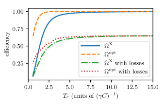
Figure 5: Storage efficiency $\eta$ at $t=t_{2}$ as a function of the coherence time of the single-photon pulse $T_{\mathrm{c}}$ (in units of $(\gamma C)^{-1}$). The legenda indicates the pulses used in the numerical integration of Eq. (1). The parameters are $(g,\kappa)=(4.9,2.42)\times 2\pi\,\mathrm{MHz}$, the lines labeled “with losses” refer to the efficiency of the process when $(\gamma,{\kappa_{\mathrm{loss}}})=(3.03,0.33)\times 2\pi\,\mathrm{MHz}$, otherwise $\gamma={\kappa_{\mathrm{loss}}}=0$; $t_{2}=-t_{1}=6T_{\mathrm{c}}$. The other parameters are given in Fig. 2.

Figure 5 displays the storage efficiency $\eta$ as a function of the photon coherence time $T_{\mathrm{c}}$ when the control pulse is ${\Omega^{\mathrm{X}}}(t)$, Eq. (III.2), and when instead the control pulse is found by means of the numerical procedure specified above, which we denote by $\Omega^{\mathrm{opt}}(t)$. The storage efficiency is reported for $\gamma={\kappa_{\mathrm{loss}}}=0$ and for $(\gamma,{\kappa_{\mathrm{loss}}})=(3.03,0.33)\times 2\pi\,\mathrm{MHz}$. The results show that optimal control, in the way we implement it, does not improve the maximal value of the storage efficiency, which seems to be limited by the value of $\eta_{\rm max}^{\prime}$, Eq. (28). We remark that this behaviour is generally encountered when applying optimal-control-based protocols to Markovian dynamics Koch2016 . Nevertheless, the protocols identified using optimal control extend the range of values of $T_{\mathrm{c}}$, where the maximal efficiency is reached, down to values where the adiabatic condition is not fulfilled. We further find that the optimized pulse we numerically identified in absence of losses provides an excellent guideline for optimizing the storage also in presence of losses.

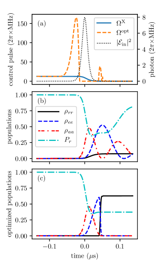
Figure 6: (a) Photon envelope $|\mathcal{E}_{\mathrm{in}}(t)|^{2}$, Eq. (7), and optimized pulse $\Omega^{\mathrm{opt}}(t)$ as a function of time (the initial guess pulse ${\Omega^{\mathrm{X}}}(t)$ is shown for comparison). Subplot (b) and (c) display the time evolution of the diagonal elements of the density matrix when the atom is driven by ${\Omega^{\mathrm{X}}}$ and $\Omega^{\mathrm{opt}}$, respectively. The curves are the population $\rho_{rr}$ of state $|r\rangle$, the population $\rho_{ee}$ of state $|e\rangle$, the probability that there is one photon in the cavity $\rho_{aa}$, and the probability that the photon is in the transmission line $P_{r}$, Eq. (17). The parameters are $(g,\kappa)=(4.9,2.42)\times 2\pi\,\mathrm{MHz}$, $\gamma={\kappa_{\mathrm{loss}}}=\Delta=0$ and $T_{\mathrm{c}}=0.009\,\mathrm{\mu s}$, thus the regime is non adiabatic as $T_{\mathrm{c}}\approx 0.57/(\gamma C)$. At $t=t_{2}$ the population $\rho_{rr}$ gives $\eta(t_{2})$. In this case the system has been simulated for a longer time interval: $t_{2}=-t_{1}=15T_{\mathrm{c}}$.

In order to get insight into the optimized dynamics we analyse the time dependence of the control pulse as well as the dynamics of cavity and atomic state populations for $T_{\mathrm{c}}=0.009\,\mathrm{\mu s}$, namely, when the dynamics is non-adiabatic. Figure 6(a) shows the time evolution of the pulse $\Omega^{\mathrm{opt}}(t)$ resulting from the optimization procedure in the non-adiabatic regime; the pulse ${\Omega^{\mathrm{X}}}(t)$ is shown for comparison. The efficiency of the transfer (when the losses are neglected) with the control pulse ${\Omega^{\mathrm{X}}}$ is $\eta^{\mathrm{X}}\approx 0.07<\eta_{\mathrm{max}}$ because the process is non adiabatic, while the efficiency reached with the optimized pulse $\Omega^{\mathrm{opt}}(t)$ is $\eta^{\mathrm{opt}}\approx 0.63$. The value of the solid green line at $t=t_{2}$ in Fig. 6(b) and  6(c) corresponds to the leftmost point in Fig. 5 for the case without losses. A double bump in the cavity population is visible in Fig. 6(b): this is due to the Jaynes-Cummings dynamics, and is thus the periodic exchange of population between the atomic excited state $|e\rangle$ and the cavity field. In Fig. 6(a) it is noticeable that the intensity of the optimized pulse exhibits a relatively high peak when the photon is impinging on the cavity. It corresponds to a way to perform impedance matching in order to maximize the transmission at the mirror, and it is related to the same dynamics which gives rise to the divergence of $\Omega^{\mathrm{F}}(t)$ and $\Omega^{\mathrm{D}}(t)$ which is found when they are applied in the non-adiabatic regime. After this the intensity of the control pulse vanishes and then exhibits a second maximum when the population of the excited state reaches the maximum: we verified that the area about this second “pulse” corresponds to the one of a $\pi$ pulse, thus transferring the population into state $|r\rangle$.

We now investigate the limit of optimal storage. For this purpose we determine the lower bound $T_{\mathrm{c}}^{\mathrm{min}}$ to the coherence time $T_{\mathrm{c}}$ of the photon, for which a given efficiency $\eta=\eta_{\mathrm{tr}}$ can be reached. For each value of $g$ and $T_{\mathrm{c}}$ we optimize the control pulse using GRAPE. For each $g$ we determine $\eta$ as a function of $T_{\mathrm{c}}$ and then extract $T_{\mathrm{c}}^{\mathrm{min}}=\min_{T_{\mathrm{c}}}\left\{T_{\mathrm{c}}:\eta(T_{\mathrm{c}})\geq\eta_{\mathrm{tr}}\right\}$. We then analyse how the minimum coherence time $T_{\mathrm{c}}^{\mathrm{min}}$ scales with the vacuum Rabi frequency $g$.

Figure 7 displays the minimum photon coherence time $T_{\mathrm{c}}^{\mathrm{min}}$ required for reaching the storage efficiency (a) $\eta_{\mathrm{tr}}=0.99$ and (b) $\eta_{\mathrm{tr}}=2/3$ as a function of the coupling constant $g$. We observe two behaviours, separated by the value $g=\kappa$: For $g\ll\kappa$, in the bad cavity limit, we extract the functional behaviour $T_{\mathrm{c}}^{\mathrm{min}}\propto 1/\gamma C=\kappa/g^{2}$. On the contrary, in the good cavity limit, $g>\kappa$, we find that $T_{\mathrm{c}}^{\mathrm{min}}\propto 1/\kappa$: The limit to photon storage is here determined by the cavity linewidth. The general behaviour as a function of $g$ interpolates between these two limits. This result shows that the photon can be stored as long as its spectral width is of the order of the linewidth of the dressed atomic state.

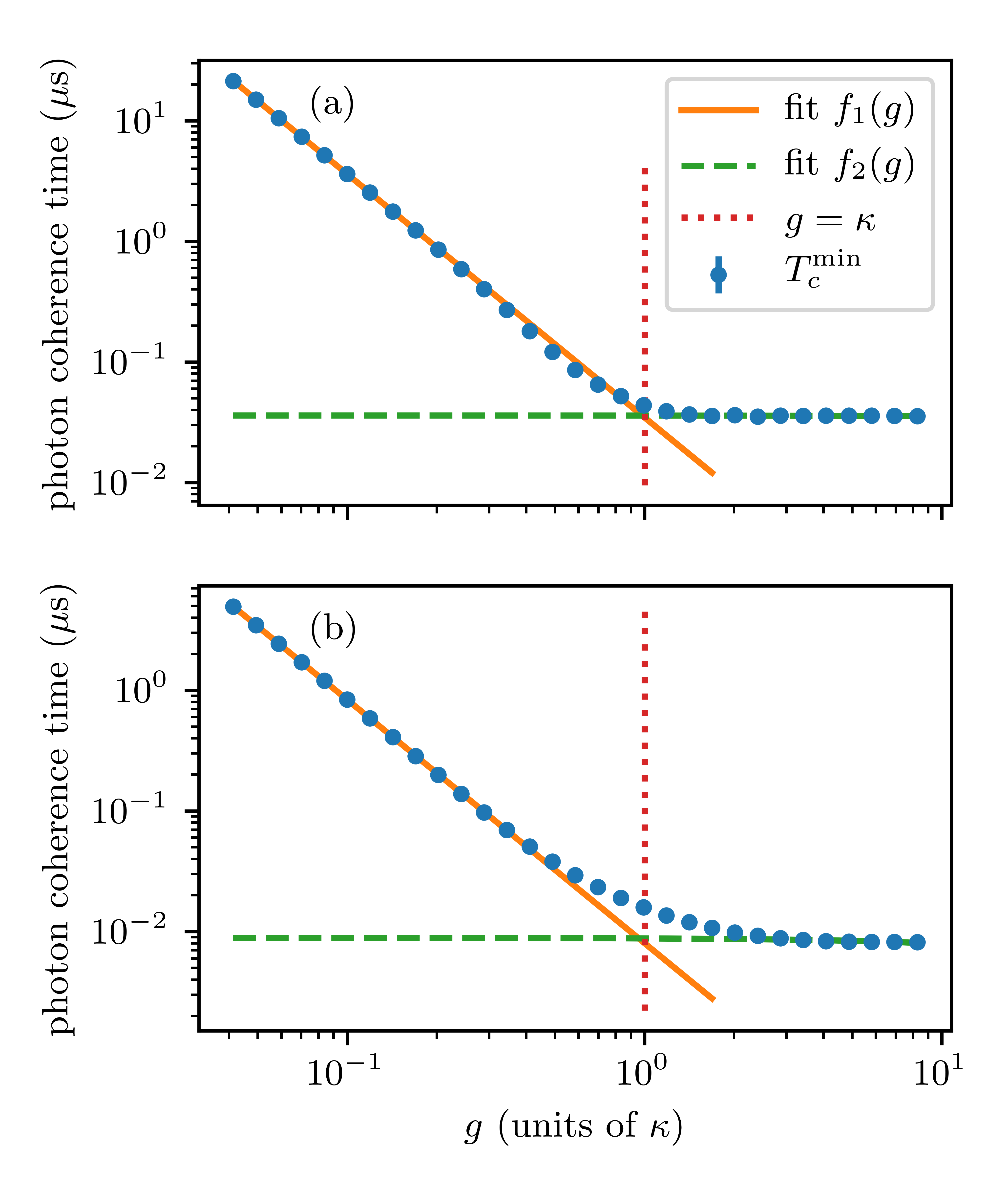
Figure 7: Minimum photon coherence time $T_{\mathrm{c}}^{\mathrm{min}}$ as a function of $g$ (in units of $\kappa$). The coherence time $T_{\mathrm{c}}^{\mathrm{min}}$ is the lower bound to the coherence time of photons which can be stored with efficiency (a) $\eta_{\mathrm{tr}}=0.99$ and (b) $\eta_{\mathrm{tr}}=2/3$ for $\gamma={\kappa_{\mathrm{loss}}}=\Delta=0$. The vertical dotted line shows the value $g=\kappa=2.42\times 2\pi\,\mathrm{MHz}$. The data in the region $g\ll\kappa$ and $g\gg\kappa$ have been fitted with the functions $f_{1}(g)=a\kappa/g^{2}$ and $f_{2}(g)=a^{\prime}/\kappa$, respectively.

V Conclusions

We have analysed the storage efficiency of a single photon by a single atom inside a resonator. We have focused on the good cavity limit and shown that, as in the bad cavity limit, the storage efficiency is bound by the cooperativity and the maximal value it can reach is given by Eq. (16). We have extended these predictions to the case in which the resonator undergoes parasitic losses. For this case we determined the maximal storage efficiency for an adiabatic protocol as well as the corresponding control field respectively given in Eq. (28) and Eq. (III.2). Numerical simulations show that protocols based on optimal control theory do not achieve higher storage efficiencies than $\eta_{\rm max}^{\prime}$. Nevertheless they can reach this upper bound even for spectrally-broad photon wave packets where the dynamics is non-adiabatic, as long as the spectral width is of the order of the linewidth of the dressed atomic state.

Our analysis shows that the storage efficiency is limited by parasitic losses. Nevertheless, we have demonstrated that these can be partially compensated by the choice of an appropriate control field. This result has been analytically derived for adiabatic protocols, yet it shows that extending optimal control theory to incoherent dynamics could provide new tools for efficient quantum memories.

Appendix A Input-output formalism

In input-output formalism Walls1994 the equation of motion are

$$\dot{\hat{a}}=-\mathrm{i}g\hat{\sigma}_{ge}-\mathrm{i}\sqrt{2\kappa}\hat{\mathcal{E}}_{\mathrm{in}}(t)-(\kappa+\kappa_{\mathrm{bad}})\hat{a}(t)+\hat{F}_{a},$$ (38)

$$\dot{\hat{\sigma}}_{gg}=\mathrm{i}g\hat{\sigma}_{eg}\hat{a}-\mathrm{i}g\hat{a}^{\dagger}\hat{\sigma}_{ge},$$

$$\dot{\hat{\sigma}}_{rr}=\mathrm{i}\Omega(t)\hat{\sigma}_{er}-\mathrm{i}\Omega^{*}(t)\hat{\sigma}_{re},$$

$$\begin{aligned} \dot{\hat{\sigma}}_{ee}={}&-\mathrm{i}g\hat{\sigma}_{eg}\hat{a}+\mathrm{i}g\hat{a}^{\dagger}\hat{\sigma}_{ge}-\mathrm{i}\Omega(t)\hat{\sigma}_{er}+{}\\ &{}+\mathrm{i}\Omega^{*}(t)\hat{\sigma}_{re}-\gamma\hat{\sigma}_{ee}+\hat{F}_{ee},\end{aligned}$$

$$\begin{aligned} \dot{\hat{\sigma}}_{ge}={}&\mathrm{i}\Delta\hat{\sigma}_{ge}+\mathrm{i}g(\hat{\sigma}_{ee}-\hat{\sigma}_{gg})\hat{a}-\mathrm{i}\Omega(t)\hat{\sigma}_{gr}+{}\\ &{}-\frac{\gamma}{2}\hat{\sigma}_{ge}+\hat{F}_{ge},\end{aligned}$$

$$\begin{aligned} \dot{\hat{\sigma}}_{er}={}&-\mathrm{i}\Delta\hat{\sigma}_{er}+\mathrm{i}g\hat{a}^{\dagger}\hat{\sigma}_{gr}+\mathrm{i}\Omega^{*}(t)(\hat{\sigma}_{rr}-\hat{\sigma}_{ee})+{}\\ &-\frac{\gamma}{2}\hat{\sigma}_{er}+\hat{F}_{er},\end{aligned}$$

$$\dot{\hat{\sigma}}_{gr}=\mathrm{i}g\hat{\sigma}_{er}\hat{a}-\mathrm{i}\Omega^{*}(t)\hat{\sigma}_{ge},$$

where $\hat{\sigma}_{jk}=\left|j\middle>\!\middle<k\right|$ are atomic operators and $\hat{F}_{a}$, $\hat{F}_{ee}$, $\hat{F}_{ge}$ and $\hat{F}_{er}$ are Langevin noise operators Cohen-Tannoudji1994 . The input operator for the quantum electromagnetic field is

$$\hat{\mathcal{E}}_{\mathrm{in}}(t)=\sqrt{\frac{Lc}{2\pi^{2}}}\int_{-\infty}^{\infty}e^{-\mathrm{i}kc(t-t_{1})}\hat{b}(k+k_{c},t=t_{1})\mathrm{d}k,$$ (39)

here $\hat{b}(k,t=t_{1})$ is the annihilation operator of the mode $k$ at the initial time $t=t_{1}$. The input output relation is given by

$$\hat{\mathcal{E}}_{\mathrm{out}}(t)=\mathrm{i}\sqrt{2\kappa}\hat{a}(t)-\hat{\mathcal{E}}_{\mathrm{in}}(t).$$ (40)

The equations of motion for $M\gg 1$ atoms in the cavity take the same form as Eqs. (38) when one performs the replacement $\hat{\sigma}_{jk}\to\sum_{i=1}^{N}\hat{\sigma}_{jk}^{i}$ Gorshkov2007a . In this case, one can make the approximations $\langle\tilde{\sigma}_{gg}(t)\rangle\approx M$, $\langle\tilde{\sigma}_{rr}(t)\rangle\approx\langle\tilde{\sigma}_{ee}(t)\rangle\approx\langle\tilde{\sigma}_{er}(t)\rangle=0$, where $\langle\cdot\rangle=\operatorname{Tr}\left(\rho_{0}\cdot\right)$ and $\rho_{0}$ is the initial state. Then, the set of equations (38) reduces to the equations of motion of a single photon given in Eqs. (29).

We note that the quantum impedance matching condition imposed by the authors of Refs. Fleischhauer2000 consists in taking $\mathcal{E}_{\mathrm{out}}(t)=\dot{\mathcal{E}}_{\mathrm{out}}(t)=0$, according to which the form of the control pulse $\Omega^{\mathrm{F}}$, Eq. (21), is found.

A.1 Effect of photon detuning on storage

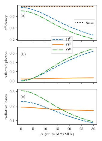
Figure 8: (a) Storage efficiency, (b) probability of photon reflection, Eq. (17), and (c) probability of spontaneous decay, Eq. (18), as a function of the single photon detuning $\Delta$ and at time $t_{2}$. The parameters are $(g,\kappa,\gamma)=(4.9,2.42,3.03)\times 2\pi\,\mathrm{MHz}$, $T_{\mathrm{c}}=0.5\,\mathrm{\mu s}$. The input photon $\mathcal{E}_{\mathrm{in}}(t)$ is defined as in Eq. (7). See Fig. 2 for further details.

The protocol $\Omega^{\mathrm{G}}(t)$ does not have any restriction on $\Delta$: for every $\Delta$ there is a pulse $\Omega^{\mathrm{G}}(t)$ that allows for storage with efficiency $\eta_{\mathrm{max}}$ (within the adiabatic regime), see Eq. (25). Figure 8 displays the storage efficiency and the losses for each protocol as a function of $\Delta$, as expected the protocol $\Omega^{\mathrm{G}}(t)$ performs in the same way for any values of $\Delta$.

A time-dependent phase $\chi(t)$ of the control pulse $\Omega(t)=|\Omega(t)|e^{\mathrm{i}\chi(t)}$ can be implemented as a two-photon detuning

$$\delta=\dot{\chi}(t).$$ (41)

In fact, by applying the unitary transformation $\hat{U}(t)=\exp\left(-\mathrm{i}\left|r\middle>\!\middle<r\right|\chi(t)\right)$, the transformed Hamiltonian is $\hat{H}^{\prime}=\hat{H}^{\prime}_{\mathrm{I}}+\hat{H}_{\mathrm{fields}}$, where

$$\hat{H}^{\prime}_{\mathrm{I}}={} \dot{\chi}(t)\left|r\middle>\!\middle<r\right|-\Delta\left|e\middle>\!\middle<e\right|+{}$$ (42)

$${}+\left(g\left|e\middle>\!\middle<g\right|\hat{a}+|\Omega(t)|\left|e\middle>\!\middle<r\right|+\mathrm{H.c.}\right).$$

For $\Omega^{\mathrm{G}}(t)$ we have

$$\dot{\chi}^{\mathrm{G}}(t) =\frac{-\Delta}{2\gamma(1+C)}\cdot\frac{|\mathcal{E}_{\mathrm{in}}(t)|^{2}}{\int_{t_{1}}^{t}|\mathcal{E}_{\mathrm{in}}(t^{\prime})|^{2}\det^{\prime}}=$$ (43a)

$$=\frac{-\Delta|\Omega^{\mathrm{G}}(t)|^{2}}{\Delta^{2}+\gamma^{2}(1+C)^{2}}\,.$$ (43b)

Recall that also $|\Omega^{\mathrm{G}}(t)|$ depends on $\Delta$. This can be understood in terms of AC Stark shift: one-photon detuning $\Delta\neq 0$ is a shift of the control laser out of resonance for the transition $|r\rangle-|e\rangle$ and thereby induces an AC Stark shift on the levels $|e\rangle$ and $|r\rangle$ of the atom; thus the condition of two-photon resonance does not hold anymore. In order to restore the latter, changes in frequency of the carrier and/or of the cavity and/or of the atomic levels are needed and they appear as a two-photon detuning in the Hamiltonian. This also explains why the reflected photon probability for the protocols $\Omega^{\mathrm{F}}(t)$ and $\Omega^{\mathrm{D}}(t)$ (see Fig. 8), which do not take into account the one-photon detuning, increases with increasing $\Delta$: the input photon sees the system out of resonance and hence it is mostly reflected.

Eq. (43b) gives the energy shift as a function of the Rabi frequency of the control pulse.

References

- (1) J. I. Cirac, P. Zoller, H. J. Kimble, and H. Mabuchi, Phys. Rev. Lett. 78, 3221 (1997).
- (2) H. J. Kimble, Nature 453, 1023 (2008).
- (3) M. Afzelius, N. Gisin, and Hu. de Riedmatten, Physics Today 68, 42 (2015).
- (4) K. Heshami, D. G. England, P. C. Humphreys, P. J. Bustard, V. M. Acosta, J. Nunn, B. J. Sussman, Journal of Modern Optics 63, S42-S65 (2016).
- (5) A. Kalachev, Phys. Rev. A 76, 043812 (2007).
- (6) A. Kalachev, Phys. Rev. A 78, 043812 (2008).
- (7) A. Kalachev, Opt. Spectrosc. 109, 32 (2010).
- (8) L.-M. Duan and C. Monroe, Rev. Mod. Phys. 82, 1209 (2010).
- (9) A. Reiserer and G. Rempe, Rev. Mod. Phys. 87, 1379 (2015).
- (10) C. Kurz, M. Schug, P. Eich, J. Huwer, P. Müller, and J. Eschner, Nat. Commun. 5, 5527 (2014).
- (11) S. Ritter, C. Nölleke, C. Hahn, A. Reiserer, A. Neuzner, M. Uphoff, M. Mücke, E. Figueroa, J. Bochmann, and G. Rempe, Nature 484, 195-200 (2012).
- (12) N. Kalb, A. Reiserer, S. Ritter, and G. Rempe, Phys. Rev. Lett. 114, 220501 (2015).
- (13) C. Kurz, P. Eich, M. Schug, P. Müller, and J. Eschner, Phys. Rev. A 93, 062348 (2016).
- (14) J. Brito, S. Kucera, P. Eich, P. Müller, and J. Eschner, Appl. Phys. B 122, 36 (2016).
- (15) M. Körber, O. Morin, S. Langenfeld, A. Neuzner, S. Ritter, and G. Rempe, Nat. Phot. 12, 18-21 (2018).
- (16) A. V. Gorshkov, A. André, M Fleischhauer, A. S. S Sørensen, and M. D. Lukin Phys. Rev. Lett. 98, 123601(2007).
- (17) M. Fleischhauer, S.F. Yelin, and M.D. Lukin, Opt. Commun. 179, 395 (2000).
- (18) J. Dilley, P. Nisbet-Jones, B. W. Shore, and A. Kuhn, Phys. Rev. A 85, 023834 (2012).
- (19) A. V. Gorshkov, A. André, M. D. Lukin, and A. S. Sørensen, Phys. Rev. A 76, 033804 (2007).
- (20) H. J. Carmichael, An open system approach to quantum optics, Springer-Verlag (Berlin, 1993).
- (21) S. Blum, G. A. Olivares-Rentería, C. Ottaviani, C. Becher, and G. Morigi, Phys. Rev. A 88, 053807 (2013).
- (22) P. Müller, T. Tentrup, M. Bienert, G. Morigi, and J. Eschner, Phys. Rev. A 96, 023861 (2017).
- (23) D. F. Walls and G. J. Milburn, Quantum Optics (Springer, Heidelberg, 1994).
- (24) A. V. Gorshkov, A. André, M. D. Lukin, and A. S. Sørensen, Phys. Rev. A 76, 033805 (2007).
- (25) J. Dalibard, Y. Castin, and K. Mølmer, Phys. Rev. Lett. 68, 580 (1992).
- (26) G. S. Vasilev, D. Ljunggren, and A. Kuhn, New J. Phys. 12, 063024 (2010).
- (27) M. Keller, B. Lange, K. Hayasaka, W. Lange, and H. Walther, New J. Phys. 6, 95 (2004).
- (28) P. B. R. Nisbet-Jones, J. Dilley, D. Ljunggren, and A. Kuhn, New J. Phys. 13, 103036 (2011).
- (29) I. Novikova, A. V. Gorshkov, D. F. Phillips, A. S. S Sørensen, M. D. Lukin, and R. L. Walsworth, Phys. Rev. Lett. 98, 243602 (2007).
- (30) A. V. Gorshkov, T. Calarco, M. D. Lukin, and A. S. Sørensen, Phys. Rev. A 77, 043806 (2008).
- (31) N. Khaneja, T. Reiss, C. Kehlet, T. Schulte-Herbrüggen, and S. J. Glaser, Journ. Magn. Res. 172(2), 296 (2005).
-
(32)
J. R. Johansson, P. D. Nation, and F. Nori, Comp.
Phys. Comm. 183, 1760 (2012).
J. R. Johansson, P. D. Nation, and F. Nori, Comp. Phys. Comm. 184, 1234 (2013).
J. R. Johansson, et al. Zenodo, qutip/qutip: QuTiP 4.2.0 (Version v4.2.0). http://doi.org/10.5281/zenodo.835881, (2017). - (33) C. P. Koch, J. Phys.: Condens. Matter 28, 213001 (2016).
- (34) C. Cohen-Tannoudji, J. Dupont-Roc, and G. Grynberg, Atom-Photon Interactions, (Wiley-VCH, 2004).