A Strong Stability Preserving Analysis for Explicit Multistage Two-Derivative Time-Stepping Schemes Based on Taylor Series Conditions.

Abstract

High order strong stability preserving (SSP) time discretizations are often needed to ensure the nonlinear (and sometimes non-inner-product) strong stability properties of spatial discretizations specially designed for the solution of hyperbolic PDEs. Multiderivative time-stepping methods have recently been increasingly used for evolving hyperbolic PDEs, and the strong stability properties of these methods are of interest. In our prior work we explored time discretizations that preserve the strong stability properties of spatial discretizations coupled with forward Euler and a second derivative formulation. However, many spatial discretizations do not satisfy strong stability properties when coupled with this second derivative formulation, but rather with a more natural Taylor series formulation. In this work we demonstrate sufficient conditions for an explicit two-derivative multistage method to preserve the strong stability properties of spatial discretizations in a forward Euler and Taylor series formulation. We call these strong stability preserving Taylor series (SSP-TS) methods. We also prove that the maximal order of SSP-TS methods is $p=6$, and define an optimization procedure that allows us to find such SSP methods. Several types of these methods are presented and their efficiency compared. Finally, these methods are tested on several PDEs to demonstrate the benefit of SSP-TS methods, the need for the SSP property, and the sharpness of the SSP time-step in many cases.

1 Introduction

The solution to a hyperbolic conservation law

$$U_{t}+f(U)_{x}=0,$$ (1)

may develop sharp gradients or discontinuities, which results in significant challenges to the numerical simulation of such problems. To ensure that it can handle the presence of a discontinuity, a spatial discretization is carefully designed to satisfy some nonlinear stability properties, often in a non-inner-product sense, e.g. total variation diminishing, maximum norm preserving, or positivity preserving properties. The development of high order spatial discretizations that can handle discontinuities is a major research area [6, 16, 29, 31, 36, 47, 48, 49, 4, 50, 55].

When the partial differential equation (1) is semi-discretized we obtain the ordinary differential equation (ODE)

$$u_{t}=F(u),$$ (2)

(where $u$ is a vector of approximations to $U$). This formulation is often referred to as a method of lines (MOL) formulation, and has the advantage of decoupling the spatial and time-discretizations. The spatial discretizations designed to handle discontinuities ensure that when the semi-discretized equation (2) is evolved using a forward Euler method

$$u^{n+1}=u^{n}+\Delta tF(u^{n}),$$ (3)

(where $u^{n}$ is a discrete approximation to $U$ at time $t^{n}$) the numerical solution satisfies the desired strong stability property, such as total variation stability or positivity. If the desired nonlinear stability property such as a norm, semi-norm, or convex functional, is represented by $\|\cdot\|$, the spatial discretization satisfies the monotonicity property

$$\|u^{n}+\Delta tF(u^{n})\|\leq\|u^{n}\|,$$ (4)

under the time-step restriction

$$0\leq\Delta t\leq\Delta t_{FE}.$$ (5)

In practice, in place of the first order time discretization (3), we typically require a higher-order time integrator, that preserves the strong stability property

$$\|u^{n+1}\|\leq\|u^{n}\|,$$ (6)

perhaps under a modified time-step restriction. For this purpose, time-discretizations with good linear stability properties or even with nonlinear inner-product stability properties are not sufficient. Strong stability preserving (SSP) time-discretizations were developed to address this need. SSP multistep and Runge–Kutta methods satisfy the strong stability property (6) for any function $F$, any initial condition, and any convex functional $\|\cdot\|$ under some time-step restriction, provided only that (4) is satisfied.

Recently, there has been interest in exploring the SSP properties of multiderivative Runge–Kutta methods, also known as multistage multiderivative methods. Multiderivative Runge–Kutta (MDRK) methods were first considered in [34, 52, 46, 41, 42, 22, 23, 32, 35, 3], and later explored for use with partial differential equations (PDEs) [40, 51, 30, 37, 9]. These methods have a form similar to Runge–Kutta methods but use an additional derivative $\dot{F}=u_{tt}\approx U_{tt}$ to allow for higher order. The SSP properties of these methods were discussed in [5, 33]. In [5], a method is defined as SSP-SD if it satisfies the strong stability property (6) for any function $F$, any initial condition, and any convex functional $\|\cdot\|$ under some time-step restriction, provided that (4) is satisfied for any $\Delta t\leq\Delta t_{FE}$ and an additional condition of the form

$$\|u^{n}+\Delta t^{2}\tilde{F}(u^{n})\|\leq\|u^{n}\|$$

is satisfied for any $\Delta t\leq\tilde{K}\Delta t_{FE}$. These conditions allow us to find a wide variety of time-discretizations, called SSP-SD time-stepping methods, but they limit the type of spatial discretization that can be used in this context.

In this paper, we present a different approach to the SSP analysis, which is more along the lines of the idea in [33]. For this analysis, we use, as before, the forward Euler base condition (4), but add to it a Taylor series condition of the form

$$\|u^{n}+\Delta tF(u^{n})+\frac{1}{2}\Delta t^{2}\tilde{F}(u^{n})\|\leq\|u^{n}\|$$

that holds for any $\Delta t\leq K\Delta t_{FE}$. Compared to those studied in [5], this pair of base conditions allows for more flexibility in the choice of spatial discretizations (such as the methods that satisfy a Taylor series condition in [10, 38, 7, 40]), at the cost of more limited variety of time discretizations. We call the methods that preserve the strong stability properties of these base conditions strong stability preserving Taylor series (SSP-TS) methods. The goal of this paper is to study a class of methods that is suitable for use with existing spatial discretizations, and present families of such SSP-TS methods that are optimized for the relationship between the forward-Euler time-step $\Delta t_{\textup{FE}}$ and the Taylor series timestep $K\Delta t_{FE}$.

In the following subsections we describe SSP Runge–Kutta time discreizations and present explicit multistage two-derivative methods. We then motivate the need for methods that preserve the nonlinear stability properties of the forward Euler and Taylor series base conditions. In Section 2 we formulate the SSP optimization problem for finding explicit two-derivative methods which can be written as the convex combination of forward Euler and Taylor series steps with the largest allowable time-step, which we will later use to find optimized methods. In Subsection 2.1 we explore the relationship between SSP-SD methods and SSP-TS methods. In Subsection 2.2 we prove that there are order barriers associated with explicit two-derivative methods that preserve the properties of forward Euler and Taylor series steps with a positive time-step. In Section 3 we present the SSP coefficients of the optimized methods we obtain. The methods themselves can be downloaded from our github repository [14]. In Section 4 we demonstrate how these methods perform on specially selected test cases, and in Section 5 we present our conclusions.

1.1 SSP methods

It is well-known [43, 13] that some multistep and Runge–Kutta methods can be decomposed into convex combinations of forward Euler steps, so that any convex functional property satisfied by (4) will be preserved by these higher-order time discretizations. If we re-write the $s$-stage explicit Runge–Kutta method in the Shu-Osher form [44],

$$y^{(0)} = u^{n},$$

$$y^{(i)} = \sum_{j=0}^{i-1}\left(\alpha_{i,j}y^{(j)}+\Delta t\beta_{i,j}F(y^{(j)})\right),\;\;\;\;i=1,...,s$$ (7)

$$u^{n+1} = y^{(s)}$$

it is clear that if all the coefficients $\alpha_{i,j}$ and $\beta_{i,j}$ are non-negative, and provided $\alpha_{i,j}$ is zero only if its corresponding $\beta_{i,j}$ is zero, then each stage can be written as a convex combination of forward Euler steps of the form (3), and be bounded by:

$$\|y^{(i)}\| = \left\|\sum_{j=0}^{i-1}\left(\alpha_{i,j}y^{(j)}+\Delta t\beta_{i,j}F(y^{(j)})\right)\right\|$$

$$\leq \sum_{j=0}^{i-1}\alpha_{i,j}\,\left\|y^{(j)}+\Delta t\frac{\beta_{i,j}}{\alpha_{i,j}}F(y^{(j})\right\|\leq\sum_{j=0}^{i-1}\alpha_{i,j}\,\left\|y^{(j)}\right\|$$

under the condition $\frac{\beta_{i,j}}{\alpha_{i,j}}\Delta t\leq\Delta t_{\textup{FE}}$. By the consistency condition $\sum_{j=0}^{i-1}\alpha_{i,j}=1$, we now have $\|u^{n+1}\|\leq\|u^{n}\|$, under the condition

$$\Delta t\leq{\cal{C}}\Delta t_{\textup{FE}}\;\;\;\;\mbox{where}\;\;{\cal{C}}=\min_{i,j}\frac{\alpha_{i,j}}{\beta_{i,j}}$$ (8)

where if any of the $\beta$s are equal to zero, the corresponding ratios are considered infinite.

If a method can be decomposed into such a convex combination of (3), with a positive value of ${\cal{C}}>0$ then the method is called strong stability preserving (SSP), and the value ${\cal{C}}$ is called the SSP coefficient. SSP methods guarantee the strong stability properties of any spatial discretization, provided only that these properties are satisfied when using the forward Euler method. The convex combination approach guarantees that the intermediate stages in a Runge–Kutta method satisfy the desired strong stability property as well. The convex combination approach clearly provides a sufficient condition for preservation of strong stability. Moreover, it has also be shown that this condition is necessary [11, 12, 17, 18].

Second and third order explicit Runge–Kutta methods [44] and later fourth order methods [45, 24] were found that admit such a convex combination decomposition with ${\cal{C}}>0$. However, it has been proven that explicit Runge–Kutta methods with positive SSP coefficient cannot be more than fourth-order accurate [28, 39].

The time-step restriction (8) is comprised of two distinct factors: (1) the term $\Delta t_{\textup{FE}}$ that is a property of the spatial discretization, and (2) the SSP coefficient ${\cal{C}}$ that is a property of the time-discretization. Research on SSP time-stepping methods for hyperbolic PDEs has primarily focused on finding high-order time discretizations with the largest allowable time-step $\Delta t\leq{\cal{C}}\Delta t_{\textup{FE}}$ by maximizing the SSP coefficient ${\cal{C}}$ of the method.

High order methods can also be obtained by adding more steps (e.g. linear multistep methods) or more derivatives (Taylor series methods). Multistep methods that are SSP have been found [13], and explicit multistep SSP methods exist of very high order $p>4$, but have severely restricted SSP coefficients [13]. These approaches can be combined with Runge–Kutta methods to obtain methods with multiple steps, and stages. Explicit multistep multistage methods that are SSP and have order $p>4$ have been developed as well [25, 1].

1.2 Explicit Multistage two-derivative methods

Another way to obtain higher order methods is to use higher derivatives combines with the Runge–Kutta approach. An explicit multistage two-derivative time integrator is given by:

$$y^{(i)} = u^{n}+\Delta t\sum_{j=1}^{i-1}a_{ij}F(y^{(j)})+\Delta t^{2}\sum_{j=1}^{i-1}\hat{a}_{ij}\dot{F}(y^{(j)}),\;\;\;\;i=2,...,s$$ (9)

$$u^{n+1} = u^{n}+\Delta t\sum_{j=1}^{s}b_{j}F(y^{(j)})+\Delta t^{2}\sum_{j=1}^{i-1}\hat{b}_{j}\dot{F}(y^{(j)}),$$

where $y^{(1)}=u^{n}$.

The coefficients can be put into matrix vector form, where

$$A=\left(\begin{array}[]{llll}0&0&\vdots&0\\ a_{21}&0&\vdots&0\\ \vdots&\vdots&\vdots&\vdots\\ a_{s1}&a_{s2}&\vdots&0\\ \end{array}\right),\;\;\hat{A}=\left(\begin{array}[]{llll}0&0&\vdots&0\\ \hat{a}_{21}&0&\vdots&0\\ \vdots&\vdots&\vdots&\vdots\\ \hat{a}_{s1}&\hat{a}_{s2}&\vdots&0\\ \end{array}\right),\;\;b=\left(\begin{array}[]{llll}b_{1}\vspace{0.1in}\\ b_{2}\vspace{0.1in}\\ \vdots\\ b_{s}\vspace{0.1in}\\ \end{array}\right),\;\;\hat{b}=\left(\begin{array}[]{llll}\hat{b}_{1}\vspace{0.1in}\\ \hat{b}_{2}\vspace{0.1in}\\ \vdots\\ \hat{b}_{s}\vspace{0.1in}\\ \end{array}\right).$$

We also define the vectors $c=A{\bf e}$ and $\hat{c}=\hat{A}{\bf e}$, where ${\bf e}$ is a vector of ones.

As in our prior work [5], we focus on using explicit multistage two-derivative methods as time integrators for evolving hyperbolic PDEs. For our purposes, the operator $F$ is obtained by a spatial discretization of the term $U_{t}=-f(U)_{x}$ to obtain the system $u_{t}=F(u)$. Instead of computing the second derivative term $\dot{F}$ directly from the definition of the spatial discretization $F$, we approximate $\tilde{F}\approx\dot{F}$ by employing the Cauchy-Kowalevskaya procedure which uses the PDE (1) to replace the time derivatives by the spatial derivatives, and discretize these in space.

If the term $F(u)$ is computed using a conservative spatial discretization $D_{x}$ applied to the flux:

$$F(u)=-D_{x}(f(u)),$$ (10)

then we approximate the second derivative

$$\dot{F}(u)=u_{tt}\approx U_{tt}=-f(U)_{xt}=-\left(f(U)_{t}\right)_{x}=-\left(f^{\prime}(U)U_{t}\right)_{x}\approx-\tilde{D}_{x}\left(f^{\prime}(u)u_{t}\right)=\tilde{F}(u),$$ (11)

where a (potentially different) spatial differentiation operator $\tilde{D}_{x}$ is used. Although these two approaches are different, the differences between them are of high order in space, so that in practice, as long as the spatial errors are smaller than the temporal errors, we see the correct order of accuracy in time, as shown in [5].

1.3 Motivation for the new base conditions for SSP analysis

In [5] we considered explicit multistage two-derivative methods and developed sufficient conditions for a type of strong stability preservation for these methods. We showed that explicit SSP-SD methods within this class can break this well-known order barrier for explicit Runge–Kutta methods. In that work we considered two-derivative methods that preserve the strong stability property satisfied by a function $F$ under a convex functional $\|\cdot\|$, provided that the conditions:

$$\mbox{\bf Forward Euler condition:}\;\;\|u^{n}+\Delta tF(u^{n})\|\leq\|u^{n}\|\;\;\mbox{for}\;\;\Delta t\leq\Delta t_{FE},$$ (12)

and

$$\mbox{\bf Second derivative condition:}\;\;\|u^{n}+\Delta t^{2}\tilde{F}(u^{n})\|\leq\|u^{n}\|\;\;\mbox{for}\;\;\Delta t\leq\tilde{K}\Delta t_{FE},$$ (13)

where $\tilde{K}$ is a scaling factor that compares the stability condition of the second derivative term to that of the forward Euler term. While the forward Euler condition is characteristic of all SSP methods (and has been justified by the observation that it is the circle contractivity condition in [11]), the second derivative condition was chosen over the Taylor series condition:

$$\mbox{\bf Taylor series condition:}\;\;\|u^{n}+\Delta tF(u^{n})+\frac{1}{2}\Delta t^{2}\tilde{F}(u^{n})\|\leq\|u^{n}\|\;\;\mbox{for}\;\;\Delta t\leq K\Delta t_{FE},$$ (14)

because it is more general. If the forward Euler (12) and second derivative (13) conditions are both satisfied, then the Taylor series condition (14) will be satisfied as well. Thus, a spatial discretization that satisfies (12) and (13) will also satisfy (14), so that the SSP-SD concept in [5] allows for the most general time-discretizations. Furthermore, some methods of interest and importance in the literature cannot be written using a Taylor series decomposition, most notably the unique two-stage fourth order method

$$y^{(1)} = u^{n}+\frac{1}{2}\Delta tF(u^{n})+\frac{1}{8}\Delta t^{2}\dot{F}(u^{n})$$ (15a)

$$u^{n+1} = u^{n}+\Delta tF(u^{n})+\frac{1}{6}\Delta t^{2}\dot{F}(u^{n})+\frac{1}{3}\Delta t^{2}\dot{F}(y^{(1)})$$ (15b)

which appears commonly in the literature on this subject [30, 37, 9]. For these reasons, it made sense to first consider the SSP-SD property which relies on the pair of base conditions (12) and (13).

However, as we will see in the example below, there are spatial discretizations for which the second derivative condition (13) is not satisfied but the forward Euler condition (12) and the Taylor series condition (14) are both satisfied. In such cases, the SSP-SD methods derived in [5] may not preserve the desired strong stability properties. The existence of such spatial discretizations is the main motivation for the current work, in which we re-examine the strong stability properties of the explicit two-derivative multistage method (9) using the base conditions (12) and (14). Methods that preserve the strong stability properties of (12) and (14) are called herein SSP-TS methods. The SSP-TS approach increases our flexibility in the choice of spatial discretization over the SSP-SD approach. Of course, this enhanced flexibility in the choice of spatial discretization is expected to result in limitations on the time-discretization (e.g. the two-stage fourth order method is SSP-SD but not SSP-TS).

To illustrate the need for time-discretizations that preserve the strong stability properties of spatial discretizations that satisfy (12) and (14), but not (13), consider the one-way wave equation

$$U_{t}=U_{x}$$

(here $f(U)=U$) where $F$ is defined by the first-order upwind method

$$F(u^{n})_{j}:=\frac{1}{\Delta x}\left(u^{n}_{j+1}-u^{n}_{j}\right)\approx U_{x}(x_{j}).$$ (16)

When solving the PDE, we compute the operator $\tilde{F}$ by simply applying the differentiation operator twice (note that $f^{\prime}(U)=1$)

$$\dot{F}\approx\tilde{F}:=\frac{1}{\Delta x^{2}}\left(u^{n}_{j+2}-2u^{n}_{j+1}+u^{n}_{j}\right).$$ (17)

We note that when computed this way, the spatial discretization $F$ coupled with forward Euler satisfies the total variation diminishing (TVD) condition:

$$\|u^{n}+\Delta tF(u^{n})\|_{TV}\leq\|u^{n}\|_{TV}\;\;\;\;\mbox{for}\;\;\;\;\Delta t\leq\Delta x,$$ (18)

while the Taylor series term using $F$ and $\tilde{F}$ satisfies the TVD

$$\|u^{n}+\Delta tF(u^{n})+\frac{1}{2}\Delta t^{2}\tilde{F}(u^{n})\|_{TV}\leq\|u^{n}\|_{TV}\;\;\;\;\mbox{for}\;\;\;\;\Delta t\leq\Delta x.$$ (19)

In other words, these spatial discretizations satisfy the conditions (12) and (14) with $K=1$, in the total variation semi-norm. However, (13) is not satisfied, so the methods derived in [5] cannot be used. Our goal in the current work is to develop time discretizations that will preserve the desired strong stability properties (e.g. the total variation diminishing property) when using spatial discretizations such as the upwind approximation (17) that satisfy (12) and (14) but not (13).

Remark 1.

This simple first order motivating example is chosen because these spatial discretizations are provably TVD and allow us to see clearly why the Taylor series base condition (14) is needed. In practice, we use higher order spatial discretizations such as WENO that do not have a theoretical guarantee of TVD, but perform well in practice. Such methods are considered in Examples 2 and 4 in the numerical tests, and provide us with similar results.

In this work we develop explicit two-derivative multistage SSP-TS methods of the form (9) that preserve the convex functional properties of forward Euler and Taylor series terms. When the spatial discretizations $F$ and $\tilde{F}$ that satisfy (12) and (14) are coupled with such a time-stepping method, the strong stability condition

$$\|u^{n+1}\|\leq\|u^{n}\|$$

will be preserved, perhaps under a different time-step condition

$$\Delta t\leq{\cal{C}}_{TS}\Delta t_{\textup{FE}}.$$ (20)

If a method can be decomposed in such a way, with ${\cal{C}}_{TS}>0$ we say that it is SSP-TS. In the next section, we define an optimization problem that will allow us to find SSP-TS methods of the form (9) with the largest possible SSP coefficient ${\cal{C}}_{TS}$.

2 SSP Explicit Two-Derivative Runge–Kutta Methods

We consider the system of ODEs

$$u_{t}=F(u)$$ (21)

resulting from a semi-discretization of the hyperbolic conservation law (1) such that $F$ satisfies the forward Euler (first derivative) condition (12)

$$\mbox{\bf Forward Euler condition:}\;\;\|u^{n}+\Delta tF(u^{n})\|\leq\|u^{n}\|\;\;\mbox{for}\;\;\Delta t\leq\Delta t_{FE},$$

for the desired stability property indicated by the convex functional $\|\cdot\|$.

The methods we are interested in also require an appropriate approximation to the second derivative in time

$$\tilde{F}\approx\dot{F}=u_{tt}.$$

We assume in this work that $F$ and $\tilde{F}$ satisfy an additional condition of the form (14)

$$\mbox{\bf Taylor series condition:}\;\;\|u^{n}+\Delta tF(u^{n})+\frac{1}{2}\Delta t^{2}\tilde{F}(u^{n})\|\leq\|u^{n}\|\;\;\mbox{for}\;\;\Delta t\leq K\Delta t_{FE},$$

in the same convex functional $\|\cdot\|$, where $K$ is a scaling factor that compares the stability condition of the Taylor series term to that of the forward Euler term.

We wish to show that given conditions (12) and (14), the multi-derivative method (9) satisfies the desired monotonicity condition under a given time-step. This is easier if we re-write the method (9) in an equivalent matrix-vector form

$${\bf y}={\bf e}u^{n}+\Delta tSF({\bf y})+\Delta t^{2}\hat{S}\tilde{F}({\bf y}),$$ (22)

where ${\bf y}=\left(y^{(1)},y^{(2)},...,y^{(s)},u^{n+1}\right)^{T}$,

$$S=\left[\begin{array}[]{ll}A&\textbf{0}\\ b^{T}&0\end{array}\right]\;\;\;\;\;\mbox{and}\;\;\;\;\;\hat{S}=\left[\begin{array}[]{ll}\hat{A}&\textbf{0}\\ \hat{b}^{T}&0\end{array}\right]$$

and ${\bf e}$ is a vector of ones. As in prior SSP work, all the coefficients in $S$ and $\hat{S}$ must be non-negative (see Lemma 3).

We can now easily establish sufficient conditions for an explicit method of the form (22) to be SSP:

Theorem 1.

Given spatial discretizations $F$ and $\tilde{F}$ that satisfy (12) and (14), an explicit two-derivative multistage method of the form (22) preserves the strong stability property $\|u^{n+1}\|\leq\|u^{n}\|$ under the time-step restriction $\Delta t\leq r\Delta t_{\textup{FE}}$ if it satisfies the conditions

$$\left(I+rS+\frac{2r^{2}}{K^{2}}\left(1-K\right)\hat{S}\right)^{-1}{\bf e}\geq 0$$ (23a)

$$r\left(I+rS+\frac{2r^{2}}{K^{2}}\left(1-K\right)\hat{S}\right)^{-1}\left(S-\frac{2r}{K}\hat{S}\right)\geq 0$$ (23b)

$$\frac{2r^{2}}{K^{2}}\left(I+rS+\frac{2r^{2}}{K^{2}}\left(1-K\right)\hat{S}\right)^{-1}\hat{S}\geq 0$$ (23c)

for some $r>0$. In the above conditions, the inequalities are understood component-wise.

Proof.

We begin with the method

$${\bf y}={\bf e}u^{n}+\Delta tSF({\bf y})+\Delta t^{2}\hat{S}\tilde{F}({\bf y}),$$

and add the terms $rS{\bf y}$ and $2\hat{r}(\hat{r}-r)\hat{S}{\bf y}$ to both sides to obtain the canonical Shu-Osher form of an explicit two-derivative multistage method:

$$\left(I+rS+2\hat{r}(\hat{r}-r)\hat{S}\right){\bf y} = u^{n}{\bf e}+r(S-2\hat{r}\hat{S})\left({\bf y}+\frac{\Delta t}{r}F({\bf y})\right)$$

$$+2\hat{r}^{2}\hat{S}\left({\bf y}+\frac{\Delta t}{\hat{r}}F({\bf y})+\frac{\Delta t^{2}}{2\hat{r}^{2}}\tilde{F}({\bf y})\right),$$

$${\bf y} = R({\bf e}u^{n})+P\left({\bf y}+\frac{\Delta t}{r}F({\bf y})\right)+Q\left({\bf y}+\frac{\Delta t}{\hat{r}}F({\bf y})+\frac{\Delta t^{2}}{2\hat{r}^{2}}\tilde{F}({\bf y})\right),$$

where

$$R=\left(I+rS+2\hat{r}(\hat{r}-r)\hat{S}\right)^{-1},\;\;\;\;\;\;P=rR\left(S-2\hat{r}\hat{S}\right),\;\;\;\;\;\;Q=2\hat{r}^{2}R\hat{S}.$$

If the elements of $P$, $Q$, and $R{\bf e}$ are all non-negative, and if $\left(R+P+Q\right){\bf e}={\bf e}$, then ${\bf y}$ is a convex combination of strongly stable terms

$$\|{\bf y}\|\leq R\|{\bf e}u^{n}\|+P\|{\bf y}+\frac{\Delta t}{r}F({\bf y})\|+Q\|{\bf y}+\frac{\Delta t}{\hat{r}}F({\bf y})+\frac{\Delta t^{2}}{2\hat{r}^{2}}\tilde{F}({\bf y})\|,$$

and so is also strongly stable under the time-step restrictions $\Delta t\leq r\Delta t_{\textup{FE}}$ and $\Delta t\leq K\hat{r}\Delta t_{\textup{FE}}$. In such cases, the optimal time-step is given by the minimum of the two. In the cases we encounter here, this minimum occurs when these two values are set equal, so we require $r=K\hat{r}$. Conditions (23a)–(23c) now ensure that $P\geq 0$, $Q\geq 0$, and $R{\bf e}\geq 0$ component-wise for $\hat{r}=\frac{r}{K}$, and so the method preserves the strong stability condition $\|u^{n+1}\|\leq\|u^{n}\|$ under the time-step restriction $\Delta t\leq r\Delta t_{FE}$. Note that if this fact holds for a given value of $r>0$ then it also holds for all smaller positive values. ∎

Definition 1.

A method that satisfies the conditions in Theorem 1 for values $r\in(0,r_{max}]$ is called a Strong Stability Preserving Taylor Series (SSP-TS) method with an associated SSP coefficient

$${\cal{C}}_{TS}=r_{max}.$$

Remark 2.

Theorem 1 gives us the conditions for the method (22) to be SSP-TS for any time-step $\Delta t\leq{\cal{C}}_{TS}\Delta t_{\textup{FE}}$. We note, however, that while the corresponding conditions for Runge–Kutta methods have been shown to be necessary as well as sufficient, for the multi-derivative methods we only show that these conditions are sufficient. This is a consequence of the fact that we define this notion of SSP based on the conditions (12) and (14), but if a spatial discretization also satisfies a different condition (for example, (13)) many other methods of the form (22) also give strong stability preserving results. Notable among these is the two-derivative two-stage fourth order method (15) which is SSP-SD but not SSP-TS. This means that solutions of (15) can be shown to satisfy the strong stability property $\|u^{n+1}\|\leq\|u^{n}\|$ for positive time-steps, for the appropriate spatial discretizations, even though the conditions in Theorem 1 are not satisfied.

This result allows us to formulate the search for optimal SSP-TS methods as an optimization problem, as in [5, 13, 24, 26]

Find the coefficient matrices $S$ and $\hat{S}$
that maximize the value of ${\cal{C}}_{TS}=\max r$
such that the relevant order conditions (summarized in Appendix A)
and the SSP conditions (23a)-(23c) are all satisfied.

However, before we present the optimal methods in Section 3, we present the theoretical results on the allowable order of multistage multi-derivative SSP-TS methods.

2.1 SSP results for explicit two-derivative Runge–Kutta methods

In this paper, we consider explicit SSP-TS two-derivative multistage methods that can be decomposed into a convex combination of (12) and (14), and thus preserve their strong stability properties. In our previous work [5] we studied SSP-SD methods of the form (9) that can be written as convex combinations of (12) and (13). The following lemma explains the relationship between these two notions of strong stability.

Lemma 1.

Any explicit method of the form (9) that can be written as a convex combination of the forward Euler formula (12) and the Taylor series formula (14) can also be written as a convex combination of the forward Euler formula (12) and the second derivative formula (13).

Proof.

We can easily see that any Taylor series step can be rewritten as a convex combination of the forward Euler formula (12) and the second derivative formula (13):

$$u^{n}+\Delta tF(u^{n})+\frac{1}{2}\Delta t^{2}\tilde{F}(u^{n})=\alpha\left(u^{n}+\frac{\Delta t}{\alpha}F(u^{n})\right)+(1-\alpha)\left(u^{n}+\frac{1}{2(1-\alpha)}\Delta t^{2}\tilde{F}(u^{n})\right),$$

for any $0<\alpha<1$. Clearly then, if a method can be decomposed into a convex combination of (12) and (14), and in turn (14) can be decomposed into a convex combination of (12) and (13), then the method itself can be written as a convex combination of (12) and (13). ∎

This result recognizes that the SSP-TS methods we study in this paper are a subset of the SSP-SD methods in [5]. This allows us to use results about SSP-SD methods when studying the properties of SSP-TS methods.

The following lemma establishes the Shu-Osher form of an SSP-SD method of the form (9). This form allows us to directly observe the convex combination of steps of the form (12) and (13), and thus easily identify the SSP coefficient ${\cal{C}}_{SD}$.

Lemma 2.

If an explicit method of the form (9) written in the Shu-Osher form

$$y^{(1)} = u^{n}$$

$$y^{(i)} = \sum_{j=1}^{i-1}\alpha_{ij}y^{(j)}+\Delta t\beta_{ij}F(y^{(j)})+\hat{\alpha}_{ij}y^{(j)}+\Delta t^{2}\hat{\beta}_{ij}\tilde{F}(y^{(j)}),\;\;\;\;i=2,...,s+1$$ (24)

$$u^{n+1} = y^{(s+1)}$$

has the properties that

1. all the coefficients are non-negative,

2. $\beta_{ij}=0$ whenever $\alpha_{ij}=0$

3. $\hat{\beta}_{ij}=0$ whenever $\hat{\alpha}_{ij}=0$

then this method preserves the strong stability properties of (12) and (13) (i.e. is SSP-SD) for $\Delta t\leq{\cal{C}}_{SD}\Delta t_{\textup{FE}}$ with

$${\cal{C}}_{SD}=\min_{i,j}\left\{\frac{\alpha_{i,j}}{\beta_{i,j}},\tilde{K}\frac{\hat{\alpha}_{ij}}{\hat{\beta}_{ij}}\right\}$$

.

Proof.

For each stage we have

$$\|y^{(i)}\| = \left\|\sum_{j=1}^{i-1}\alpha_{ij}y^{(j)}+\Delta t\beta_{ij}F(y^{(j)})+\hat{\alpha}_{ij}y^{(j)}+\Delta t^{2}\hat{\beta}_{ij}\tilde{F}(y^{(j)})\right\|$$

$$\leq \sum_{j=1}^{i-1}\alpha_{ij}\left\|y^{(j)}+\Delta t\frac{\beta_{ij}}{\alpha_{ij}}F(y^{(j)})\right\|+\sum_{j=1}^{i-1}\hat{\alpha}_{ij}\left\|y^{(j)}+\Delta t^{2}\frac{\hat{\beta}_{ij}}{\hat{\alpha}_{ij}}\tilde{F}(y^{(j)})\right\|$$

$$\leq \sum_{j=1}^{i-1}\left(\alpha_{ij}+\hat{\alpha}_{ij}\right)\|u^{n}\|$$

assuming only that for each one of these $\Delta t\frac{\beta_{ij}}{\alpha_{ij}}\leq\Delta t_{\textup{FE}}$ and $\Delta t\frac{\hat{\beta}_{ij}}{\hat{\alpha}_{ij}}\leq\tilde{K}\Delta t_{\textup{FE}}$. The result immediately follows from the fact that for each $i$ we have $\sum_{j=1}^{i-1}\left(\alpha_{ij}+\hat{\alpha}_{ij}\right)=1$ for consistency. ∎

When a method is written in the block Butcher form (22), we can decompose it into a canonical Shu-Osher form.

$$Y = (I+rS+\hat{r}\hat{S})^{-1}eu^{n}+(I+rS+\hat{r}\hat{S})^{-1}S(Y+\frac{\Delta t}{r}F(Y))+(I+rS+\hat{r}\hat{S})^{-1}\hat{S}(Y+\frac{\Delta t^{2}}{\hat{r}}\tilde{F}(Y)).$$

This allows us to define an SSP-SD method directly from the Butcher coefficients.

Definition 2.

Given spatial discretizations $F$ and $\tilde{F}$ that satisfy (12) and (13), an explicit two-derivative multistage method of the form (22) is called a Strong Stability Preserving Second Derivative (SSP-SD) method with and associated SSP coefficient ${\cal{C}}_{SD}=\min\{r_{max},\tilde{K}\hat{r}_{max}\}$ if it satisfies the conditions

$$(I+rS+\hat{r}\hat{S})^{-1}e \geq 0$$ (25a)

$$(I+rS+\hat{r}\hat{S})^{-1}rS \geq 0$$ (25b)

$$(I+rS+\hat{r}\hat{S})^{-1}\hat{r}\hat{S} \geq 0.$$ (25c)

for all $r=(0,r_{max}]$ and $\hat{r}=(0,\hat{r}_{max}]$. In the above conditions, the inequalities are understood component-wise.

The relationship between the coefficients in (9) and (2) allows us to conclude that the matrices $S$ and $\hat{S}$ must contain only non-negative coefficients.

Lemma 3.

If an explicit method of the form (9) can be converted to the Shu-Osher form (2) with all non-negative coefficients $\alpha_{ij},\beta_{ij},\hat{\alpha}_{ij},\hat{\beta}_{ij},$ for all $i,j$, then the coefficients $a_{ij},b_{j},\hat{a}_{ij},\hat{b}_{j}$ must be all non-negative as well.

Proof.

The transformation between (9) and (2) is given by $a_{21}=\beta_{21}$ and $\hat{a}_{21}=\hat{\beta}_{21}$ and, recursively,

$$a_{ij} = \beta_{ij}+\sum_{k=j+1}^{i-1}(\alpha_{ik}+\hat{\alpha}_{ik})a_{kj}$$ (26a)

$$\hat{a}_{ij} = \hat{\beta}_{ij}+\sum_{k=j+1}^{i-1}(\alpha_{ik}+\hat{\alpha}_{ik})\hat{a}_{kj}$$ (26b)

$$b_{j} = \beta_{s+1,j}+\sum_{k=j+1}^{s}(\alpha_{s+1,k}+\hat{\alpha}_{s+1,k})a_{kj}$$ (26c)

$$\hat{b}_{j} = \hat{\beta}_{s+1,j}+\sum_{k=j+1}^{s}(\alpha_{s+1,k}+\hat{\alpha}_{s+1,k})\hat{a}_{kj}$$ (26d)

Clearly then,

$$\beta_{21}\geq 0\implies a_{21}\geq 0$$

and

$$\hat{\beta}_{21}\geq 0\implies\hat{a}_{21}\geq 0.$$

From there we proceed recursively: Given that all $\alpha_{ij}\geq 0$ and $\beta_{ij}\geq 0$ for all $i,j$, and that $a_{kj}\geq 0$ and $\hat{a}_{kj}\geq 0$ for all $1\leq j<k\leq i-1$, then by the formulae (26a) and (26b) we have $a_{ij}\geq 0$ and $\hat{a}_{ij}\geq 0$.

Now given $\alpha_{ij}\geq 0$ and $\beta_{ij}\geq 0$ for all $i,j$ and $a_{kj}\geq 0$ and $\hat{a}_{kj}\geq 0$ for all $1\leq j<k\leq s$, the formulae (26c) and (26d) give the result $b_{j}\geq 0$ and $\hat{b}_{i}\geq 0$. Thus, all the coefficients $a_{ij},\hat{a}_{ij},b_{j},\hat{b}_{j}$ must be all non-negative.

∎

We wish to study only those methods for which the Butcher form (9) is unique. To do so, we follow Higueras [19] in extending the reducibility definition of Dahlquist and Jeltsch [20]. Other notions of reducibility exist, but for our purposes it is sufficient to define irreducibility as follows:

Definition 3.

A two-derivative multistage method of the form (9) is DJ-reducible if there exist sets $T_{1}$ and $T_{2}$ such that $T_{1}\neq\emptyset$, $T_{1}\bigcap T_{2}=\emptyset$, $T_{1}\bigcup T_{2}=[1,2,...,s]$, and

$$b_{j}=\hat{b}_{j}=0,\;\;\;\;j\in T_{1}$$

$$a_{ij}=\hat{a}_{ij}=0,\;\;\;\;i\in T_{1},\;j\in T_{2}.$$

We say a method is irreducible if it is not DJ-reducible.

Lemma 4.

An irreducible explicit SSP-SD method of the form (22) must satisfy the (componentwise) condition

$$b+\hat{b}>0.$$

Proof.

An SSP-SD method in the block form (22), must satisfy conditions (25a)–(25c) for $0<r\leq r_{max}$ and $0<\hat{r}\leq\hat{r}_{max}$. The non-negativity of (25b) and (25c) requires their sum to be non-negative as well,

$$(I+rS+\hat{r}\hat{S})^{-1}(rS+\hat{r}\hat{S})\geq 0.$$

Note that these matrices commute, so we have

$$(rS+\hat{r}\hat{S})(I+rS+\hat{r}\hat{S})^{-1}\geq 0.$$

Recalling the definition of the matrix $S$, we have

$$e_{s+1}(rS+\hat{r}\hat{S})(I+rS+\hat{r}\hat{S})^{-1}\geq 0$$

$$([(rb+\hat{r}\hat{b}),0])(I+rS+\hat{r}\hat{S})^{-1}\geq 0$$

Now, we can expand the inverse as

$$([(rb+\hat{r}\hat{b}),0])(I-(rS+\hat{r}\hat{S})+(rS+\hat{r}\hat{S})^{2}-(rS+\hat{r}\hat{S})^{3}+...)\geq 0$$

Because the positivity must hold for arbitrarily small $r<<1$ and $\hat{r}<<1$ we can stop our expansion after the linear term, and require

$$([(rb+\hat{r}\hat{b}),0])(I-(rS+\hat{r}\hat{S}))\geq 0,$$

which is

$$(rb+\hat{r}\hat{b})(I-(rA+\hat{r}\hat{A}))\geq 0\implies(rb+\hat{r}\hat{b})\geq(rb+\hat{r}\hat{b})(rA+\hat{r}\hat{A})).$$

Now we are ready to address the proof. Assume that $j=J$ is the largest value for which we have $b_{J}=\hat{b}_{J}=0$,

$$0=(rb+\hat{r}\hat{b})e_{J}\geq(rb+\hat{r}\hat{b})(rA+\hat{r}\hat{A})e_{J}\geq 0$$

Clearly, then we have

$$r\sum_{i}(rb_{i}+\hat{r}\hat{b}_{i})A_{iJ}+\hat{r}\sum_{i}(rb_{i}+\hat{r}\hat{b}_{i})\hat{A}_{iJ}=0$$

Since the method is explicit, the matrices $A$ and $\hat{A}$ are lower triangular (i.e $a_{iJ}=\hat{a}_{iJ}=0$ for $i\leq J$), so this condition becomes

$$r\sum_{i=J+1}^{s}(rb_{i}+\hat{r}\hat{b}_{i})A_{iJ}+\hat{r}\sum_{i=J+1}^{s}(rb_{i}+\hat{r}\hat{b}_{i})\hat{A}_{iJ}=0$$ (27)

By the assumption above, we have $(b_{i}+\hat{b}_{i})>0$ for $i>J$, and $r>0,\hat{r}>0$. Clearly, then, for (27) to hold we must require

$$A_{iJ}=\hat{A}_{iJ}=0\;\;\;\;\;\mbox{ for}\;\;\;\;i>J,$$

which, together with $b_{J}=\hat{b}_{J}=0$, makes the method DJ-reducible. Thus we have a contradiction. ∎

We note that this same result, in the context of additive Runge–Kutta methods, is due to Higueras [19].

2.2 Order barriers

Explicit SSP Runge–Kutta methods with ${\cal{C}}>0$ are known to have an order barrier of four, while the implicit methods have a barrier of six [13]. This follows from the fact that the order $p$ of irreducible methods with nonnegative coefficients depends on the stage order $q$ such that

$$q\geq\left\lfloor\frac{p-1}{2}\right\rfloor.$$

For explicit Runge–Kutta methods the first stage is a forward Euler step, so $q=1$ and thus $p\leq 4$, whereas for implicit Runge–Kutta methods the first stage is at most of order two, so that $q=2$ and thus $p\leq 6$.

For two-derivative multistage SSP-TS methods, we find that similar results hold. A stage order of $q=2$ is possible for explicit two-derivative methods (unlike explicit Runge–Kutta methods) because the first stage can be second order, i.e., a Taylor series method. However, since the first stage can be no greater than second order we have a bound on the stage order $q\leq 2$, which results in an order barrier of $p\leq 6$ for these methods. In the following results we establish these order barriers.

Lemma 5.

Given an irreducible SSP-TS method of the form (9), if $b_{j}=0$ then the corresponding $\hat{b}_{j}=0$.

Proof.

In any SSP-TS method the appearance of a second derivative term $\tilde{F}$ can only happen as part of a Taylor series term. This tells us that the $\tilde{F}$ must be accompanied by the corresponding $F$, meaning that whenever we have a nonzero $\hat{a}_{ij}$ or $\hat{b_{j}}$ term, the corresponding ${a}_{ij}$ or ${b_{j}}$ term must be nonzero. ∎

Lemma 6.

Any irreducible explicit SSP-TS method of the form (9) must satisfy the (componentwise) condition

$$b>0.$$

Proof.

Any irreducible method (9) that can be written as a convex combination of (12) and (14) can also be written as a convex combination of (12) and (13), according to Lemma 1. Applying Lemma 4 we obtain the condition $b+\hat{b}>0$, componentwise. Now, Lemma 5 tells us that if any component ${b}_{j}=0$ then its corresponding $\hat{b}_{j}=0$, so that $b_{j}+\hat{b}_{j}>0$ for each $j$ implies that $b_{j}>0$ for each $j$. ∎

Theorem 2.

Any irreducible explicit SSP-TS method of the form (9) with order $p\geq 5$ must satisfy the stage order $q=2$ condition

$$\tau_{2}=Ac+\hat{c}-\frac{1}{2}c^{2}=\mathbf{0}$$ (28)

where the term $c^{2}$ is a component-wise squaring.

Proof.

A method of order $p\geq 5$ must satisfy the 17 order conditions presented in the Appendix A. Three of those necessary conditions are

$$b^{T}c^{4}+4\hat{b}^{T}c^{3}=\frac{1}{5}$$ (29a)

$$b^{T}\left(c^{2}\odot Ac\right)+b^{T}\left(c^{2}\odot\hat{c}\right)+\hat{b}^{T}c^{3}+2\hat{b}^{T}\left(c\odot Ac\right)+2\hat{b}^{T}\left(c\odot\hat{c}\right)=\frac{1}{10}$$ (29b)

$$b^{T}\left(Ac\odot Ac\right)+2b^{T}\left(\hat{c}\odot Ac\right)+b^{T}\hat{c}^{2}+2\hat{b}^{T}\left(c\odot Ac\right)+2\hat{b}^{T}\left(c\odot\hat{c}\right)=\frac{1}{20}.$$ (29c)

From this, we find that the following linear combination of these equations gives

$$\frac{1}{4}\eqref{p5.1}-\eqref{p5.2}+\eqref{p5.3}=b^{T}\left(Ac+\hat{c}-\frac{1}{2}c^{2}\right)^{2}=b^{T}\tau_{2}^{2}=0$$

(once again, the squaring here is component-wise). Given the strict component-wise positivity of the vector $b$ according to Lemma 6 and the non-negativity of $\tau_{2}^{2}$, this condition becomes $\tau_{2}=\mathbf{0}$. ∎

Theorem 3.

Any irreducible explicit SSP-TS method of the form (9) cannot have order $p=7$.

Proof.

This proof is similar to the proof of Theorem 2. The complete list of additional order conditions for seventh order is lengthy and beyond the scope of this work. However, only three of these conditions are needed for this proof. These are:

$$b^{T}c^{6}+6\hat{b}c^{5}=\frac{1}{7}$$ (30a)

$$b^{T}\left(Ac^{2}\odot c^{3}\right)+2b^{T}\left(\hat{A}c\odot c^{3}\right)+\hat{b}^{T}c^{5}+3\hat{b}^{T}\left(Ac^{2}\odot c^{2}\right)+6\hat{b}^{T}\left(\hat{A}c\odot c^{2}\right)=\frac{1}{21}$$ (30b)

$$b^{T}\left(Ac^{2}\odot Ac^{2}\right)+4b^{t}\left(\hat{A}c\odot Ac^{2}\right)+4b^{T}\left(\hat{A}c\odot\hat{A}c\right)+4\hat{b}^{T}\left(\hat{A}c\odot c^{2}\right)+2\hat{b}^{T}\left(Ac^{2}\odot c^{2}\right)=\frac{1}{63}.$$ (30c)

Combining these three equations we have:

$$\frac{1}{9}\eqref{p7.1}-\frac{2}{3}\eqref{p7.2}+\eqref{p7.3}=b^{T}\left(Ac^{2}+\hat{A}c-\frac{c^{3}}{3}\right)^{2}=0.$$

From this we see that any seventh order method of the form (9) which admits a decomposition of a convex combination of (12) and (14), must satisfy the stage order $q=3$ condition

$$\tau_{3}=\left(Ac^{2}+\hat{A}c-\frac{c^{3}}{3}\right)=\mathbf{0}.$$

However, as noted above, the first stage of the explicit two-derivative multistage method (9) has the form

$$u^{n}+a_{21}\Delta tF(u^{n})+\hat{a}_{21}\Delta t^{2}\tilde{F}(u^{n})$$

which can be at most of second order. This means that the stage order of explicit two-derivative multistage methods can be at most $q=2$, and so the $\tau_{3}=0$ condition cannot be satisfied. Thus, the result of the theorem follows. ∎

Note that the order barriers do not hold for SSP-SD methods, because SSP-SD methods do not requirement that all components of the vector $b$ must be strictly positive.

3 Optimized SSP Taylor Series Methods

In Section 2 we formulated the search for optimal SSP two-derivative methods as:

Find the coefficient matrices $S$ and $\hat{S}$ that maximize the value of ${\cal{C}}_{TS}=\max r$
such that the relevant order conditions and the SSP conditions (23a)-(23b) are all satisfied.

To accomplish this, we develop and use a matlab optimization code [14] (similar to Ketcheson’s code [27]) for finding optimal two-derivative multistage methods that preserve the SSP properties (12) and (14). The SSP coefficients of the optimized SSP explicit multistage two-derivative methods of order up to $p=6$ (for different values of $K$) are presented in this section.

We considered three types of methods:

1. Methods that have the general form (9) with no simplifications.

2. Methods that are constrained to satisfy the stage order two ($q=2$) requirement (28):

   $$\tau_{2}=Ac+\hat{c}-\frac{1}{2}c^{2}=0.$$

3. Methods that satisfy the stage order two ($q=2$) (28) requirement and require only $\dot{F}(u^{n})$, so they have only one second derivative evaluation. This is equivalent to requiring that all values in $\hat{A}$ and $\hat{b}$, except those on the first column of the matrix and the first element of the vector, be zero.

We refer to the methods by type, number of stages, order of accuracy, and value of $K$. For example, an SSP-TS method of type (M1) with $s=5$ and $p=4$, optimized for the value of $K=1.5$ would be referred to as SSP-TS M1(5,4,1.5) or as SSP-TS M1(5,4,1.5). For comparison, we refer to methods from [5] that are SSP in the sense that they preserve the properties of the spatial discretization coupled with (12) and (13) as SSP-SD MDRK(s,p,K) methods.

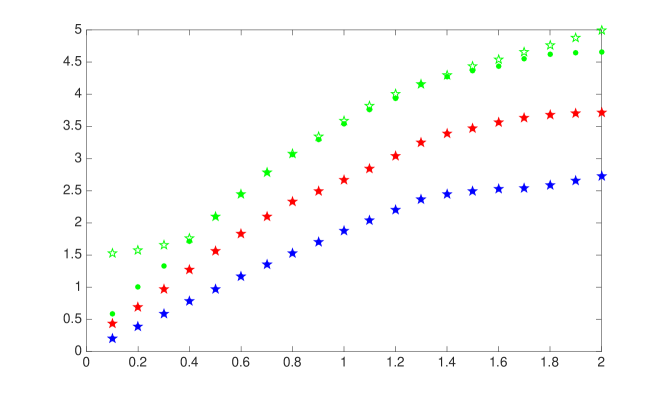
Figure 1: The SSP-TS coefficient ${\cal{C}}_{TS}$ (on y-axis) of fourth order SSP-TS M1 and M2 methods with $s={\color[rgb]{0,0,1}3},{\color[rgb]{1,0,0}4},{\color[rgb]{0,1,0}5}$ stages plotted against the value of $K$ (on x-axis). The open stars indicate methods of type (M1) while the filled circles are methods of type (M2). Filled stars are (M1) markers overlaid with (M2) markers indicating close if not equal SSP coefficients.

3.1 Fourth Order Methods

Using the optimization approach described above, we find fourth order methods with $s=3,4,5$ stages for a range of $K=0.1,...,2.0$. In Figure 1 we show the SSP coefficients of methods of SSP-TS methods of type (M1) and (M2) with $s=3,4,5$ (in blue, red, green) plotted against the value of $K$. The open stars indicate methods of type (M1) while the filled circles are methods of type (M2). Filled stars are (M1) markers overlaid with (M2) markers indicating close if not equal SSP coefficients.

Three Stage Methods: Three stage SSP-TS methods with fourth order accuracy exist, and all these have stage order two ($q=2$), so they are all of type (M2). Figure 1 shows the SSP coefficients of these methods in blue. The (M3) methods have an SSP coefficient

$${\cal{C}}_{TS}=\left\{\begin{array}[]{ll}\frac{2K}{K+1}&\mbox{for}\;\;\;K\leq 1\\ 1&\mbox{for}\;\;\;K\geq 1.\\ \end{array}\right.$$

For the case where $K\geq 1$ we obtain the following optimal (M3) scheme with a SSP coefficient ${\cal{C}}_{TS}=1$:

$$\begin{array}[]{l l}\vspace{.25 cm}y^{(1)}&=u^{n}\\ \vspace{.25 cm}y^{(2)}&=u^{n}+\Delta tF(y^{(1)})+\frac{1}{2}\Delta t^{2}\dot{F}(y^{(1)})\\ \vspace{.25 cm}y^{(3)}&=u^{n}+\frac{1}{27}\Delta t\left(14F(y^{(1)})+4F(y^{(2)})\right)+\frac{2}{27}\Delta t^{2}\dot{F}(y^{(1)})\\ \vspace{.25 cm}u^{n+1}&=u^{n}+\frac{1}{48}\Delta t\left(17F(y^{(1)})+4F(y^{(2)})+27F(y^{(3)})\right)+\frac{1}{24}\Delta t^{2}\dot{F}(y^{(1)}).\\ \end{array}$$

When $K\leq 1$ we have to modify the coefficients accordingly to obtain the maximal value of ${\cal{C}}_{TS}$ as defined above. Here we provide the non-zero coefficients for this family of M3(3,4,K) as a function of K:

$$\begin{array}[]{l l l}\vspace{.25 cm}a_{21}=\frac{K+1}{2}&b_{1}=\frac{3K^{5}-9K^{4}-22K^{3}+30K^{2}+21K+11}{3(K-3)^{2}(K+1)^{3}}&\hat{a}_{21}=\frac{(K+1)^{2}}{8}\\ \vspace{.25 cm}a_{31}=\frac{(K+1)(-K^{3}-2K^{2}+14K+3)}{2(K+2)^{3}}&b_{2}=\frac{2K}{3(K+1)^{3}}&\hat{a}_{31}=\frac{K(-K^{2}+2K+3)^{2}}{8(K+2)^{3}}\\ \vspace{.25 cm}a_{32}=\frac{(K+1)(K-3)^{2}}{2(K+2)^{3}}&b_{3}=\frac{2(K+2)^{3}}{3(K-3)^{2}(K+1)^{3}}&\hat{b}_{1}=-\frac{-3K^{3}+3K^{2}+K+1}{6(K-3)(K+1)^{2}}.\\ \end{array}$$

In Table 1 we compare the SSP coefficient of three stage fourth order SSP-TS methods of type (M2) and (M3) for a selection of values of $K$. Clearly, the (M3) methods have a much smaller SSP coefficient than the (M2) methods. However, a better measure of efficiency is the effective SSP coefficient computed by normalizing for the number of function evaluations required, which is $2s$ for the (M2) methods, and $s+1$ for the (M3) methods. If we consider the effective SSP coefficient, we find that while the (M2) methods are more efficient for the larger values of $K$, for smaller values of $K$ the (M3) methods are more efficient.

	K =	0.1	0.2	0.5	1.0	1.5	2.0
(M2)	${\cal{C}}_{TS}$ =	0.1995	0.3953	0.9757	1.8789	2.4954	2.7321
	${\cal{C}}_{\textup{eff}}$=	0.0333	0.0659	0.1626	0.3131	0.4159	0.4553
(M3)	${\cal{C}}_{TS}$ =	0.1818	0.3333	0.6667	1.0000	1.0000	1.0000
	${\cal{C}}_{\textup{eff}}$ =	0.0454	0.0833	0.1667	0.2500	0.2500	0.2500

Table 1: SSP-TS coefficients of three stage fourth order SSP-TS methods.

	K =	0.1	0.2	0.3	.5	1.0	1.5	1.6	1.8	2.0
(M1)	${\cal{C}}_{TS}$ =	0.4400	0.6921	0.9662	1.5617	2.6669	3.4735	3.5607	3.6759	3.7161
	${\cal{C}}_{\textup{eff}}$ =	0.0550	0.0865	0.1208	0.1952	0.3334	0.4342	0.4451	0.4595	0.4645
(M2)	${\cal{C}}_{TS}$ =	0.3523	0.6569	0.9662	1.5617	2.6669	3.4735	3.5301	3.5850	3.6282
	${\cal{C}}_{\textup{eff}}$ =	0.0440	0.0821	0.1208	0.1952	0.3334	0.4342	0.4413	0.4481	0.4535
(M3)	${\cal{C}}_{TS}$ =	0.3381	0.6102	0.8407	1.2174	1.8181	2.0596	2.0793	2.1030	2.1093
	${\cal{C}}_{\textup{eff}}$ =	0.0676	0.1220	0.1681	0.2435	0.3636	0.4119	0.4159	0.4206	0.4219

Table 2: SSP-TS coefficients of four stage fourth order SSP-TS methods.

	K	= 0.1	0.2	0.3	.5	.6	.7	1.0	1.5	2.0
(M1)	${\cal{C}}_{TS}$ =	1.5256	1.5768	1.6563	2.0934	2.4472	2.7819	3.5851	4.4371	4.9919
	${\cal{C}}_{\textup{eff}}$ =	0.1526	0.1577	0.1656	0.2093	0.2447	0.2782	0.3585	0.4437	0.4992
(M2)	${\cal{C}}_{TS}$ =	0.5876	1.0003	1.3319	2.0934	2.4472	2.7819	3.5381	4.3629	4.6614
	${\cal{C}}_{\textup{eff}}$ =	0.0588	0.1000	0.1332	0.2093	0.2447	0.2782	0.3538	0.4363	0.4661
(M3)	${\cal{C}}_{TS}$ =	0.5631	0.9296	1.2057	1.6551	1.8554	2.0300	2.4407	2.8748	2.9768
	${\cal{C}}_{\textup{eff}}$ =	0.0939	0.1549	0.2009	0.2758	0.3092	0.3383	0.4068	0.4791	0.4961

Table 3: SSP-TS coefficients of five stage fourth order methods.

Four Stage SSP-TS Methods: While four stage fourth order explicit SSP Runge-Kutta methods do not exist, four stage fourth order SSP-TS explicit two-derivative Runge-Kutta methods do. Four stage fourth order methods do not necessarily satisfy the stage order two ($q=2$) condition. These methods have a more nuanced behavior: for very small $K<0.2$, the optimized SSP methods have stage order $q=1$. For $0.2<K<1.6$ the optimized SSP methods have stage order $q=2$. Once $K$ becomes larger again, for $K\geq 1.6$, the optimized SSP methods are once again of stage order $q=1$. However, the difference in the SSP coefficients is very small (so small it does not show on the graph) so the (M2) methods can be used without significant loss of efficiency.

As seen in Table 2, the methods with the special structure (M3) have smaller SSP coefficients. But when we look at the effective SSP-TS coefficient we notice that, once again, for smaller $K$ they are more efficient. Table 2 shows that the (M3) methods are more efficient when $K\leq 1.5$, and remain competitive for larger values of $K$.

It is interesting to consider the limiting case, SSP-TS M2($4,4,\infty$), in which the Taylor series formula is unconditionally stable (i.e., $K=\infty$). This provides us with an upper bound of the SSP coefficient for this class of methods by ignoring any time step constraint coming from condition (14). A four stage fourth order method that is optimal for $K=\infty$ is:

$$\begin{array}[]{l l}\vspace{.25 cm}y^{(1)}&=u^{n}\\ \vspace{.25 cm}y^{(2)}&=u^{n}+\frac{1}{4}\Delta tF(y^{(1)})+\frac{1}{32}\Delta t^{2}\dot{F}(y^{(1)})\\ \vspace{.25 cm}y^{(3)}&=u^{n}+\frac{1}{4}\Delta t\left(F(y^{(1)})+F(y^{(2)})\right)+\frac{1}{32}\Delta t^{2}\left(\dot{F}(y^{(1)})+\dot{F}(y^{(2)})\right)\\ \vspace{.25 cm}y^{(4)}&=u^{n}+\frac{1}{4}\Delta t\left(F(y^{(1)})+F(y^{(2)})+F(y^{(3)})\right)+\frac{1}{32}\Delta t^{2}\left(\dot{F}(y^{(2)})+2\dot{F}(y^{(3)})\right)\\ \vspace{.25 cm}u^{n+1}&=u^{n}+\frac{1}{4}\Delta t\left(F(y^{(1)})+F(y^{(2)})+F(y^{(3)})+F(y^{(4)})\right)\\ &+\frac{1}{288}\Delta t^{2}\left(5\dot{F}(y^{(1)})+12\dot{F}(y^{(2)})+3\dot{F}(y^{(3)})+16\dot{F}(y^{(4)})\right).\\ \end{array}$$

This method has SSP coefficient ${\cal{C}}_{TS}=4$, with effective SSP coefficient ${\cal{C}}_{\textup{eff}}=\frac{1}{2}$. This method also has stage order $q=2$. This method is not intended to be useful in the SSP context but gives us an idea of the limiting behavior: i.e., what the best possible value of ${\cal{C}}_{TS}$ could be if the Taylor series condition had no constraint ($K=\infty)$. We observe in Table 2 that the SSP coefficient of the M2(4,4,K) method is within 10% of this limiting ${\cal{C}}_{TS}$ for values of $K=2$.

Five Stage Methods: The optimized five stage fourth order methods have stage order $q=2$ for the values of $0.5\leq K\leq 7$, and otherwise have stage order $q=1$. The SSP coefficients of these methods are shown in the green line in Figure 1, and the SSP and effective SSP coefficients for all three types of methods are compared in Table 3. We observe that these methods have higher effective SSP coefficients than the corresponding four stage methods.

3.2 Fifth Order SSP-TS Methods

While fifth order explicit SSP Runge-Kutta methods do not exist, the addition of a second derivative which satisfies the Taylor Series condition allows us to find explicit SSP-TS methods of fifth order. For fifth order, we have the result (in Section 2.2 above) that all methods must satisfy the stage order $q=2$ condition, so we consider only (M2) and (M3) methods. In Figure 3 we show the SSP-TS coefficients of M2(s,5,K) methods for $s=4,5,6$.

Four Stage Methods: Four stage fifth order methods exist, and their SSP-TS coefficients are shown in blue in Figure 3. We were unable to find M3(4,5,K) methods, possibly due to the paucity of available coefficients for this form.

Five Stage Methods: The SSP coefficient of the five stage M2 methods can be seen in red in Figure 3. We observe that the SSP coefficient of the M2(5,5,K) methods plateaus with respect to $K$. As shown in Table 4, methods with the form (M3) have a significantly smaller SSP coefficient than that of (M2). However, the effective SSP coefficient is more informative here, and we see that the (M3) methods are more efficient for small values of $K\leq 0.5$, but not for larger values.

Six Stage Methods: The SSP coefficient of the six stage M2 methods can be seen in green in Figure 3. In Table 4 we compare the SSP coefficients and effective SSP coefficients of (M2) and (M3) methods. As in the case above, the methods with the form (M3) have a significantly smaller SSP coefficient than that of (M2), and the SSP coefficient of the (M3) methods plateaus with respect to $K$. However, the effective SSP coefficient shows that the (M3) methods are more efficient for small values of $K\leq 0.7$, but not for larger values.

	K =	0.1	0.2	0.3	0.5	1.0	1.5	1.6	1.8	2.0
M2(5,5,K)	${\cal{C}}_{TS}$ =	0.3802	0.7448	1.0892	1.6877	2.9281	3.8102	3.8479	3.8879	3.8971
	${\cal{C}}_{\textup{eff}}$ =	0.0380	0.0745	0.1089	0.1688	0.2928	0.3810	0.3848	0.3888	0.3897
M3(5,5,K)	${\cal{C}}_{TS}$ =	0.3298	0.5977	0.8186	1.0625	1.0625	1.0625	1.0625	1.0625	1.0625
	${\cal{C}}_{\textup{eff}}$ =	0.0550	0.0996	0.1364	0.1771	0.1771	0.1771	0.1771	0.1771	0.1771
M2(6,5,K)	${\cal{C}}_{TS}$ =	0.5677	1.0230	1.4581	2.2102	3.8749	4.9201	5.0002	5.0903	5.1301
	${\cal{C}}_{\textup{eff}}$ =	0.0473	0.0852	0.1215	0.1842	0.3229	0.4100	0.4167	0.4242	0.4275
M3(6,5,K)	${\cal{C}}_{TS}$ =	0.5398	0.9370	1.2592	1.6914	1.8208	1.8208	1.8208	1.8208	1.8208
	${\cal{C}}_{\textup{eff}}$ =	0.0771	0.1339	0.1799	0.2416	0.2601	0.2601	0.2601	0.2601	0.2601

Table 4: SSP-TS coefficients and effective SSP-TS coefficients of fifth order methods.

	K =	0.1	0.2	0.3	0.5	1.0	1.5	2.0
M2(5,6,K)	${\cal{C}}_{TS}$	0.1441	0.2280	0.2780	0.3242	0.3500	0.3536	0.3555
	${\cal{C}}_{\textup{eff}}$	0.0144	0.0228	0.0278	0.0324	0.0350	0.0354	0.0355
M2(6,6,K)	${\cal{C}}_{TS}$	0.2944	0.5157	0.6725	0.9044	1.5225	2.0002	2.1966
	${\cal{C}}_{\textup{eff}}$	0.0245	0.0430	0.0560	0.0754	0.1269	0.1667	0.1831
M2(7,6,K)	${\cal{C}}_{TS}$	0.3981	0.7158	0.9734	1.4217	2.0376	2.5648	2.7794
	${\cal{C}}_{\textup{eff}}$	0.0284	0.0511	0.0695	0.1016	0.1455	0.1832	0.1985
M3(7,6,K)	${\cal{C}}_{TS}$	0.3547	0.6007	0.8059	0.8941	0.8947	0.8947	0.8947
	${\cal{C}}_{\textup{eff}}$	0.0443	0.0751	0.1007	0.1118	0.1118	0.1118	0.1118
M3(8,6,K)	${\cal{C}}_{TS}$	0.5495	0.9754	1.2882	1.6435	1.7369	1.7369	1.7369
	${\cal{C}}_{\textup{eff}}$	0.0611	0.1084	0.1431	0.1826	0.1930	0.1930	0.1930

Table 5: SSP-TS coefficients and effective SSP-TS coefficients of sixth orderSSP-TS methods.

3.3 Sixth Order SSP-TS Methods

As shown in Section 2.2, the highest order of accuracy this class of methods can obtain is $p=6$, and these methods must satisfy (28). We find sixth order methods with $s=5,6,7$ stages of type (M2). As to methods with the special structure M3, we are unable to find methods with $s\leq p$, but we find M3(7,6,K) methods and M3(8,6,K) methods. In the first six rows of Table 5 we compare the SSP-TS and effective SSP-TS coefficients of the (M2) methods with $s=5,6,7$ stages. In the last four rows of Table 5 we compare the SSP coefficients and effective SSP coefficients for sixth order methods with $s=7,8$ stages. Figure 3 shows the SSP-TS coefficients of the optimized (M3) methods for seven and eight stages, which clearly plateau with respect to $K$ (as can be seen in the tables as well). For the sixth order methods, it is clear that M3(8,6,K) methods are most efficient for all values of $K$.

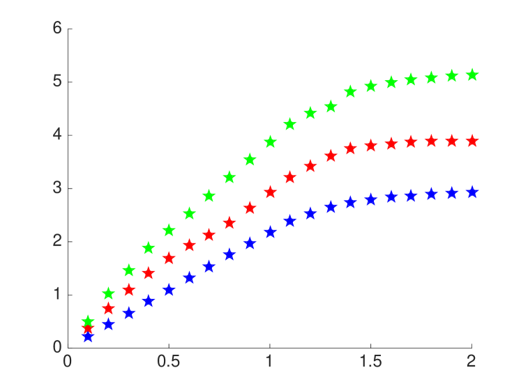
Figure 2: SSP-TS coefficients ${\cal{C}}_{TS}$ (on y-axis) for M2(4,5,K) and M2(5,5,K) and M2(6,5,K), where $K$ is on x-axis.

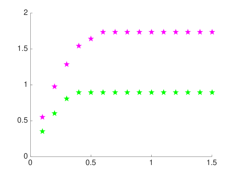
Figure 3: SSP-TS coefficients ${\cal{C}}_{TS}$ (on y-axis) for M3(7,6,K) and M3(8,6,K), where $K$ is on x-axis

3.4 Comparison with existing methods

First, we wish to compare the methods in this work to those in our prior work [5]. If a spatial discretization satisfies the forward Euler condition (12) and the second derivative condition (13) it will also satisfy the Taylor series condition (14), with

$$K=\tilde{K}\left(\sqrt{\tilde{K}^{2}+2}-\tilde{K}\right).$$

In this case, it is preferable to use the SSP-SD MDRK methods in [5]. However, in the case that the second derivative condition (13) is not satisfied for any value of $\tilde{K}>0$, or if the Taylor series condition is independently satisfied with a larger $K$ than would be established from the two conditions, i.e., $K>\tilde{K}\left(\sqrt{\tilde{K}^{2}+2}-\tilde{K}\right)$, then it may be preferable to use one of the SSP-TS methods derived in this work.

Next, we wish to compare the methods in this work to those in [33], which was the first paper to consider an SSP property based on the forward Euler and Taylor series base conditions. The approach used in our work is somewhat similar to that in [33] where the authors consider building time integration schemes which can be composed as convex combinations of forward Euler and Taylor series time steps, where they aim to find methods which are optimized for the largest SSP coefficients. However, there are several differences between our approach and the one of [33], which results in the fact that in this paper we are able to find more methods, of higher order, and with better SSP coefficients. In addition, in the present work we find and prove an order barrier for SSP-TS methods.

The first difference between our approach and the approach in [33] is that we allow computations of $\dot{F}$ of the intermediate values, rather than only $\dot{F}(u^{n})$. Another way of saying this is that we consider SSSP-TS methods that are not of type M3, while the methods considered in [33] are all of type M3. In some cases, when we restrict our search to M3 methods and $K=1$, we find methods with the same SSP coefficient as in [33]. For example, HBT34 matches our SSP-TS M3(3,4,1) method with an SSP coefficient of ${\cal{C}}_{TS}=1$, HBT44 matches our SSP-TS M3(4,4,1) method with ${\cal{C}}_{TS}=\frac{20}{11}$, HBT54 matches our SSP-TS M3(5,4,1) method with ${\cal{C}}_{TS}=2.441$, and HBT55 matches our SSP-TS M3(5,5,1) method with an SSP coefficient of ${\cal{C}}_{TS}=1.062$. While methods of type M3 have their advantages, they are sometimes sub-optimal in terms of efficiency, as we point out in the tables above.

The second difference between the SSP-TS methods in this paper and the methods in [33] is that in [33] only one method of order $p>4$ is reported, while we have many fifth and sixth order methods of various types and stages, optimized for a variety of $K$ values.

The most fundamental difference between our approach and the approach in [33] is that our methods are optimized for the relationship between the forward Euler restriction and the Taylor series restriction while the time step restriction in the methods of [33] is defined as the most restrictive of the forward Euler and Taylor series time step conditions. Respecting the minimum of the two cases will still satisfy the nonlinear stability property, but this approach does not allow for a balance between the restrictions considered, which can lead to severely more restrictive conditions. In our approach we use the relationship between the two time-step restrictions to select optimal methods. For this reason, the methods we find have larger allowable time-steps in many cases. To understand this a little better consider the case where the forward Euler condition is $\Delta t_{FE}\leq\Delta x$ and the Taylor series condition is $\Delta t_{TS}\leq\frac{1}{2}\Delta x$. In the approach used in [33], the base time step restriction is then $\Delta t_{max}=\max\{\Delta t_{FE},\Delta t_{TS}\}\leq\frac{1}{2}\Delta x$. The HBT23 method in [33] is a third order scheme with 2 stages which has a SSP coefficient of ${\cal{C}}_{TS}=1$, so the allowable time-step with this scheme will be the same $\Delta t\leq{\cal{C}}_{TS}\Delta t_{max}\leq\frac{1}{2}\Delta x$. On the other hand, using our optimal SSP-TS M2(2,3,.5) scheme, which has an SSP coefficient ${\cal{C}}_{TS}=.75$, the allowable time step is $\Delta t\leq{\cal{C}}_{TS}\Delta t_{FE}\leq\frac{3}{4}\Delta x$, a 50% increase. This is not only true when $K<1$: consider the case where $\Delta t_{FE}\leq\frac{1}{2}\Delta x$ and $\Delta t_{TS}\leq\Delta x$. Once again the HBT23 method in [33] will have a time step restriction of $\Delta t\leq{\cal{C}}_{TS}\Delta t_{max}\leq\frac{1}{2}\Delta x$, while our M2(2,3,2) method has an SSP coefficient ${\cal{C}}_{TS}=1.88$, so that the overall time step restriction would be $\Delta t\leq\frac{1.88}{2}\Delta x=.94\Delta x$, which is 88% larger. Even when the two base conditions are the same (i.e., $K=1$) and we have $\Delta t_{FE}\leq\Delta x$ and $\Delta t_{TS}\leq\Delta x$, the HBT23 method in [33] gives an allowable time-step of ${\cal{C}}_{TS}=1$ while our SSP-TS M2(2,3,1) has an SSP coefficient ${\cal{C}}_{TS}=1.5$, so that our method allows a time-step that is 50% larger. These simple cases demonstrate that our methods, which are optimized for the value of $K$, will usually allow a larger SSP coefficient that the methods obtained in [33].

4 Numerical Results

4.1 Overview of numerical tests

We wish to test our methods on what are now considered standard benchmark tests in the SSP community. In this subsection we preview our results, which we then present in more detail throughout the remainder of the section.

First, in the tests in Section 4.3 we focus on how the strong stability properties of these methods are observed in practice, by considering the total variation of the numerical solution. We focus on two scalar PDEs: the linear advection equation and Burgers’ equation, using simple first order spatial discretizations which are known to satisfy a total variation diminishing property over time for the forward Euler and Taylor series building blocks. We want to ensure that our numerical approximation to these solutions observe similar properties as long as the predicted SSP time step restriction, $\Delta t\leq{\cal{C}}_{TS}\Delta t_{FE}$, is respected. These scalar one-dimensional partial differential equations are chosen for their simplicity so we may understand the behavior of the numerical solution, but the discontinuous initial conditions may lead to instabilities if standard time discretization techniques are employed. Our tests show that the methods we design here preserve these properties as expected by the theory.

In Example 2, we extend the results from Example 1 to the case where we use the higher order weighted essentially non-oscillatory (WENO) method, which is not provably TVD but gives results that have very small increases in total variation. We demonstrate that our methods out-perform other methods, such as the SSP-SD MDRK methods in [5], and that non-SSP methods that are standard in the literature do not preserve the TVD property for any time-step.

In many of these examples we are concerned with the total variation diminishing property. To measure the sharpness of the SSP condition we compute the maximal observed rise in total variation over each step, defined by

$$\max_{0\leq n\leq N-1}\left(\|u^{n+1}\|_{TV}-\|u^{n}\|_{TV}\right),$$ (31)

as well as the maximal observed rise in total variation over each stage, defined by

$$\max_{1\leq j\leq s}\left(\|y^{(j+1)}\|_{TV}-\|y^{(j)}\|_{TV}\right),$$ (32)

where $y^{(s+1)}$ corresponds to $u^{n+1}$. The quantity of interest is the time-step $\Delta t_{obs}$, or the SSP coefficient ${\cal{C}}_{TS}^{obs}=\frac{\Delta t_{obs}}{\Delta t_{\textup{FE}}}$ at which this rise becomes significant, as defined by a maximal increase of $10^{-10}$.

It is important to notice that theSSP-TS methods we designed depend on the value of $K$ in (14). However, in practice we often do not know the exact value of $K$. In Example 3 we investigate what happens when we use spatial discretizations with a given value of $K$ with time discretization methods designed for an incorrect value of $K$. We conclude that although in some cases a smaller step-size is required, for methods of type M3 there is generally no adverse result from selecting the wrong value of $K$.

In Example 4 we investigate the increased flexibility in the choice of spatial discretization that results from relying on the (12) and (14) base conditions. The only constraint in the choice of differentiation operators $D_{x}$ and $\tilde{D}_{x}$ (described at the end of Section 1.2) is that the resulting building blocks must satisfy the monotonicity conditions (12) and (14) in the desired convex functional $\|\cdot\|$. As noted above, this constraint is less restrictive than requiring that (12) and (13) are satisfied: any spatial discretizations for which (12) and (13) are satisfied will also satisfy (14). However, there are some spatial discretizations that satisfy (12) and (14) that do not satisfy (13). In Example 4 we find that choosing spatial discretizations that satisfy (12) and (14) but not (13) allows for larger time-steps before the rise in total variation. And finally, in Example 5, we demonstrate the positivity preserving behavior of our methods when applied to a nonlinear system of equations.

4.2 On the numerical implementation of the second derivative.

In the following numerical test cases the spatial discretization is performed as follows: at each iteration we take the known value $u^{n}$ and compute the flux $f(u^{n})=-u^{n}$ in the linear case and $f(u^{n})=\frac{1}{2}\left(u^{n}\right)^{2}$ for Burgers’ equation. Now to compute the spatial derivative $f(u^{n})_{x}$ we use an operator $D_{x}$ and compute

$$u^{n}_{t}=-f(u^{n})_{x}\;\;\;\;\rightarrow\;\;\;\;u^{n}_{t}=D_{x}(-f(u^{n})).$$

In the numerical examples below the differential operator $D_{x}$ will represent, depending on the problem, a first order upwind finite difference scheme and the fifth order finite difference WENO method [21]. In our scalar test cases $f^{\prime}(u)$ does not change sign, so we avoid flux splitting.

Now we have the approximation to $U_{t}$ at time $t^{n}$, and wish to compute the approximation to $U_{tt}$. For the linear advection problem, this is very straightforward as $U_{tt}=U_{xx}$. To compute this, we take $u_{x}$ as computed before, and differentiate it again. For Burgers’ equation, we have $U_{tt}=\left(-UU_{t}\right)_{x}$. We take the approximation to $U_{t}$ that we obtained above,and we multiply it by $u^{n}$, then differentiate in space once again. In pseudocode, the calculation takes the form:

$$u^{n}_{tt}=(-f^{\prime}(u^{n})u^{n}_{t})_{x}\;\;\;\; \rightarrow\;\;\;\;u^{n}_{tt}=\tilde{D}_{x}(-f^{\prime}(u^{n})u^{n}_{t}).$$

Using these, we can now construct our two building blocks

$$\mbox{\bf Forward Euler}\;\;\;u^{n+1}=u^{n}+\Delta tu^{n}_{t},$$

$$\mbox{\bf Taylor series}\;\;\;u^{n+1}=u^{n}+\Delta tu^{n}_{t}+\frac{1}{2}\Delta t^{2}u^{n}_{tt}.$$

In choosing the spatial discretizarions $D_{x}$ and $\tilde{D}_{x}$ it is important that these building blocks satisfy (12) and (14) in the desired convex functional $\|\cdot\|$.

4.3 Example 1: TVD first order finite difference approximations

In this section we use first order spatial discretizations, that are provably total variation diminishing (TVD), coupled with a variety of time-stepping methods. We look at the maximal rise in total variation.

Example 1a: Linear advection. As a first test case, we consider a linear advection problem

$$U_{t}-U_{x}=0,$$ (33)

on a domain $x\in[-1,1]$, with step-function initial conditions

$$u_{0}(x)=\left\{\begin{array}[]{ll}1&\text{if}\ -\frac{1}{2}\leq x\leq\frac{1}{2},\\ 0&\text{otherwise},\end{array}\right.$$ (34)

and periodic boundary conditions. This simple example is chosen as our experience has shown [13] that this problem often demonstrates the sharpness of the SSP time-step.

Linear Advection
method	${\cal{C}}_{TS}^{pred}$	${\cal{C}}_{TS}^{obs}$	${\cal{C}}_{\textup{eff}}^{pred}$	${\cal{C}}_{\textup{eff}}^{obs}$
FE	1.0000	1.0000	1.00	1.00
TS	1.0000	1.0000	0.50	0.50
M2(3,4,1)	1.8788	1.8788	0.31	0.31
M3(3,4,1)	1.0000	1.0000	0.25	0.25
M2(4,4,1)	2.6668	2.6668	0.33	0.33
M3(4,4,1)	1.8181	1.8181	0.36	0.36
M2(5,4,1)	3.5381	3.6291	0.35	0.36
M3(5,4,1)	2.4406	2.4406	0.40	0.40
M2(4,5,1)	2.1864	2.2239	0.27	0.27
M2(5,5,1)	2.9280	3.1681	0.29	0.31
M3(5,5,1)	1.0625	1.5710	0.17	0.26
M2(6,5,1)	3.8749	3.8749	0.32	0.32
M3(6,5,1)	1.8207	1.9562	0.26	0.27
M2(5,6,1)	0.3500	1.9398	0.03	0.19
M2(6,6,1)	1.5225	2.3548	0.12	0.19
M2(7,6,1)	2.1150	2.3695	0.15	0.19
M3(7,6,1)	0.8946	1.3207	0.11	0.16
M3(8,6,1)	1.7369	1.9861	0.19	0.22

Burgers’
method	${\cal{C}}_{TS}^{pred}$	${\cal{C}}_{TS}^{obs}$	${\cal{C}}_{\textup{eff}}^{pred}$	${\cal{C}}_{\textup{eff}}^{obs}$
FE	1.0000	1.0000	1.00	1.00
TS	1.0000	1.0000	0.50	0.50
M2(3,4,1)	1.8788	1.8788	0.31	0.31
M3(3,4,1)	1.0000	1.0000	0.25	0.25
M2(4,4,1)	2.6668	2.6668	0.33	0.33
M3(4,4,1)	1.8181	1.8181	0.36	0.36
M2(5,4,1)	3.5381	3.6102	0.35	0.36
M3(5,4,1)	2.4406	2.4406	0.40	0.40
M2(4,5,1)	2.1864	2.2130	0.27	0.27
M2(5,5,1)	2.9280	3.1009	0.29	0.31
M3(5,5,1)	1.0625	1.5436	0.17	0.25
M2(6,5,1)	3.8749	3.8749	0.32	0.32
M3(6,5,1)	1.8207	2.0003	0.26	0.28
M2(5,6,1)	0.3500	1.9239	0.03	0.19
M2(6,6,1)	1.5225	2.2875	0.12	0.19
M2(7,6,1)	2.1150	2.3189	0.15	0.16
M3(7,6,1)	0.8946	1.2893	0.11	0.16
M3(8,6,1)	1.7369	1.9734	0.19	0.21

Table 6: Example 1: ${\cal{C}}_{TS}^{pred}$ and ${\cal{C}}_{TS}^{obs}$ for SSP-TS M2 and M3 methods.

For the spatial discretization we use a first order forward difference for the first and second derivative:

$$F(u^{n})_{j}:=\frac{u^{n}_{j+1}-u^{n}_{j}}{\Delta x}\approx U_{x}(x_{j}),\;\;\;\;\;\;\mbox{and}\;\;\;\;\;\;\tilde{F}(u^{n})_{j}\approx\tilde{F}(u^{n})_{j}:=\frac{u^{n}_{j+2}-2u^{n}_{j+1}+u^{n}_{j}}{\Delta x^{2}}\approx U_{xx}(x_{j}).$$

These spatial discretizations satisfy:

Forward Euler condition        $u^{n+1}_{j}=u^{n}_{j}+\frac{\Delta t}{\Delta x}\left(u^{n}_{j+1}-u^{n}_{j}\right)$ is TVD for $\Delta t\leq\Delta x$,
and

Taylor series condition        $u^{n+1}_{j}=u^{n}_{j}+\frac{\Delta t}{\Delta x}\left(u^{n}_{j+1}-u^{n}_{j}\right)+\frac{1}{2}\left(\frac{\Delta t}{\Delta x}\right)^{2}\left(u^{n}_{j+2}-2u^{n}_{j+1}+u^{n}_{j}\right)$ is TVD for $\Delta t\leq\Delta x$.

So that $\Delta t_{\textup{FE}}=\Delta x$ and in this case we have $K=1$ in (14). Note that the second derivative discretization used above does not satisfy the Second Derivative condition (13), so that most of the methods we devised in [5] do not guarantee strong stability preservation for this problem.

For all of our simulations for this example, we use a fixed grid of $M=601$ points, for a grid size $\Delta x=\frac{1}{600}$, and a time-step $\Delta t=\lambda\Delta x$ where we vary $\lambda$ from $\lambda=0.05$ until beyond the point where the TVD property is violated. We step each method forward by $N=50$ time-steps and compare the performance of the various time-stepping methods constructed earlier in this work, for $K=1$. We define the observed SSP coefficient ${\cal{C}}_{TS}^{obs}$ as the multiple of $\Delta t_{\textup{FE}}$ for which the maximal rise in total variation exceeds $10^{-10}$.

We verify that the observed values of $\Delta t_{\textup{FE}}$ and $K$ match the predicted values, and test this problem to see how well the observed SSP coefficient ${\cal{C}}_{TS}^{obs}$ matches the predicted SSP coefficient ${\cal{C}}_{TS}^{pred}$ for the fourth, fifth, and sixth order methods. The results are listed in the left-hand columns of Table 6.

Example 1b: Burgers’ equation We repeat the example above with all the same parameters but for the problem

$$U_{t}+\left(\frac{1}{2}U^{2}\right)_{x}=0$$ (35)

on $x\in(-1,1)$. Here we use the spatial derivatives:

$$F(u^{n})_{j}:=-\frac{f^{n}_{j}-f^{n}_{j-1}}{\Delta x}\approx-f(U)_{x}(x_{j}),$$

and

$$\tilde{F}(u^{n})_{j}\approx\tilde{F}(u^{n})_{j}:=-\frac{f^{\prime}(u^{n}_{j})F(u^{n})_{j}-f^{\prime}(u^{n}_{j-1})F(u^{n})_{j-1}}{\Delta x}\approx(f^{\prime}(U)f(U)_{x})_{x}(x_{j}).$$

Using Harten’s lemma we can easily show that these definitions of $F$ and $\tilde{F}$ cause the Taylor series condition to be satisfied for $\Delta t\leq\Delta x$. The results are quite similar to those of the linear advection equation in Example 1a, as can be seen in the right-hand columns of Table 6.

The results from these two studies show that the SSP-TS methods provide a reliable guarantee of the allowable time-step for which the method preserves the strong stability condition in the desired norm. For methods of order $p=4$, we observe that the SSP coefficient is sharp: the predicted and observed values of the SSP coefficient are identical for all the fourth order methods tested. For methods of higher order ($p=5,6$) the observed SSP coefficient is often significantly higher than the minimal value guaranteed by the theory.

4.4 Example 2: Weighted essentially non-oscillatory (WENO) approximations

In this section we re-consider the nonlinear Burgers’ equation (35)

$$U_{t}+\left(\frac{U^{2}}{2}\right)_{x}=0,$$

on $x\in(-1,1)$. We use the step function initial conditions (34), and periodic boundaries. We use $M=201$ points in the spatial domain, so that $\Delta x=\frac{1}{100}$, and we step forward for $N=50$ time-steps and measure the maximal rise in total variation for each case.

For the spatial discretization, we use the fifth order finite difference WENO method [21] in space, as this is a high order method that can handle shocks. We describe this method in Appendix C. Recall that the motivation for the development of SSP multistage multi-derivative time-stepping is for use in conjunction with high order methods for problems with shocks. Ideally, the specially designed spatial discretizations satisfy (12) and (14). Although the weighted essentially non-oscillatory (WENO) methods do not have a theoretical guarantee of this type, in practice we observe that these methods do control the rise in total variation, as long as the step-size is below a certain threshold.

Below, we refer to the WENO method on a flux with $f^{\prime}(u)\geq 0$ as WENO⁺ defined in (41) and to to the corresponding method on a flux with $f^{\prime}(u)\leq 0$ as WENO^- defined in (42). Because $f^{\prime}(u)$ is strictly non-negative in this example, we do not need to use flux splitting, and use $D=$WENO⁺. For the second derivative we have the freedom to use $\tilde{D}_{x}=$ WENO⁺ or $\tilde{D}_{x}=$ WENO^-. In this example, we use $\tilde{D}_{x}=D_{x}=$ WENO⁺. In Example 4 below we show that this is more efficient.

In Figure 4 on the left, we compare the performance of our SSP-TS M3(7,5,1) andSSP-TS M2(4,5,1) methods, which both have eight function evaluations per time-step, and our SSP-TS M3(5,5,1), which has six function evaluations per time-step, to the SSP-SD MDRK(3,5,2) in [5] and non-SSP RK(6,5) Dormand-Prince method [8], which also have six function evaluations per time-step. We note that we use the SSP-SD MDRK(3,5,2) (designed for $K=2$) because this method performs best compared to other explicit two-derivative multistage methods designed for different values of $K$. Clearly, the non-SSP method is not safe to use on this example. The M3 methods are most efficient, allowing the largest time-step per function evaluation before the total variation begins to rise.

This conclusion is also the case for the sixth order methods. In Figure 4 on the right, we compare our SSP-TS M3(9,6,1) and M2(5,6,1) methods, which both have ten function evaluations per time-step, and our M3(7,6,1), which has eight function evaluations per time-step, to the SSP-SD MDRK(4,6,1) and non-SSP RK(8,6) method given in Verner’s paper table [53], which also have eight function evaluations per time-step. Clearly, the non-SSP method is not safe to use on this example. The M3 methods are most efficient, allowing the largest time-step per function evaluation before the total variation begins to rise.

This example demonstrates the need for SSP methods: classical non-SSP methods do not control the rise in total variation. We also observe that the methods of type M3 are efficient, and may be the preferred choice of methods for use in practice.

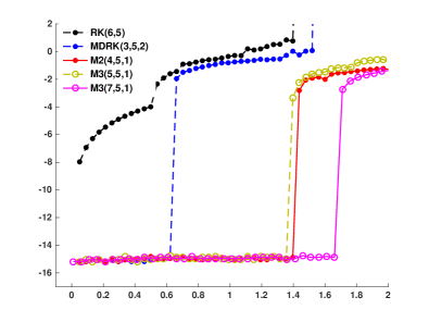
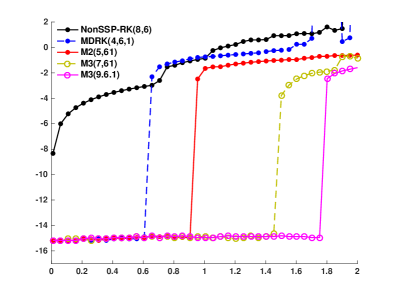
Figure 4: Example 2: Comparison of the maximal rise in total variation (on y-axis) as a function of $\lambda=\frac{\Delta t}{\Delta x}$ (on x-axis) for a selection of time-stepping methods for evolving Burgers’ equation with WENO spatial discretizations. Left: fifth order methods. Right: sixth order methods.

4.5 Example 3: Testing methods designed with various values of $K$

In general, the value of $K$ is not exactly known for a given problem, so we cannot choose a method that is optimized for the correct $K$. We wish to investigate how methods with different values of $K$ perform for a given problem. In this example, we re-consider the linear advection equation (33)

$$U_{t}=U_{x}$$

with step function initial conditions (34), and periodic boundary conditions on $x\in(-1,1)$. We use the fifth order WENO method with $M=201$ points in the spatial domain, so that $\Delta x=\frac{1}{100}$, and we step forward for $N=50$ time-steps and measure the maximal rise in total variation for each case. Using this example, we investigate how time-stepping methods optimized for different $K$ values perform on the linear advection with finite difference spatial approximation test case above, where it is known that $K=1$. We use a variety of fifth and sixth order methods, designed for $0.1\leq K\leq 2$ and give the value of $\lambda=\frac{\Delta t}{\Delta x}$ for which the maximal rise in total variation becomes large, when applied to the linear advection problem.

In Figure 5 (left) we give the observed value (solid lines) of $\lambda$ for a number of SSP-TS methods, M2(4,5,K), M2(5,5,K), M2(6,5,K), M3(5,5,K), and M3(6,5,K), and the corresponding predicted value (dotted lines) that a method designed for $K=1$ should give. In Figure 5 (right) we repeat this study with sixth order methods M2(5,6,K), M2(6,6,K), M3(7,6,K), and M3(8,6,K). We observe that while choosing the correct $K$ value can be beneficial, and is certainly important theoretically, in practice using methods designed for different $K$ values often makes little difference, particularly when the method is optimized for a value close to the correct $K$ value. For the sixth order methods in particular, the observed values of the SSP coefficient are all larger than the predicted SSP coefficient.

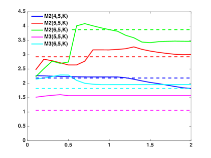
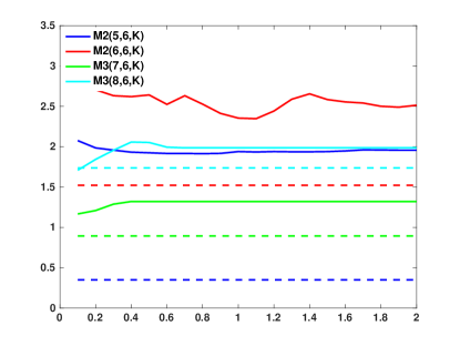
Figure 5: Example 3: The observed value of $\lambda=\frac{\Delta t}{\Delta x}$ such that the method is TVD (y-axis) when methods designed for different $K$ values (on x-axis) are applied to the problem with $K=1$. For each method, the observed value(solid line) is higher than the predicted value (dashed line).

4.6 Example 4: The benefit of different base conditions

In [5] we use the choice of $D_{x}=WENO^{+}$ defined in (41), followed by $\tilde{D}_{x}=WENO^{-}$ defined in (42), by analogy to the first order finite difference for the linear advection case $U_{t}=U_{x}$, where we use a differentiation operator $D_{x}^{+}$ followed by the downwind differentiation operator $D_{x}^{-}$ to produce a centered difference for the second derivative. In fact, this approach makes sense for these cases because it respects the properties of the flux for the second derivative and consequently satisfies the second derivative condition (13). However, if we simply wish the Taylor series formulation to satisfy a TVD-like condition, we are free to use the same operator ($WENO^{+}$ or $WENO^{-}$, as appropriate) twice, and indeed this gives a larger allowable $\Delta t$.

In Figure 6 we show how using the repeated upwind discretization $D=WENO^{-}$ and $\tilde{D}_{x}=WENO^{-}$ (solid lines) which satisfy the Taylor Series Condition (14) but not the second derivative condition (13) to approximate the higher order derivative allows for a larger time-step than the spatial discretizations (dashed lines) used in 9. We see that for the fifth order methods the rise in total variation always occurs for larger $\lambda$ for the solid lines ($\tilde{D}_{x}=D_{x}=WENO^{-}$) than for the dashed lines ($D_{x}=WENO^{-}$ and $\tilde{D}_{x}=WENO^{+}$), even for the method designed in [5] to be SSP for the second case but not the first case. For the sixth order methods the results are almost the same, though the SSP-SD MDRK(4,6,1) method that is SSP for base conditions of the type in [5] performs identically in both cases. These results demonstrate that requiring that the spatial discretizations only satisfy (12) and (14) (but not necessarily (13)) results in methods with larger allowable time-steps.

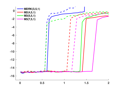
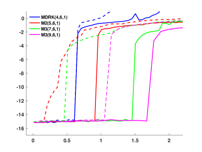
Figure 6: Example 4: The maximal rise in total variation (on y-axis) for values of $\lambda$ (on the x-axis). Simulations using the repeated upwind discretization $D_{x}=WENO^{-}$ and $\tilde{D}_{x}=WENO^{-}$ (solid lines) are more efficient than those using $D_{x}=WENO^{-}$ and $\tilde{D}_{x}=WENO^{+}$ (dashed lines). This demonstrates the enhanced allowable time-step afforded by the SSP-TS methods.

4.7 Example 5: Nonlinear Shallow Water Equations

As a final test case we consider the shallow water equations, where we are concerned with the preservation of positivity in the numerical solution. The shallow water equations [2] are a non-linear system of hyperbolic conservation laws defined by

$$\begin{pmatrix}h\\ hv\end{pmatrix}_{t}+\begin{pmatrix}hv\\ hv^{2}+\frac{1}{2}gh^{2}\end{pmatrix}_{x}=\begin{pmatrix}0\\ 0\end{pmatrix},$$

where $h(x,t)$ denotes the water height at location $x$ and time $t$, $v(x,t)$ the water velocity, $g$ is the gravitational constant, and $U=(h,hv)^{T}$ is the vector of unknown conserved variables. In our simulations, we set $g=1$. To discretize this problem, we use the standard Lax-Friedrichs splitting

$$\hat{f}_{j-1/2}:=\frac{1}{2}\left(f(u_{j})+f(u_{j-1})\right)-\frac{\alpha}{2}\left(u_{j}-u_{j-1}\right),\quad\alpha=\max_{j}\left\{|v_{j}\pm\sqrt{h_{j}}|\right\},$$

and define the (conservative) approximation to the first derivative as

$$f(U(x_{j}))_{x}\approx\frac{1}{\Delta x}\left(\hat{f}_{j+1/2}-\hat{f}_{j-1/2}\right).$$

We discretize the spatial grid $x\in(0,1)$ with $M=201$ points. To approximate the second derivative, we start with element-wise first derivative $u_{j,t}:=-\frac{1}{{\Delta x}}\left(\hat{f}_{j+1/2}-\hat{f}_{j-1/2}\right)$, and then approximate the second derivative (consistent with Eqn. (11)) as

$$u_{j,tt}:=-\frac{1}{2\Delta x}\left(f^{\prime}(u_{j+1})u_{j+1,t}-f^{\prime}(u_{j-1})u_{j-1,t}\right),$$

where $f^{\prime}(u_{j\pm 1})$ is the Jacobian of the flux function evaluated at $u_{j\pm 1}$. A simple first order spatial discretization is chosen here because it enables us to show that positivity is preserved for forward Euler and Taylor series for $\lambda^{+}_{FE}=\lambda^{+}_{TS}=\alpha\frac{\Delta t}{\Delta x}\leq 1$.

In problems such as the shallow water equations, the non-negativity of the numerical solution is important as a height of $h<0$ is not physically meaningful, and the system loses hyperbolicity when the height becomes negative. For a positivity preserving test case, we consider a Riemann problem with zero initial velocity, but with a wet and a dry state [2, 54]:

$$\left(h,v\right)^{T}=\begin{cases}(10,0)^{T}&x\leq 0.5,\\ (0,0)^{T}&x>0.5.\end{cases}$$

In our numerical simulations, we focus on the impact of the numerical scheme on the positivity of the solver for the the water height $h(x,t)$. This quantity is of interest from a numerical perspective because if the height $h(x,t)<0$ for any $x$ or $t$, the code will crash due to square-root of height.

Method	$\lambda^{pred}$	$\lambda^{obs}$	Method	$\lambda^{pred}$	$\lambda^{obs}$
Forward Euler	1.00000	1.01058	Taylor series	1.00000	1.02598
Dormand Prince	0.00000	0.00000	nonSSPRK(8,6)	0.00000	0.00000
SSP-SD MDRK(3,5,2)	–	1.03176	SSP-SD MDRK(4,6,1)	–	1.07803
SSP-TS M2(4,5,1)	2.18648	3.01005	SSP-TS M2(5,6,1)	0.35001	2.48411
SSP-TS M3(5,5,1)	1.06253	1.78593	SSP-TS M3(7,6,1)	0.89468	1.64084
SSP-TS M3(6,5,1)	1.82079	2.12579	SSP-TS M3(9,6,1)	2.59860	3.03387

Table 7: The predicted and observed values of $\lambda=\alpha\frac{\Delta t}{\Delta x}$ (where $\Delta x=\frac{1}{200}$) for which positivity of the height of the water is preserved in the shallow water equations in Example 5.

First, we investigate the behavior of the base methods in terms of the positivity preserving time step. In other words, we want to get a numerical value for $\Delta t_{\textup{FE}},K$. To do so, we numerically study the positivity behavior of the forward Euler and Taylor series approach. To do this, we evolve the solution forward for more time-steps with different values of $\lambda=\alpha\frac{\Delta t}{\Delta x}$ to identify the predicted positivity preserving value $\lambda^{pred}$. Using the approach, we see that as we increase the number of steps the predicted value of the positivity preserving value, $\lambda^{pred}_{FE}\rightarrow 1$ and $\lambda^{pred}_{TS}\rightarrow 1$, for both forward Euler and Taylor series. We are not able to numerically identify $\tilde{K}$ resulting from the second derivative condition, which cannot be evolved forward as it does not approximate the solution to the ODE at all.

In Table 7 we compare the positivity preserving time-step of a variety of numerical time integrators. We consider the fifth order SSP-TS methods M2(4,5,1), M3(5,5,1), and M3(6,5,1), and compare their performance to the SSP-SD MDRK(3,5,2) method in [5], and the non-SSP Dormand Prince method. We also consider the sixth order SSP-TS methods M2(5,6,1), M3(7,6,1), and M3(9,6,1), as well as the SSP-SD MDRK(4,6,1) from [5] and the non-SSPRK(8,6) method. Positivity of the water height is measure at each stage for a total of $N=60$ time-steps. We report the largest allowable value of $\lambda=\alpha\frac{\Delta t}{\Delta x}$ ($\alpha$ is the maximal wavespeed for the domain) for which the solution remains positive. For each method, the predicted values $\lambda^{pred}$ are obtained by multiplying the SSP coefficient ${\cal{C}}_{TS}$ of that method by $\lambda^{pred}_{FE}=\lambda^{pred}_{TS}=1$. For the SSP-SD MDRK methods we do not make a prediction as we are not able to identify the $\tilde{K}$ resulting from the second derivative condition.

In Table 7 we show that all of our SSP-TS methods preserve the positivity of the solution for values larger than those predicted by the theory $\lambda^{obs}>\lambda^{pred}$, and that even for the SSP MSRK methods there is a large region of values $\lambda^{obs}$ for which the solution remains positive. However, the non-SSP methods permit no positive time step that retains positivity of the solution, highlighting the importance of SSP methods.

5 Conclusions

In [5] we introduced a formulation and base conditions to extend the SSP framework to multistage multi-derivative time-stepping methods, and the resulting SSP-SD methods. While the choice of base conditions we used in [5] gives us more flexibility in finding SSP time stepping schemes, it limits the flexibility in the choice of the spatial discretization. In the current paper we introduce an alternative SSP formulation based on the conditions (12) and (14) and investigate the resulting explicit two-derivative multistage SSP-TS time integrators. These base conditions are relevant because some commonly used spatial discretizations may not satisfy the second derivative condition (13) which we required in [5], but do satisfy the Taylor series condition (14). This approach decreases the flexibility in our choice of time discretization because some time discretizations that can be decomposed into convex combinations of (12) and (13) cannot be decomposed into convex combinations of (12) and (14). However, it increases the flexibility in our choice of spatial discretizations, as we may now consider spatial methods that satisfy (12) and (14) but not (13). In the numerical tests we showed that this increased flexibility allowed for more efficient simulations in several cases.

In this paper, we proved that explicit SSP-TS methods have a maximum obtainable order of $p=6$. Next we formulated the proper optimization procedure to generate SSP-TS methods. Within this new class we were able to organize our schemes into three sub categories that reflect the different simplifications used in the optimization. We obtained methods up to and including order $p=6$ thus breaking the SSP order barrier for explicit SSP Runge-Kutta methods. Our numerical tests show that the SSP-TS explicit two-derivative methods perform as expected, preserving the strong stability properties satisfied by the base conditions (12) and (14) under the predicted time-step conditions. Our simulations demonstrate the sharpness of the SSP-TS condition in some cases, and the need for SSP-TS time-stepping methods. Furthermore the numerical results indicate that the added freedom in the choice of spatial discretization results in larger allowable time steps. The coefficients of the SSP-TS methods described in this work can be downloaded from [14].

Acknowledgements. The work of D.C. Seal was supported in part by the Naval Academy Research Council. The work of S. Gottlieb and Z.J. Grant was supported by the AFOSR grant #FA9550-15-1-0235.

A part of this research is sponsored by the Office of Advanced Scientific Computing Research; U.S. Department of Energy, and was performed at the Oak Ridge National Laboratory, which is managed by UT-Battelle, LLC under Contract No. De-AC05-00OR22725.

Notice: This manuscript has been authored by UT-Battelle, LLC, under contract DE-AC05-00OR22725 with the U.S. Department of Energy. The United States Government retains and the publisher, by accepting the article for publication, acknowledges that the United States Government retains a non-exclusive, paid-up, irrevocable, world-wide license to publish or reproduce the published form of this manuscript, or allow others to do so, for United States Government purposes.

Appendix A Order Conditions

Any method of the form (9) must satisfy the order conditions for all $p\leq P$ to be of order $P$.

$p=1$

$$b^{T}e=1\hskip 372.19005pt$$

$p=2$

$$b^{T}c+\hat{b}^{T}e=\frac{1}{2}\hskip 336.05505pt$$

$p=3$

$$b^{T}c^{2}+2\hat{b}^{T}c=\frac{1}{3}\hskip 180.67499pt$$

$$b^{T}Ac+b^{T}\hat{c}+\hat{b}^{T}c=\frac{1}{6}$$

$p=4$

$$b^{T}c^{3}+3\hat{b}^{T}c^{2}=\frac{1}{4}\hskip 325.215pt$$

$$b^{T}\left(c\odot Ac\right)+b^{T}\left(c\odot\hat{c}\right)+\hat{b}^{T}c^{2}+\hat{b}^{T}Ac+\hat{b}^{T}\hat{c}=\frac{1}{8}$$

$$b^{T}Ac^{2}+2b^{T}\hat{A}c+\hat{b}^{T}c^{2}=\frac{1}{12}$$

$$b^{T}A^{2}c+b^{T}A\hat{c}+b^{T}\hat{A}c+\hat{b}^{T}Ac+\hat{b}^{T}\hat{c}=\frac{1}{24}$$

$p=5$

$$b^{T}c^{4}+4\hat{b}^{T}c^{3}=\frac{1}{5}$$

$$b^{T}\left(c^{2}\odot Ac\right)+b^{T}\left(c^{2}\odot\hat{c}\right)+\hat{b}^{T}c^{3}+2\hat{b}^{T}\left(c\odot Ac\right)+2\hat{b}^{T}\left(c\odot\hat{c}\right)=\frac{1}{10}$$

$$b^{T}\left(c\odot Ac^{2}\right)+2b^{T}\left(c\odot\hat{A}c\right)+\hat{b}^{T}c^{3}+\hat{b}^{T}Ac^{2}+2\hat{b}^{T}\hat{A}c=\frac{1}{15}$$

$$b^{T}\left(c\odot A^{2}c\right)+b^{T}\left(c\odot A\hat{c}\right)+b^{T}\left(c\odot\hat{A}c\right)+\hat{b}^{T}\left(c\odot Ac\right)+\hat{b}^{T}\left(c\odot\hat{c}\right)+\hat{b}^{T}A^{2}c+\hat{b}^{T}A\hat{c}+\hat{b}^{T}\hat{A}c=\frac{1}{30}$$

$$b^{T}\left(Ac\odot Ac\right)+2b^{T}\left(\hat{c}\odot Ac\right)+b^{T}\hat{c}^{2}+2\hat{b}^{T}\left(c\odot Ac\right)+2\hat{b}^{T}\left(c\odot\hat{c}\right)=\frac{1}{20}$$

$$b^{T}Ac^{3}+3b^{T}\hat{A}c^{2}+\hat{b}^{T}c^{3}=\frac{1}{20}$$

$$b^{T}A\left(c\odot Ac\right)+b^{T}A\left(c\odot\hat{c}\right)+b^{T}\hat{A}c^{2}+b^{T}\hat{A}Ac+b^{T}\hat{A}\hat{c}+\hat{b}^{T}\left(c\odot Ac\right)+\hat{b}^{T}\left(c\odot\hat{c}\right)=\frac{1}{40}$$

$$b^{T}A^{2}c^{2}+2b^{T}A\hat{A}c+b^{T}\hat{A}c^{2}+\hat{b}^{T}Ac^{2}+2\hat{b}^{T}\hat{A}c=\frac{1}{60}$$

$$b^{T}A^{3}c+b^{T}A^{2}\hat{c}+b^{T}A\hat{A}c+b^{T}\hat{A}Ac+b^{T}\hat{A}\hat{c}+\hat{b}^{T}A^{2}c+\hat{b}^{T}A\hat{c}+\hat{b}^{T}\hat{A}c=\frac{1}{120}$$

$p=6$

$$b^{T}c^{5}+5\hat{b}^{T}c^{4}=\frac{1}{6}$$

$$b^{T}\left(c^{3}\odot Ac\right)+3\hat{b}^{T}\left(c^{2}\odot Ac\right)+\hat{b}^{T}c^{4}+b^{T}\left(c^{3}\odot\hat{c}\right)+3\hat{b}^{T}\left(c^{2}\odot\hat{c}\right)=\frac{1}{12}$$

$$b^{T}\left(c^{2}\odot Ac^{2}\right)+2\hat{b}^{T}\left(c\odot Ac^{2}\right)+2b^{T}\left(c^{2}\odot\hat{A}c\right)+\hat{b}^{T}c^{4}+4\hat{b}^{T}\left(c\odot\hat{A}c\right)=\frac{1}{18}$$

$$b^{T}\left(c\odot Ac^{3}\right)+3b^{T}\left(c\odot\hat{A}c^{2}\right)+\hat{b}^{T}Ac^{3}+3\hat{b}^{T}\hat{A}c^{2}+\hat{b}^{T}c^{4}=\frac{1}{24}$$

$$b^{T}Ac^{4}+4b^{T}\hat{A}c^{3}+\hat{b}^{T}c^{4}=\frac{1}{30}$$

$$b^{T}\left(c^{2}\odot A^{2}c\right)+2\hat{b}^{T}\left(c\odot A^{2}c\right)+b^{T}\left(c^{2}\odot A\hat{c}\right)+b^{T}\left(c^{2}\odot\hat{A}c\right)+\hat{b}^{T}\left(c^{2}\odot Ac\right)+2\hat{b}^{T}\left(c\odot A\hat{c}\right)$$

$$\;\;\;\;\;\;\;\;\;\;\;\;\;\;+2\hat{b}^{T}\left(c\odot\hat{A}c\right)+\hat{b}^{T}\left(c^{2}\odot\hat{c}\right)=\frac{1}{36}$$

$$b^{T}\left(c\odot A^{2}c^{2}\right)+\hat{b}^{T}A^{2}c^{2}+\hat{b}^{T}\left(c\odot Ac^{2}\right)+b^{T}\left(c\odot\hat{A}c^{2}\right)+2b^{T}\left(c\odot A\hat{A}c\right)+\hat{b}^{T}\hat{A}c^{2}+2\hat{b}^{T}A\hat{A}c$$

$$\;\;\;\;\;\;\;\;\;\;\;\;\;\;+2\hat{b}^{T}\left(c\odot\hat{A}c\right)=\frac{1}{72}$$

$$b^{T}A^{2}c^{3}+\hat{b}^{T}Ac^{3}+b^{T}\hat{A}c^{3}+3b^{T}A\hat{A}c^{2}+3\hat{b}^{T}\hat{A}c^{2}=\frac{1}{120}$$

$$b^{T}\left(c\odot Ac\odot Ac\right)+\hat{b}^{T}\left(Ac\odot Ac\right)+b^{T}\left(c\odot\hat{A}Ac\right)+b^{T}\left(c\odot A\left(c\odot\hat{c}\right)\right)+\hat{b}^{T}\left(c^{2}\odot Ac\right)+b^{T}\left(c\odot\hat{A}c^{2}\right)$$

$$\;\;\;\;\;\;\;\;\;\;\;\;\;\;+\hat{b}^{T}\hat{A}Ac+\hat{b}^{T}A\left(c\odot\hat{c}\right)+b^{T}\left(c\odot\hat{A}\hat{c}\right)+\hat{b}^{T}\hat{A}c^{2}+\hat{b}^{T}c^{2}\hat{c}+\hat{b}^{T}\hat{A}\hat{c}=\frac{1}{48}$$

$$b^{T}A\left(c^{2}\odot Ac\right)+b^{T}A\left(c^{2}\odot\hat{c}\right)+\hat{b}^{T}\left(c^{2}\odot Ac\right)+2b^{T}\left(\hat{A}c\odot Ac\right)+b^{T}\hat{A}c^{3}+2b^{T}\left(\hat{A}c\odot\hat{c}\right)$$

$$\;\;\;\;\;\;\;\;\;\;\;\;\;\;+\hat{b}^{T}\left(c^{2}\odot\hat{c}\right)=\frac{1}{60}$$

$$b^{T}\left(Ac\odot Ac^{2}\right)+\hat{b}^{T}\left(c\odot Ac^{2}\right)+b^{T}\hat{A}Ac^{2}+b^{T}\hat{A}c^{3}+2b^{T}\left(Ac\odot\hat{A}c\right)+2b^{T}\hat{A}^{2}c+2\hat{b}^{T}\left(c\odot\hat{A}c\right)=\frac{1}{90}$$

$$b^{T}\left(c\odot A^{3}c\right)+\hat{b}^{T}A^{3}c+\hat{b}^{T}\left(c\odot A^{2}c\right)+b^{T}\left(c\odot\hat{A}Ac\right)+b^{T}\left(c\odot A\hat{A}c\right)+b^{T}\left(c\odot A^{2}\hat{c}\right)+\hat{b}^{T}\hat{A}Ac$$

$$\;\;\;\;\;\;\;\;\;\;\;\;\;\;+\hat{b}^{T}A\hat{A}c+\hat{b}^{T}A^{2}\hat{c}+b^{T}\left(c\odot\hat{A}\hat{c}\right)+\hat{b}^{T}CA\hat{c}+\hat{b}^{T}C\hat{A}c+\hat{b}^{T}\hat{A}\hat{c}=\frac{1}{144}$$

$$b^{T}\left(Ac\odot A^{2}c\right)+b^{T}\left(Ac\odot A\hat{c}\right)+b^{T}\left(Ac\odot\hat{A}c\right)+b^{T}\left(\hat{A}c\odot Ac\right)+b^{T}\hat{A}A^{2}c+\hat{b}^{T}\left(c\odot A^{2}c\right)$$

$$\;\;\;\;\;\;\;\;\;\;\;\;\;\;+b^{T}\left(\hat{A}c\odot\hat{c}\right)+b^{T}\hat{A}A\hat{c}+\hat{b}^{T}\left(c\odot A\hat{c}\right)+b^{T}\hat{A}^{2}c+\hat{b}^{T}\left(c\odot\hat{A}c\right)=\frac{1}{180}$$

$$b^{T}(A^{2}\left(c\odot Ac\right)+b^{T}A^{2}\left(c\odot\hat{c}\right)+b^{T}A\hat{A}c^{2}+b^{T}A\hat{A}Ac+b^{T}\hat{A}\left(c\odot Ac\right)+\hat{b}^{T}A\left(c\odot Ac\right)+b^{T}A\hat{A}\hat{c}$$

$$\;\;\;\;\;\;\;\;\;\;\;\;\;\;+b^{T}\hat{A}\left(c\odot\hat{c}\right)+\hat{b}^{T}A\left(c\odot\hat{c}\right)+\hat{b}^{T}\hat{A}c^{2}+\hat{b}^{T}\hat{A}Ac+\hat{b}^{T}\hat{A}\hat{c}=\frac{1}{240}$$

$$b^{T}A^{3}c^{2}+\hat{b}^{T}A^{2}c^{2}+b^{T}\hat{A}Ac^{2}+b^{T}A\hat{A}c^{2}+2b^{T}A^{2}\hat{A}c+\hat{b}^{T}\hat{A}c^{2}+2\hat{b}^{T}A\hat{A}c+2b^{T}\hat{A}^{2}c=\frac{1}{360}$$

$$b^{T}\left(c\odot Ac\odot Ac\right)+\hat{b}^{T}\left(Ac\odot Ac\right)+2b^{T}\left(c\odot\hat{c}\odot Ac\right)+2\hat{b}^{T}\left(c^{2}\odot Ac\right)+2\hat{b}^{T}\left(\hat{c}\odot Ac\right)+2\hat{b}^{T}\left(c^{2}\odot\hat{c}\ \right)$$

$$\;\;\;\;\;\;\;\;\;\;\;\;\;\;+b^{T}\left(c\odot\hat{c}^{2}\right)+\hat{b}^{T}\hat{c}^{2}=\frac{1}{24}$$

$$b^{T}\left(Ac\odot A^{2}c\right)+b^{T}\left(\hat{c}\odot A^{2}c\right)+\hat{b}^{T}\left(c\odot A^{2}c\right)+\hat{b}^{T}\left(Ac\odot Ac\right)+b^{T}\left(Ac\odot\hat{A}c\right)+b^{T}\left(Ac\odot A\hat{c}\right)$$

$$\;\;\;\;\;\;\;\;\;\;\;\;\;\;+2\hat{b}^{T}\left(\hat{c}\odot Ac\right)+b^{T}\left(\hat{c}\odot\hat{A}c\right)+b^{T}\left(\hat{c}\odot A\hat{c}\right)+\hat{b}^{T}\left(c\odot\hat{A}c\right)+\hat{b}^{T}\left(c\odot A\hat{c}\right)+\hat{b}^{T}\hat{c}^{2}=\frac{1}{72}$$

$$b^{T}\left(Ac\odot Ac^{2}\right)+b^{T}\left(\hat{c}\odot Ac^{2}\right)+\hat{b}^{T}\left(c\odot Ac^{2}\right)+\hat{b}^{T}\left(Ac\odot c^{2}\right)+2b^{T}\left(Ac\odot\hat{A}c\right)+\hat{b}^{T}\left(\hat{c}\odot c^{2}\right)$$

$$\;\;\;\;\;\;\;\;\;\;\;\;\;\;+2b^{T}\left(\hat{c}\odot\hat{A}c\right)+2\hat{b}^{T}\left(c\odot\hat{A}c\right)=\frac{1}{36}$$

$$b^{T}A\left(Ac\odot Ac\right)+2b^{T}A\left(\hat{c}\odot Ac\right)+2b^{T}\hat{A}\left(c\odot Ac\right)+\hat{b}^{T}\left(Ac\odot Ac\right)+2\hat{b}^{T}\left(\hat{c}\odot Ac\right)+2b^{T}\hat{A}\left(c\odot\hat{c}\right)$$

$$\;\;\;\;\;\;\;\;\;\;\;\;\;\;+b^{T}A\hat{c}^{2}+\hat{b}^{T}\hat{c}^{2}=\frac{1}{120}$$

$$b^{T}A^{4}c+b^{T}A^{3}\hat{c}+b^{T}A^{2}\hat{A}c+b^{T}A\hat{A}Ac+b^{T}\hat{A}A^{2}c+\hat{b}^{T}A^{3}c+b^{T}A\hat{A}\hat{c}+b^{T}\hat{A}A\hat{c}+\hat{b}^{T}A^{2}\hat{c}$$

$$\;\;\;\;\;\;\;\;\;\;\;\;\;\;+b^{T}\hat{A}^{2}c+\hat{b}^{T}A\hat{A}c+\hat{b}^{T}\hat{A}Ac+\hat{b}^{T}\hat{A}\hat{c}=\frac{1}{720}$$

Appendix B Coefficients of selected methods

All the time-stepping methods in this work can be downloaded as Matlab files from [14]. In this appendix we present selected methods.

SSP-TS M2(4,5,1) : This method has ${\cal{C}}_{TS}=2.18648$

$$\begin{array}[]{lll}a_{21}=4.280141748183123e-01&\hat{a}_{21}=9.159806692270039e-02&b_{1}=3.456442194983256e-01\vspace{.1cm}\\ a_{31}=3.174364422211321e-01&\hat{a}_{31}=2.068159838961376e-02&b_{2}=1.551487425849178e-01\vspace{.1cm}\\ a_{32}=1.032647478325804e-01&\hat{a}_{32}=2.361437143530821e-02&b_{3}=3.458932447335502e-01\vspace{.1cm}\\ a_{41}=3.280547501426051e-01&\hat{a}_{41}=1.869435227642530e-02&b_{4}=1.533137931832064e-01\vspace{.1cm}\\ a_{42}=9.334228125655676e-02&\hat{a}_{42}=2.134532206271365e-02&\hat{b}_{1}=3.226836941745746e-02\vspace{.1cm}\\ a_{43}=4.134096583922347e-01&\hat{a}_{43}=9.453767556809974e-02&\hat{b}_{2}=1.785928934720153e-02\vspace{.1cm}\\ &&\hat{b}_{3}=7.490191551289183e-02\vspace{.1cm}\\ &&\hat{b}_{4}=3.505948481328697e-02\vspace{.1cm}\\ \end{array}$$

SSP-TS M3(8,6,1): This method has ${\cal{C}}_{TS}=1.7369$

$$\begin{array}[]{lll}a_{21}=3.498630949258150e-01&a_{65}=3.779563241192044e-01&\hat{a}_{21}=6.120209259553491e-02\vspace{.1cm}\\ a_{31}=2.253295269463227e-01&a_{71}=2.148681581922796e-01&\hat{a}_{31}=1.921063160949869e-02\vspace{.1cm}\\ a_{32}=1.807161013759724e-01&a_{72}=1.533420472452636e-01&\hat{a}_{41}=4.358605297856505e-03\vspace{.1cm}\\ a_{41}=2.071695605568409e-01&a_{73}=1.813808417863181e-02&\hat{a}_{51}=2.136333816692593e-03\vspace{.1cm}\\ a_{42}=4.100178308548576e-02&a_{74}=7.994387176143736e-02&\hat{a}_{61}=1.402456855983780e-03\vspace{.1cm}\\ a_{43}=1.306253212278126e-01&a_{75}=1.630752796649391e-01&\hat{a}_{71}=1.631142330728269e-02\vspace{.1cm}\\ a_{51}=1.667117585911237e-01&a_{76}=2.484093806816690e-01&\hat{a}_{81}=1.548804492637956e-02\vspace{.1cm}\\ a_{52}=2.009667996165993e-02&a_{81}=2.036762412289922e-01&b_{1}\;\;=1.927179349665056e-01\vspace{.1cm}\\ a_{53}=6.402490521280881e-02&a_{82}=1.456707401767411e-01&b_{2}\;\;=7.457643792836192e-02\vspace{.1cm}\\ a_{54}=2.821909187189924e-01&a_{83}=2.379744031395224e-02&b_{3}\;\;=1.097549250079706e-01\vspace{.1cm}\\ a_{61}=1.493141923275556e-01&a_{84}=1.048777345557326e-01&b_{4}\;\;=1.166274027628658e-01\vspace{.1cm}\\ a_{62}=1.319303489675465e-02&a_{85}=2.139668745571685e-01&b_{5}\;\;=1.862061970475841e-01\vspace{.1cm}\\ a_{63}=4.203095914776495e-02&a_{86}=6.560681670556633e-02&b_{6}\;\;=1.088089628270683e-01\vspace{.1cm}\\ a_{64}=1.852522020371737e-01&a_{87}=1.520556075200664e-01&b_{7}\;\;=4.414821350738243e-02\vspace{.1cm}\\ &&b_{8}\;\;=1.671599259522612e-01\vspace{.1cm}\\ &&\hat{b}_{1}\;\;=1.156518516980132e-02\vspace{.1cm}\\ \end{array}$$

Appendix C Fifth order WENO method of Jiang and Shu

To solve the PDE

$$u_{t}+f(u)_{x}=0$$

we approximate the spatial derivative to obtain $F(u)\approx-f(u)_{x}$, and then use a time-stepping method to solve the resulting system of ODEs. In this section we describe the fifth order WENO scheme presented in [21].

First, we split the flux into the positive and negative parts

$$f(u)=f^{+}(u)+f^{-}(u).$$

This can be accomplished in a variety of ways, e.g. the Lax-Friedrichs flux splitting

$$f^{+}(u)=\frac{1}{2}\left(f(u)+mu\right)\;\;\;\;f^{-}(u)=\frac{1}{2}\left(f(u)-mu\right),$$

where $m=\max|f^{\prime}(u)|$. In this way we ensure that $\frac{df^{+}}{du}\geq 0$ and $\frac{df^{-}}{du}\leq 0$.

To calculate the numerical fluxes $\hat{f}^{+}_{j+\frac{1}{2}}$ and $\hat{f}^{-}_{j+\frac{1}{2}}$, we begin by calculating the smoothness measurements to determine if a shock lies within the stencil. For our fifth order scheme, these are:

$$IS_{0}^{+} = \frac{13}{12}\left(f^{+}_{j-2}-2f^{+}_{j-1}+f^{+}_{j}\right)^{2}+\frac{1}{4}\left(f^{+}_{j-2}-4f^{+}_{j-1}+3f^{+}_{j}\right)^{2}$$

$$IS_{1}^{+} = \frac{13}{12}\left(f^{+}_{j-1}-2f^{+}_{j}+f^{+}_{j+1}\right)^{2}+\frac{1}{4}\left(f^{+}_{j-1}-f^{+}_{j+1}\right)^{2}$$

$$IS_{2}^{+} = \frac{13}{12}\left(f^{+}_{j}-2f^{+}_{j+1}+f^{+}_{j+2}\right)^{2}+\frac{1}{4}\left(3f^{+}_{j}-4f^{+}_{j+1}+f^{+}_{j+2}\right)^{2}$$

and

$$IS_{0}^{-} = \frac{13}{12}\left(f^{-}_{j+1}-2f^{-}_{j+2}+f^{-}_{j+3}\right)^{2}+\frac{1}{4}\left(3f^{-}_{j+1}-4f^{-}_{j+2}+f^{-}_{j+3}\right)^{2}$$

$$IS_{1}^{-} = \frac{13}{12}\left(f^{-}_{j}-2f^{-}_{j+1}+f^{-}_{j+2}\right)^{2}+\frac{1}{4}\left(f^{-}_{j}-f^{-}_{j+2}\right)^{2}$$

$$IS_{2}^{-} = \frac{13}{12}\left(f^{-}_{j-1}-2f^{-}_{j}+f^{-}_{j+1}\right)^{2}+\frac{1}{4}\left(f^{-}_{j-1}-4f^{-}_{j}+3f^{-}_{j+1}\right)^{2}\;.$$

Next, we use the smoothness measurements to calculate the stencil weights

$$\alpha^{\pm}_{0}=\frac{1}{10}\left(\frac{1}{\epsilon+IS_{0}^{\pm}}\right)^{2}\;\;\;\;\;\alpha^{\pm}_{1}=\frac{6}{10}\left(\frac{1}{\epsilon+IS_{1}^{\pm}}\right)^{2}\;\;\;\;\;\alpha^{\pm}_{2}=\frac{3}{10}\left(\frac{1}{\epsilon+IS_{2}^{\pm}}\right)^{2}$$

and

$$\omega^{\pm}_{0}=\frac{\alpha^{\pm}_{0}}{\alpha^{\pm}_{0}+\alpha^{\pm}_{1}+\alpha^{\pm}_{2}}\;\;\;\;\;\omega^{\pm}_{1}=\frac{\alpha^{\pm}_{1}}{\alpha^{\pm}_{0}+\alpha^{\pm}_{1}+\alpha^{\pm}_{2}}\;\;\;\;\;\omega^{\pm}_{2}=\frac{\alpha^{\pm}_{2}}{\alpha^{\pm}_{0}+\alpha^{\pm}_{1}+\alpha^{\pm}_{2}}.$$

Finally, the numerical fluxes are

$$\hat{f}^{+}_{j+\frac{1}{2}} = \omega^{+}_{0}\left(\frac{2}{6}f^{+}_{j-2}-\frac{7}{6}f^{+}_{j-1}+\frac{11}{6}f^{+}_{j}\right)+\omega^{+}_{1}\left(-\frac{1}{6}f^{+}_{j-1}+\frac{5}{6}f^{+}_{j}+\frac{2}{6}f^{+}_{j+1}\right)$$

$$+ \omega^{+}_{2}\left(\frac{2}{6}f^{+}_{j}+\frac{5}{6}f^{+}_{j+1}-\frac{1}{6}f^{+}_{j+2}\right)$$

and

$$\hat{f}^{-}_{j+\frac{1}{2}} = \omega^{-}_{2}\left(-\frac{1}{6}f^{-}_{j-1}+\frac{5}{6}f^{-}_{j}+\frac{2}{6}f^{-}_{j+1}\right)+\omega^{-}_{1}\left(\frac{2}{6}f^{-}_{j}+\frac{5}{6}f^{-}_{j+1}-\frac{1}{6}f^{-}_{j+2}\right)$$

$$+ \omega^{-}_{0}\left(\frac{11}{6}f^{-}_{j+1}-\frac{7}{6}f^{-}_{j+2}+\frac{2}{6}f^{-}_{j+3}\right).$$

Finally, we compute

$$WENO^{+}f^{+}(u) = -\frac{1}{\Delta x}\left(\hat{f}^{+}_{j+\frac{1}{2}}-\hat{f}^{+}_{j-\frac{1}{2}}\right)$$ (41)

$$WENO^{-}f^{-}(u) = -\frac{1}{\Delta x}\left(\hat{f}^{-}_{j+\frac{1}{2}}-\hat{f}^{-}_{j-\frac{1}{2}}\right)$$ (42)

and put it all together

$$F(u)=WENO^{+}f^{+}(u)+WENO^{-}f^{-}(u)\approx-f(u)_{x}.$$

References

- [1] C. Bresten, S. Gottlieb, Z. Grant, D. Higgs, D. I. Ketcheson, and A. Németh, Strong stability preserving multistep Runge-Kutta methods, Mathematics of Computation, 86 (2017), pp. 747–769.
- [2] S. Bunya, E. J. Kubatko, J. J. Westerink, and C. Dawson, A wetting and drying treatment for the Runge-Kutta discontinuous Galerkin solution to the shallow water equations, Comput. Methods Appl. Mech. Engrg., 198 (2009), pp. 1548–1562.
- [3] R. P. K. Chan and A. Y. J. Tsai, On explicit two-derivative Runge-Kutta methods, Numerical Algorithms, 53 (2010), pp. 171–194.
- [4] J. B. Cheng, E. F. Toro, S. Jiang, and W. Tang, A sub-cell WENO reconstruction method for spatial derivatives in the ADER scheme, Journal of Computational Physics 251 (2013), pp. 53 - 80.
- [5] A. Christlieb, S. Gottlieb, Z. Grant, and D. C. Seal, Explicit strong stability preserving multistage two-derivative time-stepping schemes, Journal of Scientific Computing, 68 (2016), pp. 914–942.
- [6] B. Cockburn and C.-W. Shu, TVB Runge-Kutta local projection discontinuous Galerkin finite element method for conservation laws II: general framework, Mathematics of Computation 52 (1989), pp. 411–435.
- [7] V. Daru and C. Tenaud, High order one-step monotonicity-preserving schemes for unsteady compressible flow calculations, Journal of Computational Physics 193 (2004), pp. 563–594.
- [8] J. R. Dormand and P. J. Prince, A family of embedded Runge-Kutta formulae, Journal of Computational and Applied Mathematics, 6 (1980), pp. 19–26.
- [9] Z. Du and J. Li, A Hermite WENO reconstruction for fourth order temporal accurate schemes based on the GRP solver for hyperbolic conservation laws, Journal of Computational Physics 355 (2018), pp. 385–396
- [10] M. Dumbser, O. Zanotti, A. Hidalgo, and D. S. Balsara, ADER-WENO finite volume schemes with space-time adaptive mesh refinement, Journal of Computational Physics 248 (2013), pp. 257 - 286.
- [11] L. Ferracina and M. N. Spijker, Stepsize restrictions for the total-variation-diminishing property in general Runge–Kutta methods, SIAM Journal of Numerical Analysis, 42 (2004), pp. 1073–1093.
- [12] , An extension and analysis of the Shu–Osher representation of Runge–Kutta methods, Mathematics of Computation, 249 (2005), pp. 201–219.
- [13] S. Gottlieb, D. I. Ketcheson, and C.-W. Shu, Strong Stability Preserving Runge–Kutta and Multistep Time Discretizations, World Scientific Press, 2011.
- [14] S. Gottlieb, Z. J. Grant, D. C. Seal, Explicit SSP multistage two-derivative methods with Taylor series base conditions. https://github.com/SSPmethods/SSPTSmethods.
- [15] Z. J. Grant, Explicit SSP multistage two-derivative SSP optimization code. https://github.com/SSPmethods/SSPMultiStageTwoDerivativeMethods, February 2015.
- [16] A. Harten, High resolution schemes for hyperbolic conservation laws, Journal of Computational Physics 49 (1983), pp. 357–393.
- [17] I. Higueras, On strong stability preserving time discretization methods, Journal of Scientific Computing, 21 (2004), pp. 193–223.
- [18] , Representations of Runge–Kutta methods and strong stability preserving methods, SIAM Journal On Numerical Analysis, 43 (2005), pp. 924–948.
- [19] I. Higueras, Characterizing Strong Stability Preserving Additive Runge-Kutta Methods, Journal of Scientific Computing, 39(1) (2009), pp. 115–128.
- [20] R. Jeltsch, Reducibility and contractivity of Runge–Kutta methods revisited, BIT Numerical Mathematics, 46(3) (2006), pp. 567–587.
- [21] G.-S. Jiang and C.-W. Shu, Efficient implementation of weighted ENO schemes, J. Comput. Phys., 126 (1996), pp. 202–228.
- [22] K. Kastlunger and G. Wanner, On Turan type implicit Runge-Kutta methods, Computing (Arch. Elektron. Rechnen), 9 (1972), pp. 317–325.
- [23] K. H. Kastlunger and G. Wanner, Runge Kutta processes with multiple nodes, Computing (Arch. Elektron. Rechnen), 9 (1972), pp. 9–24.
- [24] D. I. Ketcheson, Highly efficient strong stability preserving Runge–Kutta methods with low-storage implementations, SIAM Journal on Scientific Computing, 30 (2008), pp. 2113–2136.
- [25] D. I. Ketcheson, S. Gottlieb, and C. B. Macdonald, Strong stability preserving two-step Runge-Kutta methods, SIAM Journal on Numerical Analysis, (2012), pp. 2618–2639.
- [26] D. I. Ketcheson, C. B. Macdonald, and S. Gottlieb, Optimal implicit strong stability preserving Runge–Kutta methods, Applied Numerical Mathematics, 52 (2009), p. 373.
- [27] D. I. Ketcheson, M. Parsani, and A. J. Ahmadia, RK-Opt: software for the design of Runge–Kutta methods, version 0.2. https://github.com/ketch/RK-opt.
- [28] J. F. B. M. Kraaijevanger, Contractivity of Runge–Kutta methods, BIT, 31 (1991), pp. 482–528.
- [29] A. Kurganov and E. Tadmor, New high-resolution schemes for nonlinear conservation laws and convection-diffusion equations, Journal of Computational Physics 160 (2000), pp. 241–282.
- [30] J. Li and Z. Du, A two-stage fourth order time-accurate discretization for Lax-Wendroff type flow solvers I. hyperbolic conservation laws, SIAM J. Sci. Computing, 38 (2016) pp. 3046–3069.
- [31] X.-D. Liu, S. Osher and T. Chan, Weighted essentially non-oscillatory schemes, Journal of Computational Physics 115 (1994), pp. 200–212.
- [32] T. Mitsui, Runge-Kutta type integration formulas including the evaluation of the second derivative. i., Publications of the Research Institute for Mathematical Sciences, 18 (1982), pp. 325–364.
- [33] T. Nguyen-Ba, H. Nguyen-Thu, T. Giordano, and R. Vaillancourt, One-step strong-stability-preserving Hermite-Birkhoff-Taylor methods, Scientific Journal of Riga Technical University, 45 (2010), pp. 95–104.
- [34] N. Obreschkoff, Neue quadraturformeln, Abh. Preuss. Akad. Wiss. Math.-Nat. Kl., 4 (1940).
- [35] H. Ono and T. Yoshida, Two-stage explicit Runge-Kutta type methods using derivatives., Japan Journal of Industrial and Applied Mathematics, 21 (2004), pp. 361–374.
- [36] S. Osher and S. Chakravarthy, High resolution schemes and the entropy condition, SIAM Journal on Numerical Analysis 21(1984), pp. 955–984.
- [37] L. Pan, K. Xu, Q. Li, and J. Li, An efficient and accurate two-stage fourth-order gas-kinetic scheme for the Euler and Navier–Stokes equations, Journal of Computational Physics 326 (2016), pp. 197–221.
- [38] J. Qiu, M. Dumbser, and C.-W. Shu, The discontinuous Galerkin method with Lax–Wendroff type time discretizations, Computer Methods in Applied Mechanics and Engineering 194 (2005), pp. 4528–4543.
- [39] S. J. Ruuth and R. J. Spiteri, Two barriers on strong-stability-preserving time discretization methods, Journal of Scientific Computing, 17 (2002), pp. 211–220.
- [40] D. C. Seal, Y. Guclu, and A. J. Christlieb, High-order multiderivative time integrators for hyperbolic conservation laws, Journal of Scientific Computing, 60 (2014), pp. 101–140.
- [41] H. Shintani, On one-step methods utilizing the second derivative, Hiroshima Mathematical Journal, 1 (1971), pp. 349–372.
- [42] , On explicit one-step methods utilizing the second derivative, Hiroshima Mathematical Journali, 2 (1972), pp. 353–368.
- [43] C.-W. Shu, Total-variation diminishing time discretizations, SIAM Journal on Scientific and Statistical Computing, 9 (1988), pp. 1073–1084.
- [44] C.-W. Shu and S. Osher, Efficient implementation of essentially non-oscillatory shock-capturing schemes, Journal of Computational Physics, 77 (1988), pp. 439–471.
- [45] R. J. Spiteri and S. J. Ruuth, A new class of optimal high-order strong-stability-preserving time discretization methods, SIAM J. Numer. Anal., 40 (2002), pp. 469–491.
- [46] D. D. Stancu and A. H. Stroud, Quadrature formulas with simple Gaussian nodes and multiple fixed nodes, Mathematics of Computation, 17 (1963), pp. 384–394.
- [47] P.K. Sweby, High resolution schemes using flux limiters for hyperbolic conservation laws, SIAM Journal on Numerical Analysis 21 (1984), pp. 995–1011.
- [48] E. Tadmor, Approximate solutions of nonlinear conservation laws in Advanced Numerical Approximation of Nonlinear Hyperbolic Equations, Lectures Notes from CIME Course Cetraro, Italy, 1997, Number 1697 in Lecture Notes in Mathematics. Springer-Verlag, 1998.
- [49] E. Toro and V.A. Titarev, Solution of the generalized Riemann problem for advection–reaction equations, Proceedings of the Royal Society of London A: Mathematical, Physical and Engineering Sciences 458 (2002), pp. 271–281.
- [50] E.F. Toro and V.A. Titarev, Derivative Riemann solvers for systems of conservation laws and ADER methods, Journal of Computational Physics 212 (2006), pp. 150–165.
- [51] A. Y. J. Tsai, R. P. K. Chan, and S. Wang, Two-derivative Runge–Kutta methods for PDEs using a novel discretization approach, Numerical Algorithms, 65 (2014), pp. 687–703.
- [52] P. Turán, On the theory of the mechanical quadrature, Acta Universitatis Szegediensis. Acta Scientiarum Mathematicarum, 12 (1950), pp. 30–37.
- [53] J. Verner, Explicit runge kutta methods with estimates of the local truncation error, SIAM Journal on Numerical Analysis, 15 (2014), pp. 772–790.
- [54] Y. Xing, X. Zhang, and C.-W. Shu, Positivity-preserving high order well-balanced discontinuous Galerkin methods for the shallow water equations, Advances in Water Resources, 33 (2010), pp. 1476 – 1493.
- [55] X. Zhang and .C.-W. Shu, On Maximum-principle-satisfying High Order Schemes for Scalar Conservation Laws, Journal of Computational Physics 229 (2010), pp. 3091–3120.