BCOR5mm DIVclassic headincludefalse footincludefalse pagesizeauto headingssmall numbersendperiod 1pt 1pt Definition]Problem Definition]Assumption Definition]Theorem Definition]Proposition Definition]Lemma Definition]Corollary Definition]Algorithm  
Non-convex regularization of bilinear and quadratic inverse problems by tensorial lifting
Robert Beinert¹ and Kristian Bredies^1
1 Institut für Mathematik und Wissenschaftliches Rechnen Karl-Franzens-Universität Graz Heinrichstraße 36 8010 Graz, Austria
Correspondence
R. Beinert:
K. Bredies:
 
             Abstract.  Considering the question: how non-linear may a non-linear operator be in order to extend the linear regularization theory, we introduce the class of dilinear mappings, which covers linear, bilinear, and quadratic operators between Banach spaces. The corresponding dilinear inverse problems cover blind deconvolution, deautoconvolution, parallel imaging in MRI, and the phase retrieval problem. Based on the universal property of the tensor product, the central idea is here to lift the non-linear mappings to linear representatives on a suitable topological tensor space. At the same time, we extend the class of usually convex regularization functionals to the class of diconvex functionals, which are likewise defined by a tensorial lifting. Generalizing the concepts of subgradients and Bregman distances from convex analysis to the new framework, we analyse the novel class of dilinear inverse problems and establish convergence rates under similar conditions than in the linear setting. Considering the deautoconvolution problem as specific application, we derive satisfiable source conditions and validate the theoretical convergence rates numerically.
             Keywords.  ill-posed inverse problems, bilinear and quadratic equations, non-convex Tikhonov regularization, convergence rates, deautoconvolution
             AMS subject classification.  45Q05, 46A32, 47J06, 65J15
 

1 Introduction

Nowadays the theory of inverse problems has become one of the central mathematical approaches to solve recovery problems in medicine, engineering, and life sciences. Some of the main applications are computed tomography (CT), magnetic resonance imaging (MRI), and deconvolution problems in microscopy, see for instance [BB98, MS12, Ram05, SW13, Uhl03, Uhl13] being recent monographs as well as many other publications.

The beginnings of the modern regularization theory for ill-posed problems are tracing back to the pioneering works of A. N. Tikhonov [Tik63a, Tik63b]. Between then and now, the theory has been heavily extended and covers linear and non-linear formulations in the Hilbert space as well as in the Banach space setting. In order to name at least a few of the numerous monographs, we refer to [BG94, EHN96, Hof86, Lou89, LP13, Mor84, SKHK12, TA77, TLY98]. Due to the enormous relevance of the research topic, the published literature embraces many further monographs as well as a vast number of research articles.

Especially for linear problem formulations, the analytical framework is highly developed and allows the general treatment of inverse problems with continuous operators, see for instance [EHN96, MS12, SKHK12] and references therein. In addition to the sophisticated analysis, efficient numerical implementations of the solution schemes are available for practitioners [EHN96, Sch11]. The interaction between analysis and numerics are one reason for the great, interdisciplinary success of the linear regularization theory for ill-posed inverse problems.

If the linear operator in the problem formulation is replaced by a non-linear operator, the situation changes dramatically. Depending on the operator, there are several regularization approaches with different benefits and drawbacks [EHN96, Gra11, HKPS07, SGG⁺09]. One standard approach to regularize non-linear operators is to introduce suitable non-linearity conditions and to restrict the set of considered operators. These constraints are mostly based on properties of the remainder of the first-order Taylor expansion [BO04, EKN89, HKPS07, RS06]. In an abstract way, this approach allows the generalization of well-understood linear results by controlling the deviation from the linear setting. Unfortunately, the validation of the required assumptions for a specific non-linear operator is a non-trivial task.

In order to extend the linear theory to the non-linear domain further, our idea is to introduce a class of operators that covers many interesting applications for practitioners and, at the same time, allows a general treatment of the corresponding inverse problems. More precisely, we introduce the class of dilinear operators that embraces linear, bilinear, and quadratic mappings between Banach spaces. Consequently, our novel class of dilinear inverse problems covers formulations arising in imaging and physics [SGG⁺09] like blind deconvolution [BS01, JR06], deautoconvolution [GH94, FH96, GHB⁺14, ABHS16], parallel imaging in MRI [BBM⁺04], or phase retrieval [DF87, Mil90, SSD⁺06].

The central idea behind the class of dilinear operators is the universal property of the topological tensor product, which enables us to lift a continuous but non-linear mapping to a linear operator. Owing to the lifting, we get immediate access to the linear regularization theory. On the downside, a simple lifting of the non-linear inverse problem causes an additional non-convex rank-one constraint, which is similarly challenging to handle than the original non-linear problem. For this reason, most results of the linear regularization theory are not applicable for the lifted problem and cannot be transferred to the original (unlifted) inverse problem. In order to overcame this issues, we use the tensorial lifting indirectly and generalize the required concepts from convex analysis to the new framework.

The recent literature already contains some further ideas to handle inverse problems arising from bilinear or quadratic operators. For instance, each quadratic mapping between separable Hilbert spaces may be factorized into a linear operator and a strong quadratic isometry so that the corresponding inverse problem can be decomposed into a possibly ill-posed linear and a well-posed quadratic part, see [Fle14]. In order to determine a solution, one can now apply a two-step method. Firstly, the ill-posed linear part is solved by a linear regularization method. Secondly, the well-posed quadratic problem is solved by projection onto the manifold of symmetric rank-one tensors. The main drawback of this approach is that the solution of the linear part has not to lie in the range of the well-posed quadratic operator such that the second step may corrupt the obtained solution. This issue does not occur if the forward operator of the linear part is injective, which is generally not true for quadratic inverse problems.

Besides the forward operator, one can also generalize the used regularization from usually convex to non-convex functionals. An abstract analysis of non-convex regularization methods for bounded linear operators between Hilbert spaces has been introduced in [Gra10], where the definition of the subdifferential and the Bregman distance have been extended with respect to an arbitrary set of functions. On the basis of a variational source condition, one can further obtain convergence rates for these non-convex regularization methods. Similarly to [Gra10], we employ non-convex regularizations – however – with the tensorial lifting in mind.

As mentioned above, the deautoconvolution problem is one specific instance of a dilinear inverse problem [GHB⁺14, ABHS16]. Although the unregularized problem can have two different solutions at the most, the deautoconvolution problem is everywhere locally ill posed [GH94, FH96, Ger11]. Nevertheless, with an appropriate regularization, very accurate numerical solutions can be obtained [CL05, ABHS16]. Establishing theoretical convergence rates for the applied regularization is, unfortunately, very challenging since most conditions for the non-linear theory are not fulfilled [BH15, ABHS16]. For more specific classes of true solutions, for instance, the class of all trigonometric polynomials or some subset of Sobolew spaces, however, the regularized solutions converge to the true solution with a provable rate, see [BFH16] or [Jan00, DL08] respectively. Applying our novel regularization theory, we establish convergence rates under a source-wise representation of the subdifferential of the regularization functional. In other words, we generalize the classical range source condition in a specific manner fitting the necessities of dilinear inverse problems.

In this paper, we show that the essential results of the classical regularization theory with bounded linear operators and convex regularization functionals may be extended to bilinear and quadratic forward operators. At the same time, we allow the regularization functional to be non-convex in a manner being comparable with the non-linearity of the considered operator.

Since our analysis is mainly based on the properties of the topological tensor product [DF93, Rya02], we firstly give a brief survey of tensor spaces and the tensorial lifting in Section 2. Our main foci are here the different interpretations of a specific tensor. Further, we introduce the set of dilinear operators and show that each dilinear operator may be uniquely lifted to a linear operator. Analogously, in Section 3, the class of diconvex functionals is defined through a convex lifting. In order to study diconvex regularization methods, we generalize the usually convex subdifferential and Bregman distance with respect to dilinear mappings. Further, we derive sum and chain rules for the new dilinear subdifferential calculus.

Our main results about dilinear – bilinear and quadratic – inverse problems are presented in Section 4. Under suitable assumptions being comparable to the assumptions in the classical linear theory, dilinear inverse problems are well posed, stable, and consistent. Using a source-wise representation as in the classical range condition, we obtain convergence rates for the data fidelity term and the Bregman distance between the true solution of the undisturbed and the regularized problem.

In Section 5, we apply our non-convex regularization theory for dilinear inverse problems to the deautoconvolution problem and study the required assumptions in more detail. Further, we reformulate the source-wise representation and obtain an equivalent source condition, which allows us to construct suitable true solutions. With the numerical experiments in Section 6, we verify the derived rates for the deautoconvolution numerically and give some examples of possible signals fulfilling the source condition.

2 Tensor products and dilinear mappings

The calculus of tensors has been invented more than a century ago. Since then tensors have been extensively studied from an algebraic and topological point of view, see for instance [DF93, DFS08, Lic66, Rom08, Rya02] and references therein. One of the most remarkable results in tensor analysis, which is the starting point for our study of non-linear inverse problems, is the universal property of the tensor product that allows us to lift a bilinear mapping to a linear one. In order to get some intuition about tensor calculus on Banach spaces and about the different interpretations of a specific tensor, we briefly survey the required central ideas about tensor products and adapt the lifting approach to the class of dilinear forward operators.

The tensor product of two real vector spaces $V_{1}$ and $V_{2}$ denoted by $V_{1}\otimes V_{2}$ can be constructed in various ways. Following the presentations of Ryan [Rya02] and Diestel et al. [DFS08], we initially define a tensor as a linear operator acting on bilinear forms. For this purpose, we recall that a mapping from $V_{1}\times V_{2}$ into the vector space $W$ is bilinear if it is linear with respect to each variable. The corresponding vector space of all bilinear mappings is denoted by $B(V_{1}\times V_{2},W)$. In the special case $W=\mathbb{R}$, we simply write $B(V_{1}\times V_{2})$ for the vector space of all bilinear forms. Given two elements $u\in V_{1}$ and $v\in V_{2}$, we now define the tensor $u\otimes v$ as the linear functional that evaluates a bilinear form at the point $(u,v)$. The tensor $u\otimes v$ thus acts on a bilinear form $A\in B(V_{1}\times V_{2})$ by

$$(u\otimes v)(A)=A(u,v).$$

On the basis of this construction, the tensor product $V_{1}\otimes V_{2}$ of the real vector spaces $V_{1}$ and $V_{2}$ now consists of all finite linear combinations

$$w=\sum_{n=1}^{N}\lambda_{n}\,u_{n}\otimes v_{n}$$

with $u_{n}\in V_{1}$, $v_{n}\in V_{2}$, $\lambda_{n}\in\mathbb{R}$, and $N\in\mathbb{N}$. Thus, the tensor product $V_{1}\otimes V_{2}$ is the subspace of the algebraic dual $B(V_{1}\times V_{2})^{\#}$ spanned by the rank-one tensors $u\otimes v$ with $u\in V_{1}$ and $v\in V_{2}$. Using the definition of a tensor as linear functional on $B(V_{1}\times V_{2})$, one can easily verify that the mapping $(u,v)\mapsto u\otimes v$ itself is bilinear. In other words, we have

1. $(u_{1}+u_{2})\otimes v=u_{1}\otimes v+u_{2}\otimes v$,

2. $u\otimes(v_{1}+v_{2})=u\otimes v_{1}+u\otimes v_{2}$,

3. $\lambda(u\otimes v)=(\lambda u)\otimes v=u\otimes(\lambda v)$, and

4. $0\otimes v=u\otimes 0=0$.

One of the most central concepts behind the calculus of tensors and most crucial for our analysis of non-linear inverse problems is the linearization of bilinear mappings. Given a bilinear mapping $A\colon V_{1}\times V_{2}\rightarrow W$, we define the linear mapping $\breve{A}\colon V_{1}\otimes V_{2}\rightarrow W$ by $\breve{A}(\sum_{n=1}^{N}u_{n}\otimes v_{n})=\sum_{n=1}^{N}A(u_{n},v_{n})$. One can show that the mapping $\breve{A}$ is well defined and is the only linear mapping in $L(V_{1}\otimes V_{2},W)$ such that $A(u,v)=\breve{A}(u\otimes v)$ for all $u\in V_{1}$ and $v\in V_{2}$, see for instance [Rya02].

[Lifting of bilinear mappings] Let $A\colon V_{1}\times V_{2}\rightarrow W$ be a bilinear mapping, where $V_{1}$, $V_{2}$, and $W$ denote real vector spaces. Then there exists a unique linear mapping $\breve{A}\colon V_{1}\otimes V_{2}\rightarrow W$ so that $A(u,v)=\breve{A}(u\otimes v)$ for all $(u,v)$ in $V_{1}\times V_{2}$.

Besides the definition of a tensor as linear functional on $B(V_{1}\times V_{2})$, we can interpret a tensor itself as a bilinear form. For this purpose, we associate to each $u\in V_{1}$ and $v\in V_{2}$ the bilinear form $B_{u\otimes v}\colon V_{1}^{\#}\times V_{2}^{\#}\rightarrow\mathbb{R}$ with $B_{u\otimes v}(\phi,\psi)=\phi(u)\,\psi(v)$. Moreover, the mapping $(u,v)\mapsto B_{u\otimes v}$ is also bilinear, which implies that there is a linear mapping from $V_{1}\otimes V_{2}$ into $B(V_{1}^{\#}\times V_{2}^{\#})$. Since this mapping is injective, see [Rya02], each tensor $w$ in $V_{1}\otimes V_{2}$ corresponds uniquely to a bilinear mapping, and hence $V_{1}\otimes V_{2}\subset B(V_{1}^{\#}\times V_{2}^{\#})$.

Further, the tensor product $V_{1}\otimes V_{2}$ can be seen as vector space of linear mappings [DFS08, Rya02]. For this, we observe that each bilinear mapping $A\in B(V_{1}\times V_{2})$ generates the linear mappings $L_{A}\colon V_{1}\rightarrow V_{2}^{\#}$ with $u\mapsto A(u,\cdot)$ and $R_{A}\colon V_{2}\rightarrow V_{1}^{\#}$ with $v\mapsto A(\cdot,v)$ by fixing one of the components. In this context, we may write

$$A(u,v)=\left\langle L_{A}(u),v\right\rangle=\left\langle R_{A}(v),u\right\rangle.$$ (1)

On the basis of this idea, each tensor $w=\sum_{n=1}^{N}\lambda_{n}\,u_{n}\otimes v_{n}$ in $V_{1}\otimes V_{2}$ generates the linear mappings

$$L_{w}(\phi)\coloneqq\sum_{n=1}^{N}\lambda_{n}\,\phi(u_{n})\,v_{n}\qquad\text{and}\qquad R_{w}(\psi)\coloneqq\sum_{n=1}^{N}\lambda_{n}\,\psi(v_{n})\,u_{n}.$$ (2)

In other words, we have $V_{1}\otimes V_{2}\subset L(V_{1}^{\#},V_{2})$ and $V_{1}\otimes V_{2}\subset L(V_{2}^{\#},V_{1})$. If one of the real vector spaces $V_{1}$ or $V_{2}$ is already a dual space, we have a natural embedding into the smaller linear function spaces $V_{1}^{\#}\otimes V_{2}\subset L(V_{1},V_{2})$ and $V_{1}\otimes V_{2}^{\#}\subset L(V_{2},V_{1})$, see [Rya02].

There are several approaches to define an appropriate norm on the tensor product $V_{1}\otimes V_{2}$. Here we employ the projective norm, which allow us to lift each bounded bilinear operator to a bounded linear operator on the tensor product. To define the projective norm, we assume that the real vector spaces $V_{1}$ and $V_{2}$ above are already equipped with an appropriate norm. More precisely, we replace the arbitrary real vector spaces $V_{1}$ and $V_{2}$ by two Banach spaces $X_{1}$ and $X_{2}$. The projective norm is now defined in the following manner, see for instance [DF93, Rya02].

[Projective norm] Let $X_{1}$ and $X_{2}$ be real Banach spaces. The projective norm $\left|\left|\hskip 1.0pt\cdot\hskip 1.0pt\right|\right|_{\uppi}$ on the tensor product $X_{1}\otimes X_{2}$ is defined by

$$\left|\left|\hskip 1.0ptw\hskip 1.0pt\right|\right|_{\uppi}\coloneqq\inf\biggl{\{}\sum_{n=1}^{N}\left|\left|\hskip 1.0ptu_{n}\hskip 1.0pt\right|\right|\left|\left|\hskip 1.0ptv_{n}\hskip 1.0pt\right|\right|:w=\sum_{n=1}^{N}u_{n}\otimes v_{n}\biggr{\}},$$

where the infimum is taken over all finite representations of $w\in X_{1}\otimes X_{2}$.

The projective norm on $X_{1}\otimes X_{2}$ belongs to the reasonable crossnorms, which means that $\left|\left|\hskip 1.0ptu\otimes v\hskip 1.0pt\right|\right|_{\uppi}=\left|\left|\hskip 1.0ptu\hskip 1.0pt\right|\right|\left|\left|\hskip 1.0ptv\hskip 1.0pt\right|\right|$ for all $u\in X_{1}$ and $v\in X_{2}$, see [DFS08, Rya02]. Based on the projective norm, we obtain the projective tensor product $X_{1}\otimes_{\uppi}X_{2}$.

[Projective tensor product] Let $X_{1}$ and $X_{2}$ be real Banach spaces. The projective tensor product $X_{1}\otimes_{\uppi}X_{2}$ of $X_{1}$ and $X_{2}$ is the completion of the tensor product $X_{1}\otimes X_{2}$ with respect to the projective norm $\left|\left|\hskip 1.0pt\cdot\hskip 1.0pt\right|\right|_{\uppi}$.

Figuratively, we complete the tensor product $X_{1}\otimes X_{2}$ consisting of all finite-rank tensors by the infinite-rank tensors $w$ with

$$\left|\left|\hskip 1.0ptw\hskip 1.0pt\right|\right|_{\uppi}=\inf\biggl{\{}\sum_{n=1}^{\infty}\left|\left|\hskip 1.0ptu_{n}\hskip 1.0pt\right|\right|\left|\left|\hskip 1.0ptv_{n}\hskip 1.0pt\right|\right|:w=\sum_{n=1}^{\infty}u_{n}\otimes v_{n}\biggr{\}}<+\infty.$$

Similarly as above, if one of the Banach spaces $X_{1}$ or $X_{2}$ is a dual space, the projective tensor product can be embedded into the space of bounded linear operators. More precisely, we have $X_{1}^{*}\otimes_{\uppi}X_{2}\subset\mathcal{L}(X_{1},X_{2})$ and $X_{1}\otimes_{\uppi}X_{2}^{*}\subset\mathcal{L}(X_{2},X_{1})$, see for instance [Won79]. In the Hilbert space setting, the projective tensor product $H_{1}\otimes_{\uppi}H_{2}$ of the Hilbert spaces $H_{1}$ and $H_{2}$ corresponds to the trace class operators, and the projective norm is given by $\left|\left|\hskip 1.0ptw\hskip 1.0pt\right|\right|_{\uppi}=\sum_{n=1}^{\infty}\sigma_{n}(w)$ for all $w\in H_{1}\otimes_{\uppi}H_{2}$, where $\sigma_{n}(w)$ denotes the $n$th singular value of $w$, see [Wer02].

The main benefit of equipping the tensor product with the projective norm is that §2 remains valid for bounded bilinear and linear operators. For this, we recall that a bilinear operator $A\colon X_{1}\times X_{2}\rightarrow Y$ is bounded if there exists a real constant $C$ such that $\left|\left|\hskip 1.0ptA(u,v)\hskip 1.0pt\right|\right|\leq C\left|\left|\hskip 1.0ptu\hskip 1.0pt\right|\right|\left|\left|\hskip 1.0ptv\hskip 1.0pt\right|\right|$ for all $(u,v)$ in $X_{1}\times X_{2}$. Following the notation in [Rya02], we denote the Banach space of all bounded bilinear operators from $X_{1}\times X_{2}$ into $Y$ equipped with the norm $\left|\left|\hskip 1.0ptA\hskip 1.0pt\right|\right|\coloneqq\sup\{\nicefrac{{\left|\left|\hskip 1.0ptA(u,v)\hskip 1.0pt\right|\right|}}{{\left|\left|\hskip 1.0ptu\hskip 1.0pt\right|\right|\left|\left|\hskip 1.0ptv\hskip 1.0pt\right|\right|}}:u\in X_{1}\setminus\{0\},v\in X_{2}\setminus\{0\}\}$ by $\mathcal{B}(X_{1}\times X_{2},Y)$. In the special case $Y=\mathbb{R}$, we again write $\mathcal{B}(X_{1}\times X_{2})$. More precisely, the lifting of bounded bilinear operators can be stated in the following form, see for instance [Rya02].

[Lifting of bounded bilinear mappings] Let $A\colon X_{1}\times X_{2}\rightarrow Y$ be a bounded bilinear operator, where $X_{1}$, $X_{2}$, and $Y$ denote real Banach spaces. Then there exists a unique bounded linear operator $\breve{A}\colon X_{1}\otimes_{\uppi}X_{2}\rightarrow Y$ so that $A(u,v)=\breve{A}(u\otimes v)$ for all $(u,v)$ in $X_{1}\times X_{2}$.

The lifting of a bilinear operator in §2 is also called the universal property of the projective tensor product. Vice versa, each bounded linear mapping $\breve{A}\colon X_{1}\otimes_{\uppi}X_{2}\rightarrow Y$ uniquely defines a bounded bilinear mapping $A$ by $A(u,v)=\breve{A}(u\otimes v)$, which gives the canonical identification

$$\mathcal{B}(X_{1}\times X_{2},Y)=\mathcal{L}(X_{1}\otimes_{\uppi}X_{2},Y).$$

Consequently, the topological dual of the projective tensor product $X_{1}\otimes_{\uppi}X_{2}$ is the space $\mathcal{B}(X_{1}\times X_{2})$ of bounded bilinear forms, where a specific bounded bilinear mapping $A\colon X_{1}\times X_{2}\rightarrow\mathbb{R}$ acts on an arbitrary tensor $w=\sum_{n=1}^{\infty}\lambda_{n}\,u_{n}\otimes v_{n}$ by

$$\left\langle A,w\right\rangle=\sum_{n=1}^{\infty}\lambda_{n}\,A(u_{n},v_{n}),\vspace*{-5pt}$$

see for instance [Rya02].

In order to define the novel class of dilinear operators, we restrict the projective tensor product to the subspace of symmetric tensors. Assuming that $X$ is a real Banach space, we call a tensor $w\in X\otimes_{\uppi}X$ symmetric if and only if $w=w^{\mathrm{T}}$, where the transpose of $w=\sum_{n=1}^{\infty}\lambda_{n}\,u_{n}\otimes v_{n}$ is given by $w^{\mathrm{T}}\coloneqq\sum_{n=1}^{\infty}\lambda_{n}\,v_{n}\otimes u_{n}$. In this context, a tensor $w$ is symmetric if and only if the related bilinear form $B_{w}$ defined by $B_{w}(\phi,\psi)=\sum_{n=1}^{\infty}\lambda_{n}\,\phi(u_{n})\,\psi(v_{n})$ is symmetric, since $B_{w}(\phi,\psi)=B_{w^{\mathrm{T}}}(\phi,\psi)=B_{w}(\psi,\phi)$ for all $\phi$ and $\psi$ in $X^{*}$. In the following, the closed subspace of the symmetric tensors spanned by $u\otimes u$ with $u\in X$ is denoted by $X\otimes_{\uppi,\mathrm{sym}}X$. Considering that the annihilator

$$(X\otimes_{\uppi,\mathrm{sym}}X)^{\perp}\coloneqq\{A\in\mathcal{B}(X\times X):A(w)=0\ \text{for all}\ w\in X\otimes_{\uppi,\mathrm{sym}}X\}$$

consists of all antisymmetric bilinear forms, which means $A(u,v)=-A(v,u)$, the topological dual of $X\otimes_{\uppi,\mathrm{sym}}X$ is isometric isomorphic to the space $\mathcal{B}_{\mathrm{sym}}(X\times X)$ of symmetric, bounded bilinear forms, see for instance [Meg98].

On the basis of these preliminary considerations, we are now ready to define the class of dilinear operators, which embraces linear, quadratic, and bilinear mappings as discussed below.

[Dilinear mappings] Let $X$ and $Y$ be real Banach spaces. A mapping $K\colon X\rightarrow Y$ is dilinear if there exists a linear mapping $\breve{K}\colon X\times(X\otimes_{\uppi,\mathrm{sym}}X)\rightarrow Y$ such that $K(u)=\breve{K}(u,u\otimes u)$ for all $u$ in $X$.

Hence, the dilinear mappings are the restrictions of the linear operators from $X\times(X\otimes_{\uppi,\mathrm{sym}}X)$ into $Y$ to the diagonal $\{(u,u\otimes u):u\in X\}$. Since the representative $\breve{K}$ acts on a Cartesian product, we can always find two linear mappings $\breve{A}\colon X\rightarrow Y$ and $\breve{B}\colon X\otimes_{\uppi,\mathrm{sym}}X\rightarrow Y$ so that $\breve{K}(u,w)=\breve{A}(u)+\breve{B}(w)$. A dilinear mapping $K$ is bounded if the representative linear mapping $\breve{K}$ is bounded. It is worth to mention that the representative $\breve{K}$ of a bounded dilinear operator $K$ is uniquely defined.

[Lifting of bounded dilinear mappings] Let $K\colon X\rightarrow Y$ be a bounded dilinear mapping, where $X$ and $Y$ denotes real Banach spaces. Then the (bounded) representative $\breve{K}$ is unique.

Proof 1.

Let us suppose that there exist two bounded representatives $\breve{K}_{1}$ and $\breve{K}_{2}$ for the bounded dilinear mapping $K$. Since both representatives $\breve{K}_{\ell}$ can be written as $\breve{K}_{\ell}(u)=\breve{A}_{\ell}(u)+\breve{B}_{\ell}(u\otimes u)$, where $A_{\ell}\colon X\rightarrow Y$ and $B_{\ell}\colon X\otimes_{\uppi,\mathrm{sym}}X\rightarrow Y$ are bounded linear mappings, we have

$$\breve{A}_{1}(u)-\breve{A}_{2}(u)=\breve{B}_{2}(u\otimes u)-\breve{B}_{1}(u\otimes u)\vspace*{5pt}$$

for all $u$ in $X$. By replacing $u$ by $tu$ with $t\geq 0$ and $\left|\left|\hskip 1.0ptu\hskip 1.0pt\right|\right|=1$, this identity is equivalent to

$$t\,(\breve{A}_{1}-\breve{A}_{2})(u)=t^{2}\,(\breve{B}_{2}-\breve{B}_{1})(u\otimes u),$$

which already implies $\breve{A}_{1}=\breve{A}_{2}$. Due to the continuity and linearity of $\breve{B}_{\ell}$, the mappings $\breve{B}_{\ell}$ coincide on the symmetric subspace $X\otimes_{\uppi,\mathrm{sym}}X$, which yields the assertion.

Remark (Unique dilinear lifting).

Because of the uniqueness in §2, the breve $\breve{\cdot}$ henceforth denotes the unique lifting of a bounded dilinear mapping. $\medcirc$

Example (Linear mappings).

One of the easiest examples of a dilinear operator are the linear operators $A\colon X\rightarrow Y$ with the representative $\breve{A}(u,u\otimes u)=A(u)$. Consequently, the dilinear operators can be seen as a generalization of linear mappings. $\medcirc$

Example (Quadratic mappings).

A further example of dilinear mappings are the quadratic mappings. For this, we recall that a mapping $Q\colon X\rightarrow Y$ is quadratic if there exists a bounded symmetric bilinear mapping $A\colon X\times X\rightarrow Y$ such that $Q(u)=A(u,u)$ for all $u$ in $X$. Since each bilinear operator is uniquely liftable to the tensor product $X\otimes_{\uppi}X$ by §2, the representative of $Q$ is just given by $\breve{Q}(u,u\otimes u)=\breve{A}(u\otimes u)$, where $\breve{A}$ is the restriction of the lifting of $A$ to the subspace $X\otimes_{\uppi,\mathrm{sym}}X$. $\medcirc$

Example (Bilinear mappings).

Finally, the dilinear mappings also cover the class of bounded bilinear operators. For this, we replace the Banach space $X$ by the Cartesian product $X_{1}\times X_{2}$, where $X_{1}$ and $X_{2}$ are arbitrary real Banach spaces. Given a bounded bilinear operator $A\colon X_{1}\times X_{2}\rightarrow Y$, we define the symmetric bilinear mapping $B\colon(X_{1}\times X_{2})\times(X_{1}\times X_{2})\rightarrow Y$ by $B((u_{1},v_{1}),(u_{2},v_{2}))=\nicefrac{{1}}{{2}}\,A(u_{1},v_{2})+\nicefrac{{1}}{{2}}\,A(u_{2},v_{1})$. Using the lifting $\breve{B}$ of $B$, we obtain the representative $\breve{A}((u,v),(u,v)\otimes(u,v))=\breve{B}((u,v)\otimes(u,v))$ for all $(u,v)$ in $X_{1}\times X_{2}$. $\medcirc$

3 Generalized subgradient

One of the drawbacks of the dilinear operators in §2 is that dilinear mappings $K\colon X\rightarrow\mathbb{R}$ do not have to be convex. Hence, the application of the usual subgradient to dilinear operators is limited. To surmount this issue, we generalize the concept of convexity and of the usual subgradient, see for instance [BC11, ET76, Roc70], to our setting. In the following, we denote the real numbers extended by $+\infty$ and $-\infty$ by $\overline{}\mathbb{R}$. For a mapping $F$ between a real Banach space and the extended real numbers $\overline{}\mathbb{R}$, the effective domain is the section

$$\operatorname{dom}(F)\coloneqq\{u:F(u)<+\infty\}.$$

The mapping $F\colon X\rightarrow\overline{}\mathbb{R}$ is proper if it is never $-\infty$ and not everywhere $+\infty$.

[Diconvex mappings] Let $X$ be real Banach spaces. A mapping $F\colon X\rightarrow\overline{}\mathbb{R}$ is diconvex if there exists a proper, convex mapping $\breve{F}\colon X\times(X\otimes_{\uppi,\mathrm{sym}}X)\rightarrow\overline{}\mathbb{R}$ such that $F(u)=\breve{F}(u,u\otimes u)$ for all $u$ in $X$.

Since each proper, convex mapping $F\colon X\rightarrow\overline{}\mathbb{R}$ may be represented by the convex mapping $\breve{F}(u,u\otimes u)=F(u)$ on $X\times(X\otimes_{\uppi,\mathrm{sym}}X)$, we can view the diconvex mappings as a generalization of the set of proper, convex mappings. The central notion behind this definition is that each dilinear functional is by definition also diconvex. However, differently from the dilinear operators, the representative $\breve{F}$ of a diconvex mapping $F$ does not have to be unique. As we will see, one sufficient condition for diconvexity is the existence of a continuous, diaffine minorant $A$, where diaffine means that there exists a continuous, affine mapping $\breve{A}\colon X\times(X\otimes_{\uppi,\mathrm{sym}}X)\rightarrow Y$ such that $A(u)=\breve{A}(u,u\otimes u)$ for all $u$ in $X$. In this context, a continuous mapping $\breve{A}$ is affine if and only if $\breve{A}(u,w)\coloneqq T(u,w)+t_{0}$ for a bounded linear operator $T\colon X\times(X\otimes_{\uppi,\mathrm{sym}}X)\rightarrow\mathbb{R}$ and a constant $t_{0}\in R$.

In order to prove this assertion, we will exploit that each vector $(u,u\otimes u)$ is an extreme point of the convex hull of the diagonal $\{(u,u\otimes u):u\in X\}$, which means that $(u,u\otimes u)$ cannot be written as a non-trivial convex combination of other points, see [Roc70].

[Extreme points of the convex hull of the diagonal] Let $X$ be a real Banach space. Each point $(u,u\otimes u)$ with $u\in X$ is an extreme point of $\operatorname{conv}\{(u,u\otimes u):u\in X\}$.

Proof 2.

For an element $(u,u\otimes u)$ with $u\in X$, we consider an arbitrary convex combination

$$(u,u\otimes u)=\sum_{n=1}^{N}\alpha_{n}\,(u_{n},u_{n}\otimes u_{n})\vspace*{5pt}$$

with $u_{n}\in X$, $\alpha_{n}\in[0,1]$, and $\sum_{n=1}^{N}\alpha_{n}=1$. Applying the linear functionals $(\phi,0\otimes 0)$ and $(0,\phi\otimes\phi)$ with $\phi\in X^{*}$ of the dual space $X^{*}\times(X\otimes_{\uppi,\mathrm{sym}}X)^{*}$, we get the identity

$$\biggl{(}\sum_{n=1}^{N}\alpha_{n}\left\langle\phi,u_{n}\right\rangle\biggr{)}^{2}=\left\langle\phi,u\right\rangle^{2}=\left\langle\phi\otimes\phi,u\otimes u\right\rangle=\sum_{n=1}^{N}\alpha_{n}\left\langle\phi,u_{n}\right\rangle^{2}.\vspace*{5pt}$$

Due to the strict convexity of the square, this equation can only hold if $\left\langle\phi,u_{n}\right\rangle=\left\langle\phi,u\right\rangle$ for every $n$ between $1$ and $N$, and for every $\phi\in X^{*}$. Consequently, all $u_{n}$ coincide with $u$, which shows that the considered convex combination is trivial, and that $(u,u\otimes u)$ is an extreme point.

With the knowledge that the diagonal $\{(u,u\otimes u):u\in X\}$ contains only extreme points of its convex hull, we may now give an sufficient condition for a mapping being diconvex.

Let $X$ be a real Banach space. If the mapping $F:X\rightarrow\overline{R}$ has a continuous, diaffine minorant, then $F$ is diconvex.

Proof 3.

If $F$ has a continuous, diaffine minorant $G$ with representative $\breve{G}$, we can construct a representative $\breve{F}$ by

$$\breve{F}(u,w)\coloneqq\begin{cases}F(u)&w=u\otimes u,\\ \breve{G}(u,w)&w\neq u\otimes u,\leavevmode\nobreak\ \text{but}\leavevmode\nobreak\ (u,w)\in\operatorname{conv}\{(u,u\otimes u):u\in X\},\\ +\infty&\text{else.}\end{cases}$$

Since we firstly restrict the convex mapping $\breve{G}$ to the convex set $\{(u,u\otimes u):u\in X\}$ and secondly increase the function values of the extreme points on the diagonal, the constructed mapping $\breve{F}$ is convex. Obviously, the functional $\breve{F}$ is also proper and thus a valid representative.

Remark .

If the Banach space $X$ in §3 is finite-dimensional, then the reverse implication is also true. To validate this assertion, we restrict a given proper, convex representative $\breve{F}$ to the convex hull of $\{(u,u\otimes u):u\in X\}$, which here means that we set $\breve{F}(v,w)=+\infty$ for $(v,w)$ outside the convex hull. Due to the fact that the relative interior of a convex set is non-empty in finite dimensions, see [Roc70, Theorem 6.2], there exists a point $(v,w)$ where the classical subdifferential $\uppartial\breve{F}(v,w)$ of the proper, convex representative $\breve{F}$ is non-empty, see for instance [Roc70, Theorem 23.4]. In other words, we find a dual element $(\xi,\Xi)\in X^{*}\times(X\otimes_{\uppi,\mathrm{sym}}X)^{*}$ such that

$$\breve{F}(v^{\prime},w^{\prime})\geq F(v,w)+\left\langle\xi,v^{\prime}-v\right\rangle+\left\langle\Xi,w^{\prime}-w\right\rangle$$

for all $v^{\prime}\in X$ and $w^{\prime}\in X\otimes_{\uppi,\mathrm{sym}}X$. Obviously, the functional $\breve{A}$ given by

$$\breve{A}(v^{\prime},w^{\prime})\coloneqq F(v,w)+\left\langle\xi,v^{\prime}-v\right\rangle+\left\langle\Xi,w^{\prime}-w\right\rangle$$

defines a continuous, affine minorant of $\breve{F}$, and the restriction $A(u)\coloneqq\breve{A}(u,u\otimes u)$ thus a diaffine minorant $A$ of $F$. $\medcirc$

Remark .

Looking back at the proof of §3, we can directly answer the question: why does the representative of a diconvex mapping has to be proper? If we would allow inproper representatives as well, every mapping $F\colon X\rightarrow\overline{}\mathbb{R}$ would be diconvex with the convex but inproper representative

$$\breve{F}(u,w)\coloneqq\begin{cases}F(u)&w=u\otimes u,\\ -\infty&w\neq u\otimes u,\leavevmode\nobreak\ \text{but}\leavevmode\nobreak\ (u,w)\in\operatorname{conv}\{(u,u\otimes u):u\in X\},\\ +\infty&\text{else;}\end{cases}$$

so the diconvex mappings would simply embrace all possible mappings between the Banach space $X$ and $\overline{}\mathbb{R}$. The condition that the representative is proper will be needed at several points for the generalized subdifferential calculus and the developed regularization theory. $\medcirc$

After this preliminary considerations, we now generalize the classical subgradient and subdifferential to the class of (proper) diconvex mappings.

[Dilinear subgradient] Let $F\colon X\rightarrow\overline{}\mathbb{R}$ be a diconvex mapping on the real Banach space $X$. The dual element $(\xi,\Xi)\in X^{*}\times(X\otimes_{\uppi,\mathrm{sym}}X)^{*}$ is a dilinear subgradient of $F$ at $u$ if $F(u)$ is finite and if

$$F(v)\geq F(u)+\left\langle\xi,v-u\right\rangle+\left\langle\Xi,v\otimes v-u\otimes u\right\rangle$$

for all $v$ in $X$. The union of all dilinear subgradients of $F$ at $u$ is the dilinear subdifferential $\uppartial_{\upbeta}F(u)$. If no dilinear subgradient exists, the dilinear subdifferential is empty.

If the mapping $F$ is convex, then the dilinear subdifferential obviously contains the usual subdifferential of $F$. More precisely, we have $\uppartial_{\upbeta}F(u)\supset\uppartial F(u)\times\{0\}$. Where the usual subgradient consists of all linear functionals entirely lying below the mapping $F$, the dilinear subgradient consists of all dilinear mappings below $F$. In this context, the dilinear subdifferential can be interpreted as the $W$-subdifferential introduced in [Gra10] with respect to the family of dilinear functionals whereas the bilinear part $\Xi$ here does not have to be negative semi-definite. If we think at the one-dimensional case $F\colon\mathbb{R}\rightarrow\overline{}\mathbb{R}$, the dilinear subdifferential embraces all parabolae beneath $F$ at a certain point $u$. Since each diconvex mapping $F$ has at least one convex representative $\breve{F}$, we next investigate how the representative $\breve{F}$ may be used to compute the dilinear subdifferential $\uppartial_{\upbeta}F(u)$.

[Representative subgradient] Let $F\colon X\rightarrow\overline{}\mathbb{R}$ be a diconvex mapping on the real Banach space $X$ with representative $\breve{F}\colon X\times(X\otimes_{\uppi,\mathrm{sym}}X)\rightarrow\overline{}\mathbb{R}$. The dual element $(\xi,\Xi)\in X^{*}\times(X\otimes_{\uppi,\mathrm{sym}}X)^{*}$ is a representative subgradient of $F$ at $u$ with respect to $\breve{F}$ if $(\xi,\Xi)$ is a subgradient of the representative $\breve{F}$ at $(u,u\otimes u)$. The union of all representative subgradients of $F$ at $u$ is the representative subdifferential $\breve{\uppartial}F(u)$ with respect to $\breve{F}$.

Since the representative $\breve{F}$ of a diconvex mapping $F$ may not be unique, the representative subgradient usually depends on the choice of the mapping $\breve{F}$. Nevertheless, a representative subgradient is as well a dilinear subgradient.

[Inclusion of subdifferentials] Let $F\colon X\rightarrow\overline{}\mathbb{R}$ be a diconvex mapping on the real Banach space $X$ with representative $\breve{F}$. Then the representative and dilinear subdifferential are related by

$$\breve{\uppartial}F(u)\subset\uppartial_{\upbeta}F(u).$$

Proof 4.

Since each representative subgradient $(\xi,\Xi)$ fulfils

$$\breve{F}(v,w)\geq\breve{F}(u,u\otimes u)+\left\langle\xi,v-u\right\rangle+\left\langle\Xi,w-u\otimes u\right\rangle$$

for all $(v,w)$ in $X\times(X\otimes_{\uppi,\mathrm{sym}}X)$ and thus especially for $(v,w)=(v,v\otimes v)$, the asserted inclusion follows.

In view of the fact that the representative $\breve{F}$ of a diconvex mapping $F$ is not unique, the question arises whether there exists a certain representative $\breve{F}$ such that the representative subdifferential coincides with the dilinear subdifferential. Indeed, we can always construct an appropriate representative by considering the convexification of $F$ on $X\times(X\otimes_{\uppi,\mathrm{sym}}X)$. In this context, the convexification $\operatorname{conv}G$ of an arbitrary functional $G\colon X\rightarrow\overline{}\mathbb{R}$ on the Banach space $X$ is the greatest convex function majorized by $G$ and can be determined by

$$\operatorname{conv}G(u)=\inf\biggl{\{}\sum_{n=1}^{N}\alpha_{n}\,G(u_{n})\colon u=\sum_{n=1}^{N}\alpha_{n}\,u_{n}\biggr{\}},$$ (3)

where the infimum is taken over all convex representations $u=\sum_{n=1}^{N}\alpha_{n}\,u_{n}$ with $n\in\mathbb{N}$, $u_{n}\in X$, and $\alpha_{n}\in[0,1]$ so that $\sum_{n=1}^{N}\alpha_{n}=1$, see for instance [Roc70]. For a diconvex functional $F\colon X\rightarrow\overline{}\mathbb{R}$, we now consider the convexification of

$$F_{\otimes}(u,w)\coloneqq\begin{cases}F(u)&w=u\otimes u,\\ +\infty&\text{else}.\end{cases}$$ (4)

Obviously, the mapping $\operatorname{conv}F_{\otimes}$ as supremum of all convex functionals majorized by $F_{\otimes}$ is a valid representative of $F$ since there exists at least one convex representative $\breve{F}$ with $F(u)=\breve{F}(u,u\otimes u)$ for all $u$ in $X$. Further, the convexification $\operatorname{conv}F_{\otimes}$ is also proper since the representative $\breve{F}$ has to be proper.

[Equality of subdifferentials] Let $F\colon X\rightarrow\overline{}\mathbb{R}$ be a diconvex mapping on the real Banach space $X$. Then the representative subdifferential with respect to $\operatorname{conv}F_{\otimes}$ and the dilinear subdifferential coincide, i.e.

$$\breve{\uppartial}F(u)=\uppartial_{\upbeta}F(u).$$

Proof 5.

Let $(\xi,\Xi)$ be a dilinear subgradient of $F$ at $u$, which means

$$F(v)\geq F(u)+\left\langle\xi,v-u\right\rangle+\left\langle\Xi,v\otimes v-u\otimes u\right\rangle$$

for all $v$ in $X$. Hence, for each convex combination $\sum_{n=1}^{N}\alpha_{n}(u_{n},u_{n}\otimes u_{n})$, we have

$$\sum_{n=1}^{N}\alpha_{n}\,F_{\otimes}(u_{n},u_{n}\otimes u_{n})$$

$$\qquad\geq\sum_{n=1}^{N}\alpha_{n}\,\bigl{[}F_{\otimes}(u,u\otimes u)+\left\langle\xi,u_{n}-u\right\rangle+\left\langle\Xi,u_{n}\otimes u_{n}-u\otimes u\right\rangle\bigr{]}$$

$$\qquad=F_{\otimes}(u,u\otimes u)+\left\langle\xi,\sum_{n=1}^{N}\alpha_{n}\,u_{n}-u\right\rangle+\left\langle\Xi,\sum_{n=1}^{N}\alpha_{n}\,u_{n}\otimes u_{n}-u\otimes u\right\rangle.$$

Taking the infimum over all convex combinations $(v,w)=\sum_{n=1}^{N}\alpha_{n}(u_{n},u_{n}\otimes u_{n})$ for an arbitrary point $(v,w)$ in $X\times(X\otimes_{\uppi,\mathrm{sym}}X)$, we obtain

$$\operatorname{conv}F_{\otimes}(v,w)\geq\operatorname{conv}F_{\otimes}(u,u\otimes u)+\left\langle\xi,v-u\right\rangle+\left\langle\Xi,w-u\otimes u\right\rangle.$$

Consequently, the dilinear subgradient $(\xi,\Xi)$ is contained in the representative subdifferential $\breve{\uppartial}F(u)$ with respect to $\operatorname{conv}F_{\otimes}$.

Similarly to the classical (linear) subdifferential, the dilinear subdifferential of a sum $F+G$ contains the sum of the single dilinear subdifferentials of $F$ and $G$.

[Sum rule] Let $F\colon X\rightarrow\overline{}\mathbb{R}$ and $G\colon X\rightarrow\overline{}\mathbb{R}$ be diconvex mappings on the real Banach space $X$. Then the dilinear subdifferential of $F+G$ and the dilinear subdifferentials of $F$ and $G$ are related by

$$\uppartial_{\upbeta}F(u)+\uppartial_{\upbeta}G(u)\subset\uppartial_{\upbeta}[F+G](u)$$

Proof 6.

This is an immediate consequence of Proof 3.

Differently from the classical (linear) subdifferential, we cannot transfer the chain rule to the dilinear/diconvex setting. The main reason is that the composition of a diconvex mapping $F$ and a dilinear mapping $K$ has not to be diconvex, since a representative of $F\circ K$ cannot simply be constructed by composing the representatives of $F$ and $K$. Therefore, the chain rule can only be transferred partly. For an arbitrary bounded linear operator $K\colon X\rightarrow Y$, we recall that there exists a unique bounded linear operator $K\otimes_{\uppi}K\colon X\otimes_{\uppi}X\rightarrow Y\otimes_{\uppi}Y$ such that $(K\otimes_{\uppi}K)(u\otimes v)=K(u)\otimes K(v)$, see for instance [Rya02]. In the following, the restriction of the lifted operator $K\otimes_{\uppi}K$ to the symmetric subspace is denoted by $K\otimes_{\uppi,\mathrm{sym}}K\colon X\otimes_{\uppi,\mathrm{sym}}X\rightarrow Y\otimes_{\uppi,\mathrm{sym}}Y$. Moreover, we recall that the Cartesian product

$$K\times(K\otimes_{\uppi,\mathrm{sym}}K)\colon X\times(X\otimes_{\uppi,\mathrm{sym}}X)\rightarrow Y\times(Y\otimes_{\uppi,\mathrm{sym}}Y)$$

of the mappings $K$ and $K\otimes_{\uppi,\mathrm{sym}}K$ is defined by

$$[K\times(K\otimes_{\uppi,\mathrm{sym}}K)](u,w)\coloneqq(K(u),K\otimes_{\uppi,\mathrm{sym}}K(w)).$$

[Chain rule for linear operators] Let $K\colon X\rightarrow Y$ be a bounded linear mapping and $F\colon Y\rightarrow\overline{}\mathbb{R}$ be a diconvex mapping on the real Banach spaces $X$ and $Y$. Then the dilinear subdifferential of $F\circ K$ is related to the dilinear subdifferential of $F$ by

$$(K\times(K\otimes_{\uppi,\mathrm{sym}}K))^{*}\uppartial_{\upbeta}F(K(u))\subset\uppartial_{\upbeta}(F\circ K)(u).$$

Proof 7.

Firstly, we notice that the functional $F\circ K$ is diconvex with the representative $\breve{F}\circ(K\times(K\otimes_{\uppi,\mathrm{sym}}K))$. Next, let us assume $(\xi,\Xi)\in\uppartial_{\upbeta}F(K(u))$, which is equivalent to

$$F(v)\geq F(K(u))+\langle\xi,v-K(u)\rangle+\langle\Xi,v\otimes v-K(u)\otimes K(u)\rangle$$

for all $v$ in $Y$. Replacing $v\in Y$ by $K(v)$ with $v\in X$, we obtain

$$(F\circ K)(v)\geq(F\circ K)(u)+\langle\xi,K(v-u)\rangle+\langle\Xi,(K\otimes_{\uppi,\mathrm{sym}}K)(v\otimes v-u\otimes u)\rangle$$

for all $v$ in $X$. Thus, $(K\times(K\otimes_{\uppi,\mathrm{sym}}K))^{*}(\xi,\Xi)$ is contained in the subdifferential $\uppartial_{\upbeta}F\circ K(u)$.

[Chain rule for convex functionals] Let $K\colon X\rightarrow Y$ be a bounded dilinear mapping and $F\colon Y\rightarrow\overline{}\mathbb{R}$ be a convex mapping on the real Banach spaces $X$ and $Y$. Then the dilinear subdifferential of $F\circ K$ is related to the linear subdifferential of $F$ by

$$\breve{K}^{*}\uppartial F(K(u))\subset\uppartial_{\upbeta}(F\circ K)(u).$$

Proof 8.

The functional $F\circ K$ is diconvex with convex representative $F\circ\breve{K}$, since the lifted operator $\breve{K}$ is linear. Next, we consider a linear subgradient $\xi$ of $F$ at $K(u)$, which means

$$F(v)\geq F(K(u))+\left\langle\xi,v-K(u)\right\rangle\vspace*{5pt}$$

for all $v$ in $Y$. Replacing $v\in Y$ by $K(v)$ with $v\in X$, we obtain

$$(F\circ K)(v)\geq(F\circ K)(u)+\left\langle\xi,\breve{K}(v-u,v\otimes v-u\otimes u)\right\rangle$$

for all $v$ in $X$. Consequently, $\breve{K}^{*}(\xi)$ is contained in the subdifferential $\uppartial_{\upbeta}(F\circ K)(u)$.

Since the representative subdifferential is based on the classical subdifferential on the lifted space, the classical sum and chain rules obviously remain valid whenever the representatives fulfil the necessary conditions. For instance, one functional of the sum or the outer functional of the composition is continuous at some point. At least, for finite-dimensional Banach spaces, the representative of a diconvex functional, which is finite on some open set, is continuous on the interior of its effective domain. The central idea to prove this conjecture is that the manifold of rank-one tensors is curved in a way such that the convex hull of each open set of the manifold contains an inner point with respect to the surrounding tensor product. In the following, we denote by $\overline{B}_{\epsilon}$ the closed $\epsilon$-ball around zero.

[Local convex hull of rank-one tensors] Let $u$ be a point of the real finite-dimensional Banach space $X$. The interior of the convex hull of the set

$$\bigl{\{}(u+v,(u+v)\otimes(u+v)):v\in\overline{B}_{\epsilon}\bigr{\}}\subset X\times(X\otimes_{\uppi,\mathrm{sym}}X)\vspace*{-5pt}$$ (5)

is not empty for every $\epsilon>0$.

Proof 9.

To determine a point in the interior, we construct a suitable simplex by using a normalized basis $(e_{n})_{n=1}^{N}$ of the Banach space $X$. Obviously, the convex hull contains the points $(u+\epsilon e_{n},(u+\epsilon e_{n})\otimes(u+\epsilon e_{n}))$. Viewing the point $(u,u\otimes u)$ as new origin of $X\times(X\otimes_{\uppi,\mathrm{sym}}X)$, we obtain the vectors

$$(u+\epsilon e_{n},(u+\epsilon e_{n})\otimes(u+\epsilon e_{n}))-(u,u\otimes u)$$ (6)

$$\qquad=(\epsilon e_{n},\epsilon(u\otimes e_{n})+\epsilon(e_{n}\otimes u)+\epsilon^{2}(e_{n}\otimes e_{n})),$$

where the first components again form a basis of the first component space $X$. Next, we consider the convex combination of $(u+\epsilon e_{n},(u+\epsilon e_{n})\otimes(u+\epsilon e_{n}))$ and $(u-\epsilon e_{n},(u-\epsilon e_{n})\otimes(u-\epsilon e_{n}))$ with weights $\nicefrac{{1}}{{2}}$. In this manner, we obtain

$$\tfrac{1}{2}\,(u+\epsilon e_{n},(u+\epsilon e_{n})\otimes(u+\epsilon e_{n}))$$ (7)

$$\qquad+\tfrac{1}{2}\,(u-\epsilon e_{n},(u-\epsilon e_{n})\otimes(u-\epsilon e_{n}))-(u,u\otimes u)$$

$$\quad=(0,\epsilon^{2}(e_{n}\otimes e_{n})).$$

Similarly, by considering the corresponding convex combination of $(u+\nicefrac{{\epsilon}}{{2}}(e_{n}+e_{m}),(u+\nicefrac{{\epsilon}}{{2}}(e_{n}+e_{m})\otimes(u+\nicefrac{{\epsilon}}{{2}}(e_{n}+e_{m}))$ and $(u-\nicefrac{{\epsilon}}{{2}}(e_{n}+e_{m}),(u-\nicefrac{{\epsilon}}{{2}}(e_{n}+e_{m})\otimes(u-\nicefrac{{\epsilon}}{{2}}(e_{n}+e_{m}))$ with $n\neq m$, we get the vectors

$$(0,\nicefrac{{\epsilon^{2}}}{{4}}((e_{n}+e_{m})\otimes(e_{n}+e_{m})))$$ (8)

$$\quad=(0,\nicefrac{{\epsilon^{2}}}{{4}}(e_{n}\otimes e_{n}))+(0,\nicefrac{{\epsilon^{2}}}{{4}}(e_{n}\otimes e_{m}+e_{m}\otimes e_{n}))+(0,\nicefrac{{\epsilon^{2}}}{{4}}(e_{m}\otimes e_{m})).$$

Since the vectors $(e_{n}\otimes e_{m})_{n,m=1}^{N}$ form a basis of the tensor product $X\otimes_{\uppi}X$, see [Rya02], the vectors in (7) and (8) span the second component space $X\otimes_{\uppi,\mathrm{sym}}X$. Thus, the vectors (6–8) form a maximal set of independent vectors, and the convex hull of them cannot be contained in a true subspace of $X\times(X\otimes_{\uppi,\mathrm{sym}}X)$. Consequently, the simplex spanned by the vectors (6–8) and zero contains an inner point. Since the constructed simplex shifted by $(u,u\otimes u)$ is contained in the convex hull of (5), the assertion is established.

Unfortunately, Proof 8 does not remain valid for infinite-dimensional Banach spaces. For example, if the Banach space $X$ has a normalized Schauder basis $(e_{n})_{n\in\mathbb{N}}$, we can explicitly construct a vector not contained in the convex hull of (5) but arbitrarily near to a given element of the convex hull. For this, we notice that the tensor product $X\otimes_{\uppi}X$ possesses the normalized Schauder basis $(e_{n}\otimes e_{m})_{n,m\in\mathbb{N}}$ with respect to the square ordering, see [Rya02], and that the coordinates of an arbitrary rank-one tensor $u\otimes u=\sum_{(n,m)\in\mathbb{N}^{2}}a_{nm}\,(e_{n}\otimes e_{m})$ with $u=\sum_{n\in\mathbb{N}}u_{n}\,e_{n}$ are given by $a_{nm}=u_{n}u_{m}$. Consequently, the coordinates $a_{nn}$ on the diagonal have to be non-negative. This implies that the convex hull of (5) only contains tensors with non-negative diagonal.

Now, let $(v,w)$ be an arbitrary element of the convex hull of (5). Since the representation $\sum_{(n,m)\in\mathbb{N}^{2}}b_{nm}\,(e_{n}\otimes e_{m})$ of the tensor $w$ converges with respect to the square ordering, the coordinates $b_{nm}$ form a zero sequence. Therefore, for each given $\delta>0$, we find an $N\in\mathbb{N}$ such that $b_{nn}<\delta$ whenever $n\geq N$. Subtracting the vector $(0,\delta\,(e_{N}\otimes e_{N}))$ from $(v,w)$, we obtain an arbitrarily near vector to $(v,w)$ that is not contained in the convex hull, since one coordinate on the diagonal is strictly negative. Thus, the convex hull of (5) has an empty interior.

[Continuity of the representative] Let $\breve{F}\colon X\times(X\otimes_{\uppi,\mathrm{sym}}X)\rightarrow\overline{}\mathbb{R}$ be a representative of the diconvex mapping $F\colon X\rightarrow\overline{}\mathbb{R}$ on the real finite-dimensional Banach space $X$. If $F$ is finite on a non-empty, open set, then the representative $\breve{F}$ is continuous in the interior of the effective domain $\operatorname{dom}(\breve{F})$.

Proof 10.

By assumption, there is a point $u\in X$ such that $F$ is finite on an $\epsilon$-ball $\overline{B}_{\epsilon}(u)$ around $u$ for some $\epsilon>0$. Consequently, the representative $\breve{F}$ is finite on the set

$$\bigl{\{}(u+v,(u+v)\otimes(u+v)):v\in\overline{B}_{\epsilon}\bigr{\}}.$$ (9)

Using the construction in the proof of Proof 8, we find a simplex with vertices in (9) that contains an inner point $(v,w)$ of the convex hull of (9) and hence of the effective domain $\operatorname{dom}(\breve{F})$. Since $\breve{F}$ is convex and finite on the vertices of the constructed simplex, the representative $\breve{F}$ is bounded from above on a non-empty, open neighbourhood around $(v,w)$, which is equivalent to the continuity of $\breve{F}$ on the interior of the effective domain $\operatorname{dom}(\breve{F})$, see for instance [ET76, Sho97].

On the basis of this observation, we obtain the following computation rules for the representative subdifferential on finite-dimensional Banach spaces, which follow immediately form Proof 9 and the classical sum and chain rules, see for instance [BC11, ET76, Roc70, Sho97].

[Representative sum rule] Let $F\colon X\rightarrow\overline{}\mathbb{R}$ and $G\colon X\rightarrow\overline{}\mathbb{R}$ be diconvex functionals on the real finite-dimensional Banach space $X$ with representatives $\breve{F}$ and $\breve{G}$. If there exists a non-empty, open set where $F$ and $G$ are finite, then

$$\breve{\uppartial}[F+G](u)=\breve{\uppartial}F(u)+\breve{\uppartial}G(u)\vspace*{5pt}$$

for all $u$ in $X$ with respect to the representative $\breve{F}+\breve{G}$ of $F+G$.

Proof 11.

In the proof of Proof 9, we have constructed an appropriate simplex to prove the existence of a point $(v,w)$ in $X\times(X\otimes_{\uppi,\mathrm{sym}}X)$ where the representative $\breve{F}$ is finite and continuous. Using the same simplex again, we see that the representative $\breve{G}$ is finite and continuous in the same point $(v,w)$. Applying the classical sum rule – see for instance [Sho97, Proposition II.7.7] – to the representative $\breve{F}+\breve{G}$, we obtain

$$\uppartial(\breve{F}+\breve{G})(u,u\otimes u)=\uppartial\breve{F}(u,u\otimes u)+\uppartial\breve{G}(u,u\otimes u)$$

for all $(u,u\otimes u)$ in $X\times(X\otimes_{\uppi,\mathrm{sym}}X)$ and thus the assertion.

Remark .

In order to apply the classical sum rule in the proof of Proof 10, it would be sufficient if only one of the functionals $\breve{F}$ and $\breve{G}$ is continuous in $(v,w)$. The assumption that $F$ and $G$ are finite at some non-empty, open set is thus stronger than absolutely necessary. On the other side, this assumption is needed to ensure that the effective domain of $\breve{G}$ and the interior of the effective domain of $\breve{F}$ have some point in common. $\medcirc$

[Representative chain rule for linear operators] Let $K\colon X\rightarrow Y$ be a bounded, surjective linear mapping and $F\colon Y\rightarrow\overline{}\mathbb{R}$ be a diconvex functional with representative $\breve{F}$ on the real Banach spaces $X$ and $Y$. If $Y$ is finite-dimensional, and if there exists a non-empty, open set where $F$ is finite, then

$$\breve{\uppartial}(F\circ K)(u)=(K\times(K\otimes_{\uppi,\mathrm{sym}}K))^{*}\breve{\uppartial}F(K(u))$$

for all $u$ in $X$ with respect to the representative $\breve{F}\circ(K\times(K\otimes_{\uppi,\mathrm{sym}}K))$ of $F\circ K$.

Proof 12.

Like in the proof of Proof 6, the mapping $\breve{F}\circ(K\times(K\otimes_{\uppi,\mathrm{sym}}K))$ is a proper, convex representative of $F\circ K$. Since the linear operator $K$ is surjective, the mapping $K\otimes_{\uppi,\mathrm{sym}}K$ is surjective too. In more detail, there exists finitely many vectors $e_{1},\dots,e_{N}$ such that the images $f_{n}=K(e_{n})$ form a basis of the finite-dimensional Banach space $Y$. Since the symmetric tensors

$$f_{n}\otimes f_{m}+f_{m}\otimes f_{n}=(K\otimes_{\uppi,\mathrm{sym}}K)(e_{n}\otimes e_{m}+e_{m}\otimes e_{n})$$

form a basis of $Y\otimes_{\uppi,\mathrm{sym}}Y$, cf. [Rya02, Proposition 1.1], the bounded linear mapping $K\otimes_{\uppi,\mathrm{sym}}K$ is also surjective. Using Proof 9, we thus always find a point $(K\times(K\otimes_{\uppi,\mathrm{sym}}K))(v,w)$ where $\breve{F}$ is continuous. Now, the classical chain rule – see for instance [Sho97, Proposition II.7.8] – implies

$$\uppartial(\breve{F}\circ(K\times(K\otimes_{\uppi,\mathrm{sym}}K)))(u,u\otimes u)$$

$$\qquad=(K\times(K\otimes_{\uppi,\mathrm{sym}}K)^{*}\uppartial\breve{F}((K\times(K\otimes_{\uppi,\mathrm{sym}}K))(u,u\otimes u))$$

$$\qquad=(K\times(K\otimes_{\uppi,\mathrm{sym}}K)^{*}\uppartial\breve{F}(K(u),K(u)\otimes K(u))$$

for all $u$ in $X$, which establishes the assertion.

Remark .

In the proof of Proof 11, the surjectivity of $K$ implies the non-emptiness of the intersection between the interior of $\operatorname{dom}(\breve{F})$ and the range of $K\times(K\otimes_{\uppi,\mathrm{sym}}K)$. So long as this intersection is not empty, Proof 11 remains valid even for non-surjective operators $K$. The non-emptiness of the intersection then depends on the representative $\breve{F}$ and the mapping $K\times(K\otimes_{\uppi,\mathrm{sym}}K)$. The intention behind Proof 11 has been to give a chain rule that only depends on properties of the given $F$ and $K$. $\medcirc$

[Representative chain rule for convex functionals] Let $K\colon X\rightarrow Y$ be a bounded dilinear mapping and $F\colon Y\rightarrow\overline{}\mathbb{R}$ be a proper, convex functional on the real Banach spaces $X$ and $Y$. If there exists a non-empty, open set where $F$ is bounded from above, and if the interior of the effective domain $\operatorname{dom}(F)$ and the range $\operatorname{ran}(K)$ are not disjoint, then

$$\breve{\uppartial}(F\circ K)(u)=\breve{K}^{*}\uppartial F(K(u))\vspace*{5pt}$$

for all $u$ in $X$ with respect to the representative $F\circ\breve{K}$ of $F\circ K$.

Proof 13.

Since the proper and convex mapping $F$ is bounded from above on some non-empty, open set, the function $F$ is continuous on the interior its effective domain $\operatorname{dom}F$, see for instance [ET76, Proposition 2.5]. Consequently, we always find a point $\breve{K}(v,v\otimes v)$ where $F$ is continuous, which allows us to apply the classical chain rule – see for instance [Sho97, Proposition II.7.8] – to the representative $F\circ\breve{K}$. In this manner, we obtain

$$\uppartial(F\circ\breve{K})(u,u\otimes u)=\breve{K}^{*}\uppartial F(\breve{K}(u,u\otimes u))\vspace*{-5pt}$$

for all $u$ in $X$.

Although the dilinear and the representative subdifferential of a diconvex functional $F$ coincide with respect to the representative $\operatorname{conv}F_{\otimes}$, the established computation rules for the representative subdifferential cannot be transferred to the dilinear subdifferential in general. A counterexample for the sum rule is given below. The main reason for this shortcoming is that the convexification of $(F+G)_{\otimes}$ does not have to be the sum of the convexifications of $F_{\otimes}$ and $G_{\otimes}$. An analogous problem occurs for the composition.

Counterexample .

One of the simplest counterexamples, where the sum rule is failing for the dilinear subdifferential, is the sum of the absolute value function $|\hskip 1.0pt\cdot\hskip 1.0pt|\colon\mathbb{R}\rightarrow\overline{}\mathbb{R}$ and the indicator function $\chi\colon\mathbb{R}\rightarrow\overline{}\mathbb{R}$ of the interval $[-1,1]$ given by

$$\chi(t)\coloneqq\begin{cases}0&t\in[-1,1]\\ +\infty&\text{else.}\end{cases}$$

As mentioned above, for a function from $\mathbb{R}$ into $\overline{}\mathbb{R}$, the dilinear subdifferential consists of all parabolae beneath that function at a certain point. Looking at the point zero, we have the dilinear subdifferentials

$$\uppartial_{\upbeta}|\hskip 1.0pt\cdot\hskip 1.0pt|(0)=\{t\mapsto c_{2}t^{2}+c_{1}t:c_{2}\leq 0,c_{1}\in[-1,1]\}\quad\text{and}\quad\uppartial_{\upbeta}\chi(0)=\{t\mapsto c_{2}t^{2}:c_{2}\leq 0\}.$$

The sum of the dilinear subdifferentials thus consists of all parabolae with leading coefficient $c_{2}\leq 0$ and linear coefficient $c_{1}\in[-1,1]$. However, the dilinear subdifferential of the sum also contains parabolae with positive leading coefficient, see the schematic illustrations in Figure 1. $\medcirc$

(a) Absolute value function

(b) Indicator function

(c) Sum of (a) and (b)

Figure 1: Dilinear subdifferential of the absolute value function, the indicator function, and the sum.

Generalizing the classical Fermat rule, see for instance [BC11], we obtain a necessary and sufficient optimality criterion for the minimizer of a diconvex functional based on the dilinear subdifferential calculus.

[Fermat’s rule] Let $F\colon X\rightarrow\overline{R}$ be a proper functional on the real Banach space $X$. Then $u^{*}\in\operatorname*{argmin}\{F(u):u\in X\}$ is a minimizer of  $F$ if and only if  $0\in\uppartial_{\upbeta}F(u^{*})$.

Proof 14.

By definition, zero is contained in the dilinear subgradient of $F$ at $u^{*}$ if and only if $F(v)\geq F(u^{*})$ for all $v$ in $X$, which is equivalent to $u^{*}$ being a minimizer of $F$.

Using the dilinear subgradient, we now generalize the classical Bregman distance, see for instance [BC11, IJ15], to the dilinear/diconvex setting.

[Dilinear Bregman distance] Let $F\colon X\rightarrow\overline{}\mathbb{R}$ be a diconvex mapping on the real Banach space $X$. The dilinear Bregman domain $\Delta_{\upbeta,\operatorname{dom}}(F)$ of the mapping $F$ is the union of all points in $X$ with non-empty dilinear subdifferential, i.e.

$$\Delta_{\upbeta,\operatorname{dom}}(F)\coloneqq\{u\in X:\uppartial_{\upbeta}F(u)\neq\emptyset\}.$$

For every $u\in\Delta_{\upbeta,\operatorname{dom}}(F)$ and $(\xi,\Xi)\in\uppartial_{\upbeta}F(u)$, the dilinear Bregman distance of $v$ and $u$ with respect to $F$ and $(\xi,\Xi)$ is given by

$$\Delta_{\upbeta,(\xi,\Xi)}(v,u)\coloneqq F(v)-F(u)-\left\langle\xi,v-u\right\rangle-\left\langle\Xi,v\otimes v-u\otimes u\right\rangle.$$

4 Dilinear inverse problems

During the last decades, the theory of inverse problems has become one of the central mathematical tools for data recovery problems in medicine, engineering, and physics. Many inverse problems are ill posed such that finding numerical solutions is challenging. Although the regularization theory of linear inverse problems is well established, especially with respect to convergence and corresponding rates, solving non-linear inverse problems remains problematic, and many approaches depend on assumptions and source conditions that are difficult to verify or to validate. Based on the tensorial lifting, we will show that the linear regularization theory on Banach spaces can be extended to the non-linear class of dilinear inverse problems.

To be more precise, we consider the Tikhonov regularization for the dilinear inverse problem

$$K(u)=g^{\dagger},\vspace*{5pt}$$

where $K\colon X\rightarrow Y$ is a bounded dilinear operator between the real Banach spaces $X$ and $Y$, and where $g^{\dagger}$ denotes the given data without noise. In order to solve this type of inverse problems, we study the Tikhonov functional

$$J_{\alpha}(u)\coloneqq\underbracket{||\hskip 1.0ptK(u)-g^{\delta}\hskip 1.0pt||^{p}}_{\eqqcolon S(u)}+\alpha\,R(u),$$ (10)

where $g^{\delta}$ represent a noisy version of the exact data $g^{\dagger}$, where $p\geq 1$, and where $R$ is some appropriate diconvex regularization term. To verify the well-posedness and the regularization properties of the Tikhonov functional $J_{\alpha}$, we rely on the well-established non-linear theory, see for instance [HKPS07]. For this, we henceforth make the following assumptions, which are based on the usual requirements for the linear case, cf. [IJ15, Assumption 3.1].

Let $X$ and $Y$ be real Banach spaces with predual $X_{*}$ and $Y_{*}$, where $X_{*}$ is separable or reflexive. Assume that the data fidelity functional $S(\cdot)\coloneqq||\hskip 1.0ptK(\cdot)-g^{\delta}\hskip 1.0pt||^{p}$ with the dilinear mapping $K\colon X\rightarrow Y$ and the non-negative, proper, diconvex regularization functional $R\colon X\rightarrow\overline{}\mathbb{R}$ satisfy:

1. The Tikhonov functional $J_{\alpha}$ is coercive in the sense that $J_{\alpha}(u)\rightarrow+\infty$ whenever $||\hskip 1.0ptu\hskip 1.0pt||\rightarrow+\infty$.

2. The functional $R$ is sequentially weakly$*$ lower semi-continuous.

3. The dilinear operator $K$ is sequentially weakly$*$ continuous.

Remark .

Since $X_{*}$ is a separable or reflexive Banach space, we can henceforth conclude that every bounded sequence $(u_{n})_{n\in\mathbb{N}}$ in $X$ contains a weakly$*$ convergent subsequence, see for instance [Meg98, Theorem 2.6.23] and [Lax02, Theorem 10.7] respectively. $\medcirc$

For the non-linear regularization theory in [HKPS07], which covers a much more general setting, the needed requirements are much more sophisticated and comprehensive. Therefore, we briefly verify that §4 is compatible with these requirements.

[Verification of required assumptions] The requirements on the dilinear operator $K$ and the regularization functional $R$ made in §4 satisfy the requirements in [HKPS07, Assumption 2.1].

Proof 15.

We verify the six required assumptions in [HKPS07] step by step.

1. We have to equip the Banach spaces $X$ and $Y$ with topologies $\tau_{X}$ and $\tau_{Y}$ weaker than the norm topology. Since $X$ and $Y$ have predual spaces, we simply associate the related weak$*$ topologies.

2. The norm of $Y$ has to be sequentially lower semi-continuous with respect to $\tau_{Y}$, which immediately follows from the weak$*$ lower semi-continuity of the norm, see for instance [Meg98, Theorem 2.6.14].

3. The forward operator has to be sequentially continuous with respect to the topologies $\tau_{X}$ and $\tau_{Y}$, which coincides with §4.iii.

4. The regularization functional $R$ has to be proper and sequentially lower semi-continuous with respect to $\tau_{X}$, which coincides with §4.ii.

5. The domain of the forward operator is sequentially closed with respect to $\tau_{X}$, and the intersection $\operatorname{dom}(K)\cap\operatorname{dom}(R)$ is non-empty, where $\operatorname{dom}(K)$ denotes the domain of definition of $K$. Both assumptions are satisfied since $K$ is defined on the entire Banach space $X$, which is sequentially weakly$*$ complete, see for instance [Meg98, Corollary 2.6.21], and since $R$ is a proper functional.

6. For every $\alpha>0$ and $M>0$, the sublevel sets

   $$\mathcal{M}_{\alpha}(M)\coloneqq\{u\in X:J_{\alpha}(u)\leq M\}$$

   have to be sequentially compact with respect to $\tau_{X}$. By §4.i, the Tikhonov functional $J_{\alpha}$ is coercive, which implies that the sublevel sets $\mathcal{M}_{\alpha}(M)$ are bounded for every $\alpha>0$ and $M>0$. Since the functional $J_{\alpha}$ is weakly$*$ lower semi-continuous, the sublevel sets $\mathcal{M}_{\alpha}(M)$ are also sequentially weakly$*$ closed. Due to the assumption that $X_{*}$ is separable or reflexive, the sequential weak$*$ compactness follows, see §4.

Remark .

Since the original proofs of the well-posedness, stability, and consistency only employs the sequential versions of the weak$*$ (semi-)continuity, closure, and compactness, we have weakened these assumptions accordingly. Likewise, we have skipped the unused convexity of the regularization functional. $\medcirc$

Since the dilinear operator $K$ is the composition of $u\mapsto(u,u\otimes u)$ and the lifted operator $\breve{K}$, the weak$*$ continuity in §4.iii may be transferred to the representative $\breve{K}$. The main problem with this approach is that the predual of the tensor product $X\otimes_{\uppi,\mathrm{sym}}X$ does not have to exist, even if the predual $X_{*}$ of the real Banach space $X$ is known. Therefore, we equip the symmetric tensor product $X\otimes_{\uppi,\mathrm{sym}}X$ with an appropriate topology.

As discussed above, each finite-rank tensor in $\omega\in X_{*}\otimes X_{*}$ defines a bilinear form $B_{\omega}\colon X\times X\rightarrow\mathbb{R}$. If we consider the closure of $X_{*}\otimes X_{*}$ with respect to the norm

$$\left|\left|\hskip 1.0pt\omega\hskip 1.0pt\right|\right|_{\epsilonup}\coloneqq\left|\left|\hskip 1.0ptB_{\omega}\hskip 1.0pt\right|\right|=\sup\bigl{\{}\tfrac{B_{\omega}(u,v)}{\left|\left|\hskip 1.0ptu\hskip 1.0pt\right|\right|\left|\left|\hskip 1.0ptv\hskip 1.0pt\right|\right|}:u,v\in X\setminus\{0\}\bigr{\}}\vspace*{5pt}$$

of $\mathcal{B}(X\times X)$, we obtain the injective tensor product $X_{*}\otimes_{\epsilonup}X_{*}$, see [DF93, Rya02]. Since the space of bilinear forms $\mathcal{B}(X\times X)$ is the topological dual of $X\otimes_{\uppi}X$, the injective tensor product $X_{*}\otimes_{\epsilonup}X_{*}$ of the predual $X_{*}$ is a family of linear functionals on $X\otimes_{\uppi}X$.

If the Banach space $X$ has the approximation property, i.e. the identity operator can be approximated by finite-rank operators on compact sets, then the canonical mapping from $X\otimes_{\uppi}X$ into $(X_{*}\otimes_{\upepsilon}X_{*})^{*}$ becomes an isometric embedding, see [Rya02, Theorem 4.14]. In this case, the injective tensor product $X_{*}\otimes_{\upepsilon}X_{*}$ even defines a separating family, and the projective tensor product $X\otimes_{\pi}X$ together with the topology induced by the injective tensor product $X_{*}\otimes_{\epsilon}X_{*}$ thus becomes a Hausdorff space. In our setting, the separation property and the approximation property are even equivalent, cf. [Rya02, Proposition 4.6]. From a practical point of view, most Banach spaces have the approximation property. For example, every Banach space with Schauder basis has this property, see [Rya02, Example 4.4].

In the same manner, the subspace $X_{*}\otimes_{\epsilonup,\mathrm{sym}}X_{*}$ of the symmetric tensors $\omega$ – of the symmetric bilinear forms $B_{\omega}$ – forms a family of linear functionals on $X\otimes_{\uppi,\mathrm{sym}}X$. If the Banach space $X$ has the approximation property, the symmetric injective tensor product again defines a separating family.

On the basis of this observation, we equip the symmetric projective tensor product $X\otimes_{\uppi,\mathrm{sym}}X$ with the weakest topology such that each tensor $\omega$ of the symmetric injective tensor product $X_{*}\otimes_{\upepsilon,\mathrm{sym}}X_{*}$ becomes a continuous, linear functional. More precisely, the weak$*$ topology induced by $X_{*}\otimes_{\upepsilon,\mathrm{sym}}X_{*}$ is generated by the family of preimages

$$\bigl{\{}\omega^{-1}(U):\omega\in X_{*}\otimes_{\upepsilon,\mathrm{sym}}X_{*},U\subset\mathbb{R},U\text{ is open}\bigr{\}},$$

see for instance [Meg98, Proposition 2.4.1]. Since the symmetric injective tensor product $X_{*}\otimes_{\upepsilon,\mathrm{sym}}X_{*}$ is a subspace of all linear functionals on $X\otimes_{\uppi,\mathrm{sym}}X$, the induced topology is locally convex, see [Meg98, Theorem 2.4.11]. Further, a sequence $(w_{n})_{n\in\mathbb{N}}$ of tensors in $X\otimes_{\uppi,\mathrm{sym}}X$ converges to an element $w$ in $X\otimes_{\uppi,\mathrm{sym}}X$ with respect to the topology induced by $X_{*}\otimes_{\upepsilon,\mathrm{sym}}X_{*}$ weakly$*$ if and only if $\omega(w_{n})$ converges to $\omega(w)$ for each $\omega$ in $X_{*}\otimes_{\upepsilon,\mathrm{sym}}X_{*}$, see for instance [Meg98, Proposition 2.4.4].

The central reason to choose the injective tensor product $X_{*}\otimes_{\upepsilon,\mathrm{sym}}X_{*}$ as topologizing family for $X\otimes_{\uppi,\mathrm{sym}}X$ is that, under further assumptions, like the Hilbert space setting $X=H$, the injective tensor product actually becomes a true predual of the projective tensor product, see [Rya02].

[Weak$*$ continuity of the tensor mapping] Let $X$ be a real Banach space with predual $X_{*}$. The mapping $\otimes\colon X\rightarrow X\otimes_{\uppi,\mathrm{sym}}X$ with $u\mapsto u\otimes u$ is sequentially weakly$*$ continuous with respect to the topology induced by the injective tensor product $X_{*}\otimes_{\epsilonup,\mathrm{sym}}X_{*}$.

Proof 16.

Let $\phi\otimes\phi$ be a rank-one tensor in $X_{*}\otimes_{\upepsilon,\mathrm{sym}}X_{*}$, and let $(u_{n})_{n\in\mathbb{N}}$ be a weakly$*$ convergent sequence in the Banach space $X$. Without loss of generality, we postulate that the sequence $(u_{n})_{n\in\mathbb{N}}$ is bounded by $\left|\left|\hskip 1.0ptu_{n}\hskip 1.0pt\right|\right|\leq 1$. Under the assumption that $u$ is the weak$*$ limit of $(u_{n})_{n\in\mathbb{N}}$, we observe

$$\lim_{n\rightarrow\infty}(\phi\otimes\phi)(u_{n}\otimes u_{n})=\lim_{n\rightarrow\infty}\phi(u_{n})\,\phi(u_{n})=\phi(u)\,\phi(u)=(\phi\otimes\phi)(u\otimes u).$$

Obviously, this observation remains valid for all finite-rank tensors in $X_{*}\otimes_{\upepsilon,\mathrm{sym}}X_{*}$. Now, let $\omega$ be an arbitrary tensor in $X_{*}\otimes_{\upepsilon,\mathrm{sym}}X_{*}$. For every $\epsilon>0$, we find a finite-rank approximation $\widetilde{\omega}$ of the tensor $\omega$ such that $||\hskip 1.0pt\widetilde{\omega}-\omega\hskip 1.0pt||_{\upepsilon}\leq\nicefrac{{\epsilon}}{{3}}$. Hence, for suitable large $n$, we have

$$|\hskip 1.0pt\omega(u_{n}\otimes u_{n})-\omega(u\otimes u)\hskip 1.0pt| \leq|\hskip 1.0pt\omega(u_{n}\otimes u_{n})-\widetilde{\omega}(u_{n}\otimes u_{n})\hskip 1.0pt|$$

$$\qquad+|\hskip 1.0pt\widetilde{\omega}(u_{n}\otimes u_{n})-\widetilde{\omega}(u\otimes u)\hskip 1.0pt|$$

$$\qquad+|\hskip 1.0pt\widetilde{\omega}(u\otimes u)-\omega(u\otimes u)\hskip 1.0pt|\leq\epsilon$$

and thus

$$\lim_{n\rightarrow\infty}\omega(u_{n}\otimes u_{n})=\omega(u\otimes u)\vspace*{5pt}$$

for all linear functionals $\omega$ in $X_{*}\otimes_{\upepsilon,\mathrm{sym}}X_{*}$.

[Sequential weak$*$ continuity of a dilinear operator] Let $X$ and $Y$ be real Banach spaces with preduals $X_{*}$ and $Y_{*}$. If the representative $\breve{K}\colon X\times(X\otimes_{\uppi,\mathrm{sym}}X)\rightarrow Y$ is sequentially weakly$*$ continuous with respect to the weak$*$ topology on $X$ and the weak$*$ topology on $X\otimes_{\uppi,\mathrm{sym}}X$ induced by $X_{*}\otimes_{\upepsilon,\mathrm{sym}}X_{*}$, then the related dilinear operator $K\colon X\rightarrow Y$ is sequentially weakly$*$ continuous.

Proof 17.

Since the related dilinear operator $K$ is given by $K(u)\coloneqq\breve{K}(u,u\otimes u)$, the assertion immediately follows from the sequential weak$*$ continuity of $\breve{K}$ and the sequential weak$*$ continuity of the tensor mapping $u\mapsto(u,u\otimes u)$, cf. Proof 15.

With an entirely analogous argumentation, the required sequential weak$*$ lower semi-continuity of the regularization functional $R$ may be inherit from the sequential weak$*$ lower semi-continuity of the representative $\breve{R}$.

[Sequential weak$*$ lower semi-continuity of a diconvex mapping] Let $X$ be a real Banach space with predual $X_{*}$. If the representative $\breve{F}\colon X\times(X\otimes_{\uppi,\mathrm{sym}}X)\rightarrow\overline{}\mathbb{R}$ is sequentially weakly$*$ lower semi-continuous with respect to the weak$*$ topology on $X$ and the weak$*$ topology on $X\otimes_{\uppi,\mathrm{sym}}X$ induced by $X_{*}\otimes_{\upepsilon,\mathrm{sym}}X_{*}$, then the related diconvex mapping $F:X\rightarrow\overline{}\mathbb{R}$ is sequentially weakly$*$ lower semi-continuous.

Proof 18.

Being a composition of the sequentially weakly$*$ continuous tensor mapping $u\mapsto(u,u\otimes u)$, cf. Proof 15, and the sequentially weakly$*$ lower semi-continuous representative $\breve{F}$, the related diconvex mapping $F$ given by $F(u)\coloneqq\breve{F}(u,u\otimes u)$ is obviously sequentially weakly$*$ continuous.

At this point, one may ask oneself whether each sequentially weakly$*$ lower semi-continuous, diconvex mapping possesses a sequentially weakly$*$ lower semi-continuous, convex representative. At least for finite-dimensional spaces, where the weak$*$ convergence coincides with the strong convergence, this is always the case. Remembering that all real $d$-dimensional Banach spaces are isometrically isomorphic to $\mathbb{R}^{d}$, we can restrict our argumentation to $X=\mathbb{R}^{d}$ equipped with the Euklidian inner product and norm. Further, the sequential weak$*$ lower semi-continuity here coincides with the lower semi-continuity. The projective tensor product $\mathbb{R}^{d}\otimes_{\uppi,\mathrm{sym}}\mathbb{R}^{d}$ becomes the space of symmetric matrices $\mathbb{R}^{d\times d}_{\mathrm{sym}}$ equipped with the Hilbert-Schmidt inner product and the Frobenius norm. Moreover, the space $\mathbb{R}^{d\times d}_{\mathrm{sym}}$ is spanned by the rank-one tensors $u\otimes u=u\,u^{\mathrm{T}}$ with $u\in\mathbb{R}^{d}$. The dual space $(\mathbb{R}^{d}\otimes_{\uppi,\mathrm{sym}}\mathbb{R}^{d})^{*}$ may also be identified with the space of symmetric matrices $\mathbb{R}^{d\times d}_{\mathrm{sym}}$.

[Lower semi-continuity in finite dimensions] A diconvex mapping $F\colon\mathbb{R}^{d}\rightarrow\overline{}\mathbb{R}$ is lower semi-continuous if and only if there exists a lower semi-continuous representative $\breve{F}\colon\mathbb{R}^{d}\times\mathbb{R}^{d\times d}_{\mathrm{sym}}\rightarrow\overline{}\mathbb{R}$.

Proof 19.

In Proof 17, we have in particular shown that the lower semi-continuity of $\breve{F}$ implies the lower semi-continuity of $F$. Thus, it only remains to prove that each lower semi-continuous diconvex functional possesses a lower semi-continuous representative $\breve{F}$.

The assertion is obviously true for the constant functional $F\equiv+\infty$ with representative $\breve{F}(u,w)\coloneqq 0$ for one point $(u,w)$ with $w\neq u\otimes u$ and $\breve{F}(\cdot,\cdot)=+\infty$ otherwise. For the remaining functionals, the central idea of the proof is to show that the lower semi-continuous convexification $\overline{\operatorname{conv}}\,F_{\otimes}$ – the closure of the convex hull $\operatorname{conv}F_{\otimes}$ – of the mapping $F_{\otimes}$ in (4) is a valid representative of a lower semi-continuous mapping $F$, which means that $\overline{}\operatorname{conv}\,F_{\otimes}(u,u\otimes u)=F(u)$ for all $u\in\mathbb{R}^{d}$. For the sake of simplicity, we assume that $F(u)\geq 0$ and thus $F_{\otimes}(u,u\otimes u)\geq 0$ for all $u$ in $\mathbb{R}^{d}$, which can always be achieved by subtracting a (continuous) dilinear minorant, see §3.

For a fixed point $(u,u\otimes u)$ on the diagonal, we distinguish the following three cases:

1. The point $(u,u\otimes u)$ is not contained in the relative closure of $\operatorname{dom}(\overline{}\operatorname{conv}\,F_{\otimes})$, which implies $F(u)=\overline{}\operatorname{conv}\,F_{\otimes}(u,u\otimes u)=+\infty$.

2. The point $(u,u\otimes u)$ lies in the relative interior of $\operatorname{dom}(\overline{}\operatorname{conv}\,F_{\otimes})$. Since the effective domain $\operatorname{dom}(\overline{}\operatorname{conv}\,F_{\otimes})$ is a subset of $\operatorname{conv}\{(u,u\otimes u):u\in\mathbb{R}^{d}\}$, and since $(u,u\otimes u)$ is an extreme point of the latter set, see §3, the point $(u,u\otimes u)$ thus has to be extreme with respect to the effective domain. Since the extreme points of a convex set are, however, contained in the relative boundary except for the zero-dimensional case, see [Roc70, Corollary 18.1.3], the effective domains of $\overline{}\operatorname{conv}\,F_{\otimes}$ and $F_{\otimes}$ have to consist exactly of the considered point $(u,u\otimes u)$. In this instance, the closed convex hull $\overline{}\operatorname{conv}\,F_{\otimes}$ equals $F_{\otimes}$ and is trivially a sequentially weakly$*$ continuous representative.

3. The point $(u,u\otimes u)$ is contained in the relative boundary of $\operatorname{dom}(\overline{}\operatorname{conv}\,F_{\otimes})$.

To finish the proof, we have to show $F(u)=\overline{}\operatorname{conv}\,F_{\otimes}(u,u\otimes u)$ for the third case.

In order to compute $\overline{}\operatorname{conv}\,F_{\otimes}(u,u\otimes u)$, we apply [Roc70, Theorem 7.5], which implies

$$\overline{}\operatorname{conv}\,F_{\otimes}(u,u\otimes u)=\lim_{\lambda\nearrow 1}\operatorname{conv}F_{\otimes}\bigl{(}\lambda(u,u\otimes u)+(1-\lambda)(v,w)\bigr{)},$$

where $(v,w)$ is some point in the non-empty relative interior of $\operatorname{dom}(\operatorname{conv}F_{\otimes})$. Next, we take a sequence $(v_{k},w_{k})\coloneqq\lambda_{k}(u,u\otimes u)+(1-\lambda_{k})(v,w)$ with $\lambda_{k}\in(0,1)$ so that $\lim_{k\rightarrow\infty}\lambda_{k}=1$ and consider the limit of the function values $\operatorname{conv}\,F_{\otimes}(v_{k},w_{k})$. Since the complete sequence $(v_{k},w_{k})_{k=1}^{\infty}$ is contained in the relative interior of $\operatorname{dom}(\operatorname{conv}F_{\otimes})$, cf. [Roc70, Theorem 6.1], all functions values $\operatorname{conv}\,F_{\otimes}(v_{k},w_{k})$ are finite and can be approximated by Carathéodory’s theorem. More precisely, for every $\rho>0$ and for every $k\in\mathbb{N}$, we can always find convex combinations $(v_{k},w_{k})=\sum_{n=1}^{N+1}\alpha_{n}^{(k)}\,(u_{n}^{(k)},u_{n}^{(k)}\otimes u_{n}^{(k)})$, where $\alpha_{n}^{(k)}$ is in $[0,1]$ so that $\sum_{n=1}^{N+1}\alpha_{n}^{(k)}=1$, and where $N$ is an integer not greater than the dimension of $\mathbb{R}^{d}\times\mathbb{R}^{d\times d}_{\mathrm{sym}}$, such that

$$\biggl{|}\hskip 1.0pt\operatorname{conv}\,F_{\otimes}(v_{k},w_{k})-\sum_{n=1}^{N+1}\alpha_{n}^{(k)}\,F_{\otimes}(u_{n}^{(k)},u_{n}^{(k)}\otimes u_{n}^{(k)})\hskip 1.0pt\biggr{|}\leq\rho,$$

cf. [Roc70, Corollary 17.1.5].

In the next step, we examine the occurring sequence of convex combinations in more detail. For this purpose, we define the half spaces

$$\mathbb{H}^{+}_{u,\epsilon}\coloneqq\bigl{\{}(v,w):G_{u}(v,w)\geq\epsilon\bigr{\}}\qquad\text{and}\qquad\mathbb{H}^{-}_{u,\epsilon}\coloneqq\bigl{\{}(v,w):G_{u}(v,w)\leq\epsilon\bigr{\}},$$

with $u\in\mathbb{R}^{d}$, $\epsilon>0$, and the functional $G_{u}\colon\mathbb{R}^{d}\times\mathbb{R}^{d\times d}_{\mathrm{sym}}\rightarrow\mathbb{R}$ given by

$$G_{u}(v,w)\coloneqq-\langle 2u,v\rangle_{\mathbb{R}^{d}}+\langle I,w\rangle_{\mathbb{R}^{d\times d}_{\mathrm{sym}}},$$

where $I$ denotes the identity matrix. Obviously, a vector $(v,v\otimes v)$ is contained in the shifted half space $\mathbb{H}^{+}_{u,\epsilon}+(u,u\otimes u)$ if and only if

$$G_{u}(v-u,v\otimes v-u\otimes u) =-\left\langle 2u,v-u\right\rangle_{\mathbb{R}^{d}}+\left\langle I,v\otimes v\right\rangle_{\mathbb{R}^{d\times d}_{\mathrm{sym}}}-\left\langle I,u\otimes u\right\rangle_{\mathbb{R}^{d\times d}_{\mathrm{sym}}}$$ (11)

$$=-\left\langle 2u,v-u\right\rangle_{\mathbb{R}^{d}}+\left\langle v,v\right\rangle_{\mathbb{R}^{d}}-\left\langle u,u\right\rangle_{\mathbb{R}^{d}}$$

$$=\left|\left|\hskip 1.0ptv-u\hskip 1.0pt\right|\right|^{2}\geq\epsilon.$$

Similarly, the vector $(v,v\otimes v)$ is contained in $\mathbb{H}^{-}_{u,\epsilon}+(u,u\otimes u)$ if and only if $\left|\left|\hskip 1.0ptv-u\hskip 1.0pt\right|\right|^{2}\leq\epsilon$.

As mentioned above, we now consider a sequence of convex combinations

$$\sum_{n=1}^{N+1}\alpha_{n}^{(k)}\,(u_{n}^{(k)},u_{n}^{(k)}\otimes u_{n}^{(k)})\xrightarrow[k\rightarrow\infty]{}(u,u\otimes u),$$

where $\alpha_{n}^{(k)}\in[0,1]$ so that $\sum_{n=1}^{N+1}\alpha_{n}^{(k)}=1$, and where $N$ is some fixed integer independent of $k$. For $n=1$, either the sequence $(u_{1}^{(k)})_{k\in\mathbb{N}}$ has a subsequence converging to $u$ or there exists an $\epsilon_{1}>0$ such that $||\hskip 1.0ptu_{1}^{(k)}-u\hskip 1.0pt||^{2}\geq\epsilon_{1}$ for all $k$ in $\mathbb{N}$. In the second case, the complete sequence $(u_{1}^{(k)})_{k\in\mathbb{N}}$ is contained in the shifted half space $\mathbb{H}_{u,\epsilon_{1}}^{+}+(u,u\otimes u)$. Thinning out the sequence of convex combinations by repeating this construction for the remaining indices $n=2,\dots,N$ iteratively, we obtain a subsequence of the form

$$\sum_{n=1}^{L}\alpha_{n}^{(\ell)}\,\underbracket{(u_{n}^{(\ell)},u_{n}^{(\ell)}\otimes u_{n}^{(\ell)})}_{\rightarrow(u,u\,\otimes\,u)}+\sum_{n=L+1}^{N+1}\alpha_{n}^{(\ell)}\,\underbracket{(u_{n}^{(\ell)},u_{n}^{(\ell)}\otimes u_{n}^{(\ell)})}_{\in\mathbb{H}_{u,\epsilon_{n}}^{+}(u,u\,\otimes\,u)}\xrightarrow[\ell\rightarrow\infty]{}(u,u\otimes u),$$

where we assume that the first $L$ sequences $(u_{n}^{(\ell)})_{\ell\in\mathbb{N}}$ possess the accumulation point $u$ without loss of generality – if necessary, we rearrange the indices $n=1,\dots,N+1$ accordingly. Thinning out the subsequence even further, we can also ensure that the coefficients $(\alpha_{n}^{(\ell)})_{\ell\in\mathbb{N}}$ converge for every index $n$.

In the following, we have to take special attention of the subsequence $(u_{n}^{(\ell)})_{\ell\in\mathbb{N}}$ not converging to $u$. Therefore, we consider the case where $\beta^{(\ell)}\coloneqq\sum_{n=L+1}^{N+1}\alpha_{n}^{(\ell)}$ does not become constantly zero after some index $\ell_{0}$ more precisely. Taking a subsequence with $\beta^{(\ell)}\neq 0$, and re-weighting the sequence of convex combinations, we now obtain

$$(1-\beta^{(\ell)})\!\underbracket{\sum_{n=1}^{L}\tfrac{\alpha_{n}^{(\ell)}}{1-\beta^{(\ell)}}\,(u_{n}^{(\ell)},u_{n}^{(\ell)}\otimes u_{n}^{(\ell)})}_{\rightarrow(u,u\,\otimes\,u)}+\beta^{(\ell)}\!\!\underbracket{\sum_{n=L+1}^{N+1}\tfrac{\alpha_{n}^{(\ell)}}{\beta^{(\ell)}}\,(u_{n}^{(\ell)},u_{n}^{(\ell)}\otimes u_{n}^{(\ell)})}_{\in\mathbb{H}_{u,\epsilon}^{+}+(u,u\,\otimes\,u)}\xrightarrow[\ell\rightarrow\infty]{}(u,u\otimes u),$$

where $\epsilon>0$ is chosen smaller than $\epsilon_{L+1},\dots,\epsilon_{N+1}$. Since the second sum is a convex combination of points in $\mathbb{H}_{u,\epsilon}^{+}+(u,u\,\otimes\,u)$, the value of the sum is also contained in $\mathbb{H}_{u,\epsilon}^{+}+(u,u\,\otimes\,u)$. Since $(u,u\otimes u)$ is not contained in the closed set $\mathbb{H}_{u,\epsilon}^{+}+(u,u\otimes u)$ for $\epsilon>0$ by construction, the coefficients $\beta^{(\ell)}$ could neither become constantly one. For an appropriate subsequence, the re-weighted convex combinations are thus well defined. Obviously, the first sum converges to $(u,u\otimes u)$. If we now assume that the sequence $(\beta^{(\ell)})_{\ell\in\mathbb{N}}$ does not converge to zero, the second sum has to converge to some point in $\mathbb{H}_{u,\epsilon}^{+}+(u,u\otimes u)$. Consequently, $(u,u\otimes u)$ is a non-trivial convex combination of itself with a further point in $\mathbb{H}_{u,\epsilon}^{+}+(u,u\otimes u)$. Since $(u,u\otimes u)$ is not contained in $\mathbb{H}_{u,\epsilon}^{+}+(u,u\otimes u)$, see (11), this is not possible. Hence, the coefficient $\beta^{(\ell)}$ converges to zero, which is our main observation in this step.

Applying the subsequence construction above to the sequence of function values

$$\biggl{(}\sum_{n=1}^{N+1}\alpha_{n}^{(k)}\,F_{\otimes}(u_{n}^{(k)},u_{n}^{(k)}\otimes u_{n}^{(k)})\biggr{)}_{k=1}^{\infty},$$

and exploiting the lower semi-continuity and non-negativity of $F$, we can finally estimate the limit of the function values $\operatorname{conv}F_{\otimes}(v_{k},w_{k})$ by

$$\lim_{\ell\rightarrow\infty}\operatorname{conv}F_{\otimes}(v_{\ell},w_{\ell})+\rho \geq\liminf_{\ell\rightarrow\infty}\sum_{n=1}^{N+1}\alpha_{n}^{(\ell)}\,F_{\otimes}(u_{n}^{(\ell)},u_{n}^{(\ell)}\otimes u_{n}^{(\ell)})$$

$$\geq\liminf_{\ell\rightarrow\infty}\ (1-\beta^{(\ell)})\,\sum_{n=1}^{L}\tfrac{\alpha_{n}^{(\ell)}}{1-\beta^{(\ell)}}\,F_{\otimes}(u_{n}^{(\ell)},u_{n}^{(\ell)}\otimes u_{n}^{(\ell)})$$

$$\geq\sum_{n=1}^{L}\liminf_{\ell\rightarrow\infty}\bigl{[}\tfrac{\alpha_{n}^{(\ell)}}{1-\beta^{(\ell)}}\,F(u_{n}^{(\ell)})\bigr{]}\geq F(u)$$

because $1-\beta^{(\ell)}=\sum_{n=1}^{L}\alpha_{n}^{(\ell)}$ converges to one as discussed above. Since the accuracy $\rho$ of the approximation can be chosen arbitrarily small, we thus have

$$\overline{}\operatorname{conv}\,F_{\otimes}(u,u\otimes u)=\lim_{k\rightarrow\infty}\operatorname{conv}F_{\otimes}(v_{k},w_{k})\geq F(u).$$

Hence, $\overline{}\operatorname{conv}F_{\otimes}(u,u\otimes u)$ equals $F(u)$ for all $u\in\mathbb{R}^{d}$, and the lower semi-continuous convex hull $\overline{\operatorname{conv}}\,F_{\otimes}$ is a valid representative of $F$.

Remark .

Using an analogous argumentation, one may extend Proof 4 to the lower semi-continuous convex hull $\overline{}\operatorname{conv}\,F_{\otimes}$. More precisely, if $F\colon\mathbb{R}^{d}\rightarrow\mathbb{R}$ is a lower semi-continuous, diconvex mapping, then the representative subdifferential with respect to $\overline{}\operatorname{conv}\,F_{\otimes}$ and the dilinear subdifferential coincide, i.e.

$$\breve{\uppartial}F(u)=\uppartial_{\upbeta}F(u). \medcirc$$

4.1 Well-posedness and regularization properties

We now return to the well-posedness, stability, and consistency of the Tikhonov regularization of the dilinear inverse problem $K(u)=g^{\dagger}$. In other words, we study the regularization properties of the variational regularization

$$\operatorname*{minimize}_{u\in X}J_{\alpha}(u)\qquad\text{with}\qquad J_{\alpha}(u)=||\hskip 1.0ptK(u)-g^{\delta}\hskip 1.0pt||^{p}+\alpha\,R(u).$$

Since the introduced dilinear regularization is particularly an instance of the non-linear Tikhonov regularization in Banach spaces, see for instance [HKPS07], the well-posedness, stability, and consistency immediately follow from the well-established non-linear regularization theory. For the sake of completeness and convenience, we briefly summarize the central results with respect to our setting.

Firstly, the Tikhonov functional $J_{\alpha}$ in (10) is well posed in the sense that the minimum of the regularized problem $\min\{J_{\alpha}(u):u\in X\}$ is attained, and that the related minimizer is thus well defined.

[Well-posedness] Under §4, for every $\alpha>0$, there exists at least one minimizer $u_{\alpha}^{\delta}$ to the functional $J_{\alpha}$ in (10).

Proof 20.

The well-posedness immediately follows from [HKPS07, Theorem 3.1] since the required assumptions are fulfilled by §4.

Stability of a variational regularization method means that the minimizers $u_{\alpha}^{\delta}$ of the Tikhonov functional $J_{\alpha}$ weakly$*$ depend on the noisy data $g^{\delta}$. If the regularization functional $R$ satisfies the so-called H-property, see for instance [IJ15, Wer02], the dependence between the solution of the regularized problem and the corrupted data is actually strong.

[H-property] A functional $R\colon X\rightarrow\overline{}\mathbb{R}$ possesses the H-property on the space $X$ if any weakly$*$ convergent sequence $(u_{n})_{n\in\mathbb{N}}$ in $X$ with limit $u$ and with $R(u_{n})\rightarrow R(u)$ converges to $u$ strongly.

[Stability] Let the sequence $(g_{n})_{n\in\mathbb{N}}$ in $Y$ be convergent with limit $g^{\delta}\in Y$. Under §4, the sequence $(u_{n})_{n\in\mathbb{N}}$ of minimizers of the Tikhonov functional $J_{\alpha}$ in (10) with $g_{n}$ in place of $g^{\delta}$ contains a weakly$*$ convergent subsequence to a minimizer $u_{\alpha}^{\delta}$ of $J_{\alpha}$. If the minimizer of $J_{\alpha}$ is unique, then the complete sequence $(u_{n})_{n\in\mathbb{N}}$ converges weakly$*$. If the functional $R$ possesses the H-property, then the sequence $(u_{n})_{n\in\mathbb{N}}$ converges in norm topology.

Proof 21.

The existence of a weakly$*$ convergent subsequence, whose limit is a minimizer of $J_{\alpha}$, follows directly from the stability of the non-linear Tikhonov regularization [HKPS07, Theorem 3.2]. Again, the required assumptions are fulfilled by §4. Moreover, if the minimizer $u_{\alpha}^{\delta}$ is unique, each subsequence of $(u_{n})_{n\in\mathbb{N}}$ contains a subsequence weakly$*$ converging to $u_{\alpha}^{\delta}$, and hence, the entire sequence $(u_{n})_{n\in\mathbb{N}}$ converges weakly$*$, cf. [IJ15, Theorem 3.2].

Completely analogously to the proof of [IJ15, Theorem 3.2], one can now show that the sequence $R(u_{n})$ must converge to $R(u^{*})$. In this case, the H-property additionally yields the convergence of $(u_{n})_{n\in\mathbb{N}}$ in norm topology.

Finally, the Tikhonov regularization of a dilinear inverse problem is consistent; so the minimizer $u_{\alpha}^{\delta}$ weakly$*$ converges to a solution $u^{\dagger}$ of the unperturbed problem $K(u)=g^{\dagger}$ if the noise level $\delta$ goes to zero. More precisely, the solution $u_{\alpha}^{\delta}$ converges to an $R$-minimizing solution, see for instance [HKPS07, Definition 3.3] or [IJ15, Definition 3.2] for the definition.

[$R$-minimizing solution] A point $u^{\dagger}\in X$ is an $R$-minimizing solution to the problem $K(u)=g^{\dagger}$ if it satisfies

$$K(u^{\dagger})=g^{\dagger}\qquad\text{and}\qquad R(u^{\dagger})\leq R(u)\vspace*{5pt}$$

for all further solutions $u$ of the dilinear equation $K(u)=g^{\dagger}$.

[Existence of an $R$-minimizing solution] Under §4, there exists at least one $R$-minimizing solution to the dilinear problem $K(u)=g^{\dagger}$.

Proof 22.

The existence of an $R$-minimizing solution immediately follows from [HKPS07, Theorem 3.4]. The needed assumptions are satisfied by §4.

[Consistency] Let $(g^{\delta_{n}})_{n\in\mathbb{N}}$ be a sequence of noisy data with $\delta_{n}\coloneqq||\hskip 1.0ptg^{\dagger}-g^{\delta_{n}}\hskip 1.0pt||\rightarrow 0$. Under §4, the sequence of minimizers $(u_{\alpha_{n}}^{\delta_{n}})_{n\in\mathbb{N}}$ contains a weakly$*$ convergent subsequence whose limit is an $R$-minimizing solution $u^{\dagger}$ if the sequence of regularization parameters $(\alpha_{n})_{n\in\mathbb{N}}=(\alpha(\delta_{n}))_{n\in\mathbb{N}}$ satisfies

$$\lim_{n\rightarrow\infty}\tfrac{\delta_{n}^{p}}{\alpha_{n}}=0\qquad\text{and}\qquad\lim_{n\rightarrow\infty}\alpha_{n}=0.$$

If the $R$-minimizing solution $u^{\dagger}$ is unique, then the entire sequence $(u_{\alpha_{n}}^{\delta_{n}})_{n\in\mathbb{N}}$ converges weakly$*$. If the functional $R$ possesses the H-property, then the sequence $(u_{\alpha_{n}}^{\delta_{n}})_{n\in\mathbb{N}}$ converges in norm topology.

Proof 23.

Due to the consistency property of the non-linear Tikhonov regularization, see [HKPS07, Theorem 3.5], the sequence of minimizers $(u_{\alpha_{n}}^{\delta_{n}})_{n\in\mathbb{N}}$ possesses a subsequence converging to an $R$-minimizing solution weakly$*$. Once more, the required assumption in [HKPS07] are implied by §4.

If the $R$-minimizing solution $u^{\dagger}$ is unique, each subsequence of $(u_{\alpha_{n}}^{\delta_{n}})_{n\in\mathbb{N}}$ has a weakly$*$ converging subsequence. Consequently, the entire sequence $(u_{\alpha_{n}}^{\delta_{n}})_{n\in\mathbb{N}}$ converges weakly$*$. As verified in the proof of [HKPS07, Theorem 3.5], the sequence $R(u_{n})$ converges to $R(u^{*})$. Under the assumption that the regularization functional $R$ has the H-property, the convergence of $(u_{\alpha_{n}}^{\delta_{n}})_{n\in\mathbb{N}}$ is thus strong.

4.2 Convergence analysis under source-wise representations

Based on the dilinear subdifferential calculus, we now analyse the convergence behaviour of the variational regularization method for dilinear inverse problems $K(u)=g^{\dagger}$ if the noise level $\delta$ goes to zero. In the following, we assume that the dilinear operator $K\colon X\rightarrow Y$ maps from a real Banach space into a real Hilbert space $Y$. Further, we restrict ourselves to the squared Hilbert norm $||\hskip 1.0pt\cdot\hskip 1.0pt||^{2}$ as data fidelity functional $S$ in (10), which means that we consider the Tikhonov functional

$$J_{\alpha}(u)\coloneqq||\hskip 1.0ptK(u)-g^{\delta}\hskip 1.0pt||^{2}+\alpha\,R(u).$$ (12)

Looking back at Proof 21, we recall that the dilinear inverse problem $K(u)=g^{\dagger}$ always possesses an $R$-minimizing solution $u^{\dagger}$ with respect to the regularization functional $R$. Consequently, Fermat’s rule (Proof 13) implies that zero must be contained in the dilinear subdifferential $\uppartial_{\upbeta}(R+\chi_{\{K(u)=g^{\dagger}\}})(u^{\dagger})$, where the indicator function $\chi_{\{K(u)=g^{\dagger}\}}(u)$ is $0$ if $u$ is a solution of the inverse problem $K(u)=g^{\dagger}$ and $+\infty$ else. Applying the sum and chain rule in Proof 5 and 7, we have

$$\operatorname{ran}\breve{K}^{*}+\uppartial_{\upbeta}R(u^{\dagger})\subset\uppartial_{\upbeta}(R+\chi_{\{K(u)=g^{\dagger}\}})(u^{\dagger}).$$

Without further assumptions, the sum and chain rule here only yield an inclusion. Although we always have $0\in\uppartial_{\upbeta}(R+\chi_{\{K(u)=g^{\dagger}\}})(u^{\dagger})$, we hence cannot guarantee $0\in\operatorname{ran}\breve{K}^{*}+\uppartial_{\upbeta}R(u^{\dagger})$ or, equivalently, $\operatorname{ran}\breve{K}^{*}\cap\uppartial_{\upbeta}R(u^{\dagger})\neq\emptyset$. Against this background, we postulate the regularity assumption that the range of the adjoint operator and the dilinear subdifferential are not disjoint. In other words, we assume the existence of a source-wise representation

$$\breve{K}^{*}\omega=(\xi^{\dagger},\Xi^{\dagger})\in\uppartial_{\upbeta}R(u^{\dagger})\vspace*{-5pt}$$ (13)

for some $\omega$ in $Y$.

[Convergence rate] Let $u^{\dagger}$ be an $R$-minimizing solution of the dilinear inverse problem $K(u)=g^{\dagger}$. Under the source condition $\breve{K}^{*}\omega=(\xi^{\dagger},\Xi^{\dagger})\in\uppartial_{\upbeta}R(u^{\dagger})$ for some $\omega$ in $Y$ and under §4, the minimizers $u_{\alpha}^{\delta}$ of the Tikhonov regularization $J_{\alpha}$ in (12) converges to $u^{\dagger}$ in the sense that the dilinear Bregman distance between $u_{\alpha}^{\delta}$ and $u^{\dagger}$ with respect to the regularization functional $R$ is bounded by

$$\Delta_{\upbeta,(\xi^{\dagger},\Xi^{\dagger})}(u_{\alpha}^{\delta},u^{\dagger})\leq\left(\tfrac{\delta}{\sqrt{\alpha}}+\tfrac{\sqrt{\alpha}}{2}\left|\left|\hskip 1.0pt\omega\hskip 1.0pt\right|\right|\right)^{2}$$

and the data fidelity term by

$$||\hskip 1.0ptK(u_{\alpha}^{\delta})-g^{\delta}\hskip 1.0pt||\leq\delta+\alpha\left|\left|\hskip 1.0pt\omega\hskip 1.0pt\right|\right|.$$

Proof 24.

Inspired by the proof for the usual subdifferential in [IJ15], the desired convergence rate for the dilinear subdifferential can be established in the following manner. Since $u_{\alpha}^{\delta}$ is a minimizer of the Tikhonov functional $J_{\alpha}$ in (12), $u_{\alpha}^{\delta}$ and $u^{\dagger}$ satisfy

$$||\hskip 1.0ptK(u_{\alpha}^{\delta})-g^{\delta}\hskip 1.0pt||^{2}+\alpha\,R(u_{\alpha}^{\delta})\leq||\hskip 1.0ptK(u^{\dagger})-g^{\delta}\hskip 1.0pt||^{2}+\alpha\,R(u^{\dagger}).\vspace*{5pt}$$

Remembering $K(u^{\dagger})=g^{\dagger}$, we can bound the norm on the right-hand side by $||\hskip 1.0ptg^{\dagger}-g^{\delta}\hskip 1.0pt||^{2}\leq\delta^{2}$. Rearranging the last inequality and exploiting the source condition, we get

$$||\hskip 1.0ptK(u_{\alpha}^{\delta})-g^{\delta}\hskip 1.0pt||^{2}+\alpha\,\Delta_{\upbeta,(\xi^{\dagger},\Xi^{\dagger})}(u_{\alpha}^{\delta},u^{\dagger})$$

$$\qquad\leq\delta^{2}-\alpha\left\langle\xi^{\dagger},u_{\alpha}^{\delta}-u^{\dagger}\right\rangle-\alpha\left\langle\Xi^{\dagger},u_{\alpha}^{\delta}\otimes u_{\alpha}^{\delta}-u^{\dagger}\otimes u^{\dagger}\right\rangle$$

$$\qquad=\delta^{2}-\alpha\left\langle\omega,\breve{K}(u_{\alpha}^{\delta}-u^{\dagger},u_{\alpha}^{\delta}\otimes u_{\alpha}^{\delta}-u^{\dagger}\otimes u^{\dagger})\right\rangle$$

$$\qquad=\delta^{2}-\alpha\left\langle\omega,K(u_{\alpha}^{\delta})-g^{\dagger}\right\rangle$$

$$\qquad=\delta^{2}-\alpha\left\langle\omega,K(u_{\alpha}^{\delta})-g^{\delta}\right\rangle-\alpha\left\langle\omega,g^{\dagger}-g^{\delta}\right\rangle.$$

Rearranging the terms, completing the square, and applying Cauchy-Schwarz’s inequality, we obtain

$$\left|\left|\hskip 1.0ptK(u_{\alpha}^{\delta})-g^{\delta}+\tfrac{\alpha}{2}\omega\hskip 1.0pt\right|\right|^{2}+\alpha\,\Delta_{\upbeta,(\xi^{\dagger},\Xi^{\dagger})}(u_{\alpha}^{\delta},u^{\dagger})\leq\delta^{2}+\alpha\delta\left|\left|\hskip 1.0pt\omega\hskip 1.0pt\right|\right|+\tfrac{\alpha^{2}}{4}\left|\left|\hskip 1.0pt\omega\hskip 1.0pt\right|\right|^{2}=\left(\delta+\tfrac{\alpha}{2}\left|\left|\hskip 1.0pt\omega\hskip 1.0pt\right|\right|\right)^{2},$$

which proves the convergence rate for the Bregman distance. The second convergence rate follows immediately by applying the reverse triangle inequality.

Remark .

If we apply the a priori parameter choice rule $\alpha\sim\delta$, then the Bregman distance $\Delta_{\upbeta,(\xi^{\dagger},\Xi^{\dagger})}(u_{\alpha}^{\delta},u^{\dagger})$ as well as the data fidelity term $||\hskip 1.0ptK(u_{\alpha}^{\delta})-g^{\delta}\hskip 1.0pt||$ converges to zero with a rate of $\mathop{\kern 0.0pt\mathcal{O}}\nolimits(\delta)$. $\medcirc$

5 Deautoconvolution problem

In order to give a non-trivial example for the practical relevance of the developed dilinear regularization theory, we consider the deautoconvolution problem, where one wishes to recover an unknown signal $u\colon\mathbb{R}\rightarrow\mathbb{C}$ with compact support from its kernel-based autoconvolution

$$\mathcal{A}_{k}[u](t)\coloneqq\int_{-\infty}^{\infty}k(s,t)\,u(s)\,u(t-s)\mathop{}\!\mathrm{d}s\qquad(t\in\mathbb{R}),$$ (14)

where $k\colon\mathbb{R}^{2}\rightarrow\mathbb{C}$ is an appropriate kernel function. Problems of this kind occur in spectroscopy, optics, and stochastics for instance, see [BH15].

Following the model in [BH15], we assume that $u$ is a square-integrable complex-valued signal on the interval $[0,1]$, or, in other words, $u\in L^{2}_{\mathbb{C}}([0,1])$. To ensure that the integral in (14) is well defined, we extend the signal $u$ outside the interval $[0,1]$ with zero and restrict ourselves to bounded kernels $k\in L_{\mathbb{C}}^{\infty}([0,1]\times[0,2])$. Considering the support of $u$, we may moreover assume

$$\operatorname{supp}k\subset\bigl{\{}(s,t):0\leq s\leq 1\leavevmode\nobreak\ \text{and}\leavevmode\nobreak\ s\leq t\leq s+1\bigr{\}}\vspace*{-5pt}$$ (15)

and

$$k(s,t)=k(t-s,t)\qquad(0\leq s\leq 1,s\leq t\leq s+1).\vspace*{5pt}$$ (16)

The symmetry property (16) can be demanded in general because of the identity

$$\mathcal{A}_{k}[u](t)=\int_{-\infty}^{\infty}\tfrac{k(s,t)+k(t-s,t)}{2}\,u(s)\,u(t-s)\mathop{}\!\mathrm{d}s.$$

After these preliminary considerations, we next verify that the kernel-based autoconvolution $\mathcal{A}_{k}$ is a bounded dilinear operator. For this, we exploit that the autoconvolution $\mathcal{A}_{k}$ is the quadratic mapping related to the symmetric bilinear mapping $\mathcal{B}_{k}\colon L_{\mathbb{C}}^{2}([0,1])\times L_{\mathbb{C}}^{2}([0,1])\rightarrow L_{\mathbb{C}}^{2}([0,2])$ given by

$$\mathcal{B}_{k}[u,v](t)\coloneqq\int_{-\infty}^{\infty}k(s,t)\,u(s)\,v(t-s)\mathop{}\!\mathrm{d}s\qquad(t\in\mathbb{R}).$$

The well-definition and boundedness of $\mathcal{B}_{k}$ immediately follows from Jensen’s inequality. More precisely, we obtain

$$\left|\left|\hskip 1.0pt\mathcal{B}_{k}[u,v]\hskip 1.0pt\right|\right|^{2}_{L^{2}_{\mathbb{C}}([0,2])} \leq\int_{-\infty}^{\infty}\int_{-\infty}^{\infty}\bigl{[}k(s,t)\,u(s)\,v(t-s)\bigr{]}^{2}\mathop{}\!\mathrm{d}s\mathop{}\!\mathrm{d}t$$

$$\leq\left|\left|\hskip 1.0ptk\hskip 1.0pt\right|\right|^{2}_{L^{\infty}_{\mathbb{C}}([0,1]\times[0,2])}\left|\left|\hskip 1.0ptu\hskip 1.0pt\right|\right|^{2}_{L^{2}_{\mathbb{C}}([0,1])}\left|\left|\hskip 1.0ptv\hskip 1.0pt\right|\right|^{2}_{L^{2}_{\mathbb{C}}([0,1])},$$

In connection with §2, this shows that the kernel-based autoconvolution $\mathcal{A}_{k}$ is a bounded dilinear mapping from $L^{2}_{\mathbb{C}}([0,1])$ into $L^{2}_{\mathbb{C}}([0,2])$. In order to apply the developed dilinear regularization theory, we interpret the complex Hilbert spaces $L^{2}_{\mathbb{C}}([0,1])$ and $L^{2}_{\mathbb{C}}([0,2])$ as real Hilbert spaces with the inner product $\left\langle\cdot,\cdot\right\rangle_{\mathbb{R}}\coloneqq\Re\left\langle\cdot,\cdot\right\rangle_{\mathbb{C}}$.

Although the deautoconvolution problem is ill posed in general, the unperturbed inverse problem can have at most two different solutions, see [GHB⁺14]. The original proof is based on Titchmarsh’s convolution theorem.

[Ambiguities deautoconvolution] Let $g^{\dagger}$ be a function in $L^{2}_{\mathbb{C}}([0,2])$, and let the kernel of the autoconvolution be $k\equiv 1$. If $u\in L^{2}_{\mathbb{C}}([0,1])$ is a solution of the deautoconvolution problem $\mathcal{A}_{k}[u]=g^{\dagger}$, then $u$ is uniquely determined up to the global sign.

Proof 25.

In difference to [GHB⁺14], our proof is mainly based on Fourier analysis. Using the (Fourier) convolution theorem, we notice that $u$ is a solution of the deautoconvolution problem $\mathcal{A}_{k}[u]=g^{\dagger}$ if and only if $\mathop{\kern 0.0pt\mathcal{F}}\nolimits[u]^{2}=\mathop{\kern 0.0pt\mathcal{F}}\nolimits[g^{\dagger}]$, where $\mathop{\kern 0.0pt\mathcal{F}}\nolimits$ denotes the Fourier transform given by $\mathop{\kern 0.0pt\mathcal{F}}\nolimits[u](\omega)\coloneqq\int_{-\infty}^{\infty}u(t)\,\mathrm{e}^{-\mathrm{i}\omega t}\mathop{}\!\mathrm{d}t$ for $\omega\in\mathbb{R}$. If $\mathop{\kern 0.0pt\mathcal{F}}\nolimits[g^{\dagger}]$ is constantly zero, the assertion is trivially true. Otherwise, the Fourier transforms of the compactly supported signals $u$ and $g^{\dagger}$ are restrictions of entire functions by the theorem of Paley-Wiener, and the related entire functions are completely determined by $\mathop{\kern 0.0pt\mathcal{F}}\nolimits[u]$ and $\mathop{\kern 0.0pt\mathcal{F}}\nolimits[g^{\dagger}]$. Therefore, we may always find a point $\omega_{0}$ such that $\mathop{\kern 0.0pt\mathcal{F}}\nolimits[u]$ and $\mathop{\kern 0.0pt\mathcal{F}}\nolimits[g^{\dagger}]$ are non-zero in an appropriately small neighbourhood $U$ around $\omega_{0}$. On this neighbourhood, there exist exactly two roots of $\mathop{\kern 0.0pt\mathcal{F}}\nolimits[g^{\dagger}]$, which are restrictions of holomorphic functions, see for instance [FL12, Section 5]. Consequently, the Fourier transform of $u$ is either

$$\mathop{\kern 0.0pt\mathcal{F}}\nolimits[u](\omega)=\sqrt{\mathop{\kern 0.0pt\mathcal{F}}\nolimits[g^{\dagger}](\omega)}\qquad\text{or}\qquad\mathop{\kern 0.0pt\mathcal{F}}\nolimits[u](\omega)=-\sqrt{\mathop{\kern 0.0pt\mathcal{F}}\nolimits[g^{\dagger}](\omega)}$$

for all $\omega\in U$. Extending $\mathop{\kern 0.0pt\mathcal{F}}\nolimits[u]$ from the neighbourhood to the whole real line by using the unique, corresponding entire function, one can conclude that $u$ and $-u$ are the only possible solutions.

We proceed by considering the perturbed deautoconvolution problem

$$\mathcal{A}_{k}[u]=g^{\delta}\qquad\text{with}\qquad||\hskip 1.0ptg^{\delta}-g^{\dagger}\hskip 1.0pt||\leq\delta.$$

Since the autoconvolution is a bounded dilinear mapping, we can apply the developed dilinear regularization theory to the Tikhonov functional

$$J_{\alpha}(u)\coloneqq||\hskip 1.0pt\mathcal{A}_{k}[u]-g^{\delta}\hskip 1.0pt||^{2}+\alpha||\hskip 1.0ptu\hskip 1.0pt||^{2},\vspace*{5pt}$$ (17)

where we choose the squared norm of $L^{2}_{\mathbb{C}}([0,1])$ as regularization term. In order to verify that the autoconvolution fulfils the required assumptions and to analyse the source-wise representation (13), firstly, we need a suitable representation of the kernel-based autoconvolution and of the dual and predual spaces of $L^{2}_{\mathbb{C}}([0,1])\otimes_{\uppi,\mathrm{sym}}L^{2}_{\mathbb{C}}([0,1])$.

For this, we notice that each tensor $w$ in the tensor product $H\otimes_{\uppi}H$, where $H$ is an arbitrary Hilbert space, may be interpreted as a nuclear operator in sense of the mapping $L_{w}$ or $R_{w}$ in (1–2). ‘Nuclear’ here means that the singular values of $L_{w}$ and $R_{w}$ are absolutely summable. More precisely, the projective tensor product of a Hilbert space with itself is isometrically isomorphic to the space of nuclear operators from $H$ to $H$, i.e.

$$H\otimes_{\uppi}H\simeq\mathcal{N}(H),\vspace*{5pt}$$

see for instance [Wer02, Section VI.5]. Further, the injective tensor product is here isometrically isomorphic to the space of compact operators, i.e.

$$H\otimes_{\upepsilon}H\simeq\mathcal{K}(H),$$

see [Rya02, Corollary 4.13], and thus becomes a true predual of the projective tensor product, which means

$$(H\otimes_{\epsilon}H)^{*}\simeq H\otimes_{\uppi}H,\vspace*{5pt}$$

see [Wer02, Satz VI.6.4]. Finally, the dual space of the projective tensor product coincides with the space of linear operators, i.e.

$$(H\otimes_{\uppi}H)^{*}\simeq\mathcal{L}(H),$$

see [Wer02, Satz VI.6.4]. The action of an operator $T$ in $\mathcal{K}(H)$ or $\mathcal{L}(H)$ on an arbitrary tensor $w$ in $H\otimes_{\uppi}H$ is given by the tensorial lifting of the bilinear mapping

$$(u,v)\mapsto\left\langle Tu,v\right\rangle$$

or by the Hilbert-Schmidt inner product if $w$ is interpreted as nuclear operator. The corresponding spaces for the symmetric projective tensor product $H\otimes_{\uppi,\mathrm{sym}}H$ coincide with the related self-adjoint operators. In particular, these identifications are valid for the real Hilbert space $L^{2}_{\mathbb{C}}([0,1])$.

To handle the autoconvolution $\mathcal{A}_{k}$, we split this mapping into a linear integral part $\mathcal{I}_{k}\colon L^{2}_{\mathbb{C},\mathrm{sym}}([0,1]^{2})\rightarrow L^{2}_{\mathbb{C}}([0,2])$ and into a quadratic part $\odot\colon L^{2}_{\mathbb{C}}([0,1])\rightarrow L^{2}_{\mathbb{C},\mathrm{sym}}([0,1]^{2})$, where $L^{2}_{\mathbb{C},\mathrm{sym}}([0,1]^{2})$ denotes the subspace of the symmetric square-integrable functions on the square $[0,1]\times[0,1]$ defined by

$$L^{2}_{\mathbb{C},\mathrm{sym}}([0,1]^{2})\coloneqq\bigl{\{}u\in L^{2}_{\mathbb{C}}([0,1]^{2}):u(s,t)=u(t,s)\leavevmode\nobreak\ \text{for almost every}\leavevmode\nobreak\ 0\leq s,t\leq 1\bigr{\}}.$$

More precisely, we employ the factorization $\mathcal{A}_{k}=\mathcal{I}_{k}\circ{\odot}$ where the operators $\mathcal{I}_{k}$ and $\odot$ are given by

$$\mathcal{I}_{k}[w](t)\coloneqq\int_{-\infty}^{\infty}k(s,t)\,w(s,t-s)\mathop{}\!\mathrm{d}s\qquad(t\in\mathbb{R})$$ (18)

and

$$\odot[u](s,t)\coloneqq u(s)\,u(t)\qquad(s,t\in\mathbb{R}).\vspace*{5pt}$$ (19)

On the basis of these mappings, we can determine the lifting of the autoconvolution $\mathcal{A}_{k}$.

[Lifting of the autoconvolution] The unique (quadratic) lifting of the kernel-based autoconvolution $\mathcal{A}_{k}=\mathcal{I}_{k}\circ{\odot}$ is given by

$$\breve{\mathcal{A}}_{k}=\mathcal{I}_{k}\circ\breve{\odot},$$

the unique dilinear lifting by

$$(0,\breve{\mathcal{A}_{k}})=(0,\mathcal{I}_{k}\circ\breve{\odot}).$$

For the dilinear lifting, we here use a matrix-vector-like representation. More precisely, the mapping $(0,\breve{\mathcal{A}}_{k})$ is defined by

$$(0,\breve{\mathcal{A}}_{k})\begin{pmatrix}u\\ w\end{pmatrix}\coloneqq 0[u]+\breve{\mathcal{A}}_{k}[w]$$

with $u\in L^{2}_{\mathbb{C}}([0,1])$ and $w\in L^{2}_{\mathbb{C}}([0,1])\otimes_{\uppi,\mathrm{sym}}L^{2}_{\mathbb{C}}([0,1])$.

Proof 26 (Proof 25).

Firstly, we notice that the related bilinear mapping of the quadratic mapping $\odot$ is given by

$$(u,v)\mapsto\bigl{(}(s,t)\mapsto u(s)\,v(t)\bigr{)}\vspace*{5pt}$$

for arbitrary $u$ and $v$ in $L^{2}_{\mathbb{C}}([0,1])$. Obviously, this bilinear map is bounded with norm one, which means that there exists a unique bilinear lifting, see §2. Restricting this lifting to the symmetric projective tensor product, we obtain the unique quadratic lifting $\breve{\odot}\colon L^{2}_{\mathbb{C}}([0,1])\otimes_{\uppi,\mathrm{sym}}L^{2}_{\mathbb{C}}([0,1])\rightarrow L^{2}_{\mathbb{C}}([0,1]^{2})$ with $\breve{\odot}[u\otimes u]={\odot}[u]$. Since the integral operator $\mathcal{I}_{k}$ is bounded with norm $||\hskip 1.0ptk\hskip 1.0pt||_{\infty}$, the complete mapping $\breve{\mathcal{A}}_{k}=\mathcal{I}_{k}\circ{\breve{\odot}}$ is bounded too. Moreover, we have

$$\breve{\mathcal{A}}_{k}[u\otimes u]=(\mathcal{I}_{k}\circ\breve{\odot})[u\otimes u]=(\mathcal{I}_{k}\circ{\odot})[u]=\mathcal{A}_{k}[u];$$

so the defined mapping $\breve{\mathcal{A}}_{k}$ is the unique quadratic lifting of the autoconvolution $\mathcal{A}_{k}$.

In §2, we have already seen that the unique dilinear lifting with domain of definition $L^{2}_{\mathbb{C}}([0,1])\times(L^{2}_{\mathbb{C}}([0,1])\otimes_{\uppi,\mathrm{sym}}L^{2}_{\mathbb{C}}([0,1]))$ of an arbitrary quadratic mapping is completely independent of the first component space. In other words, the first component is always mapped to zero, which completes the proof.

Remark .

Although the mapping $\breve{\odot}$ looks like a continuous embedding of the symmetric projective tensor product $L^{2}_{\mathbb{C}}([0,1])\otimes_{\uppi,\mathrm{sym}}L^{2}_{\mathbb{C}}([0,1])$ into $L^{2}([0,1]^{2})$, this is not the case. Since we consider $L^{2}_{\mathbb{C}}([0,1])$ as an $\mathbb{R}$-linear space, the functions $u$ and $\mathrm{i}u$ are orthogonal and thus linear independent. The reason for this is simply that $\mathrm{i}$ is not a real scalar. As a consequence, for $u\neq 0$, the tensors $u\otimes u$ and $\mathrm{i}u\otimes\mathrm{i}u$ are also linear independent, see [Rya02, Proposition 1.1]. Now, the image of $u\otimes u+\mathrm{i}u\otimes\mathrm{i}u$ is the zero function, which shows that $\breve{\odot}$ is not injective. If one restricts oneself to the function space of real functions $L^{2}_{\mathbb{R}}([0,1])$, or if one consider $L^{2}_{\mathbb{C}}([0,1])$ as $\mathbb{C}$-linear space, then $\breve{\odot}$ truly becomes a continuous embedding. $\medcirc$

With the factorization of the kernel-based autoconvolution in mind, we next determine the related adjoint operator of the lifting $\breve{\mathcal{A}}_{k}$.

[Adjoint of the autoconvolution] The adjoint operator $\breve{\mathcal{A}}_{k}^{*}\colon L^{2}_{\mathbb{C}}([0,2])\rightarrow(L^{2}_{\mathbb{C}}([0,1])\otimes_{\uppi,\mathrm{sym}}L^{2}_{\mathbb{C}}([0,1]))^{*}$ of the quadratic lifting of the kernel-based autoconvolution $\mathcal{A}_{k}$ is given by $\breve{\mathcal{A}}_{k}^{*}=\breve{\odot}^{*}\circ\mathcal{I}_{k}^{*}$ with

$$\mathcal{I}_{k}^{*}[\phi](s,t)=\overline{k(s,s+t)}\,\phi(s+t)\qquad(s,t\in[0,1]),$$

where $\mathcal{I}_{k}^{*}$ is a mapping between $L^{2}_{\mathbb{C}}([0,2])$ and $L^{2}_{\mathbb{C},\mathrm{sym}}([0,1]^{2})$, and the adjoint operator of the dilinear lifting by

$$(0,\breve{\mathcal{A}}_{k}^{*})^{\mathrm{T}}=(0,\breve{\odot}^{*}\circ\mathcal{I}_{k}^{*})^{\mathrm{T}}.$$

For the adjoint dilinear lifting, we again use a matrix-vector-like representation. In more detail, the mapping $(0,\breve{\mathcal{A}}_{k}^{*})^{\mathrm{T}}$ is defined by

$$\begin{pmatrix}0\\ \breve{\mathcal{A}}_{k}^{*}\end{pmatrix}\phi\coloneqq\begin{pmatrix}0[\phi]\\ \breve{\mathcal{A}}_{k}^{*}[\phi]\end{pmatrix}\vspace*{-5pt}$$

with $\phi\in L^{2}_{\mathbb{C}}([0,2])$.

Proof 27 (Proof 26).

The representation of the adjoint integral operator $\mathcal{I}_{k}^{*}$ can be directly verified by

$$\left\langle\phi,\mathcal{I}_{k}[w]\right\rangle_{\mathbb{R}} =\Re\biggl{[}\int_{-\infty}^{\infty}\int_{-\infty}^{\infty}\overline{w(s,t-s)\,k(s,t)}\,\phi(t)\mathop{}\!\mathrm{d}s\mathop{}\!\mathrm{d}t\biggr{]}$$

$$=\Re\biggl{[}\int_{-\infty}^{\infty}\int_{-\infty}^{\infty}\overline{w(s,t)\,k(s,t+s)}\,\phi(t+s)\mathop{}\!\mathrm{d}s\mathop{}\!\mathrm{d}t\biggr{]}=\left\langle\mathcal{I}_{k}^{*}[\phi],w\right\rangle_{\mathbb{R}}$$

for all $w\in L^{2}_{\mathbb{C}}([0,1]^{2})$ and $\phi\in L^{2}_{\mathbb{C}}([0,2])$. The remaining assertion immediately follows from the properties of the adjoint.

Remark .

The lifted operator $\breve{\odot}$ maps every tensor in the symmetric projective tensor product to a square-integrable function. The adjoint mapping $\breve{\odot}^{*}$ thus allows us to interpret each function $\omega$ in $L^{2}_{\mathbb{C},\mathrm{sym}}([0,1]^{2})$ as a bounded linear functional on the projective tensor product $L^{2}_{\mathbb{C}}([0,1])\otimes_{\uppi,\mathrm{sym}}L^{2}_{\mathbb{C}}([0,1])$. More precisely, the action of the function $\omega$ on an arbitrary tensor $w$ is given by

$$w\mapsto\left\langle\omega,\breve{\odot}[w]\right\rangle_{\mathbb{R}}=\Re\left\langle\omega,\breve{\odot}[w]\right\rangle_{\mathbb{C}},$$ (20)

which we will exploit later. $\medcirc$

Remark .

For the trivial kernel $k\equiv 1$, the image of the adjoint operator $\mathcal{I}_{k}^{*}$ consists of all functions $w$ in $L^{2}_{\mathbb{C},\mathrm{sym}}([0,1]^{2})$ with Hankel structure, where the diagonal $t\mapsto w(t,t)$ coincides with the given $\phi$ up to scaling. $\medcirc$

The next ingredients for the dilinear regularization theory in Section 4 are the required conditions in §4. As a preparing step, we prove that the lifted quadratic operator $\breve{\odot}$ is sequentially weakly$*$ continuous.

[Sequentially weak$*$ continuity] The quadratic operator $\odot$ defined in (19) is sequentially weakly$*$ continuous.

Proof 28.

The central idea of the proof is to exploit Proof 16, which means that we have to show the sequential weak$*$ continuity of the dilinear lifting $\breve{\odot}$ with respect to the topology induced by $L^{2}_{\mathbb{C}}([0,1])\otimes_{\epsilonup,\mathrm{sym}}L^{2}_{\mathbb{C}}([0,1])$. Since the dilinear lifting of a quadratic operator is independent of the first component space, cf. §2, it is enough to show the sequential weak$*$ continuity of the quadratic lifting $\breve{\odot}$ in Proof 25. For this, we have to show

$$\left\langle\omega,\breve{\odot}[w_{n}]\right\rangle_{\mathbb{R}}\rightarrow\left\langle\omega,\breve{\odot}[w]\right\rangle_{\mathbb{R}}\vspace*{5pt}$$ (21)

for every $\omega$ in $L^{2}_{\mathbb{C},\mathrm{sym}}([0,1]^{2})$, and for every weakly$*$ convergent sequence $w_{n}\xrightharpoonup{\raisebox{-4.0pt}[0.0pt][0.0pt]{$*$}}w$.

As mentioned above, the symmetric injective tensor product $L^{2}_{\mathbb{C}}([0,1])\otimes_{\epsilonup}L^{2}_{\mathbb{C}}([0,1])$ is here isometrically isomorphic to the self-adjoint compact operators, where the action of a self-adjoint compact operator $\Phi$ is given by the lifting of the quadratic form $(u,u)\mapsto\left\langle\Phi[u],u\right\rangle_{\mathbb{R}}$. This observation is the key component to establish the assertion. More precisely, if we can show that the action of an arbitrary symmetric function $\omega$ see §5, which is equivalent to the testing in (21), corresponds to the lifting of a self-adjoint compact operator, then the assertion is trivially true.

For this purpose, we consider the action of $\omega$ to a symmetric rank-one tensor $u\otimes u$, which may be written as

$$\left\langle\omega,\breve{\odot}[u\otimes u]\right\rangle_{\mathbb{R}}=\Re\biggl{[}\int_{0}^{1}\!\!\int_{0}^{1}\omega(s,t)\,\overline{u(s)}\;\overline{u(t)}\mathop{}\!\mathrm{d}s\mathop{}\!\mathrm{d}t\biggr{]}=\left\langle\Phi_{\omega}[u],u\right\rangle_{\mathbb{R}},$$ (22)

where the operator $\Phi_{\omega}\colon L^{2}_{\mathbb{C}}([0,1])\rightarrow L^{2}_{\mathbb{C}}([0,1])$ is defined by

$$\Phi_{\omega}[u](t)\coloneqq\int_{0}^{1}\omega(s,t)\,\overline{u(s)}\mathop{}\!\mathrm{d}s\qquad(t\in[0,1]).$$ (23)

The central observation is that the $\mathbb{R}$-linear operator $\Phi_{\omega}$ resembles a Fredholm integral operator. Due to the occurring conjugation, for a fixed point $(s,t)$, the multiplication with $w(s,t)$ here only acts as an $\mathbb{R}$-linear mapping instead of an usually $\mathbb{C}$-linear mapping on $u(s)$. Similarly to the classical theory, see for instance [Wer02], we can approximate the kernel function $\omega$ by a sequence of appropriate step functions $\omega_{n}$ on a rectangular partition of $[0,1]^{2}$ such that $\omega_{n}\rightarrow\omega$ in $L^{2}_{\mathbb{C},\mathrm{sym}}([0,1]^{2})$. The ranges of the related operators $\Phi_{\omega_{n}}$ are finite-dimensional, and because of the convergence of $\Phi_{\omega_{n}}$ to $\Phi_{\omega}$, the compactness of $\Phi_{\omega}$ follows. Since $\omega$ is symmetric, the operator $\Phi_{\omega}$ is moreover self-adjoint. Consequently, the quadratic lifting $w\mapsto\langle\omega,\breve{\odot}[w]\rangle_{\mathbb{R}}$ with $w\in L^{2}_{\mathbb{C}}([0,1])\otimes_{\uppi,\mathrm{sym}}L^{2}_{\mathbb{C}}([0,1])$ of the quadratic form $u\mapsto\langle\Phi_{\omega}[u],u\rangle_{\mathbb{R}}$ is contained in the symmetric injective tensor product $L^{2}_{\mathbb{C}}([0,1])\otimes_{\upepsilon,\mathrm{sym}}L^{2}_{\mathbb{C}}([0,1])$.

For a weakly$*$ convergent sequence $w_{n}\xrightharpoonup{\raisebox{-4.0pt}[0.0pt][0.0pt]{$*$}}w$, we thus have (21) for all $\omega$ in $L^{2}_{\mathbb{C}}([0,1]^{2})$, which shows the sequential weak$*$ continuity of the quadratic lifting $\breve{\odot}$ and hence of the dilinear lifting $(0,\breve{\odot})$. The sequential weak$*$ continuity of the dilinear operator $\odot$ now immediately follows from Proof 16.

Using Proof 27, we can now verify that the Tikhonov regularization of the deautoconvolution problem satisfies the required assumptions for the developed regularization theory in Section 4.

[Verification of required assumptions] The Tikhonov functional $J_{\alpha}$ in (17) related to the kernel-based autoconvolution $\mathcal{A}_{k}$ fulfils the requirements in §4.

Proof 29.

We briefly verify the needed requirements step by step.

1. Obviously, the Tikhonov functional $J_{\alpha}$ in (17) is coercive since the regularization term coincides with the squared Hilbert space norm.

2. For the same reason, the regularization term is sequentially weakly$*$ lower semi-continuous, see for instance [Meg98, Theorem 2.6.14].

3. In Proof 27, we have already proven that the quadratic operator $\odot$ of the factorization $\mathcal{A}_{k}=\mathcal{I}_{k}\circ{\odot}$ is sequentially weakly$*$ continuous. Further, the obvious norm-to-norm continuity of the integral operator $\mathcal{I}_{k}$ implies the weak-to-weak continuity of $\mathcal{I}_{k}$, see for instance [Meg98, Proposition 2.5.10]. Since $L^{2}_{\mathbb{C}}([0,1]^{2})$ and $L^{2}_{\mathbb{C}}([0,2])$ are Hilbert spaces, the mapping $\mathcal{I}_{k}$ is weakly$*$-to-weakly$*$ continuous as well. Consequently, the composition $\mathcal{A}_{k}=\mathcal{I}_{k}\circ{\odot}$ is sequentially weakly$*$ continuous as required.

Remark .

Since the Tikhonov functional $J_{\alpha}$ for the deautoconvolution problem fulfils all constraints in §4 by Proof 28, we can employ the developed dilinear/diconvex regularization theory in Section 4. Therefore, the related minimization problem

$$\operatorname*{minimize}_{u\in L^{2}_{\mathbb{C}}([0,1])}\;||\hskip 1.0pt\mathcal{A}_{k}[u]-g^{\delta}\hskip 1.0pt||^{2}+\alpha||\hskip 1.0ptu\hskip 1.0pt||^{2}\vspace*{5pt}$$

is well posed, stable, and consistent. $\medcirc$

Besides the well-known well-posedness, stability, and consistency of the regularized deautoconvolution problem, the convergence rate introduced by §4.2 is far more interesting. In order to study the employed source condition, we have to compare the range of the adjoint autoconvolution operator $(0,\breve{\mathcal{A}}_{k}^{*})^{\mathrm{T}}$, see Proof 26, and the dilinear subdifferential of the squared Hilbert norm on $L^{2}_{\mathbb{C}}([0,1])$.

More generally, we initially determine the dilinear subdifferential for the norm on an arbitrary Hilbert space $H$. For this purpose, we exploit that the dual space $(H\otimes_{\uppi,\mathrm{sym}}H)^{*}$ is isometrically isomorphic to the space of self-adjoint, bounded linear operators. As mentioned above, the action of a specific self-adjoint, bounded linear operator $\Phi$ on an arbitrary symmetric tensor $w$ in $H\otimes_{\uppi,\mathrm{sym}}H$ is given by the lifting of the quadratic map $u\mapsto\left\langle\Phi[u],u\right\rangle_{H}$ with $u\in H$. In the following, we use the dual pairing notation $\left\langle\Phi,w\right\rangle_{H\otimes_{\uppi,\mathrm{sym}}H}$ to refer to this action. With this preliminary considerations, the dilinear subdifferential of an arbitrary Hilbert norm is given in the following manner, where the operator $\operatorname{Id}$ denotes the identity and $\mathcal{S}_{-}(H)$ the set of all self-adjoint and negative semi-definite operators on $H$.

[Dilinear Subdifferential of Hilbert norms] Let $H$ be a real Hilbert space with inner product $\langle\cdot,\cdot\rangle_{H}$ and norm $\left|\left|\hskip 1.0pt\cdot\hskip 1.0pt\right|\right|_{H}$. The dilinear subdifferential of the squared Hilbert norm is given by

$$\uppartial_{\upbeta}\left|\left|\hskip 1.0pt\cdot\hskip 1.0pt\right|\right|^{2}_{H}(u)=\bigl{\{}(-2\,Tu,\operatorname{Id}+T):T\in\mathcal{S}_{-}(H)\bigr{\}},$$

and of the $p$th power with $p\in(1,2)$ by

$$\uppartial_{\upbeta}\left|\left|\hskip 1.0pt\cdot\hskip 1.0pt\right|\right|^{p}_{H}(u)=\bigl{\{}\bigl{(}(p\left|\left|\hskip 1.0ptu\hskip 1.0pt\right|\right|^{p-2}_{H}\operatorname{Id}+2T)\,u,T\bigr{)}:T\in\mathcal{S}_{-}(H)\bigr{\}}.$$

Proof 30.

Firstly, we notice that the $p$th power of the Hilbert norm is differentiable with Gâteaux derivative

$$D\left|\left|\hskip 1.0pt\cdot\hskip 1.0pt\right|\right|^{p}_{H}(u)=p\left|\left|\hskip 1.0ptu\hskip 1.0pt\right|\right|^{p-2}_{H}u\qquad(u\in H,p>1),$$

see for instance [BL11]. Further, the squared Hilbert norm is itself a dilinear mapping with representative $(u,w)\mapsto\langle\operatorname{Id},w\rangle_{H\otimes_{\uppi,\mathrm{sym}}H}$ and $||\hskip 1.0ptu\hskip 1.0pt||^{2}=\langle\operatorname{Id},u\otimes u\rangle_{H\otimes_{\uppi,\mathrm{sym}}H}$, and the Taylor expansion at some point $u$ in $H$ is given by

$$\left|\left|\hskip 1.0ptv\hskip 1.0pt\right|\right|^{2}_{H}=\left|\left|\hskip 1.0ptu\hskip 1.0pt\right|\right|^{2}_{H}+\left\langle 2u,v-u\right\rangle_{H}+\left\langle\operatorname{Id},(v-u)\otimes(v-u)\right\rangle_{H\otimes_{\uppi,\mathrm{sym}}H}.\vspace*{5pt}$$

Since all dilinear mappings are differentiable in the Hilbert space setting, the linear part of the Taylor expansion is fixed, and the only possibility to construct a dilinear mapping beneath the squared Hilbert norm is to add a negative semi-definite quadratic part $T$. In this manner, we obtain

$$\left|\left|\hskip 1.0ptv\hskip 1.0pt\right|\right|^{2}_{H} \geq\left|\left|\hskip 1.0ptu\hskip 1.0pt\right|\right|^{2}_{H}+\left\langle 2u,v-u\right\rangle_{H}+\left\langle\operatorname{Id}+T,(v-u)\otimes(v-u)\right\rangle_{H\otimes_{\uppi,\mathrm{sym}}H}$$

$$=\left|\left|\hskip 1.0ptu\hskip 1.0pt\right|\right|^{2}_{H}+\left\langle-2\,Tu,v-u\right\rangle_{H}+\left\langle\operatorname{Id}+T,v\otimes v-u\otimes u\right\rangle_{H\otimes_{\uppi,\mathrm{sym}}H},$$

which yields the claimed dilinear subgradients.

Next, we consider the case $p\in(1,2)$. Again, at an arbitrary point $u$ in $H$, the derivative of all dilinear mappings beneath $\left|\left|\hskip 1.0pt\cdot\hskip 1.0pt\right|\right|^{p}_{H}$ in $u$ have to be $p||\hskip 1.0ptu\hskip 1.0pt||^{p-2}_{H}\,u$. In other words, in the Taylor expansion form, the dilinear subgradients have to satisfy

$$\left|\left|\hskip 1.0ptv\hskip 1.0pt\right|\right|^{p}_{H}\geq\left|\left|\hskip 1.0ptu\hskip 1.0pt\right|\right|^{p}_{H}+\bigl{\langle}p\left|\left|\hskip 1.0ptu\hskip 1.0pt\right|\right|^{p-2}_{H}u,v-u\bigr{\rangle}_{H}+\bigl{\langle}T,(v-u)\otimes(v-u)\bigr{\rangle}_{H\otimes_{\uppi,\mathrm{sym}}H}\qquad(v\in H)$$

for some suitable self-adjoint operator $T\colon H\rightarrow H$. Replacing $v$ by $tv$ with $t\in\mathbb{R}$, we obtain the condition

$$\begin{aligned} t^{p}\left|\left|\hskip 1.0ptv\hskip 1.0pt\right|\right|^{p}_{H}&\geq\bigl{[}\left|\left|\hskip 1.0ptu\hskip 1.0pt\right|\right|^{p}_{H}-\bigl{\langle}p\left|\left|\hskip 1.0ptu\hskip 1.0pt\right|\right|^{p-2}_{H}u,u\bigr{\rangle}_{H}+\bigl{\langle}T,u\otimes u\bigr{\rangle}_{H\otimes_{\uppi,\mathrm{sym}}H}\bigr{]}\\[1.07639pt] &\quad+t\bigl{[}\bigl{\langle}p\left|\left|\hskip 1.0ptu\hskip 1.0pt\right|\right|^{p-2}_{H}u,v\bigr{\rangle}_{H}-2\bigl{\langle}T,v\otimes u\bigr{\rangle}_{H\otimes_{\uppi,\mathrm{sym}}H}\bigr{]}\\[1.07639pt] &\quad+t^{2}\bigl{[}\bigl{\langle}T,v\otimes v\bigr{\rangle}_{H\otimes_{\uppi,\mathrm{sym}}H}\bigr{]}\end{aligned}\qquad(v\in H,t\in\mathbb{R}).$$

Since the left-hand side is growing with a power of $p<2$, the coefficient $\langle T,v\otimes v\rangle_{H\otimes_{\uppi,\mathrm{sym}}H}=\left\langle Tv,v\right\rangle_{H}$ on the right-hand side have to be non-positive for all $v$ in $H$. The self-adjoint operator $T$ has thus to be negative semi-definite. Rewriting the subgradient condition in the usual form, we have

$$\left|\left|\hskip 1.0ptv\hskip 1.0pt\right|\right|^{p}_{H}\geq\left|\left|\hskip 1.0ptu\hskip 1.0pt\right|\right|^{p}_{H}+\bigl{\langle}(p\left|\left|\hskip 1.0ptu\hskip 1.0pt\right|\right|^{p-2}_{H}\operatorname{Id}-2T)\,u,v-u\bigr{\rangle}_{H}+\bigl{\langle}T,v\otimes v-u\otimes u\bigr{\rangle}_{H\otimes_{\uppi,\mathrm{sym}}H}$$

and hence the dilinear subdifferential in the assertion.

Similarly to the dilinear subdifferential of the squared Hilbert norm, we use the identification of the dual space $(L^{2}_{\mathbb{C}}([0,1])\otimes_{\uppi,\mathrm{sym}}L^{2}_{\mathbb{C}}([0,1]))^{*}$ with the space of self-adjoint, bounded linear operators to describe the range of the adjoint $(0,\breve{\mathcal{A}}_{k}^{*})^{\mathrm{T}}$ of the dilinearly lifted autoconvolution. More precisely, using the unique identification (22–23), and incorporating the factorization $\breve{\mathcal{A}}_{k}^{*}=\breve{\odot}^{*}\circ\mathcal{I}_{k}^{*}$, we may write the range of the adjoint lifted operator as

$$\operatorname{ran}(0,\breve{\mathcal{A}}_{k}^{*})^{\mathrm{T}}=\bigl{\{}(0,\Phi_{\mathcal{I}_{k}^{*}[\phi]}):\phi\in L^{2}_{\mathbb{C}}([0,2])\bigr{\}},\vspace*{5pt}$$ (24)

where the self-adjoint, bounded integral operator $\Phi_{\mathcal{I}_{k}^{*}[\phi]}$ is given by

$$\Phi_{\mathcal{I}_{k}^{*}[\phi]}[u](t)\coloneqq\int_{0}^{1}\overline{k(s,s+t)}\,\phi(s+t)\,\overline{u(s)}\mathop{}\!\mathrm{d}s\qquad(t\in[0,1]).$$ (25)

In our specific setting, the operator $\Phi_{\mathcal{I}_{k}^{*}[\phi]}$ is additionally compact since the range of $\breve{\odot}^{*}$ is contained in the injective tensor product as discussed in the proof of Proof 27.

Comparing the range of $(0,\breve{\mathcal{A}}_{k}^{*})^{\mathrm{T}}$ and the subdifferential of the squared Hilbert norm in Proof 29, we notice that an element $(-2\,Tu^{\dagger},\operatorname{Id}+T)$ of $\uppartial_{\beta}||\hskip 1.0pt\cdot\hskip 1.0pt||^{2}(u^{\dagger})$ is contained in the range of the adjoint $(0,\breve{\mathcal{A}}_{k}^{*})^{\mathrm{T}}$ if and only if

$$Tu^{\dagger}=0\qquad\text{and}\qquad\operatorname{Id}+T=\Phi_{\mathcal{I}_{k}^{*}[\phi]}$$

for some $\phi$ in $L^{2}_{\mathbb{C}}([0,2])$. Since $T$ is a self-adjoint, negative semi-definite operator, the spectrum $\sigma(\Phi_{\mathcal{I}_{k}^{*}[\phi]})=\sigma(\operatorname{Id}+T)$ of eigenvalues of $\Phi_{\mathcal{I}_{k}^{*}[\phi]}$ is bounded from above by one. Considering that

$$\Phi_{\mathcal{I}_{k}^{*}[\phi]}[v]=\lambda v\qquad\text{implies}\qquad\Phi_{\mathcal{I}_{k}^{*}[\phi]}[\mathrm{i}v]=-\lambda\,\mathrm{i}v$$ (26)

for every eigenfunction $v$ related to the eigenvalue $\lambda$, we see that the spectrum of $\Phi_{\mathcal{I}_{k}^{*}[\phi]}$ is moreover symmetric, which means

$$\sigma(\Phi_{\mathcal{I}_{k}^{*}[\phi]})\subset[-1,1].\vspace*{-5pt}$$

Further, the equation

$$Tu^{\dagger}=(\Phi_{\mathcal{I}_{k}^{*}[\phi]}-\operatorname{Id})\,u^{\dagger}=0\vspace*{5pt}$$

yields that $u^{\dagger}$ has to be an eigenfunction of $\Phi_{\mathcal{I}_{k}^{*}[\phi]}$ with respect to the eigenvalue one. In summary, the source-wise representation (13) may thus be rewritten in the following form.

[Source condition – deautoconvolution] For a norm-minimizing solution $u^{\dagger}$ of the kernel-based deautoconvolution problem $\mathcal{A}_{k}[u]=g^{\dagger}$, the source condition (13) is fulfilled if and only if there exists a $\phi$ in $L^{2}_{\mathbb{C}}([0,2])$ such that

$$||\hskip 1.0pt\Phi_{\mathcal{I}_{k}^{*}[\phi]}\hskip 1.0pt||=1\qquad\text{and}\qquad\Phi_{\mathcal{I}_{k}^{*}[\phi]}[u^{\dagger}]=u^{\dagger}\vspace*{5pt}$$ (27)

for the integral operator

$$\Phi_{\mathcal{I}_{k}^{*}[\phi]}[u](t)\coloneqq\int_{0}^{1}\overline{k(s,s+t)}\,\phi(s+t)\,\overline{u(s)}\mathop{}\!\mathrm{d}s\qquad(t\in[0,1]).$$ (28)

Starting from an arbitrary integral operator $\Phi_{\mathcal{I}_{k}^{*}[\phi]}$ or, more precisely, from a function $\phi\in L^{2}_{\mathbb{C}}([0,1])$, we can easily construct solutions to the deautoconvolution problem that fulfil the source condition (13) or, equivalently, (27–28) by rescaling the spectrum $\sigma(\Phi_{\mathcal{I}_{k}^{*}[\phi]})$ appropriately and by choosing $u^{\dagger}$ from the eigenspace of the eigenvalue one. For the trivial kernel $k\equiv 1$, the eigenfunction condition simply means that

$$\bigl{(}\phi*\overline{u^{\dagger}(-\cdot)}\,\bigr{)}\big{|}_{[0,1]}=u^{\dagger}.$$ (29)

Hence, the source-wise representation (13) can only be fulfilled for continuous functions. More generally, if the integral operator $\Phi_{\mathcal{I}_{k}^{*}[\phi]}$ possesses smoothing properties, the norm-minimizing solution $u^{\dagger}$ has to be arbitrary smooth. Our observations also cover the case of incomplete measurements, which can be modelled by setting the kernel $k(s,t)$ zero for the corresponding $t\in[0,1]$.

Applying §4.2 to the deautoconvolution problem, we obtain the following convergence rate.

[Convergence rate – deautoconvolution] Let $u^{\dagger}$ be a norm-minimizing solution of the kernel-based deautoconvolution problem $\mathcal{A}_{k}[u]=g^{\dagger}$. If there exist an integral operator $\Phi_{\mathcal{I}_{k}^{*}[\phi]}$ fulfilling the conditions (22), the minimizer $u_{\alpha}^{\delta}$ of the Tikhonov regularization $J_{\alpha}$ in (17) converges to $u^{\dagger}$ in the sense that the dilinear Bregman distance between $u_{\alpha}^{\delta}$ and $u^{\dagger}$ with respect to the norm of $L^{2}_{\mathbb{C}}([0,1])$ is bounded by

$$\Delta_{\upbeta,(0,\Phi_{\mathcal{I}_{k}^{*}[\phi]})}(u_{\alpha}^{\delta},u^{\dagger})\leq\bigl{(}\tfrac{\delta}{\sqrt{\alpha}}+\tfrac{\sqrt{\alpha}}{2}\,||\hskip 1.0pt\phi\hskip 1.0pt||\bigr{)}^{2}$$

and the data fidelity term by

$$||\hskip 1.0pt\mathcal{A}_{k}[u_{\alpha}^{\delta}]-g^{\delta}\hskip 1.0pt||\leq\delta+\alpha\,||\hskip 1.0pt\phi\hskip 1.0pt||.\vspace*{5pt}$$

Although Proof 30 gives a convergence rate for the deautoconvolution problem, the employed Bregman distance is usually very weak. Knowing that, besides the true solution $u^{\dagger}$, the function $-u^{\dagger}$ also solves the deautoconvolution problem, we notice that the Bregman distance $\Delta_{\upbeta,(0,\Phi_{\mathcal{I}_{k}^{*}[\phi]})}$ cannot measure distances in direction of $u^{\dagger}$. Since the squared Hilbert norm is itself a dilinear functional, in the worst case, it can happen that the Bregman distance is constantly zero, and that the derived convergence rate is completely useless. Depending on the integral operator $\Phi_{\mathcal{I}_{k}^{*}[\phi]}$ or, more precisely, on the eigenspace $E_{1}$ of the eigenvalue one, we can estimate the Bregman distance from below in the following manner.

[Bregman distance – deautoconvolution] Let $\Phi_{\mathcal{I}_{k}^{*}[\phi]}$ be an integral operator of the form (27–28) with distinct positive eigenvalues $1=\lambda_{1}>\lambda_{2}>\dots$ and related finite-dimensional eigenspaces $E_{1},E_{2},\dots$ The corresponding dilinear Bregman distance $\Delta_{\upbeta,(0,\Phi_{\mathcal{I}_{k}^{*}[\phi]})}$ is bounded from below by

$$\Delta_{\upbeta,(0,\Phi_{\mathcal{I}_{k}^{*}[\phi]})}(v,u^{\dagger})\geq(1-\lambda_{2})\left|\left|\hskip 1.0ptP_{E_{1}^{\perp}}(v-u^{\dagger})\hskip 1.0pt\right|\right|^{2}\!,$$

where $P_{E_{1}^{\perp}}$ denotes the orthogonal projection onto the orthogonal complement of the eigenspace $E_{1}$.

Proof 31.

The self-adjoint, compact integral operator $\Phi_{\mathcal{I}_{k}^{*}[\phi]}\colon L^{2}_{\mathbb{C}}([0,1])\rightarrow L^{2}_{\mathbb{C}}([0,1])$ possesses a symmetric spectrum, where the eigenspace of the eigenvalue $-\lambda_{n}$ is given by $\mathrm{i}E_{n}$, see (26); hence, the spectral theorem implies that the action of $\Phi_{\mathcal{I}_{k}^{*}[\phi]}$ is given by

$$\Phi_{\mathcal{I}_{k}^{*}[\phi]}[v]=\sum_{n=1}^{\infty}\lambda_{n}\,P_{E_{n}}(v)-\lambda_{n}\,P_{\mathrm{i}E_{n}}(v)\qquad(v\in L^{2}_{\mathbb{C}}([0,1])),$$

where $P_{E_{n}}$ and $P_{\mathrm{i}E_{n}}$ denote the projections onto the eigenspace $E_{n}$ and $\mathrm{i}E_{n}$ respectively. Considering that $u^{\dagger}$ is an eigenfunction in $E_{1}$, we may write the Bregman distance for the squared Hilbert norm as

$$\Delta_{\upbeta,(0,\Phi_{\mathcal{I}_{k}^{*}[\phi]})}(v,u^{\dagger}) =||\hskip 1.0ptv\hskip 1.0pt||^{2}-||\hskip 1.0ptu^{\dagger}\hskip 1.0pt||^{2}-\left\langle\Phi_{\mathcal{I}_{k}^{*}[\phi]},v\otimes v-u^{\dagger}\otimes u^{\dagger}\right\rangle$$

$$=||\hskip 1.0ptv\hskip 1.0pt||^{2}-\left\langle\Phi_{\mathcal{I}_{k}^{*}[\phi]}[v],v\right\rangle.$$

Using the spectral representation of $\Phi_{\mathcal{I}_{k}^{*}[\phi]}$, and denoting the kernel of $\Phi_{\mathcal{I}_{k}^{*}[\phi]}$ by $E_{0}$, we have the estimation

$$\Delta_{\upbeta,(0,\Phi_{\mathcal{I}_{k}^{*}[\phi]})}(v,u^{\dagger}) =||\hskip 1.0ptP_{E_{0}}(v)\hskip 1.0pt||^{2}+\sum_{n=1}^{\infty}(1-\lambda_{n})\,||\hskip 1.0ptP_{E_{n}}(v)\hskip 1.0pt||^{2}+(1+\lambda_{n})\,||\hskip 1.0ptP_{\mathrm{i}E_{n}}(v)\hskip 1.0pt||^{2}$$

$$\geq(1-\lambda_{2})\,\biggl{[}||\hskip 1.0ptP_{E_{0}}(v)\hskip 1.0pt||^{2}+\sum_{n=2}^{\infty}||\hskip 1.0ptP_{E_{n}}(v)\hskip 1.0pt||^{2}+\sum_{n=1}^{\infty}||\hskip 1.0ptP_{\mathrm{i}E_{n}}(v)\hskip 1.0pt||^{2}\biggr{]}$$

$$=(1-\lambda_{2})\,||\hskip 1.0ptP_{E_{1}^{\perp}}(v-u^{\dagger})\hskip 1.0pt||^{2},$$

which yields the assertion.

Remark .

The quality of the convergence rate in Proof 30 thus crucially depends on the integral operator $\Phi_{\mathcal{I}_{k}^{*}[\phi]}$ of the source condition. If the true solution $u^{\dagger}$ is the only eigenfunction to the eigenvalue one, the minimizers $u_{\alpha}^{\delta}$ of the regularized perturbed problem converges nearly strongly to the true solution $u^{\dagger}$ or $-u^{\dagger}$ or, more precisely, converges to the $\mathbb{R}$-linear subspace spanned by $u^{\dagger}$ in norm topology. If we choose $\alpha\sim\delta$ and assume $\dim E_{1}=1$, then $u_{\alpha}^{\delta}$ converges in $L^{2}_{\mathbb{C}}([0,1])\mathbin{/}\operatorname{span}\{u^{\dagger}\}$ with a rate of $\mathop{\kern 0.0pt\mathcal{O}}\nolimits(\delta^{\nicefrac{{1}}{{2}}})$ strongly. $\medcirc$

6 Numerical simulations

Besides the theoretical regularization analysis in the previous sections, we now perform numerical experiments to verify the established convergence rates and to examine the error that is not covered by the Bregman distance. As before, we restrict ourselves to the deautoconvolution problem and, moreover, to the ‘kernelless’ setup with the trivial kernel $k\equiv 1$.

6.1 Construction of valid source elements

In a first step, we numerically construct signals that satisfy the source condition in Proof 30. For this, we approximate the integral operator $\Phi_{\mathcal{I}_{k}^{*}[\phi]}\colon L_{\mathbb{C}}^{2}([0,1])\rightarrow L_{\mathbb{C}}^{2}([0,1])$ by applying the midpoint rule. More precisely, we assume

$$\Phi_{\mathcal{I}_{k}^{*}[\phi]}[u]\bigl{(}\tfrac{n}{N}\bigr{)}\approx\frac{1}{N}\,\sum_{k=0}^{N}\phi\bigl{(}\tfrac{n+k}{N}\bigr{)}\,\overline{u\bigl{(}\tfrac{k}{N}\bigr{)}}\qquad(n=0,\dots,N)$$ (30)

for an appropriate large positive integer $N$. Starting from the source element $\phi$, we now determine the eigenfunction $u_{1}$ to the major eigenvalue $\lambda_{1}$. Exploiting the convolution representation of $\Phi_{\mathcal{I}_{k}^{*}[\phi]}$ in (29), we may compute the action of the integral operator $\Phi_{\mathcal{I}_{k}^{*}[\phi]}$ efficiently by applying the Fourier transform. The eigenfunction $u_{1}$ itself can be determined approximately by using the power iteration. To overcome the issue that the spectrum of $\Phi_{\mathcal{I}_{k}^{*}[\phi]}$ is symmetric, which means that $-\lambda_{1}$ is also an eigenvalue, see (26), we apply the power iteration to the operator $\Phi_{\mathcal{I}_{k}^{*}[\phi]}\circ\Phi_{\mathcal{I}_{k}^{*}[\phi]}$. In so doing, we obtain a vector $v_{1}$ in the span of $E_{1}\cup\mathrm{i}E_{1}$, where $E_{1}$ is the eigenspace with respect to the eigenvalue $\lambda_{1}$, and $\mathrm{i}E_{1}$ with respect to $-\lambda_{1}$, cf. (26). The projections to $E_{1}$ and $\mathrm{i}E_{1}$ can, however, simply be computed by

$$P_{E_{1}}(v_{1})=\tfrac{1}{2}\,\bigl{(}v_{1}+\Phi_{\mathcal{I}_{k}^{*}[\phi]}[v_{1}]\bigr{)}\qquad\text{and}\qquad P_{\mathrm{i}E_{1}}(v_{1})=\tfrac{1}{2}\,\bigl{(}v_{1}-\Phi_{\mathcal{I}_{k}^{*}[\phi]}[v_{1}]\bigr{)}.$$

For the numerical experiments, we choose the signals $\phi^{(j)}\coloneqq|\hskip 1.0pt\phi^{(j)}\hskip 1.0pt|\mathrm{e}^{\mathrm{i}\arg(\phi^{(j)})}$ with

$$|\hskip 1.0pt\phi^{(1)}(t)\hskip 1.0pt| \coloneqq 2.7\,\mathrm{e}^{-\nicefrac{{(t-0.27)^{2}}}{{0.025^{2}}}}+4\,\mathrm{e}^{-\nicefrac{{(t-1.56)^{2}}}{{0.024^{2}}}}$$

$$\qquad+4\,\mathrm{e}^{-\nicefrac{{(t-0.346)^{2}}}{{0.022^{2}}}}+2\,\mathrm{e}^{-\nicefrac{{(t-1.146)^{2}}}{{0.024^{2}}}}$$

$$\arg(\phi^{(1)}(t)) \coloneqq 5\cos(7.867t)-2.3\sin(25.786t),$$

$$|\hskip 1.0pt\phi^{(2)}(t)\hskip 1.0pt| \coloneqq 2.95\,\vvmathbb{1}_{[0.415,0.459]}(t)+6\,\vvmathbb{1}_{[0.92,0.95]}(t$$

$$\arg(\phi^{(2)}(t)) \coloneqq 2\cos(0.867t)-1.3\sin(25.786t),$$

and

$$|\hskip 1.0pt\phi^{(3)}(t)\hskip 1.0pt| \coloneqq 0.645\operatorname{sinc}(9.855\,(t-1.2))+0.434\operatorname{sinc}(15.243\,(t-0.42))$$

$$\qquad+6.234\operatorname{sinc}(0.143\,(t-0.85))$$

$$\arg(\phi^{(3)}(t)) \coloneqq 1.2\cos(2.867t)-2.3\sin(4.786\,(t-0.78))+\mathrm{e}^{0.643t}.$$

Here the indicator function $\vvmathbb{1}_{[t_{1},t_{2}]}(t)$ is $1$ if $t$ is contained in the interval $[t_{1},t_{2}]$ and $0$ else. Rescaling the source element with respect to the major eigenvalue $\lambda_{1}^{(j)}$ by $\nicefrac{{1}}{{\lambda_{1}^{(j)}}}\,\phi^{(j)}$, we easily obtain norm-minimizing solutions $u^{\dagger}\coloneqq u_{1}^{(j)}$ which satisfy the required source condition (27–28). The source elements $\phi^{(j)}$ and the related eigenfunctions $u_{1}^{(j)}$ are presented in Figure 2. The results of the simulations here look quite promising in the sense that the class of functions $u^{\dagger}$ satisfying (27–28) is rich on naturally occurring signals.

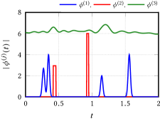
(a) Magnitude of the source element $\phi^{(j)}$.

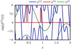
(b) Phase of the source element $\phi^{(j)}$.

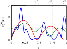
(c) Magnitude of the eigenfunction $u_{1}^{(j)}$.

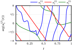
(d) Phase of the eigenfunction $u_{1}^{(j)}$.

Figure 2: Numerical construction of norm-minimizing solutions $u^{\dagger}\coloneqq u_{1}^{(j)}$ satisfying the source condition in Proposition 30 on the basis of an explicitly known source element $\phi^{(j)}$. For the approximation of the integral operator $\Phi_{\mathcal{I}_{k}^{*}[\phi]}$ in (30), a discretization with $N=10^{5}$ samples has been used.

6.2 Validation of the theoretical converence rate

To verify the convergence rate numerically, we have to solve the deautoconvolution problem for different noise levels. Referring to [Ger11] and [GHB⁺14], we here apply the Gauß-Newton method to the discretized problem with forward operator

$$\mathcal{A}_{k}[u]\bigl{(}\tfrac{n}{N}\bigr{)}\approx\frac{1}{N}\sum_{k=0}^{N}u\bigl{(}\tfrac{k}{N}\bigr{)}\,u\bigl{(}\tfrac{n-k}{N}\bigr{)}.$$

In order to solve the occurring equation systems iteratively, we use the conjugate gradient method with a suitable preconditioner and exploit the Toeplitz structure of the related system matrix, see for instance [RZR12]. For the exact signal $u^{\dagger}$ arising from the source element $\phi^{(3)}$, the numerical approximations $u^{*}_{j}$ corresponding to the minimizer $u_{\alpha}^{\delta}$ of the regularized and non-regularized deautoconvolution problem are shown in Figure 3. Besides the numerical ill-posedness of the discretized deautoconvolution problem for minor levels $\delta\coloneqq||\hskip 1.0ptg^{\delta}-g^{\dagger}\hskip 1.0pt||$ of Gaußian noise, we can here see the smoothing effect of the applied Tikhonov regularization. Even for considerably higher noise levels like $\delta=100||\hskip 1.0ptu^{\dagger}\hskip 1.0pt||$, the reconstruction covers the main features of the unknown norm-minimizing solution $u^{\dagger}$. The considered noise level $\delta$ here depends on the norm $||\hskip 1.0ptu^{\dagger}\hskip 1.0pt||$ of the true signal and not on the norm $||\hskip 1.0ptg^{\dagger}\hskip 1.0pt||$ of the exact data. Depending on our underlying numerical implementation, for the considered signal, the noise level $\delta=100||\hskip 1.0ptu^{\dagger}\hskip 1.0pt||$ corresponds to a Gaußian noise, whose norm approximately equals $||\hskip 1.0ptg^{\dagger}\hskip 1.0pt||$.

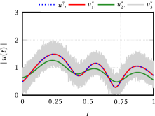
(a) Magnitude of the approximation $u^{*}_{j}$.

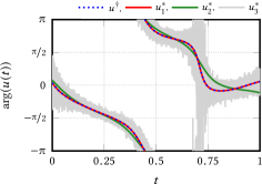
(b) Phase of the approximation $u^{*}_{j}$.

Figure 3: Comparison between the norm-minimizing solution $u^{\dagger}$ and the numerically reconstructed signals $u_{\alpha}^{\delta}$ with and without regularization. The noise level for $u^{*}_{1}$ and $u^{*}_{3}$ amounts to $\delta=0.05||\hskip 1.0ptu^{\dagger}\hskip 1.0pt||$, and for $u^{*}_{2}$ to $\delta=100||\hskip 1.0ptu^{\dagger}\hskip 1.0pt||$. The regularization for $u^{*}_{1}$ and $u^{*}_{2}$ corresponds to $\alpha=100\delta$. The reconstruction $u^{*}_{3}$ is computed without regularization or with $\alpha=0$.

Unfortunately, the result of the Gauß-Newton method usually strongly depends on the start value, which have to be a very accurate approximation of the norm-minimizing solution $u^{\dagger}$ for very low noise levels $\delta$. For this reason, we extent the simulations for the convergence rate analysis by choosing 25 randomly created start values around the true solution $u^{\dagger}$ per noise level. Since we have constructed the norm-minimizing solution $u^{\dagger}$ and the exact data $g^{\dagger}$ from a specific source element $\phi$, besides the convergence rates in Proof 30, we have an explicit upper bound for the Bregman distance between the regularized solution $u_{\alpha}^{\delta}$ and the norm-minimizing solution $u^{\dagger}$ as well as for the discrepancy between the forward operator $\mathcal{A}_{k}[u_{\alpha}^{\delta}]$ and the perturbed data $g^{\delta}$. The convergence rate analysis for the source element $\phi^{(3)}$ is presented in Figure 4. Additionally, Proof 30 yields an upper bound for the distance $||\hskip 1.0ptP_{E_{1}^{\perp}}(u_{\alpha}^{\delta})\hskip 1.0pt||^{2}=||\hskip 1.0ptu_{\alpha}^{\delta}-P_{E_{1}}(u_{\alpha}^{\delta})\hskip 1.0pt||^{2}$ between $u_{\alpha}^{\delta}$ and the ray $E_{1}$ spanned by $u^{\dagger}$. Here all three theoretical convergence rates and upper bounds match with numerical results.

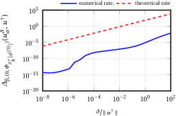
(a) Bregman distance between $u_{\alpha}^{\delta}$ and $u^{\dagger}$.

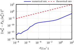
(b) Distance of $u_{\alpha}^{\delta}$ to ray $E_{1}$ spanned by $u^{\dagger}$.

(c) Discrepancy between $\mathcal{A}_{k}[u_{\alpha}^{\delta}]$ and $g^{\delta}$.

(d) Uncovered error part of $u_{\alpha}^{\delta}$ within the ray $E_{1}$ spanned by $u^{\dagger}$.

Figure 4: Comparison of the theoretical convergence rates in Corollary 30 and Theorem 30 with the numerical convergence rates for the source element $\phi^{(3)}$.

If we consider the discrepancy $||\hskip 1.0pt\mathcal{A}_{k}[u_{\alpha}^{\delta}]-g^{\delta}\hskip 1.0pt||$ in Figure 4.LABEL:sub@fig:conv-rate-ana:c more closely, we notice that the numerical and the theoretical rates coincides except for a multiplicative constant. Consequently, we cannot hope to improve the theoretical rate of $\mathop{\kern 0.0pt\mathcal{O}}\nolimits(\delta)$. The Bregman distance and the distance to the ray spanned by $u^{\dagger}$ have a completely different behaviour. More precisely, we here have regions where the convergence rate is faster and regions where the convergence rate is slower than the theoretical rate of $\mathop{\kern 0.0pt\mathcal{O}}\nolimits(\delta)$. Especially for the distance to the ray, it seems that the overall convergence rate is much faster than the theoretical rate. In some circumstances, our theoretical rate could thus be too pessimistic.

In this instance of the deautoconvolution problem, we can observe that the error $||\hskip 1.0ptP_{E_{1}}(u_{\alpha}^{\delta}-u^{\dagger})\hskip 1.0pt||^{2}=||\hskip 1.0ptu_{\alpha}^{\delta}-P_{E_{1}}(u_{\alpha}^{\delta})\hskip 1.0pt||^{2}$ within the ray $E_{1}$, which is not covered by Proof 30, numerically converges to zero superlinearly with a rate of $\mathop{\kern 0.0pt\mathcal{O}}\nolimits(\delta^{2})$. The shown numerical rate here strongly depends on the starting values of the Gauß-Newton method, which have been chosen in a small neighbourhood around $u^{\dagger}$. Choosing starting values around $-u^{\dagger}$, we would observe the same convergence rate to $-u^{\dagger}$. In fact, the sequence $u_{\alpha}^{\delta}$ could be composed of two subsequences – one converging to $u^{\dagger}$ and the other to $-u^{\dagger}$.

7 Conclusion

Starting from the question: how non-linear may a non-linear forward operator be in order to extend the linear regularization theory, we have introduced the classes of dilinear and diconvex mappings, which corresponds to linear, bilinear, and quadratic inverse problems. Exploiting the tensorial structure behind these mappings, we have introduced two different concepts of generalized subgradients and subdifferentials – the dilinear and the representative generalization. We have shown that the classical subdifferential calculus can be partly transferred to both new settings. Although the representative generalization yields stronger computation rules, the related subdifferential unfortunately strongly depends on the non-unique convex representative of the considered diconvex mapping. Besides all differences, there exists several connections between the dilinear and representative subdifferential.

On the basis of these preliminary considerations, we have examined the class of dilinear inverse problems. Analogously to linear inverse problems, the regularizations in the dilinear setting are well posed, stable, and consistent. Using the injective tensor product, which is nearly a predual space of the projective tensor product, as topologizing family, we have seen that the required sequential weak$*$ (semi-)continuity of the forward operator and regularization term may be inherited from the lifted versions. Moreover, we have derived a convergence rate analysis very similar to the linear setting under similar assumptions and requirements. This enables us to give explicit upper bounds for the discrepancy and the Bregman distance between the solution of the regularized problem and the $R$-minimizing solution.

In a last step, we have applied the developed theory to the deautoconvolution problem that appears in spectroscopy, optics, and stochastics. Although the requirements of the non-linear regularization theory are not fulfilled, our novel approach yields convergence rates based on a suitable range source condition and the dilinear Bregman distance. Depending on the source element, the Bregman distance is here surprisingly strong. In the best case, the solutions of the regularized problems converge strongly to the ray spanned by the true signal, which is the best possible rate with respect to the ambiguities of the problem. Using numerical experiments, we have considered different source elements and the corresponding norm-minimizing solutions, which shows that there exists signals satisfying the required source-wise representation. Finally, we have observed the established error bounds in the numerical simulations.

Acknowledgements.  We gratefully acknowledges the funding of this work by the Austrian Science Fund (FWF) within the project P28858. The Institute of Mathematics and Scientific Computing of the University of Graz, with which the authors are affiliated, is a member of NAWI Graz (http://www.nawigraz.at/).

References

• [1]
• [ABHS16] Anzengruber, Stephan W. ; Bürger, Steven ; Hofmann, Bernd ; Steinmeyer, Günter: Variational regularization of complex deautoconvolution and phase retrieval in ultrashort laser pulse characterization. In: Inverse Problems 32 (2016), No. 3, pp. 035002(27)
• [BB98] Bertero, Mario ; Boccacci, Patrizia: Introduction to Inverse Problems in Imaging. Bristol : Institute of Physics Publishing, 1998
• [BBM+04] Blaimer, M. ; Breuer, F. ; Mueller, M. ; Heidemann, R. M. ; Griswold, M. A. ; Jakob, P. M.: SMASH, SENSE, PILS, GRAPPA: how to choose the optimal method. In: Topics in Magnetic Resonance Imaging 15 (2004), No. 4, pp. 233–236
• [BC11] Bauschke, Heinz H. ; Combettes, Patrick L.: Convex Analysis and Monotone Operator Theory in Hilbert Spaces. New York : Springer, 2011 (CMS Books in Mathematics)
• [BFH16] Bürger, Steven ; Flemming, Jens ; Hofmann, Bernd: On complex-valued deautoconvolution of compactly supported functions with sparse Fourier representation. In: Inverse Problems 32 (2016), No. 10, pp. 104006(12)
• [BG94] Bakushinsky, A. ; Goncharsky, A.: Ill-posed Problems: Theory and Applications. Dordrecht : Kluwer Academic Publishers, 1994 (Mathematics and its Applications 301)
• [BH15] Bürger, Steven ; Hofmann, Bernd: About a deficit in low-order convergence rates on the example of autoconvolution. In: Applicable Analysis 94 (2015), No. 3, pp. 477–493
• [BL11] Bredies, Kristian ; Lorenz, Dirk: Mathematische Bildverarbeitung : Einführung in Grundlagen und moderne Theorie. Wiesbaden : Vieweg+Teubner, 2011
• [BO04] Burger, Martin ; Osher, Stanley: Convergence rates of convex variational regularization. In: Inverse Problems 20 (2004), No. 5, pp. 1411–1421
• [BS01] Burger, Martin ; Scherzer, Otmar: Regularization methods for blind deconvolution and blind source separation problems. In: Mathematics of Control, Signals and Systems 14 (2001), No. 4, pp. 358–383
• [CL05] Choi, Kerkil ; Lanterman, Aaron D.: An iterative deautoconvolution algorithm for nonnegative functions. In: Inverse Problems 21 (2005), No. 3, pp. 981–995
• [DF87] Dainty, J. C. ; Fienup, J. R.: Phase retrieval and image reconstruction for astronomy. In: Stark, Henry (Ed.): Image Recovery : Theory and Application. Orlando (Florida) : Academic Press, 1987, Chapter  7, pp. 231–275
• [DF93] Defant, Andreas ; Floret, Klaus: Tensor Norms and Operator Ideals. Amsterdam : North-Holland, 1993 (North-Holland Mathematics Studies 176)
• [DFS08] Diestel, Joe ; Fourie, Jan H. ; Swart, Johan : Grothendieck’s Résumé Revisited: The Metric Theory of Tensor Products. Providence, Rhode Island : American Mathematical Society, 2008
• [DL08] Dai, Zhewei ; Lamm, Patricia K.: Local regularization for the nonlinear inverse autoconvolution problem. In: SIAM Journal on Numerical Analysis 46 (2008), No. 2, pp. 832–868
• [EHN96] Engl, Heinz W. ; Hanke, Martin ; Neubauer, Andreas: Mathematics and Its Applications. Vol. 375: Regularization of Inverse Problems. Dortrecht : Kluwer Academic Publishers, 1996
• [EKN89] Engl, Heinz W. ; Kunisch, Karl ; Neubauer, Andreas: Convergence rates for Tikhonov regularisation of non-linear ill-posed problems. In: Inverse Problems 5 (1989), No. 4, pp. 523–540
• [ET76] Ekeland, Ivar ; Temam, Roger: Convex Analysis and Variational Problems. Amsterdam : North-Holland Publishing Company, 1976 (Studies in Mathematics and Its Applications 1)
• [FH96] Fleischer, Gunter ; Hofmann, Bernd: On inversion rates for the autoconvolution equation. In: Inverse Problems 12 (1996), No. 4, pp. 419–435
• [FL12] Fischer, Wolfgang ; Lieb, Ingo: A Course in Complex Analysis : From Basic Results to Advanced Topics. Wiesbaden : Vieweg+Teubner, 2012
• [Fle14] Flemming, Jens: Regularization of autoconvolution and other ill-posed quadratic equations by decomposition. In: Journal of Inverse and Ill-Posed Problems 22 (2014), No. 4, pp. 551–567
• [Ger11] Gerth, Daniel: Regularization of an autoconvolution problem occurring in measurements of ultra-short laser pulses. Chemnitz, Technische Universität Chemnitz, Diploma thesis, September 2011
• [GH94] Gorenflo, Rudolf ; Hofmann, Bernd: On autoconvolution and regularization. In: Inverse Problems 10 (1994), No. 2, pp. 353–373
• [GHB+14] Gerth, Daniel ; Hofmann, Bernd ; Birkholz, Simon ; Koke, Sebastian ; Steinmeyer, Günter: Regularization of an autoconvolution problem in ultrashort laser pulse characterization. In: Inverse Problems in Science and Engineering 22 (2014), No. 2, pp. 245–266
• [Gra10] Grasmair, Markus: Generalized Bregman distances and convergence rates for non-convex regulatization methods. In: Inverse Problems 26 (2010), No. 11, pp. 115014(16)
• [Gra11] Grasmair, Markus: Linear convergence rates for Tikhonov regularization with positively homogeneous functionals. In: Inverse Problems 27 (2011), No. 7, pp. 075014(16)
• [HKPS07] Hofmann, B. ; Kaltenbacher, B. ; Pöschl, C. ; Scherzer, O.: A convergence rates result for Tikhonov regularization in Banach spaces with non-smooth operators. In: Inverse Problems 23 (2007), No. 3, pp. 987–1010
• [Hof86] Hofmann, Bernd: Regularization for applied inverse and ill-posed problems. Leipzig : BSB B. G. Teubner Verlagsgesellschaft, 1986 (Teubner-Texte zur Mathematik 85)
• [IJ15] Ito, Kazufumi ; Jin, Bangti: Series on Applied Mathematics. Vol. 22: Inverse Problems : Tikhonov Theory and Algorithms. New Jersey : World Scientific, 2015
• [Jan00] Janno, Jaan: Lavrent’ev regulatization of ill-posed problems containing nonlinear near-to-monotone operators with applications to autoconvolution equation. In: Inverse Problems 16 (2000), No. 2, pp. 333–348
• [JR06] Justen, L. ; Ramlau, R.: A non-iterative regularization approach to blind deconvolution. In: Inverse Problems 22 (2006), No. 3, pp. 771–800
• [Lax02] Lax, Peter D.: Functional Analysis. New York : Wiley-Interscience. John Wiley & Sons, 2002 (Pure and Applied Mathematics)
• [Lic66] Lichnerowicz, A.: Einführung in die Tensoranalysis. Mannheim : Bibliographisches Institut, 1966 (BI-Hochschultaschenbücher 77*)
• [Lou89] Louis, Alfred K.: Inverse und schlecht gestellte Probleme. Stuttgart : B. G. Teubner, 1989 (Teubner Studienbücher Mathematik)
• [LP13] Lu, Shuai ; Pereverzev, Sergei V.: Regularization theory for ill-posed problems. Berlin : De Gruyter, 2013 (Inverse and Ill-posed Problems Series 58)
• [Meg98] Megginson, Robert E.: An Introduction to Banach Space Theory. New York : Springer, 1998 (Graduate Texts in Mathematics 183)
• [Mil90] Millane, R. P.: Phase retrieval in crystallography and optics. In: Journal of the Optical Society of America A 7 (1990), March, No. 3, pp. 394–411
• [Mor84] Morozov, V. A.: Methods for solving incorrectly posed problems. New York : Springer-Verlag, 1984
• [MS12] Mueller, Jennifer L. ; Siltanen, Samuli: Linear and Nonlinear Inverse Problems with Practical Applications. Philadelphia : SIAM, 2012 (Computational Science & Engineering)
• [Ram05] Ramm, Alexander G.: Inverse problems. Springer : Springer, 2005 (Mathematical and Analytical Techniques with Applications to Engineering)
• [Roc70] Rockafellar, R. Tyrrell: Convex Analysis. Princeton (New Jersey) : Princeton University Press, 1970 (Princeton Mathematical Series 28)
• [Rom08] Roman, Steven: Advanced Linear Algebra. 3rd Edition. New York : Springer, 2008 (Graduate Texts in Mathematics 135)
• [RS06] Resmerita, Elena ; Scherzer, Otmar: Error estimates for non-quadratic regularization and the relation to enhancement. In: Inverse Problems 22 (2006), No. 3, pp. 801–814
• [Rya02] Ryan, Raymond A.: Introduction to Tensor Products of Banach Spaces. London : Springer, 2002 (Springer Monographs in Mathematics)
• [RZR12] Redivo-Zaglia, Michela ; Rodriguez, Giuseppe: smt: a Matlab toolbox for structured matrices. In: Numerical Algorithms 59 (2012), No. 4, pp. 639–659
• [Sch11] Scherzer, Otmar (Ed.): Handbook of Mathematical Methods in Imaging. New York : Springer, 2011
• [SGG+09] Scherzer, Otmar ; Grasmair, Markus ; Grossauer, Harald ; Haltmeier, Markus ; Lenzen, Frank: Applied Mathematical Sciences. Vol. 167: Variational Methods in Imaging. New York : Springer, 2009
• [Sho97] Showalter, R. E.: Monotone Operators in Banach Space and Nonlinear Partial Differential Equations. Providence, Rhode Island : American Mathematical Society, 1997 (Mathematical Surveys and Monographs 49)
• [SKHK12] Schuster, Thomas ; Kaltenbacher, Barbara ; Hofmann, Bernd ; Kazimierski, Kamil S.: Regularization methods in Banach spaces. Berlin : de Gruyter, 2012 (Radon Series on Computational and Applied Mathematics 10)
• [SSD+06] Seifert, Birger ; Stolz, Heinrich ; Donatelli, Marco ; Langemann, Dirk ; Tasche, Manfred: Multilevel Gauss-Newton methods for phase retrieval problems. In: Journal of Physics. A. Mathematical and General 39 (2006), No. 16, pp. 4191–4206
• [SW13] Seo, Jin K. ; Woo, Eung J.: Nonlinear Inverse Problems in Imaging. Chichester : John Wiley & Sons, 2013
• [TA77] Tikhonov, A. N. ; Arsenin, V.: Solutions of Ill-Posed Problems. New York : John Wiley & Sons, 1977 (Scripta Series in Mathematics)
• [Tik63a] Tikhonov, A. N.: Regularization of incorrectly posed problems. In: Soviet Mathematics—Doklady 4 (1963), pp. 1624–1627. – Translation from Doklady Akademii Nauk SSSR 153, 49–52 (1963)
• [Tik63b] Tikhonov, A. N.: Solution of incorrectly formulated problems and the regularization method. In: Soviet Mathematics—Doklady 4 (1963), pp. 1035–1038. – Translation from Doklady Akademii Nauk SSSR 151, 501–504 (1963)
• [TLY98] Tikhonov, A. N. ; Leonov, A. S. ; Yagola, A. G.: Nonlinear ill-posed problems. Vol. 1, 2. London : Chapman & Hall, 1998 (Applied Mathematics and Mathematical Computation 14)
• [Uhl03] Uhlmann, Gunther (Ed.): Mathematical Sciences Research Institute Publications. Vol. 47: Inside Out: Inverse Problems and Applications. Cambridge : Cambridge University Press, 2003
• [Uhl13] Uhlmann, Gunther (Ed.): Mathematical Sciences Research Institute Publications. Vol. 60: Inverse Problems and applications: Inside Out II. Cambridge : Cambridge University Press, 2013
• [Wer02] Werner, Dirk: Funktionalanalysis. 4., überarbeitete Auflage. Berlin : Springer, 2002 (Springer-Lehrbuch)
• [Won79] Wong, Yau-Chuen: Schwartz Spaces, Nuclear Spaces and Tensor Products. Berlin : Springer-Verlag, 1979 (Lecture Notes in Mathematics 726)