Energy dependent topological adS black holes in Gauss–Bonnet Born–Infeld gravity

Abstract

Employing higher curvature corrections to Einstein–Maxwell gravity has garnered a great deal of attention motivated by the high energy regime in quantum nature of black hole physics. In addition, one may employ gravity’s rainbow to encode quantum gravity effects into the black hole solutions. In this paper, we regard an energy dependent static spacetime with various topologies and study its black hole solutions in the context of Gauss–Bonnet Born–Infeld (GB–BI) gravity. We study thermodynamic properties and examine the first law of thermodynamics. Using suitable local transformation, we endow the Ricci–flat black hole solutions with a global rotation and study the effects of rotation on thermodynamic quantities. We also investigate thermal stability in canonical ensemble through calculating the heat capacity. We obtain the effects of various parameters on the horizon radius of stable black holes. Finally, we discuss second order phase transition in the extended phase space thermodynamics and investigate the critical behavior.

I Introduction

James Clark Maxwell is one of the physicists who played the most decisive part in developing the electrodynamics. He collected and modified four equations that are known as the Maxwell’s equations, which are the foundation of classical electromagnetism. Maxwell electrodynamics contains various problems which motivate one to consider nonlinear electrodynamics (NED). One of the main problematic aspects of Maxwell theory is having an infinite self–energy for a point–like charge. To remove such divergency, Born and Infeld introduced one of the interesting theories of NED which is identified as Born–Infeld (BI) theory BI1 ; BI2 . Recently, such nonlinear theory has acquired a new impetus, since it can be naturally arisen in the low–energy limit of the open string theory BIstring1 ; BIstring2 ; BIstring3 ; BIstring4 ; BIstring5 .

On the gravitational point of view, Einstein gravity is a traditional theory of general relativity. Although such theory is successful for various aspects and is consistent with some observational evidences, it has some problems in higher curvature regimes. The natural extension of Einstein gravity is to consider the higher curvature gravity which is appeared as next-to-leading term in heterotic string effective action. Keeping quadratic curvature terms (and ignoring higher curvature terms) in such stringy effective action GBstring1 ; GBstring2 ; GBstring3 ; GBstring4 ; GBstring5 ; GBstring6 ; GBstring7 leads to the Gauss–Bonnet (GB) Lagrangian which is a topological invariant in four dimensions. Various aspects of GB gravity and its thermodynamic properties have been investigated in several papers GBpapers1 ; GBpapers2 ; GBpapers3 ; GBpapers4 ; GBpapers5 ; GBpapers6 ; GBpapers7 ; GBpapers8 ; GBpapers9 ; GBpapers10 ; GBpapers11 ; GBpapers12 ; GBpapers13 ; GBpapers14 ; GBpapers15 ; GBpapers16 ; GBpapers17 ; GBpapers18 ; GBpapers19 .

The electromagnetic and gravitational fields near the charged black holes are very strong, and hence, both the nonlinear electromagnetic effects and higher curvature gravitational terms should be taken into consideration. In other words, Maxwell theory and Einstein gravity can be, respectively, considered as approximations of NED theory and higher curvature gravity in the weak fields limit. Regarding the mentioned subjects, one is motivated to provide an analytically solvable theory which contains higher curvature corrections of gauge–gravity theories. Among generalizations of the Einstein–Maxwell action to a higher curvature gauge–gravity theory, the GB–BI gravity has some particular interests because it is a ghost-free theory in the gravitational side and a divergence-free field in the electromagnetic side. In addition, both GB and BI theories emerge in the effective low-energy action of string theory BIstring1 ; BIstring2 ; BIstring3 ; BIstring4 ; BIstring5 ; GBstring1 ; GBstring2 ; GBstring3 ; GBstring4 ; GBstring5 ; GBstring6 ; GBstring7 . The influences of GB gravity and BI theory have been investigated in various physical phenomena GBeffects1A ; GBeffects1B ; GBeffects1C ; GBeffects2A ; GBeffects2B ; GBeffects3 ; GBeffects4 ; GBeffects5A ; GBeffects5B ; GBeffects6A ; GBeffects6B ; BIsuperconductor1 ; BIsuperconductor2 ; BIsuperconductor3 ; BIHydrogen1 ; BIHydrogen2 ; BIHydrogen3 ; BIHawRad ; BIHydrodynamics ; BICosmology1 ; BICosmology2 ; BICosmology3 . Moreover, in the subject of black hole physics, various properties of GB–BI solutions were studied (for a very incomplete list of references, see GBBI1A ; GBBI1B ; GBBI2 ).

On the other hand, regarding high energy regime of gravitational physics, it is important to find the UV generalization of general relativity. There are various attempts to obtain the UV completion of general relativity, in which they should reduce to the general relativity in the IR limit. One of approaches for obtaining the UV completion of general relativity is based on the deformation of the usual energy-momentum dispersion relation in the UV limit, which is called gravity’s rainbow Grb . Considering gravity’s rainbow, one finds that the geometry of spacetime is made energy dependent through the introduction of rainbow functions Hendi-FaizalA ; Hendi-FaizalB .

On the other hand, one of the fundamental challenging subjects in cosmology is big bang singularity. It is shown that nonlinear electrodynamics can remove both the black hole and big bang singularities Nonsingular-nonlinearA ; Nonsingular-nonlinearB ; Nonsingular-nonlinearC ; Nonsingular-nonlinearD ; Nonsingular-nonlinearE . Besides, one can construct a nonsingular universe by considering an effective energy dependent spacetime NonsingularRainbow1 ; NonsingularRainbow2 ; NonsingularRainbow3 ; NonsingularRainbow4 ; NonsingularRainbow5 . In addition, an isotropic perfect fluid model is considered in the context of gravity’s rainbow to obtain a nonsingular bouncing universe NonsingularCosmology1 ; NonsingularCosmology2 . Moreover, the absence of singular black holes at the LHC is explained with the formalism of gravity’s rainbow NonsingularLHC . In other words, gravity’s rainbow is an effective approach for helping us to avoid the mentioned singularities.

It was shown that for a certain choice of rainbow functions, there is a close relation between gravity’s rainbow and Horava-Lifshitz gravity Rb-Lf . In addition, one may regard string theory motivation of considering gravity’s rainbow. The background fluxes in string theory produce a noncommutative deformation of the geometry Noncom1A ; Noncom1B , and such noncommutativity has also been used to motivate one of the most important classes of rainbow functions in gravity’s rainbow Noncom2A ; Noncom2B . Also, applying the spontaneous breaking of the Lorentz symmetry, one should use a deformation of the usual energy-momentum relations, and such modification can be used as a motivation for introducing gravity’s rainbow SSLB .

It is worthwhile to mention that if the energy of the particle, $E$, was just a non-dynamical parameter, one could gauge it away by rescaling. However, it dynamically depends on the coordinates and it does break original the diffeomorphisms symmetry of the full metric. In fact, even the local symmetry in gravity’s rainbow is not Lorentz symmetry, as it is based on modified dispersion relation. An explicit form of coordinate dependence of the energy for a particular solution was discussed in Ref. Rb-Lf . Although it is hard to find explicit dependence of the energy on the coordinates for various solutions, it is important to know that $E$ is a dynamical parameter and cannot be gauged away by rescaling.

After discovering the fact that the Hawking temperature and entropy are, respectively, proportional to black hole’s surface gravity and the area of its event horizon, investigation of black hole thermodynamics becomes a very interesting subject. In addition, regarding the cosmological constant as a dynamical pressure, one can study the critical behavior of a system in the extended phase space. In this regard, one finds an analogy between van der Waals liquid–gas system and the black hole as a thermodynamical system (for an incomplete references, see PressureLambda1 ; PressureLambda2 ; PressureLambda3 ; PressureLambda4 ; PressureLambda5 ; PressureLambda6 ; PressureLambda7 ; PressureLambda8 ; PressureLambda9 ; PressureLambda10 ; PressureLambda11 ).

The main goal of this paper is to find topological black hole solutions of the GB–BI gravity with an energy dependent spacetime. Although the system seems to be complex, as we mentioned, considering each item is based on a fundamental theory. It is worth mentioning that all higher curvature gravity, higher dimensional physics, higher curvature terms in gauge theory, and the existence of upper limit for the energy of a particle can be originated from heterotic string theory and modified dispersion relation, which are two fundamental acceptable theories. In this paper, we consider most important theory as well as simplest ones. In other words, between all higher curvature gravity (such as higher orders of Lovelock gravity and also $F(R)$ gravity theories), we select Gauss-Bonnet gravity which is the simplest second order derivative theory. On the other hand, regarding various models of nonlinear electrodynamics, we take into account the most interesting theory which has acceptable results. Regarding this theory, we could solve some problematic subjects from field theory to cosmological scales. Furthermore, regarding an energy dependent line element is the simplest way for considering the energy of particles on the geometry of spacetime. Hence, in this paper, we try to combine some interesting subjects, while we take care for the simplicity. We also discuss thermodynamic properties of such static topological black holes and generalize Ricci–flat adS solutions to rotating black branes. We show that how thermodynamical properties and possible phase transition of black hole can be affected by the higher-order curvature terms of gauge/gravity fields and the energy at which spacetime is probed. In other words, we study thermal stability and analyze the effects of GB, BI, rotation parameters and rainbow functions on stability criteria.

II Topological Black Hole Solutions

In this section, we are going to obtain $d-$dimensional black hole solutions with various horizon topologies. In the context of gravity’s rainbow, one may introduce a one-parameter family of energy dependent orthonormal frame field. As a result, one-parameter family of energy dependent metric has been created such as $g^{\mu\nu}(\varepsilon)=e_{a}^{\mu}(\varepsilon)e^{a\nu}(\varepsilon)$ where $\varepsilon=E/E_{p}$ is the energy ratio Grb . In this relation, $E$ and $E_{p}$, are respectively, the energy of test particle and Planck energy. At the first step, we consider the following energy dependent spherically symmetric line element:

$$d\tau^{2}=-ds^{2}=A(r,\varepsilon)dt^{2}-B(r,\varepsilon)dr^{2}-C(r,\varepsilon)d\Omega_{k}^{2},$$ (1)

where $A(r,\varepsilon)$, $B(r,\varepsilon)$ and $C(r,\varepsilon)$ are functions of energy and radial coordinate. In addition, $d\Omega_{k}^{2}$ indicates the Euclidian metric of a $(d-2)-$dimensional hypersurface with constant curvature $(d-2)(d-3)k$ and volume $V_{d-2}$, where $k$ is a constant. Hereafter, we take $k=\pm 1,0$, without loss of generality. For more clarifications, we present the explicit form of $d\Omega_{k}^{2}$ as

$$d\Omega_{k}^{2}=\left\{\begin{array}[]{cc}d\theta_{1}^{2}+\sum\limits_{i=2}^{d-2}\prod\limits_{j=1}^{i-1}\sin^{2}\theta_{j}d\theta_{i}^{2}&k=1\\ \sum\limits_{i=1}^{d-2}d\phi_{i}^{2}&k=0\\ d\theta_{1}^{2}+\sinh^{2}\theta_{1}(d\theta_{2}^{2}+\sum\limits_{i=3}^{d-2}\prod\limits_{j=2}^{i-1}\sin^{2}\theta_{j}d\theta_{i}^{2})&k=-1\end{array}\right..$$ (2)

The energy dependent metric functions are considered to make a connection between these new tetrad fields and the usual frame fields $\tilde{e}_{a}^{\mu}$ in general relativity, $f(\varepsilon)e_{0}^{\mu}(\varepsilon)=\tilde{e}_{0}^{\mu}$ and $g(\varepsilon)e_{i}^{\mu}(\varepsilon)=\tilde{e}_{i}^{\mu}$, where $i$ is the spatial index and $f(\varepsilon)$ and $g(\varepsilon)$ are rainbow functions. We also expect to recover the general relativity in the IR limit, as $\lim_{\varepsilon\rightarrow 0}f(\varepsilon)=\lim_{\varepsilon\rightarrow 0}g(\varepsilon)=1$. Hereafter, we use the following separation of variable for simplicity and also consistency with the energy dependent modified dispersion relation

$$A(r,\varepsilon)=\frac{\psi(r)}{f(\varepsilon)^{2}},\;\;\;\;B(r,\varepsilon)=\frac{1}{\psi(r)g(\varepsilon)^{2}},\;\;\;\;C(r,\varepsilon)=\frac{r^{2}}{g(\varepsilon)^{2}},$$ (3)

where in the IR limit the Schwarzschild like metric is recovered. Although there are different models of the rainbow functions with various phenomenological motivations (see Ref. Hendi-FaizalA for more details), we try to present all analytical relations with closed form of rainbow functions. This general form may help us to follow the trace of temporal ($f(\varepsilon)$) and spatial ($g(\varepsilon)$) rainbow functions, separately. But for plotting the diagrams and other numerical analysis, we have to choose a class of rainbow functions with adjusting free parameters.

In order to discuss geometric properties, we should calculate scalar curvatures. Regarding the metric (1) with Eq. (3), it is easy to show that the Ricci and Kretschmann scalars are, respectively,

$$R = g(\varepsilon)^{2}\left[-\psi^{\prime\prime}(r)-2(d-2)\frac{\psi^{\prime}(r)}{r}+(d-2)(d-3)\frac{k-\psi(r)}{r^{2}}\right],$$ (4)

$$R_{\mu\nu\rho\sigma}R^{\mu\nu\rho\sigma} = g(\varepsilon)^{4}\left[\psi^{\prime\prime 2}(r)+2(d-2)\left(\frac{\psi^{\prime}(r)}{r}\right)^{2}+2(d-2)(d-3)\left(\frac{k-\psi(r)}{r^{2}}\right)^{2}\right],$$ (5)

where prime and double prime are the first and second derivatives with respect to $r$ , respectively. Calculating the other curvature invariants (such as Ricci square, Weyl square and so on), we find that they are functions of $\psi^{\prime\prime}$, $\psi^{\prime}/r$ and $(k-\psi)/r^{2}$ and therefore, it is sufficient to study the Kretschmann scalar for investigating the spacetime curvature. Regarding Eqs. (4) and (5), one finds the considerable effect of rainbow function on all terms of curvature scalars. This indicates that the curvature of spacetime can be related to the energy at which spacetime is probed.

Since gravity’s rainbow has considerable effects at UV regime, it may be motivated to consider high energy and quantum corrections of gravity and gauge fields. In this regard, we are interested in the GB gravity coupled to a nonlinear $U(1)$ gauge field.

In addition, we should note that the constants may depend on the scale at which a theory is probed renom . Such dependency is based on the renormalization group flow. Also, according to the supergravity solutions, one may expect to consider energy dependent constants. As a result, it is interesting to take into account energy dependent constants. The action under study is

$$I_{G}=-\frac{1}{16\pi}\int_{\mathcal{M}}d^{d}x\sqrt{-g}\left[R-2\Lambda(\varepsilon)+\alpha(\varepsilon)L_{GB}+L(\mathcal{F})\right]$$ (6)

where $\Lambda(\varepsilon)$ and $\alpha(\varepsilon)$ are, respectively, the energy dependent cosmological constant and GB parameter. In addition, $L_{GB}$ and $L(\mathcal{F})$ refer to the Lagrangians of GB and BI theories, which can be written as

$$L_{GB}=R_{\mu\nu\gamma\delta}R^{\mu\nu\gamma\delta}-4R_{\mu\nu}R^{\mu\nu}+R^{2},$$ (7)

$$L(\mathcal{F})=4\beta(\varepsilon)^{2}\left(1-\sqrt{1+\frac{\mathcal{F}}{2\beta(\varepsilon)^{2}}}\right),$$ (8)

where $\beta(\varepsilon)$ is called the BI parameter, $\mathcal{F}=F_{\mu\nu}F^{\mu\nu}$ is the Maxwell invariant, in which $F_{\mu\nu}=\partial_{[\mu}A_{\nu]}$ is the Faraday tensor and $A_{\mu}$ is the gauge potential. Taking into account the action (6) and using the variational principle, we can obtain the following field equations

$$G_{\mu\nu}^{(0)}+G_{\mu\nu}^{(1)}+ G_{\mu\nu}^{(2)}=\frac{1}{2}L(\mathcal{F})g_{\mu\nu}-2L_{\mathcal{F}}F_{\mu\lambda}F_{\nu}^{\;\lambda},$$ (10)

$$\nabla_{\mu}\left(L_{\mathcal{F}}F^{\mu\nu}\right)=0,$$

where $L_{\mathcal{F}}=\frac{dL(\mathcal{F})}{d\mathcal{F}}$, $G_{\mu\nu}^{(0)}=\Lambda(\varepsilon)g_{\mu\nu}$, $G_{\mu\nu}^{(1)}$ is the Einstein tensor and $G_{\mu\nu}^{(2)}$ is the divergence-free symmetric tensor of GB contribution

$$G_{\mu\nu}^{(2)}=-\alpha(\varepsilon)\left(4R^{\rho\sigma}R_{\mu\rho\nu\sigma}-2R_{\mu}^{\ \rho\sigma\lambda}R_{\nu\rho\sigma\lambda}-2RR_{\mu\nu}+4R_{\mu\lambda}R_{\text{ \ }\nu}^{\lambda}+\frac{L_{GB}}{2}g_{\mu\nu}\right).$$ (11)

Regarding the metric (1) with the field equations (10) and (10), we can obtain energy dependent metric function. At first, we start with a consistent gauge potential $A_{\mu}$ with the following form

$$A_{\mu}=\frac{h(r)}{f(\varepsilon)}\delta_{\mu}^{0}$$ (12)

The functional form of $h(r)$ can be obtained from Eq. (10)

$$h(r)=-\frac{q(\varepsilon)}{(d-3)r^{d-3}}\ \mathcal{H},$$ (13)

where

$$\mathcal{H} = {}_{2}F_{1}\left(\left[\frac{1}{2},\frac{d-3}{2d-4}\right],\left[\frac{3d-7}{2d-4}\right],-\eta\right),$$ (14)

$$\eta = \frac{g(\varepsilon)^{2}q(\varepsilon)^{2}}{\beta(\varepsilon)^{2}r^{2d-4}},$$ (15)

in which $q(\varepsilon)$ is an integration constant proportional to the electric charge and ${}_{2}F_{1}\left(\left[a,b\right],\left[c\right],x\right)$ is hypergeometric function. Using series expansion for large $r$ (or large $\beta(\varepsilon)$), we find that the gauge potential is well-behaved, asymptotically

$$\left.h(r)\right|_{\text{Large }r}=-\frac{q(\varepsilon)}{(d-3)r^{d-3}}+\frac{g(\varepsilon)^{2}q(\varepsilon)^{3}}{2(3d-7)\beta(\varepsilon)^{2}r^{3d-7}}+O\left(\frac{1}{\beta(\varepsilon)^{4}r^{5d-11}}\right).$$ (16)

Eq. (16) confirms that for large values of $r$ (or $\beta(\varepsilon)$), the dominant (first) term of $h(r)$ is the same as the gauge potential in $d$-dimensional linear Maxwell theory and other terms are the Maxwell corrections. It is also notable that the rainbow function affects the correction terms.

Inserting metric (1) into the gravitational field equations with obtained gauge potential, one finds the following nonzero components of Eq. (10)

$$e_{1} = \left[2\alpha(\varepsilon)(d-4)\frac{g(\varepsilon)^{2}}{r^{2}}\left[\psi(r)-k\right]-\frac{1}{d-3}\right]\frac{\psi^{\prime}(r)}{r}-\frac{\left[\psi(r)-k\right]}{r^{2}}$$ (17)

$$+(d-4)(d-5)\alpha(\varepsilon)g(\varepsilon)^{2}\left[\frac{\psi(r)-k}{r^{2}}\right]^{2}+\frac{4\beta(\varepsilon)^{2}(1-\sqrt{1+\eta})-2\Lambda(\varepsilon)}{(d-2)(d-3)g(\varepsilon)^{2}}=0,$$

$$e_{2} = \left[\frac{1}{(d-3)(d-4)}-2\alpha(\varepsilon)g(\varepsilon)^{2}\frac{\left[\psi(r)-k\right]}{r^{2}}\right]\psi^{\prime\prime}(r)-2\alpha(\varepsilon)g(\varepsilon)^{2}\left(\frac{\psi^{\prime}(r)}{r}\right)^{2}$$ (18)

$$-2\alpha(\varepsilon)g(\varepsilon)^{2}\left[2(d-5)\frac{\left[\psi(r)-k\right]}{r^{2}}-\frac{1}{\alpha(\varepsilon)(d-4)g(\varepsilon)^{2}}\right]\frac{\psi^{\prime}(r)}{r}+\frac{\left[\psi(r)-k\right]}{r^{2}}$$

$$-(d-5)(d-6)\alpha(\varepsilon)g(\varepsilon)^{2}\frac{\left[\psi(r)-k\right]^{2}}{r^{d-3}}+\frac{2\Lambda(\varepsilon)-4\beta(\varepsilon)^{2}\left(1-\frac{1}{\sqrt{1+\eta}}\right)}{(d-3)(d-4)g(\varepsilon)^{2}}=0.$$

It is a matter of calculation to show that the following metric function satisfies all field equations, simultaneously

$$\psi(r)=k+\frac{r^{2}}{2\alpha(\varepsilon)(d-4)(d-3)g(\varepsilon)^{2}}\left(1-\sqrt{\digamma(r)}\right)$$ (19)

with

$$\digamma(r) = 1+\frac{8(d-3)(d-4)\alpha(\varepsilon)}{(d-1)(d-2)}\left(\Lambda(\varepsilon)+\frac{(d-1)(d-2)m(\varepsilon)}{2r^{d-1}}-\Theta(r)\right),$$ (20)

$$\Theta(r) = 2\beta(\varepsilon)^{2}\left[\left(1-\sqrt{1+\eta}\right)+\frac{d-2}{d-3}\eta\mathcal{H}\right],$$ (21)

where $m(\varepsilon)$ is an integration constant. For large values of nonlinearity parameter ($\beta(\varepsilon)\rightarrow\infty$), this solution reduces to GB-Maxwell gravity’s rainbow black hole Hendi-FaizalA . In addition, obtained solutions reduce to GB-BI black holes for IR limit $f(\varepsilon)=g(\varepsilon)=1$.

Using series expansion of metric function for large distance, we find that the dominant term is proportional to cosmological constant. Therefore, obtained solutions are asymptotically (a)dS with an effective cosmological constant (see Ref. GBBI2 for more details). Depending on the free parameters, one finds that the function $\digamma(r)$ may be positive, zero or negative. In order to obtain real (physical) solutions, we can use one of the following two methods. First, we can limit ourselves to the set of parameters, which lead to non-negative $\digamma(r)$ for $0\leq r<\infty$. Second, we can define $r_{R}$ as the largest root of $\digamma(r=r_{R})=0$, in which $\digamma(r)$ is positive for $r>r_{R}$. One can use suitable coordinate transformation ($r\longrightarrow r^{\prime}$) to obtain real solutions for $0\leq r^{\prime}<\infty$ (see the last reference in GBBI2 for more details). Hereafter, we follow the first method.

Now, we focus on obtaining black hole solutions. Inserting Eq. (19) in Eqs. (4) and (5), we find that both the Kretschmann and Ricci scalars diverge at $r=0$ and are finite for $r\neq 0$. Since there is at least one real positive root for the metric function, the mentioned singularity can be covered with an event horizon, and therefore, the solutions can be interpreted as black holes. In order to discuss the type of horizon, we can follow Refs. HendiNON1 ; HendiNON2 . It was shown that there is a critical value for nonlinearity parameter, $\beta_{c}(\varepsilon)$, in which for $\beta(\varepsilon)<\beta_{c}(\varepsilon)$, the horizon geometry of nonlinear charged solutions behaves like Schwarzschild solutions and singularity is spacelike. For $\beta(\varepsilon)>\beta_{c}(\varepsilon)$, the horizon geometry is the same as Reissner–Nordström black hole and the singularity is timelike. The mentioned singularity is null for $\beta(\varepsilon)=\beta_{c}(\varepsilon)$ (see Fig. 1 for more details).

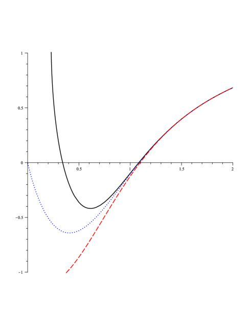
Figure 1: $\psi(r)$ versus $r$ for $k=1$, $d=5$, $g(\varepsilon)=f(\varepsilon)=0.95$, $\Lambda(\varepsilon)=-0.1$, $\alpha(\varepsilon)=0.1$, $q(\varepsilon)=1$, and $\beta(\varepsilon)>\beta_{c}(\varepsilon)$ (continuous line: timelike singularity), $\beta(\varepsilon)=\beta_{c}(\varepsilon)\approx 1.032$ (dotted line: null singularity) and $\beta(\varepsilon)<\beta_{c}(\varepsilon)$ (dashed line: spacelike singularity).

III Thermodynamics:

In this section, we discuss thermodynamical behavior of the black hole solutions. At first we calculate the Hawking temperature. To do so, we can use the surface gravity interpretation or follow the absence of conical singularity at the horizon in the Euclidean sector of the black hole solutions. Both methods lead to the following temperature

$$T=\frac{g(\varepsilon)}{4\pi f(\varepsilon)}\left.\frac{d\psi(r)}{dr}\right|_{r=r_{+}}.$$ (22)

After some manipulations, we obtain

$$T = \frac{r_{+}\left[\frac{4\beta(\varepsilon)^{2}\left[1-\sqrt{1+\eta_{+}}\right]-2\Lambda(\varepsilon)}{(d-2)}+\frac{(d-3)kg(\varepsilon)^{2}\left(1+\frac{k\alpha(\varepsilon)g(\varepsilon)^{2}}{r_{+}^{2}}(d-5)(d-4)\right)}{r_{+}^{2}}\right]}{4\pi f(\varepsilon)g(\varepsilon)\left[1+\frac{2k(d-3)(d-4)\alpha(\varepsilon)g(\varepsilon)^{2}}{r_{+}^{2}}\right]},$$ (23)

$$\eta_{+} = \left.\eta\right|_{r=r_{+}},$$

which shows that rainbow functions, the nonlinearity and GB parameters affect the black hole temperature.

Now, we are going to calculate entropy. Regarding Einstein gravity, it was shown that the entropy of black holes satisfies the so-called area law which states the black hole entropy is equal to one-quarter of horizon area Bekenstein1A ; Bekenstein1B ; Bekenstein1C ; Hawking1A ; Hawking1B . However, we could not use the area law for higher curvature gravity fails1 ; fails2 . It is known that the entropy in of asymptotically flat solutions ($\Lambda(\varepsilon)=0$) of GB gravity can be obtained from Wald formula Wald1 ; Wald2 ; Wald3 ; Wald4 ; Wald5

$$S=\frac{1}{4}\int d^{d-2}x\sqrt{\tilde{g}}\left(1+2\alpha(\varepsilon)\widetilde{R}\right)=\frac{r_{+}^{d-2}}{4g(\varepsilon)^{d-2}}\left(1+\frac{2k\left(d-2\right)(d-3)\alpha(\varepsilon)g(\varepsilon)^{2}}{r_{+}^{2}}\right),$$ (24)

where the integration is done on the $(d-2)$-dimensional spacelike hypersurface with the induced metric $\tilde{g}_{\mu\nu}$. We should note that $\tilde{g}$ is the determinant of $\tilde{g}_{\mu\nu}$ and $\tilde{R}$ is the Ricci scalar for the induced metric. Following Gibbs-Duhem relation, one can show that the entropy of asymptotically (a)dS black holes in GB gravity is the same as Eq. (24). It is notable that although the (nonlinear) electromagnetic source changes the locations of inner and outer horizons, it does not change the functional form of entropy formula and also area law (see Ref. entropyCharge for more details).

Calculating the flux of the electric field through a given closed hypersurface at infinity, one can obtain the electric charge per unit volume $V_{d-2}$ of the black hole, yielding

$$Q=\frac{q(\varepsilon)f(\varepsilon)}{4\pi g(\varepsilon)^{d-3}},$$ (25)

which shows that although the total charge does not depend on the nonlinearity of the electromagnetic field, it depends on the energy functions. This behavior is expected, since for large values of radial coordinate, the electric field of BI theory reduces to linear Maxwell field, but metric components depend on the energy functions. Regarding $\partial_{t}$ as the Killing vector ($\chi^{\mu}$) of static spacetime, we can obtain the electric potential of event horizon with respect to the potential reference

$$\Phi=A_{\mu}\chi^{\mu}\left|{}_{r\rightarrow\infty}-A_{\mu}\chi^{\mu}\right|_{r=r_{+}}=\frac{q(\varepsilon)\mathcal{H}_{+}}{(d-3)r_{+}^{d-3}},$$ (26)

where $\mathcal{H}_{+}=\mathcal{H}(r=r_{+})$.

Considering the behavior of the metric at large $r$, one can obtain the ADM (Arnowitt-Deser-Misner) mass of black hole for asymptotically flat solutions Brewin . In addition, we use the counterterm method to calculate the finite mass of (a)dS solutions. Both calculations (ADM and counterterm methods) lead to the following unique relation for the mass per unit volume $V_{d-2}$

$$M=\frac{(d-2)m(\varepsilon)}{16\pi f(\varepsilon)g(\varepsilon)^{d-1}}.$$ (27)

Since all conserved and thermodynamic quantities have been obtained, we can examine the validity of the first law of thermodynamics. Considering the expressions for the entropy, the electric charge and the mass given in Eqs. (24), (25) and (27), we can obtain the total mass $M$ as a function of the extensive quantities $Q$ and $S$, such as Smarr-type formula

$$M(S,Q)=\frac{f(\varepsilon)^{2}r_{+}^{d-1}}{16(d-1)}\left(\frac{4(d-2)\Omega\beta(\varepsilon)^{2}\mathcal{A}}{(d-3)}+4\beta(\varepsilon)^{2}(1-\sqrt{1+\Omega})-2\Lambda(\varepsilon)+\Sigma\right),$$ (28)

where $r_{+}=r_{+}(S)$ and

$$\Sigma = \frac{(d-1)(d-2)kg(\varepsilon)^{2}}{r_{+}^{2}}\left[1+\frac{(d-3)(d-4)k\alpha(\varepsilon)g(\varepsilon)^{2}}{r_{+}^{2}}\right],$$

$$\mathcal{A} = {}_{2}F_{1}\left(\left[\frac{1}{2},\frac{d-3}{2d-4}\right],\left[\frac{3d-7}{2d-4}\right],-\Omega\right),$$

$$\Omega = \frac{16\pi^{2}g(\varepsilon)^{2d-4}Q^{2}}{\beta(\varepsilon)^{2}f(\varepsilon)^{2}r_{+}^{2d-4}}.$$

Now, we regard $Q$ and $S$ as the extensive parameters and introduce their conjugate intensive parameters which are, respectively, the temperature and the electric potential, as

$$T=\left(\frac{\partial M}{\partial S}\right)_{Q}=\left(\frac{\partial M}{\partial r_{+}}\right)_{Q}\left/\left(\frac{\partial S}{\partial r_{+}}\right)_{Q}\right.,$$ (29)

$$\Phi=\left(\frac{\partial M}{\partial Q}\right)_{S}=\left(\frac{\partial M}{\partial q}\right)_{S}\left/\left(\frac{\partial Q}{\partial q}\right)_{S}\right..$$ (30)

It is straightforward to show that Eqs. (29) and (30) are equal to Eqs. (23) and (26), respectively, and therefore, one can conclude that these quantities satisfy the first law of thermodynamics

$$dM=TdS+\Phi dQ.$$ (31)

Now, we are going to check thermal stability. Thermodynamic stability of black holes can be investigated in various ensembles. Referring to thermal stability criterion in the canonical ensemble, stable black holes have positive heat capacity ($C_{Q}=T_{+}/\left(\partial^{2}M/\partial S^{2}\right)_{Q}$ ). As an additional note, we should mention that since size plays an essential role in gravitational thermodynamics, the negativity of the heat capacity does no, necessarily, mean that a system is unstable in the canonical ensemble. There are some finite size black hole systems with negative heat capacity but stable state York . Since the black hole systems, here, have infinite size, negative $C_{Q}$ indicates unstable state.

The canonical ensemble instability criterion is sufficiently strong to veto some gravity toy models. Thermal stability of a typical thermodynamic system should be considered as the result of small variations of the thermodynamic coordinates. In this regard, the energy $\mathcal{M}(S,Q)$ should be a convex function of its extensive variable. The electric charge is a fixed parameter in the canonical ensemble and the positivity of heat capacity is sufficient to ensure (local) thermal stability. After some calculations, we find

$$C_{Q}=\frac{(d-2)r_{+}^{d}\left[1+\frac{2(d-3)(d-4)k\alpha(\varepsilon)g(\varepsilon)^{2}}{r_{+}^{2}}\right]^{2}\left[2\Lambda(\varepsilon)-4\beta(\varepsilon)^{2}(1-\sqrt{1+\eta_{+}})-A_{0}\right]}{4(d-3)g(\varepsilon)^{d}\left[2(d-4)k\alpha(\varepsilon)A_{1}+(d-2)kA_{2}-\frac{4q(\varepsilon)^{2}\left(1+A_{3}\right)}{r_{+}^{2d-6}\sqrt{1+\eta_{+}}}\right]},$$ (32)

where

$$A_{0} = \frac{(d-2)(d-3)kg(\varepsilon)^{2}}{r_{+}^{2}}\left[1+\frac{(d-4)(d-5)\alpha(\varepsilon)kg(\varepsilon)^{2}}{r_{+}^{2}}\right],$$

$$A_{1} = \frac{(d-2)(d-3)kg(\varepsilon)^{2}}{r_{+}^{2}}\left(\frac{(d-4)(d-5)k\alpha(\varepsilon)g(\varepsilon)^{2}}{r_{+}^{2}}-1\right)-12\left(\beta(\varepsilon)^{2}-\frac{\Lambda(\varepsilon)}{2}\right),$$

$$A_{2} = 1+\frac{3(d-4)(d-5)k\alpha(\varepsilon)g(\varepsilon)^{2}}{r_{+}^{2}}-\frac{4r_{+}^{2}}{(d-2)(d-3)kg(\varepsilon)^{2}}\left(\beta(\varepsilon)^{2}-\frac{\Lambda(\varepsilon)}{2}\right),$$

$$A_{3} = \frac{2(d-4)(d-5)k\alpha(\varepsilon)g(\varepsilon)^{2}}{r_{+}^{2}}-\frac{\beta(\varepsilon)^{2}r_{+}^{2d-4}}{q(\varepsilon)^{2}}\left(\frac{1}{(d-3)g(\varepsilon)^{2}}+\frac{6(d-4)k\alpha(\varepsilon)}{r_{+}^{2}}\right).$$

It is a nontrivial task to analytically find the positivity of the heat capacity. Instead, we use the numerical analysis with various plots to discuss the sign and divergence points of heat capacity. Regarding Figs. 2–4 with selected parameters, one finds that two different cases may take place for the heat capacity.

$\begin{array}[]{cc}\epsfbox{Talpha.eps}&\epsfbox{Calpha.eps}\end{array}$

Figure 2: $T$ (left) and $C_{Q}$ (right) diagrams versus $r_{+}$ for $d=5$, $g(\varepsilon)=f(\varepsilon)=0.9$, $\Lambda(\varepsilon)=-1$, $\beta(\varepsilon)=0.1$, $q(\varepsilon)=0.1$, and $\alpha(\varepsilon)=0.05$ (continuous line), $\alpha(\varepsilon)=0.09$ (dotted line) and $\alpha(\varepsilon)=0.10$ (dashed line).

$\begin{array}[]{cc}\epsfbox{Tbeta.eps}&\epsfbox{Cbeta.eps}\end{array}$

Figure 3: $T$ (left) and $C_{Q}$ (right) diagrams versus $r_{+}$ for $d=5$, $g(\varepsilon)=f(\varepsilon)=0.9$, $\Lambda(\varepsilon)=-1$, $\alpha(\varepsilon)=0.07$, $q(\varepsilon)=0.3$, and $\beta(\varepsilon)=0.1$ (continuous line), $\beta(\varepsilon)=0.5$ (dotted line) and $\beta(\varepsilon)=1.0$ (dashed line).

$\begin{array}[]{cc}\epsfbox{Tfe.eps}&\epsfbox{Cfe.eps}\end{array}$

Figure 4: $T$ (left) and $C_{Q}$ (right) diagrams versus $r_{+}$ for $d=5$, $\Lambda(\varepsilon)=-1$, $\alpha(\varepsilon)=0.08$, $\beta(\varepsilon)=0.1$, $q(\varepsilon)=0.2$, and $f(\varepsilon)=g(\varepsilon)=0.8$ (continuous line), $f(\varepsilon)=g(\varepsilon)=1.0$ (dotted line) and $f(\varepsilon)=g(\varepsilon)=1.2$ (dashed line).

In the first case, $C_{Q}$ is positive definite for $r_{+}>r_{0}$, in which $r_{0}$ is the real positive root of temperature. Also, variation of free parameters in this case leads to changing $r_{0}$. In this regard, we study the effects of GB coefficient ($\alpha(\varepsilon)$), BI parameter ($\beta(\varepsilon)$) and rainbow function ($g(\varepsilon)$). Left panels of Figs. 2–4 and numerical analysis show that although variation of $\alpha(\varepsilon)$ does not have significant effect on $r_{0}$, and $r_{0}$ is an increasing function of $\beta(\varepsilon)$ (decreasing function of $g(\varepsilon)$).

In the second case, there are two divergence points ($r_{+1}$ and $r_{+2}$ with $r_{+1}<r_{+2}$ ) for the heat capacity. In other words, the heat capacity is positive for $r_{0}<r_{+}<r_{+1}$ and $r_{+}>r_{+2}$ and black hole is stable in these ranges. However, there is an unstable state for $r_{+1}<r_{+}<r_{+2}$. Considering phase space conception, one may consider a phase transition between the mentioned two stable states. It is worthwhile to mention that variation of free parameters may change the locations of $r_{+1}$ and $r_{+2}$. In addition, right panels of Figs. 2–4 indicate that the unstable range of event horizon is an increasing function of $g(\varepsilon)$ and a decreasing function of $\alpha(\varepsilon)$ and $\beta(\varepsilon)$. In other words, one can find a limit value for GB coefficient ($\alpha_{0}(\varepsilon)$) BI parameter ($\beta_{0}(\varepsilon)$) and rainbow function ($g_{0}(\varepsilon)$), in which for $\alpha(\varepsilon)>\alpha_{0}(\varepsilon)$ ($\beta(\varepsilon)>\beta_{0}(\varepsilon)$ or $g(\varepsilon)<g_{0}(\varepsilon)$), there is no unstable phase and the heat capacity is positive definite in the range of $r_{+}>r_{0}$.

IV Asymptotically adS rotating black branes

In this section, we are going to add a global rotation into the zero curvature horizon ($k=0$). The maximum number of independent rotation parameters is equal to $[\frac{d-1}{2}]$ ($[x]$ is the integer part of $x$) which is due to the fact that the rotation group in $d-$dimensions is $SO(d-1)$. Now, we perform the following local boost transformation in the $t-\phi_{i}$ planes for adding the angular momentum

$$\frac{t}{f(\varepsilon)}\mapsto\Xi(\varepsilon)\frac{t}{f(\varepsilon)}-a_{i}(\varepsilon)\frac{\phi_{i}}{g(\varepsilon)},\hskip 14.22636pt\frac{\phi_{i}}{g(\varepsilon)}\mapsto\Xi(\varepsilon)\frac{\phi_{i}}{g(\varepsilon)}-\frac{a_{i}(\varepsilon)}{l(\varepsilon)^{2}}\frac{t}{f(\varepsilon)},$$ (33)

where $l(\varepsilon)$ is an energy dependent scale parameter with length dimension, $a_{i}(\varepsilon)$ is rotation parameters in which $i=1...[\frac{d-1}{2}]$ and $\Xi(\varepsilon)=\sqrt{1+\sum_{i=1}^{p}\frac{a_{i}(\varepsilon)^{2}}{l(\varepsilon)^{2}}}$. Applying such boost into the metric (1) with $k=0$, one can obtain the following $d$-dimensional Ricci-flat solutions with $p\leq[\frac{d-1}{2}]$ rotation parameters

$$ds^{2} = -\psi(r)\left(\frac{\Xi(\varepsilon)}{f(\varepsilon)}dt-\frac{1}{g(\varepsilon)}{{\sum_{i=1}^{p}}}a_{i}(\varepsilon)d\phi_{i}\right)^{2}+\frac{r^{2}}{l^{4}}{{\sum_{i=1}^{p}}}\left(\frac{a_{i}(\varepsilon)}{f(\varepsilon)}dt-\frac{\Xi(\varepsilon)l(\varepsilon)^{2}}{g(\varepsilon)}d\phi_{i}\right)^{2}$$ (34)

$$\ \text{ }+\frac{dr^{2}}{g(\varepsilon)^{2}\psi(r)}-\frac{r^{2}}{g(\varepsilon)^{2}l(\varepsilon)^{2}}{\sum_{i<j}^{p}}[a_{i}(\varepsilon)d\phi_{j}-a_{j}(\varepsilon)d\phi_{i}]^{2}+\frac{r^{2}}{g(\varepsilon)^{2}}{{\sum_{i=p+1}^{d-2}}}d\phi_{i}^{2}.$$

Using Eq. (10), we can obtain the following consistent gauge potential

$$A_{\mu}=h(r)\left(\frac{\Xi(\varepsilon)}{f(\varepsilon)}\delta_{\mu}^{0}-\frac{a_{i}(\varepsilon)}{g(\varepsilon)}\delta_{\mu}^{i}\right)\text{ \ \ (no sum on }i\text{)}$$ (35)

where $h(r)$ is the same as Eq. (13). In addition, straightforward calculations show that all components of the gravitational field equation (10) can be satisfied by the metric function of Eq. (19). It is worthwhile to mention that the local transformation (33) generates a new metric, because it is not a proper coordinate transformation on the entire manifold Stachel . In other words, the static and rotating metrics can be locally mapped into each other but not globally, and therefore they are distinct.

Following the same method, one can find that there is a curvature singularity at $r=0$, which can be covered with an event horizon. Therefore, one may interpret such singularity as a black brane. Using the fact that $\chi=\partial_{t}+{\sum_{i}}\Omega_{i}\partial_{\phi_{i}}$ is the null generator of the horizon for the mentioned rotating black branes, we can obtain

$${T}_{rotating}{=}\left.\frac{{T}_{static}}{\Xi(\varepsilon)}\right|_{k=0},$$ (36)

$$\Phi_{rotating}{=}\frac{\Phi_{static}}{\Xi(\varepsilon)},$$ (37)

$$Q_{rotating}=\Xi(\varepsilon)Q_{static},$$ (38)

$$S_{rotating}=\left.\Xi(\varepsilon)S_{static}\right|_{k=0},$$ (39)

$$M_{rotating}=\left(\frac{(d-1)\Xi(\varepsilon)^{2}-1}{d-2}\right)M_{static},$$ (40)

and for rotating quantities, one can, respectively, obtain the following functional forms of angular velocities and angular momenta

$$\Omega_{i}=\frac{a_{i}(\varepsilon)}{\Xi(\varepsilon)l(\varepsilon)^{2}},$$ (41)

$$J_{i}=\frac{d-1}{16\pi}\Xi(\varepsilon)m(\varepsilon)a_{i}(\varepsilon).$$ (42)

In order to examine the validity of the first law of thermodynamics, we regard $S$, $Q$ and $J_{i}$’s as a complete set of extensive quantities for the mass $M(S,Q,J_{i})$ and define intensive quantities conjugate to them. The conjugate quantities are $T$, $\Phi$ and $\Omega_{i}$’s

$$T = \left(\frac{\partial\mathcal{M}}{\partial S}\right)_{Q,J_{i}},$$ (43)

$$\Phi = \left(\frac{\partial\mathcal{M}}{\partial Q}\right)_{S,J_{i}},$$ (44)

$$\Omega_{i} = \left(\frac{\partial\mathcal{M}}{\partial J_{i}}\right)_{S,Q}.$$ (45)

Considering the fact that metric function vanishes at the event horizon with Eqs. (43), (44) and (45), we find that the intensive quantities calculated by Eqs. (43), (44) and (45) are, respectively, consistent with Eqs. (36), (37) and (41), and therefore, one can confirm that the relevant thermodynamic quantities satisfy the first law of thermodynamics as

$$dM=TdS+\Phi dQ+\sum_{i}\Omega_{i}dJ_{i}.$$ (46)

Since we investigate thermodynamic stability of adS Ricci-flat static black holes in previous section. Here, we are going to check the effect of rotation on thermal stability. For rotating solutions, the mass $M$ is a function of the entropy $S$, the angular momentum $J$ and the electric charge $Q$. As we mentioned before, the positivity of the heat capacity $C_{Q,J}=T\left/\left(\partial^{2}M/\partial S^{2}\right)_{Q,J}\right.$ is sufficient to ensure the thermodynamic stability. Numerical calculations show that the effects of variation of rainbow functions, BI parameter and GB coefficient are the same as those in static case. In addition, as it was shown in Ref. GBBI2 , $C_{Q,J}$ is an increasing regular function of $\Xi$. Thus we ignore more explanations and in the next section, we focus on more interesting case $k=1$ for investigating critical behavior.

V Critical behavior

Here, we use the the extended phase space thermodynamics to investigate critical behavior. To do so, we take into account the adS black holes with spherical horizons (it was shown that there is not any van der Waals like phase transition for $k=0$ and $k=-1$). In this regard, we treat the cosmological constant as a thermodynamics pressure. In fact, we do not work in a fixed AdS background, and therefore, the cosmological constant is not a constant anymore, but a variable. If we treat the negative cosmological constant proportional to thermodynamic pressure, its conjugate quantity will be thermodynamic volume. Using the scaling argument, it has already been shown that the Smarr relation is consistent with first law of thermodynamics by assuming the cosmological constant as a thermodynamic variable. Here, we regard the following relation between the cosmological constant and the pressure PressureLambda1 ; PressureLambda2 ; PressureLambda3 ; PressureLambda4 ; PressureLambda5 ; PressureLambda6 ; PressureLambda7 ; PressureLambda8 ; PressureLambda9 ; PressureLambda10 ; PressureLambda11 )

$$P=-\frac{\Lambda(\varepsilon)}{{8\pi}}.$$ (47)

As a notable comment, it is worthwhile to mention that it was shown that the modified Smarr relation which can be calculated by the scaling argument is completely in agreement with the modified first law of thermodynamics in the extended phase space. In this regard, in addition to $\Lambda(\varepsilon)$, the nonlinearity parameter ($\beta(\varepsilon)$) and GB parameter ($\alpha(\varepsilon)$) are two other thermodynamical variables Smarr1 ; Smarr2 . It is notable that in the presence of rainbow functions, the modified first law of thermodynamics can be written as

$$dM=TdS+\Phi dQ+VdP+\mathcal{A}d\alpha+\mathcal{B}d\beta,$$ (48)

where the conjugate quantities can be obtained as

$$T = \left(\frac{\partial M}{\partial S}\right)_{Q,P,\alpha,\beta},$$

$$\Phi = \left(\frac{\partial M}{\partial Q}\right)_{S,P,\alpha,\beta},$$

$$V = \left(\frac{\partial M}{\partial P}\right)_{S,Q,\alpha,\beta},$$

$$\mathcal{A} = \left(\frac{\partial M}{\partial\alpha}\right)_{S,Q,P,\beta},$$

$$\mathcal{B} = \left(\frac{\partial M}{\partial\beta}\right)_{S,Q,P,\alpha}.$$

Moreover, we can obtain the generalized Smarr relation for our asymptotically adS solutions in the extended phase space

$$(d-3)M=(d-2)TS+(d-3)Q\Phi-2PV-2\left(\frac{d-2}{d-4}\right)\mathcal{A}\alpha-\mathcal{B}\beta,$$ (49)

which is completely in agreement with the mentioned modified first law of thermodynamics.

Inserting Eq. (47) in the temperature equation (23), one can find equation of state $P=P(T,r_{+})$

$$P = \frac{4\beta(\varepsilon)^{2}}{16\pi}\left(\sqrt{1+\eta_{+}}-1\right)+\left(1+\frac{2(d-3)(d-4)\alpha(\varepsilon)g(\varepsilon)^{2}}{r_{+}^{2}}\right)\frac{(d-2)f(\varepsilon)g(\varepsilon)T}{4r_{+}}-$$ (50)

$$\frac{(d-2)(d-3)g(\varepsilon)^{2}}{16\pi r_{+}^{2}}\left(1+\frac{(d-4)(d-5)\alpha(\varepsilon)g(\varepsilon)^{2}}{r_{+}^{2}}\right).$$

Since the critical point is an inflection point on the critical isothermal $P-r_{+}$ diagrams, we use the following relations to obtain the proper equations for critical quantities

$$\left(\frac{\partial P}{\partial r_{+}}\right)_{T}=0,$$ (51)

$$\left(\frac{\partial^{2}P}{\partial r_{+}^{2}}\right)_{T}=0.$$ (52)

Using Eqs. (51) and (52), one can find the critical quantities. Numerical calculations confirm that by choosing suitable parameters, one can find critical values for thermodynamic quantities. In order to analyze the effects of various parameters, we present different tables (see tables $1-6$). Accordingly, we can find that GB and nonlinearity parameters, rainbow functions and dimensionality affect the critical quantities. Based on tables $1$ and $2$, one finds increasing GB parameter leads to increasing critical volume and decreasing critical temperature and pressure. In addition, for sufficiently large $\alpha(\varepsilon)$, one can obtain the universality ratio $1/4$ independent of other parameters. It is notable that if we increase $\alpha(\varepsilon)$ more, we cannot obtain a real positive values for the critical quantities. In other words, there is an $\alpha_{0}(\varepsilon)$ in which for $\alpha(\varepsilon)>\alpha_{0}(\varepsilon)$ there is no phase transition and critical behavior (see Fig. 2 for more details). We should note that the value of $\alpha_{0}(\varepsilon)$ depends on other parameters. The same behavior takes place for the nonlinearity parameter. It means that critical volume is (critical temperature and pressure are) an increasing function (decreasing functions) of BI parameter, and also there is a $\beta_{0}(\varepsilon)$ in which for $\beta(\varepsilon)>\beta_{0}(\varepsilon)$ system is thermally stable and there is no phase transition (see Fig. 3 for more details). For the rainbow functions, we obtain different behavior. We find that by increasing these functions, all critical quantities are increasing, except critical temperature. In addition, there is a lower bound for the rainbow functions, in which if we regard the values of the rainbow functions less than such bound, we cannot find any phase transition (see Fig. 4 for more details).

$\alpha(\varepsilon)$     $r_{c}$     $T_{c}$     $P_{c}$     $\frac{P_{c}r_{c}}{T_{c}}$ $0.0100$ 0.4606 0.3456 0.1868 0.2490 $0.0500$ 0.8822 0.1807 0.0505 0.2468 $0.1000$ 1.2072 0.1328 0.0270 0.2458 $0.5000$ 2.6086 0.0636 0.0062 0.2561 $1.0000$ 3.5479 0.0456 0.0032 0.2528 $10.0000$ 10.9575 0.0145 0.0003 0.2500

$\alpha(\varepsilon)$     $r_{c}$      $T_{c}$      $P_{c}$     $\frac{P_{c}r_{c}}{T_{c}}$ $0.01000$ 0.6790 0.3720 0.1869 0.3411 $0.05000$ 1.1013 0.1938 0.0547 0.3106 $0.10000$ 1.4543 0.1410 0.0295 0.3048 $0.50000$ 2.0513 0.0647 0.0064 0.2041 $1.00000$ 3.2858 0.0459 0.0033 0.2367 $10.0000$ 10.9384 0.0145 0.0003 0.2496

Table $1$ (left): Critical values for $q(\varepsilon)=1$, $f(\varepsilon)=g(\varepsilon)=1$, $\beta(\varepsilon)=0.1$ and $d=5$.

Table $2$ (right): Critical values for $q(\varepsilon)=1$, $f(\varepsilon)=g(\varepsilon)=1$, $\beta(\varepsilon)=0.1$ and $d=6$.

$\beta(\varepsilon)$     $r_{c}$     $T_{c}$     $P_{c}$     $\frac{P_{c}r_{c}}{T_{c}}$ $0.0100$ 0.3566 0.4464 0.3130 0.2500 $0.0500$ 0.4000 0.3979 0.2485 0.2498 $0.1000$ 0.4606 0.3456 0.1868 0.2490 $0.5000$ 1.3362 0.1696 0.0365 0.2877 $1.0000$ 1.4922 0.1633 0.0335 0.3059 $10.0000$ 1.5265 0.1618 0.0328 0.3093

$\beta(\varepsilon)$     $r_{c}$     $T_{c}$     $P_{c}$     $\frac{P_{c}r_{c}}{T_{c}}$ $0.0100$ 0.2449 0.4332 0.2210 0.1250 $0.0500$ 0.5769 0.4055 0.2317 0.3296 $0.1000$ 0.6790 0.3720 0.1869 0.3411 $0.5000$ 1.2425 0.2764 0.0892 0.4010 $1.0000$ 1.3299 0.2708 0.0850 0.4170 $10.0000$ 1.3515 0.2693 0.0838 0.4205

Table $3$ (left): Critical values for $q(\varepsilon)=1$, $f(\varepsilon)=g(\varepsilon)=1$, $\alpha(\varepsilon)=10^{-2}$ and $d=5$.

Table $4$ (right): Critical values for $q(\varepsilon)=1$, $f(\varepsilon)=g(\varepsilon)=1$, $\alpha(\varepsilon)=10^{-2}$ and $d=6$.

$f(\varepsilon)=g(\varepsilon)$   $r_{c}$     $T_{c}$     $P_{c}$     $\frac{P_{c}r_{c}}{T_{c}}$ $0.9000$ 1.1092 0.1444 0.0259 0.1986 $0.9500$ 1.1578 0.1384 0.0265 0.2216 $1.0000$ 1.2072 0.1328 0.0270 0.2458 $1.0500$ 1.2573 0.1276 0.0275 0.2714 $1.1000$ 1.3079 0.1227 0.0280 0.2981

$f(\varepsilon)=g(\varepsilon)$   $r_{c}$     $T_{c}$     $P_{c}$     $\frac{P_{c}r_{c}}{T_{c}}$ $0.9000$ 0.6452 0.1480 0.0147 0.0641 $0.9500$ 1.4042 0.1477 0.0291 0.2767 $1.0000$ 1.4543 0.1410 0.0295 0.3048 $1.0500$ 1.5052 0.1348 0.0299 0.3343 $1.1000$ 1.5566 0.1291 0.0303 0.3651

Table $5$ (left): Critical values for $q(\varepsilon)=1$, $\beta(\varepsilon)=0.1$, $\alpha(\varepsilon)=0.1$ and $d=5$.

Table $6$ (right): Critical values for $q(\varepsilon)=1$, $\beta(\varepsilon)=0.1$, $\alpha(\varepsilon)=0.1$ and $d=6$.

VI Closing Remarks

We have studied black hole solutions of GB–BI gravity’s rainbow in arbitrary dimensions ($d\geq 5$). All GB, BI and gravity’s rainbow make sense in high energy regime and are motivated by the string theory corrections.

At first, we have given a brief discussion regarding to geometrical properties and found that obtained solutions are asymptotically adS with an effective cosmological constant. In addition, we found that depending the values of parameters, the black hole singularity may be timelike, spacelike or null. In other words, such singularity may behave like Reissner–Nordström solutions, Schwarzschild black holes or completely different from them.

Then, we focused on thermodynamical behavior of the solutions. We calculated conserved and thermodynamic quantities and found that they may be affected by the existence of rainbow functions and/or GB parameter. We have shown although BI parameter changes the type of singularity, it does not change conserved quantities, directly. Such behavior is expected, since its effect disappears for large distances ($r\rightarrow\infty$). We have also seen that although rainbow functions modify conserved and thermodynamic quantities, the first law of thermodynamics is valid in the energy dependent spacetime. Then, we calculated the heat capacity and discussed thermal stability in the canonical ensemble. We found that depending on the values of free parameters, large black holes are thermally stable.

Next, we generalized horizon-flat solutions to the case of rotating and presented exact solutions. Since we used a local transformation between static and rotating cases, we can confirm that rotating and static solutions are distinct. We calculated all related quantities and found that rotation parameters affected all conserved and thermodynamic quantities. We have also examined the first law of thermodynamics and proved that its generalization (in the presence of angular momentum) is already valid.

At last, we have used the extended phase space thermodynamics and regarded the cosmological constant as a thermodynamical pressure. We calculated critical quantities and found that depending the values of free parameters, black hole solutions enjoy a phase transition.

We have also studied the modified first law of thermodynamics in the extended phase space with an energy dependent spacetime. We found that in order to have a consistent Smarr relation and first law of thermodynamics in differential form, one has to consider both $\alpha(\varepsilon)$ and $\beta(\varepsilon)$ as thermodynamical variables.

As final comment, we should note that in this paper, we have regarded energy dependent constants without their functional forms. It is interesting to take into account explicit functional form of energy dependent constants and investigate their effects.

Appendix

In this paper, we tried to present all analytical relations with general closed forms of rainbow functions. This general closed forms help us to follow the trace of temporal ($f(\varepsilon)$) and spatial ($g(\varepsilon)$) rainbow functions, separately. However, in order to plot diagrams and other numerical analysis, we have to choose a class of rainbow functions. Between all possible choices of rainbow functions, there are three known classes with various phenomenological motivations. The first model comes from the hard spectra of gamma ray burst motivation with the following explicit forms RainbowEXP

$$f(\varepsilon)=\frac{\exp\left(\beta\varepsilon\right)-1}{\beta\varepsilon},\ \ \ \ \ \ \ \ \ \ g(\varepsilon)=1,$$ (53)

Taking the constancy of the velocity of light into account, one can find following relations for the rainbow functions as the second model MagueijoSPRL

$$f(\varepsilon)=g(\varepsilon)=\frac{1}{1-\lambda\varepsilon}.$$ (54)

Third model is motivated from loop quantum gravity and non-commutative geometry in which rainbow functions are given as Noncom2A ; Noncom2B

$$f(\varepsilon)=1,\ \ \ \ \ \ \ \ \ \ g(\varepsilon)=\sqrt{1-\eta\varepsilon^{n}},$$ (55)

where $\beta$, $\lambda$, $\eta$ and $n$ are arbitrary constants which can be fixed according to experimental evidences near the Planck energy. For numerical calculations, we are interested in the second model (54). In what follows, we choose suitable values of $\varepsilon$ and $\lambda$ for obtaining related rainbow functions that used in tables $5$ and $6$.

$\lambda$	$\hskip 28.45274pt\varepsilon\hskip 28.45274pt$	$f(\varepsilon)=g(\varepsilon)$
$-0.5555$	$0.2000$	$0.9000$
$-0.2631$	$0.2000$	$0.9500$
$0.0000$	$0.2000$	$1.0000$
$0.2381$	$0.2000$	$1.0500$
$0.4546$	$0.2000$	$1.1000$

References

- (1) M. Born and L. Infeld, Proc. Roy. Soc. Lond. A 143, 410 (1934).
- (2) M. Born and L. Infeld, Proc. Roy. Soc. Lond. A 144, 425 (1934).
- (3) E. Fradkin and A. Tseytlin, Phys. Lett. B 163, 123 (1985).
- (4) R. Matsaev, M. Rahmanov and A. Tseytlin, Phys. Lett. B 193, 205 (1987).
- (5) E. Bergshoeff, E. Sezgin, C. Pope and P. Townsend, Phys. Lett. B 188, 70 (1987).
- (6) C. Callan, C. Lovelace, C. Nappi and S. Yost, Nucl. Phys. B 308, 221 (1988).
- (7) O. Andreev and A. Tseytlin, Nucl. Phys. B 311, 221 (1988).
- (8) B. Zwiebach, Phys. Lett. B 156, 315 (1985).
- (9) D. G. Boulware and S. Deser, Phys. Rev. Lett. 55, 2656 (1985).
- (10) D. G. Boulware and S. Deser, Phys. Lett. 175B, 409 (1986).
- (11) R. R. Metsaev and A. A. Tseytlin, Phys. Lett. B 191, 115 (1987).
- (12) R. R. Metsaev and A. A. Tseytlin, Nucl. Phys. B 293, 385 (1987).
- (13) C. G. Callan, E. J. Martinec, M. J. Perry and D. Friedan, Nucl. Phys. B262, 593 (1985).
- (14) A. Sen, Phys. Rev. Lett. 55, 136 (1985).
- (15) J. E. Kim, B. Kyae and H. M. Lee, Phys. Rev. D 62, 045013 (2000).
- (16) Y. M. Cho and I. P. Neupane, Phys. Rev. D 66, 024044 (2002).
- (17) C. Charmousis and J. F. Dufaux, Class. Quantum Gravit. 19, 4671 (2002).
- (18) G. Kofinas, R. Maartens and E. Papantonopoulos, JHEP 10, 066 (2003).
- (19) R. G. Cai and Q. Guo, Phys. Rev. D 69, 104025 (2004).
- (20) A. Barrau, J. Grain and S. O. Alexeyev, Phys. Lett. B 584, 114 (2004).
- (21) K. I. Maeda and T. Torii, Phys. Rev. D 69, 024002 (2004).
- (22) C. de Rham and A. J. Tolley, JCAP 07, 004 (2006).
- (23) G. Dotti, J. Oliva and R. Troncoso, Phys. Rev. D 76, 064038 (2007).
- (24) R. A. Brown, Gen. Relativ. Gravit. 39, 477 (2007).
- (25) H. Maeda, V. Sahni and Y. Shtanov, Phys. Rev. D 76, 104028 (2007).
- (26) C. Charmousis, Lect. Notes Phys. 769, 299 (2009).
- (27) S. H. Hendi and B. Eslam Panah, Phys. Lett. B 684, 77 (2010).
- (28) M. Bouhmadi-Lopez, Y. W. Liu, K. Izumi and P. Chen, Phys. Rev. D 89 , 063501 (2014).
- (29) S. H. Hendi, S. Panahiyan and E. Mahmoudi, Eur. Phys. J. C 74, 3079 (2014).
- (30) Y. Yamashita and T. Tanaka, JCAP 06, 004 (2014).
- (31) A. Maselli, P. Pani, L. Gualtieri and V. Ferrari, [arXiv:1507.00680].
- (32) W. K. Ahn, B. Gwak, B. H. Lee and W. Lee, Eur. Phys. J. C 75, 372 (2015).
- (33) A. Mandal and R. Biswas, [arXiv:1602.03000].
- (34) Q. Pan and B. Wang, Phys. Lett. B 693, 159 (2010).
- (35) R. G. Cai, Z. Y. Nie and H. Q. Zhang, Phys. Rev. D 82, 066007 (2010).
- (36) J. Jing, L. Wang, Q. Pan and S. Chen, Phys. Rev. D 83, 066010 (2011).
- (37) Y. P. Hu, P. Sun and J. H. Zhang, Phys. Rev. D 83, 126003 (2011).
- (38) Y. P. Hu, H. F. Li and Z. Y. Nie, JHEP 01, 123 (2011).
- (39) A. Barrau, J. Grain and S. O. Alexeyev, Phys. Lett. B 584, 114 (2004).
- (40) N. Okada and S. Okada, Phys. Rev. D 79, 103528 (2009).
- (41) B. M. Leith and I. P. Neupane, JCAP 05, 019 (2007).
- (42) A. K. Sanyal, Phys. Lett. B 645, 1 (2007).
- (43) X. H. Ge and S. J. Sin, JHEP 05, 051 (2009).
- (44) R. G. Cai, Z. Y. Nie, N. Ohta and Y. W. Sun, Phys. Rev. D 79, 066004 (2009).
- (45) J. Jing and S. Chen, Phys. Lett. B 686, 68 (2010).
- (46) S. Gangopadhyay and D. Roychowdhury, JHEP 05, 156 (2012).
- (47) S. L. Cui and Z. Xue, Phys. Rev. D 88, 107501 (2013).
- (48) H. Carley and M. K. H. Kiessling, Phys. Rev. Lett. 96, 030402 (2006).
- (49) J. Franklin and T. Garon Phys. Lett. A 375, 1391 (2011).
- (50) B. Vaseghi, G. Rezaei, S. H. Hendi and M. Tabatabaei, Quantum Matter 2, 194 (2013).
- (51) S. H. Mazharimousavi, I. Sakalli and M. Halilsoy, Phys. Lett. B 672, 177 (2009).
- (52) H. S. Tan, JHEP 04, 131 (2009).
- (53) F. Fiorini and R. Ferraro, Int. J. Mod. Phys. A 24, 1686 (2009).
- (54) Z. Haghani, H. R. Sepangi and S. Shahidi, Phys. Rev. D 83, 064014 (2011).
- (55) P. P. Avelino, Phys. Rev. D 85, 104053 (2012).
- (56) D. L. Wiltshire, Phys. Lett. B 169, 36 (1986).
- (57) D. L. Wiltshire, Phys. Rev. D 38, 2445 (1988).
- (58) M. H. Dehghani and S. H. Hendi, Int. J. Mod. Phys. D 16, 1829 (2007).
- (59) J. Magueijo and L. Smolin, Class. Quantum Gravit. 21, 1725 (2004).
- (60) S. H. Hendi and M. Faizal, Phys. Rev. D 92, 044027 (2015).
- (61) S. H. Hendi, S. Panahiyan, B. Eslam Panah, M. Faizal and M. Momennia, Phys. Rev. D 94, 024028 (2016).
- (62) E. Ayon-Beato, A. Garcia, Phys. Lett. B 464, 25 (1999).
- (63) V. A. De Lorenci, R. Klippert, M. Novello, J. M. Salim, Phys. Rev. D 65, 063501 (2002).
- (64) C. Corda, H. J. M. Cuesta, Astropart. Phys. 34, 587 (2011).
- (65) C. Corda and H. J. M. Cuesta, Mod. Phys. Lett A 25, 2423 (2010).
- (66) Y. F. Cai and E. N. Saridakis, J. Cosmol. 17, 7238 (2011).
- (67) A. Awad, A. F. Ali and B. Majumder, JCAP 10, 052 (2013).
- (68) Y. Ling, JCAP 08, 017 (2007).
- (69) G. Santos, G. Gubitosi and G. Amelino-Camelia, JCAP 08, 005 (2015).
- (70) S. H. Hendi, M. Momennia, B. Eslam Panah and M. Faizal, Astrophys. J. 827, 153 (2016).
- (71) S. H. Hendi, M. Momennia, B. Eslam Panah and S. Panahiyan, Phys. Dark Universe 16, 26 (2017).
- (72) B. Majumder, Int. J. Mod. Phys. D 22, 1342021 (2013).
- (73) M. Khodadi, K. Nozari and H. R. Sepangi, Gen. Relativ. Gravit. 48, 166 (2016).
- (74) A. F. Ali, M. Faizal and M. M. Khalil, Phys. Lett. B 743, 295 (2015).
- (75) R. Garattini and E. N. Saridakis, Eur. Phys. J. C 75, 343 (2015).
- (76) N. Seiberg and E. Witten, JHEP 09, 032 (1999).
- (77) Y. E. Cheung and M. Krogh, Nucl. Phys. B528, 185 (1998).
- (78) G. Amelino-Camelia, Living Reviews in Relativity 5, 16 (2013).
- (79) U. Jacob, F. Mercati, G. Amelino-Camelia and T. Piran, Phys. Rev. D 82, 084021 (2010).
- (80) V. A. Kostelecky and S. Samuel, Phys. Rev. D 40, 1886 (1989).
- (81) D. Kastor, S. Ray and J. Traschen, Class. Quantum Gravit. 26, 195011 (2009).
- (82) M. Cvetic, G. W. Gibbons, D. Kubiznak and C. N. Pope, Phys. Rev. D 84, 024037 (2011).
- (83) B. P. Dolan, Class. Quantum Gravit. 28, 125020 (2011).
- (84) B. P. Dolan, Class. Quantum Gravit. 28, 235017 (2011).
- (85) D. Kubiznak and R. B. Mann, JHEP 07, 033 (2012).
- (86) S. Gunasekaran, R. B. Mann and D. Kubiznak, JHEP 11, 110 (2012).
- (87) R. Banerjee and D. Roychowdhury, Phys. Rev. D 85, 104043 (2012).
- (88) A. Lala and D. Roychowdhury, Phys. Rev. D 86, 084027 (2012).
- (89) R. Banerjee and D. Roychowdhury, Phys. Rev. D 85, 044040 (2012).
- (90) S. H. Hendi and M. H. Vahidinia, Phys. Rev. D 88, 084045 (2013).
- (91) D. C. Zou, S. J. Zhang and B. Wang, Phys. Rev. D 89, 044002 (2014).
- (92) O. J. Rosten, Phys. Rep. 511, 177 (2012).
- (93) S. H. Hendi, JHEP 03, 065 (2012).
- (94) S. H. Hendi, Ann. Phys. (N.Y.) 333, 282 (2013).
- (95) J. D. Bekenstein, Lett. Nuovo Cimento 4, 737 (1972).
- (96) J. D. Bekenstein, Phys. Rev. D 7, 2333 (1973).
- (97) S. W. Hawking and C. J. Hunter, Phys. Rev. D 59, 044025 (1999).
- (98) S. W. Hawking, C. J. Hunter and D. N. Page, Phys. Rev. D 59, 044033 (1999).
- (99) R. B. Mann, Phys. Rev. D 61, 084013 (2000).
- (100) M. Lu and M. B. Wise, Phys. Rev. D 47, R3095 (1993).
- (101) M. Visser, Phys. Rev. D 48, 583 (1993).
- (102) T. Jacobson and R. C. Myers, Phys. Rev. Lett. 70, 3684 (1993).
- (103) R. M. Wald, Phys. Rev. D 48, R3427 (1993).
- (104) M. Visser, Phys. Rev. D 48, 5697 (1993).
- (105) T. Jacobson, G. Kang, and R. C. Myers, Phys. Rev. D 49, 6587 (1994).
- (106) V. Iyer and R. M. Wald, Phys. Rev. D 50, 846 (1994).
- (107) J. P. Gauntlett, R. C. Myers and P. K. Townsend, Class. Quantum Gravit. 16, 1 (1999).
- (108) L. Brewin, Gen. Relativ. Gravit. 39, 521 (2007).
- (109) J. W. York, Phys. Rev. D 33, 2092 (1986).
- (110) J. Stachel, Phys. Rev. D 26, 1281 (1982).
- (111) S. H. Hendi and A. Dehghani, Phys. Rev. D 91, 064045 (2015).
- (112) S. H. Hendi, S. Panahiyan and M. Momennia, Int. J. Mod. Phys. D 25, 1650063 (2016).
- (113) J. Magueijo, L. Smolin, Phys. Rev. Lett. 88, 190403 (2002).
- (114) G. Amelino-Camelia, J. R. Ellis, N. Mavromatos, D. V. Nanopoulos, and S. Sarkar, Nature (London) 393, 763 (1998).