The strong rotation of M5 (NGC 5904) as seen from the MIKiS Survey of Galactic Globular Clusters

Abstract

In the context of the ESO-VLT Multi-Instrument Kinematic Survey (MIKiS) of Galactic globular clusters, we present the line-of-sight rotation curve and velocity dispersion profile of M5 (NGC 5904), as determined from the radial velocity of more than 800 individual stars observed out to $700\arcsec$ ($\sim 5$ half-mass radii) from the center. We find one of the cleanest and most coherent rotation patterns ever observed for globular clusters, with a very stable rotation axis (having constant position angle of $145\arcdeg$ at all surveyed radii) and a well-defined rotation curve. The density distribution turns out to be flattened in the direction perpendicular to the rotation axis, with a maximum ellipticity of 0.15. The rotation velocity peak ($\sim 3$ km s^-1 in projection) is observed at $\sim 0.6$ half-mass radii, and its ratio with respect to the central velocity dispersion ($\sim 0.3$-0.4 at 4 projected half-mass radii) indicates that ordered motions play a significant dynamical role. This result strengthens the growing empirical evidence of the kinematic complexity of Galactic globular clusters and motivates the need of fundamental investigations of the role of angular momentum in collisional stellar dynamics.

1 INTRODUCTION

Galactic globular clusters (GGCs) are ideal laboratories where the large variety of phenomena due to collisional stellar dynamics can be observationally studied. Traditionally, they have been assumed to be quasi-relaxed non-rotating stellar systems, characterized by spherical symmetry and orbital isotropy. Hence, spherical, isotropic and non-rotating models, with a truncated distribution function close to Maxwellian (King, 1966), have been routinely used to fit the observed surface brightness profiles and estimate the main structural parameters and total mass (e.g. Pryor & Meylan, 1993; Harris, 1996; McLaughlin & van der Marel, 2005). However, recent N-body simulations indicate that GCs do not attain complete energy equipartition (Trenti & van der Marel, 2013; see also Bianchini et al., 2016) and they may show differential rotation and complex behaviors of pressure anisotropy, depending on the degree of dynamical evolution suffered and the effect of an external tidal field (e.g. Vesperini et al., 2014).

Also from the observational point of view, increasing evidence is demonstrating that these models are largely over-simplified. Indeed, deviations from the sharply truncated King phase space distribution (e.g., see the cases of NGC 1851, as studied by Olszewski et al., 2009; Marino et al., 2014, NGC 5694 by Correnti et al., 2011; Bellazzini et al., 2015, and several others, as discussed, e.g., by Carballo-Bello et al., 2018), spherical symmetry (e.g. Chen & Chen, 2010) and pressure isotropy (e.g. van de Ven et al., 2006; Bellini et al., 2014, 2017; Watkins et al., 2015) are found in a growing number of GGCs. Also the observational evidence of systemic rotation is increasing (e.g., Anderson & King 2003; Lane et al. 2009, 2010; Bellazzini et al. 2012; Bianchini et al. 2013; Fabricius et al. 2014; Kacharov et al. 2014; Lardo et al. 2015; Kimmig et al. 2015; Bellini et al. 2017; Boberg et al. 2017; Cordero et al. 2017; Kamann et al. 2018; Ferraro et al. 2018a), possibly suggesting that, when properly surveyed, the majority of GCs rotate at some level. In particular, Ferraro et al. (2018a) investigated the intermediate/external region of 11 clusters, finding evidence of rotation within a few half-mass radii from the center in 9 systems. Kamann et al. (2018) surveyed the central regions of 25 GGCs, detecting signals of rotation in $60\%$ of their sample. On the other hand, recent N-body simulations (Tiongco et al., 2017) describing the long-term evolution of GC rotational properties suggest that the detection of (even modest) signals is crucial, since these could be the relic of significant internal rotation set at the epoch of the cluster’s formation.

As part of the ESO-VLT Multi-Instrument Kinematic Survey of Galactic Globular Clusters (hereafter the MIKiS Survey; Ferraro et al., 2018a), here we present the line-of-sight internal kinematics of M5 (NGC 5904) obtained from the combination of FLAMES and KMOS data. With a total sample of more than 800 stars extending out to $\sim 5$ half-mass radii, the dataset presented here allowed us to construct the most detailed rotation curve and velocity dispersion profile so far for the intermediate/outer regions of the system, clearly showing the presence of a coherent systemic rotation pattern. The paper is organized as follows. In Section 2 we describe the observational dataset and the data reduction procedures adopted for the analysis. The determination of the radial velocity (RV) from the acquired individual star spectra is discussed in Section 3. Section 4 is devoted to present the obtained results: the systemic radial velocity of the system, its rotation curve and velocity dispersion profile, and the projected density map determined from resolved star photometry, from which we estimated the cluster ellipticity. The results are then discussed in Section 5.

2 Observations and data reduction

The observational strategy and the data reduction procedure adopted in the MIKiS Survey are described in Ferraro et al. (2018a). Here we schematically remind just the main points.

We used FLAMES (Pasquini et al. 2000) in the GIRAFFE/MEDUSA combined mode (consisting of 132 deployable fibers which can be allocated within a $25\arcmin$-diameter field of view), adopting the HR21 grating setup, with a resolving power R$\sim 16200$ and a spectral coverage from 8484 Å to 9001 Å. This grating samples the prominent Ca II triplet lines, which are excellent features to measure RVs. The target stars have been selected from Hubble Space Telescope ACS/WFC data acquired in the F606W and F814W bands (Sarajedini et al., 2007) and a complementary wide-field catalog in $B$ and $V$ obtained from ESO-WFI observations, as described in Lanzoni et al. (2007a). They are located along the red giant, asymptotic giant and horizontal branches of the cluster, at magnitudes brighter than $V=17.0$ ($V_{\rm ground}$ in the ACS catalog). To prevent the contamination of the target spectra from close sources, only stars with no bright neighbors ($V_{\rm neighbor}<V_{\rm star}+1.0$) within $2\arcsec$ have been selected. We secured five different pointings with total integration times ranging from 900 s to 1800 s, according to the magnitude of the targets. In each exposure, typically 15-20 spectra of the sky were acquired; these have been averaged to obtain a master sky spectrum, which was then subtracted from the spectrum of each target. For homogeneization purposes, we re-observed $\sim 30$ stars in common with the pre-existing FLAMES datasets of M5 that we retrieved from the ESO archive (see Table 1). The data reduction of both the MIKiS Survey exposures and the archive spectra was performed by using the FLAMES-GIRAFFE pipeline, which includes bias-subtraction, flat-field correction, wavelength calibration with a standard Th-Ar lamp, re-sampling at a constant pixel-size and extraction of one-dimensional spectra.

KMOS (Sharples et al., 2010) is a spectrograph equipped with 24 deployable IF units, each of $2.8\arcsec\times 2.8\arcsec$ on the sky, that can be allocated within a $7.2\arcmin$ diameter field of view. We have used the YJ grating covering the 1.00-1.35 $\mu$m spectral range at a resolution R$\approx$3400. This setup is especially effective in simultaneously measuring a number of reference telluric lines in the spectra of giant stars, for an accurate calibration of the RV, despite the relatively low spectral resolution. The selected targets are red and asymptotic giant branch stars with $J<14$ ($V<16.8$), located within $\sim 145\arcsec$ from the cluster center. For a proper homogeneization of the RV measures, $\sim 30$ targets have been selected in common with the FLAMES dataset. We secured ten pointings with total integration times ranging from 30 s to 100 s, depending on the target magnitudes. The typical SNR of the observed spectra is $\gtrsim$ 50. We used the “nod to sky” KMOS observing mode and nodded the telescope to an off-set sky field at $\approx 6\arcmin$ North of the cluster center, for a proper background subtraction. The raw data have been reduced using the KMOS pipeline³ which performs background subtraction, flat-field correction and wavelength calibration of the 2D spectra. The 1D spectrum from the brightest spaxel of each target star centroid was then extracted manually.

3 Radial velocity measurements

RVs were obtained as described in Ferraro et al. (2018a). In short, we followed the procedure discussed in Tonry & Davis (1979), cross-correlating the observed spectra (corrected for heliocentric velocity) with a template of known velocity. As templates we used synthetic spectra computed with the SYNTHE code (see e.g. Sbordone et al., 2004), adopting the cluster metallicity and appropriate atmospheric parameters according to the evolutionary stage of the targets. The typical uncertainties in the RVs derived from FLAMES spectra are of the order of 0.1-0.5 km s^-1. Uncertainties in the RVs derived from KMOS spectra have been estimated through Montecarlo simulations, using cross-correlation against synthetic spectra of appropriate metallicity, opportunely resampled at the KMOS pixel-scale, and with Poissonian noise added. We created 500 noisy spectra for different SNR values in the range between about 30 and 100. The RVs of these samples have been measured by using the cross-correlation technique adopted for the observed KMOS spectra, and the dispersion of the derived RVs has been assumed as the typical RV uncertainty ($\epsilon_{\rm RV}$) for the corresponding SNR. The derived relation between SNR and RV error is: $\ln(\epsilon_{\rm RV})=6.231-1.169\,\ln({\rm SNR})$. The stars in common were used to report the KMOS and the archive measures to the MIKiS RVs (determined from the HR21 grating).

If multiple exposures were available for the same star, we adopted the RV obtained from the weighted mean of the highest resolution measures, by using the individual errors as weights (hence, for all the stars in common between the FLAMES and the KMOS data sets, we adopted the FLAMES values).

4 Results

4.1 Systemic velocity

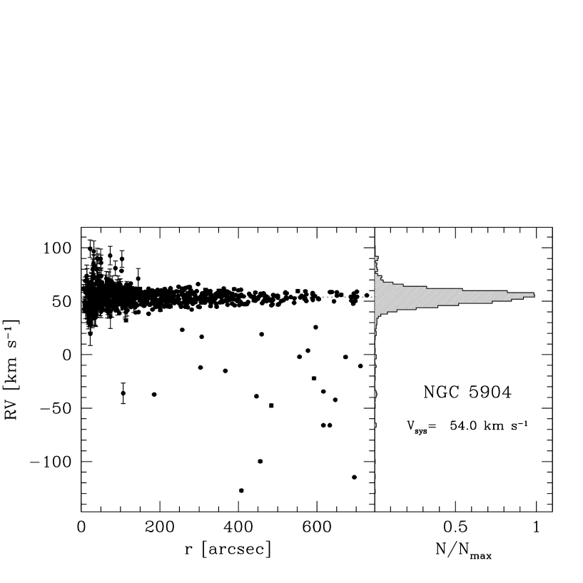
Figure 1: Left panel: Observed radial velocities as a function of the distance from the cluster center obtained in this wok. Right panel: histogram of the RV distribution, normalized to its peak value. The value of the derived systemic velocity of M5 is labelled.

The final sample of RVs in the direction of M5 consists of 857 measures for individual sources distributed out to $727\arcsec$ from the cluster center. Adopting the values quoted in Miocchi et al. (2013), this corresponds to $\sim 26$ core radii ($r_{c}=28\arcsec$) or 5 half-mass radii ($r_{h}=140\arcsec$). The innermost star is at $r=6\arcsec$, but only a dozen of measures are available within 15-$20\arcsec$ from the center because of the stellar crowding limitations. The distribution of RVs as a function of the distance from the center is plotted in Figure 1. The population of cluster members is clearly distinguishable as a narrow and strongly peaked distribution, while the Galactic field component is negligible at all radii. Assuming that the RV distribution is Gaussian, we used a Maximum-Likelihood approach (e.g., Walker et al., 2006) to estimate cluster systemic velocity and its uncertainty. For this purpose only the 677 RVs measured from FLAMES spectra have been used, and obvious outliers (as field stars) have been excluded from the analysis by means of a $3\sigma$-clipping procedure. The resulting value of the cluster systemic velocity is $V_{\rm sys}=54.0\pm 0.2$ km s^-1, in good agreement with previous determinations (see Harris 1996; Kimmig et al. 2015). In the following, we will use $V_{r}$ to indicate RVs referred to the cluster systemic velocity: $V_{r}\equiv{\rm RV}-V_{\rm sys}$.

4.2 Systemic rotation

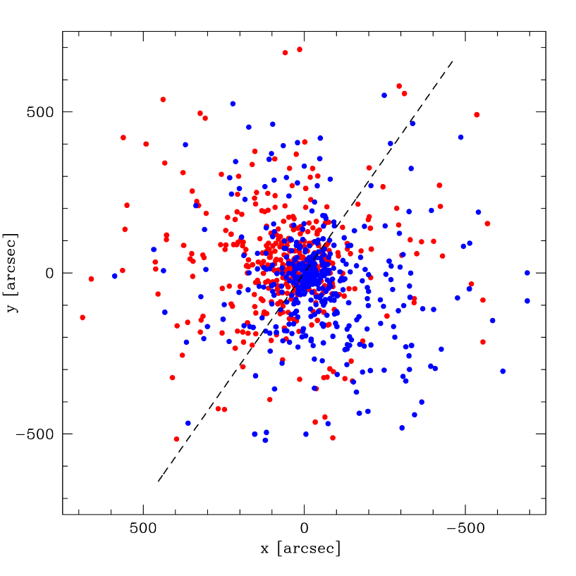
Figure 3: Distribution of the observed sample on the plane of the sky, with $x={\rm(RA-RA_{0})\cos(Dec)}$ and $y={\rm Dec-Dec_{0}}$ (RA₀ and Dec₀ being the coordinates of the cluster center, adopted from Miocchi et al., 2013). North is up, East is on the left. The colors distinguish stars with radial velocity larger than $V_{\rm sys}$ (in red), from those with $V_{r}<0$ (in blue). The dashed line marks the position of the rotation axis, which has a position angle of $145\arcdeg$ from North (as measured anti-clockwise).

A zoomed view of $V_{r}$ as a function of the distance from the center (Figure 2) clearly shows that at the outermost sampled radii (corresponding to 5 $r_{h}$) the distribution remains broad about the cluster systemic velocity. This is not expected for an isotropic pressure-supported system, where the velocity dispersion formally decreases to zero in the outskirts. It can be explained, instead, as an effect of systemic rotation. Figure 3 shows the distribution of the surveyed stars on the plane of the sky (where $x$ and $y$ are the RA and Dec coordinates referred to those of the cluster center, adopted from Miocchi et al., 2013), with the red and the blue colors indicating, respectively, positive and negative values of $V_{r}$ (i.e., RVs larger and smaller than the systemic velocity, respectively). As apparent from the figure, the evident prevalence of stars with positive values of $V_{r}$ in the upper-left portion of the map, and that of sources with $V_{r}<0$ in the lower-right part of the diagram is clear-cut signature of systemic rotation.

To investigate the rotation properties in this cluster we used the same approach adopted in Ferraro et al. (2018a) and described, e.g., in Bellazzini et al. (2012, see also , ). The method consists in splitting the RV dataset in two sub-samples with a line passing through the cluster center, and determining the difference between the mean velocity of the two groups ($\Delta V_{\rm mean}$). This is done by varying the position angle (PA) of the splitting line from $0\arcdeg$ (North direction) to $180\arcdeg$ (South direction), by steps of $10\arcdeg$, and with $90\arcdeg$ direction corresponding to the East. In the presence of rotation, $\Delta V_{\rm mean}$ draws a coherent sinusoidal variation as a function of PA, its maximum absolute value providing twice the rotation amplitude ($A_{\rm rot}$) and the position angle of the rotation axis (PA₀). The rotation of the standard coordinate system with respect to the cluster center ($x,y$) over the position angle PA₀ provides the rotated coordinate system (XR,YR), with XR set along the cluster major axis and YR aligned with the rotation axis. In a diagram showing $V_{r}$ as a function of the projected distances from the rotation axis (XR) the stellar distribution shows an asymmetry, with two diagonally opposite quadrants being more populated than the remaining two. Moreover, the sub-samples of stars on each side of the rotation axis (i.e., with positive and with negative values of XR) have different cumulative $V_{r}$ distributions and different mean velocities. To quantify the statistical significance of such differences we used three estimators: the probability that the RV distributions of the two sub-samples are extracted from the same parent family is evaluated by means of a Kolmogorov-Smirnov test, while the statistical significance of the difference between the two sample means is estimated with both the Student’s t-test and a Maximum-Likelihood approach.

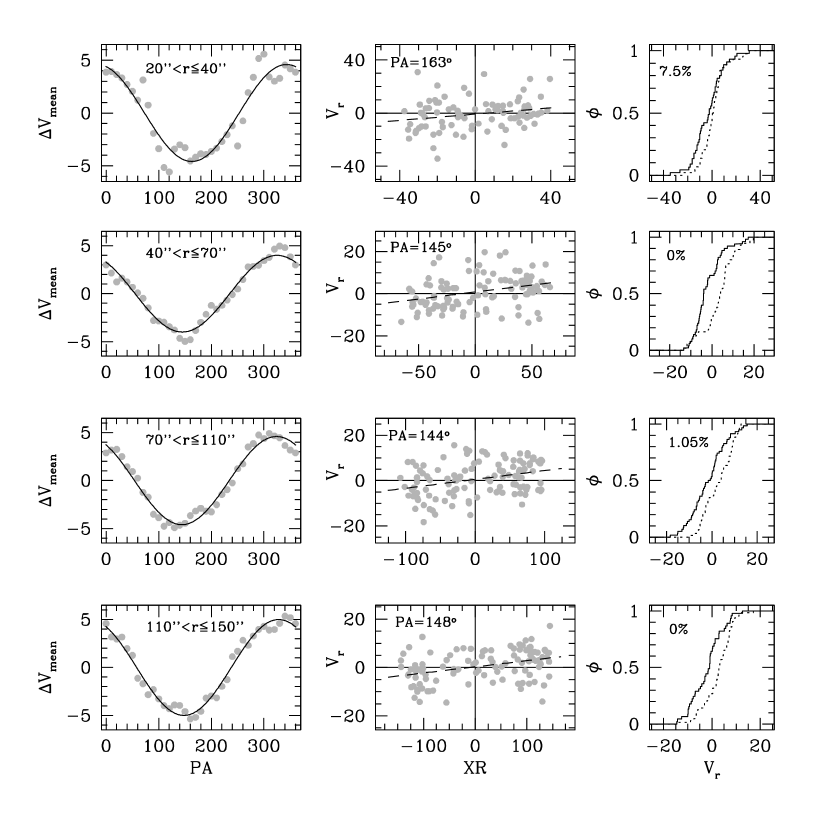
Figure 4: Diagnostic diagrams of the rotation signature detected in the first four concentric annuli listed in Table 2 (see labels in the left-hand panels). For each bin the left panel shows the difference between the mean RV on each side of a line passing through the center with a given position angle (PA), as a function of PA itself. The continuos line is the sine function that best fits the observed pattern. The central panel shows the distribution of the radial velocities $V_{r}$ as a function of the projected distances from the rotation axis (XR) in arcseconds. The position angle of the rotation axis is labelled. The dashed line is the least square fit to the data. The right panel shows the cumulative RV distributions for the sample of stars with XR$<0$ (solid line) and for that with XR$>0$ (dotted line). The Kolmogorov-Smirnov probability that the two samples on each side of the rotation axis are drawn from the same parent distribution is labelled.

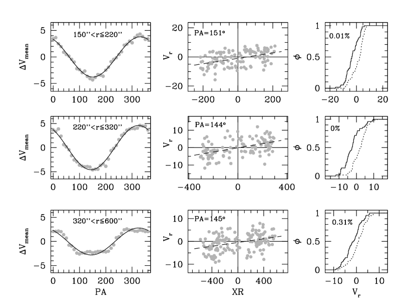
Figure 5: As in Fig. 4, but for the three outermost considered annuli (see the labels in the left-hand panels).

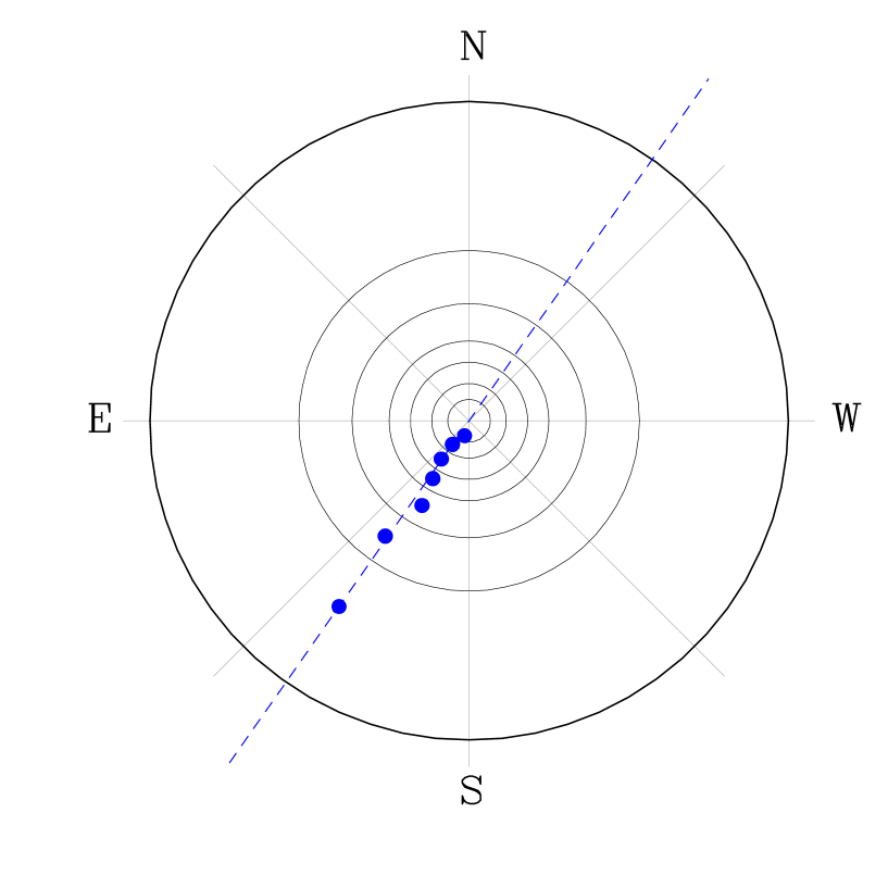
Figure 6: Position angle of the rotation axis in the radial bins listed in Table 2, used to search for rotation signatures (blue circles). As apparent, the value of PA is constant in all bins. The dashed line marks the direction of the adopted rotation axis of M5 (with position angle of $145\arcdeg$, as measured anti-clockwise from North to South).

We applied this procedure to our RV sample in a set of concentric annuli around the cluster center, avoiding the innermost region ($r<20\arcsec$), where the statistic is poor, and the outermost region ($r>600\arcsec$), where the sampling is scant and non-symmetric. The results are listed in Table 2 and plotted in Figures 4 and 5. In all the considered annuli, we find well-defined sinusoidal behaviors of $\Delta V_{\rm mean}$ as a function of PA (left-hand panels in Figs. 4 and 5), asymmetric distributions of $V_{r}$ as a function of the projected distance from the rotation axis XR (central panels), and well-separated cumulative $V_{r}$ distributions for the two samples on either side of the rotation axis (right-hand panels). The reliability of these systemic rotation signatures is also confirmed by the values of the Kolmogorov-Smirnov and t-Student probabilities and by the significance level of different sample means obtained from the Maximum-Likelihood approach (see the thee last columns in Table 2). Furthermore, as also shown in Figure 6, the position angle of the rotation axis (PA₀) is essentially constant in all the investigated annuli, as expected in the case of a coherent global rotation of the system. To conservatively determine the best-fit position angle PA₀ of the global rotation of M5 we considered only the radial range ($r>40\arcsec$) where statistically significant signatures are detected. We thus found PA${}_{0}=145\arcdeg$. Its location in the plane of the sky ($x,y$) is shown as a dashed line in Figures 3 and 6. By fixing PA₀ to this value and using all the observed stars, we finally obtain the diagnostic plots shown in Figure 7 and the values listed in Table 3 for the global rotation signatures of M5. This is one of the strongest and cleanest evidence of rotation found to date in a GC.

4.3 Ellipticity

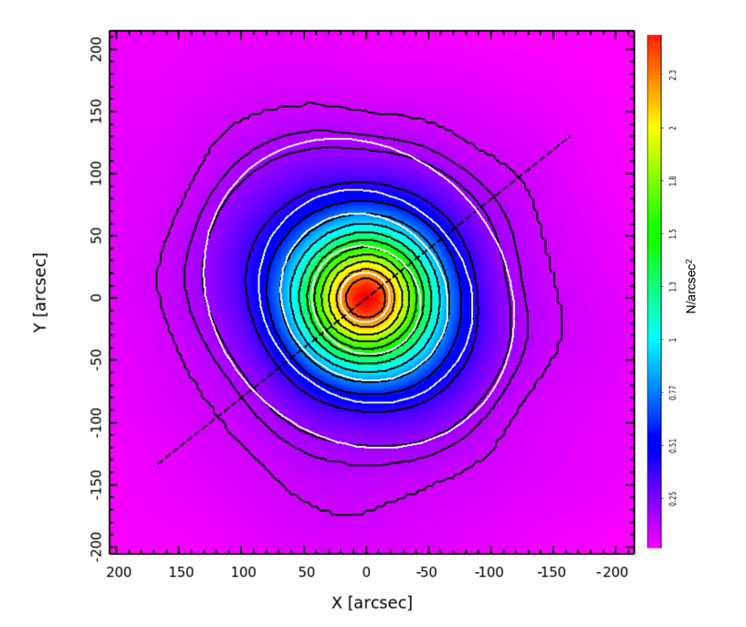
Figure 8: Stellar density map (number of stars per square arcsecond: see the color-bar) of the inner $200\arcsec\times 200\arcsec$ of M5, obtained from HST/ACS and ESO-WFI photometry. The solid black lines are isodensity contours, the white curves are their best-fit ellipses. The black dashed line marks the direction of the global rotation axis (with position angle of $145\arcdeg$).

A rapidly rotating system also is expected to be flattened in the direction perpendicular to the rotation axis (Chandrasekhar, 1969). To investigate this issue we used the HST/ACS and ESO-WFI catalogs discussed above and build the stellar density map of the system. Only stars with $V<19$ ($\sim 0.5$ magnitudes below the main sequence turn-off point) have been used to avoid incompleteness effects. This allowed us to extend the analysis out to $\sim 200\arcsec$. The resulting map is shown in Figure 8, where the black solid lines draw the isodensity contours, the white lines correspond to their best-fit ellipses and the dashed straight line marks the position of the rotation axis.

As apparent, the stellar density distribution has spherical symmetry in the center and becomes increasingly flattened in the direction perpendicular to the rotation axis for increasing radius. This trend is qualitatively consistent with that predicted, for example, by the models introduced by Varri & Bertin (2012) and found in the observational study of 47 Tucanae (Bianchini et al., 2013; Bellini et al., 2017). For the two outermost ellipses shown in the figure (at $r\sim 80\arcsec$ and $r\sim 120\arcsec$) we measure $1-b/a=0.1$ and 0.15, where $a$ and $b$ are the major and the minor axes, respectively.

4.4 Rotation curve and velocity dispersion profile

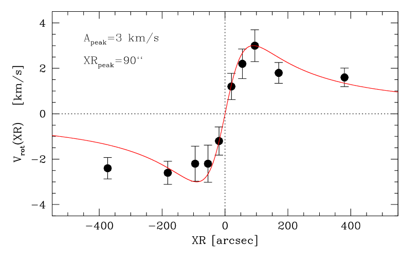
Figure 9: Rotation curve of M5. The black circles mark the stellar mean velocity as a function of the projected distance on either side of the rotation axis (XR) for the intervals listed in Table 4. The red line, which well reproduces the observed curve, has the functional form expressed in equation (1), with $A_{\rm peak}=3$ km s^-1 and ${\rm XR_{peak}}=90\arcsec$.

To determine the rotation curve of M5 we considered the rotated coordinate system (XR,YR) and split the $V_{r}$ sample in five intervals of XR on both sides of the rotation axis. We then used the Maximum-Likelihood method described in Walker et al. (2006, see also Martin et al. 2007; Sollima et al. 2009) to determine the mean velocity of all the stars belonging to each XR bin. The errors have been estimated following Pryor & Meylan (1993). The resulting rotation curve (Figure 9 and Table 4) clearly shows the expected shape, with an increasing trend in the innermost regions up to a maximum value, and a decreasing behavior outward. The analytic expression (Lynden-Bell, 1967) appropriate for cylindrical rotation:

$$V_{\rm rot}=\frac{2A_{\rm peak}}{\rm XR_{peak}}~{}~{}\frac{\rm XR}{1+({\rm XR}/{\rm XR_{peak}})^{2}}$$ (1)

very well reproduces the observed rotation curve (see the red solid line in Figure 9), with a maximum amplitude of $\sim 3$ km s^-1 at $\sim 90\arcsec$ from the rotation axis.

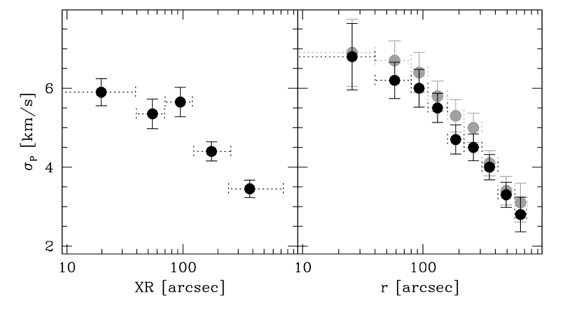
Figure 10: Velocity dispersion profile of M5 obtained in two different projections. Left-hand panel: folded velocity dispersion profile determined in the same shells of projected distance from the rotation axis (XR) used for the rotation curve plotted in Fig. 9. The corresponding values and error bars are listed in the last two columns of Table 4. Right-hand panel: velocity dispersion profile obtained in concentric circular annuli around the cluster center (solid circles; see also Table 5). For sake of illustration, we also show the profile of the second velocity moment, which includes the effects of both rotation and velocity dispersion in each circular shell (grey circles and last two columns in Table 5).

By folding the two RV samples on either side of the rotation axis and using the same five intervals of XR adopted for the rotation curve, we obtained the projected velocity dispersion profile shown in the left-hand panel of Figure 10 and listed in the last two columns of Table 4. We emphasize that the velocity dispersion profiles most commonly shown in the literature are determined in circular annuli around the cluster center, rather than in shells of projected radial distances from the rotation axis (XR), as done in this figure. However, in the presence of a clear global rotation of the system, it is reasonable to assume cylindrical symmetry and thus to show the kinematical properties in the rotated coordinate system (XR,YR). Indeed, this allows a direct comparison with the rotation velocity (Fig. 9), which is determined in the same projection. This comparison clearly shows that, in spite of a clean and relatively strong rotation, M5 is still dominated by non-ordered motions at all distances from the rotation axis: in fact, the velocity dispersion is larger than the rotation velocity in all the considered bins.

The projected velocity dispersion profile of M5 obtained in circular concentric shells is shown in the right-hand panel of Figure 10 (black circles) and listed in Table 5. This has been determined after subtracting from the measured RV of each star, the mean velocity of the XR shell to which the star belongs. For sake of illustration we also show the radial profile of second velocity moment (grey circles), i.e., the dispersion of the RVs measured within each circular bin, with no subtraction of the rotational component. Of course, the velocity dispersion is smaller than the second velocity moment in every bin. However, the differences are small and always within the errors, as expected in the case of a pressure-supported system. The comparison between the left-hand panel and the right-hand panel (black circles) of Fig. 10 clearly shows that the central values of the velocity dispersion obtained by using XR shells are smaller than those determined in circular annuli. This is due to the fact that, by construction, the inner XR shells include stars that are spatially close to the rotation axis, but orbit both in the cluster central regions (hence, with large velocity dispersion) and at the cluster periphery (hence, with small velocity dispersion). The innermost circular annulus, instead, is largely dominated by stars that are truly orbiting close to the center, and the “dilution” effect due to physically distant stars is much smaller.

Since our observations extend out $\sim 10\arcmin$ away from the center, the projection of the cluster space motion along the line-of-sight could produce a non-negligible amount of apparent rotation. To estimate the contribution of such perspective rotation to the true rotational velocity of M5 we followed the procedure described in van de Ven et al. (2006), adopting the values quoted in Narloch et al. (2017) for the systemic proper motion of M5. We found a mild variation of the position angle of the rotation axis (PA${}_{0}=141\arcdeg$, instead of $145\arcdeg$) and values of $V_{\rm rot}$ and $\sigma_{P}$ in very good agreement (well within the errors) with those quoted in Table 4. These results and the fact that updated values of the cluster proper motion will become available soon (thanks to the upcoming Gaia second data release), we decide not to apply perspective rotation corrections to our determinations.

5 Discussion

As part of the ESO-VLT MIKiS Survey (Ferraro et al., 2018a), we presented solid and unambiguous evidence of strong global rotation between $\sim 0.5r_{h}$ and $5r_{h}$ in the Galactic globular cluster M5. Signatures of systemic rotation in this system, both in the outskirts and in the central regions, were already presented in previous works. Bellazzini et al. (2012) found a rotation signal, with an amplitude of 2.6 km s^-1 and a position angle of $157\arcdeg$, from the analysis of 136 individual star spectra at $\sim 60\arcsec<r<600\arcsec$. From a sample of 128 stars distributed between $\sim 70\arcsec$ and $\sim 1400\arcsec$, Kimmig et al. (2015) report an amplitude of 2.1 km s^-1. Fabricius et al. (2014) performed an integrated-light spectroscopic study of the innermost $\sim 60\arcsec\times 60\arcsec$ of M5, finding a central velocity gradient of 2.1 km s^-1 and a position angle of the rotation axis of $148.5\arcdeg$ (once reported in the coordinate system adopted here). Very recently, Kamann et al. (2018) analyzed a large number of individual star spectra acquired at $r<60\arcsec$ with the integral-field spectrograph ESO-MUSE, and found a velocity gradient of 2.2 km s^-1. They measured the rotation axis position angle in different radial bins around the cluster center, finding PA${}_{0}\sim 130\arcdeg-140\arcdeg$ (once reported in our system) at $r>10\arcsec$, while the axis seems to be rotated by $90\arcdeg$ in the innermost region. Although a detailed comparison of the rotation amplitude among the various works is not straightforward (because of the different radial regions sampled and/or the different parameters adopted to quantify it), typical values of $\sim 2$ km s^-1 are found in all the studies. A very good agreement is also found for what concerns the position angle of the rotation axis. The only exception is the perpendicular direction found by Kamann et al. (2018) in the innermost $10\arcsec$ of the cluster. Higher spatial-resolution spectroscopy, with the enhanced version of MUSE (WFM-AO, which operates under super-seeing conditions down to FWHM$\sim 0.4\arcsec$), or with the adaptive-optics corrected spectrograph ESO-SINFONI (see Lanzoni et al., 2013), will shed new light on this intriguing feature.

With respect to previous works, our study has the advantage of being based on a much larger statistics at $r>60\arcsec$. Hence, with the exception of the central region, it provides the most solid and precise determination of the rotation axis, rotation curve and velocity dispersion profile of M5. Indeed, Fig. 6 probably shows the cleanest evidence so far of a constant value of PA₀ with radius, testifying a coherent rotation and a reliable determination of the central kinematics of this cluster. The resulting rotation curve is illustrated in Fig. 9. This profile is well reproduced by the analytic expression presented in equation (1), which is appropriate for cylindrical rotation and is inspired by the structure of the velocity space of stellar systems resulting from the process of violent relaxation (Lynden-Bell, 1967; Gott, 1973). The observed peak rotation amplitude is $A_{\rm peak}\sim 3$ km s^-1 and is located at about $0.6r_{h}$ from the center. The radial distribution of the angular momentum is such that the behavior in the central regions is consistent with solid-body rotation, while in the outer portion of the radial range under consideration, it declines smoothly. Of course, kinematic information along the line of sight provides exclusively a lower limit to the three-dimensional rotation content, due to projection effects.

To study the relative importance of ordered versus random motions and to quantify the role of rotation in shaping the geometry of a stellar system, the ratio between the peak rotational velocity and the central velocity dispersion is commonly used (for recent studies, see, e.g., Bianchini et al., 2013; Kacharov et al., 2014; Jeffreson et al., 2017). Since our data do not sample the inner region of M5, we adopt the central velocity dispersion $\sigma_{0}=7.3$ km s^-1 quoted by Kamann et al. (2018), finding $V_{\rm peak}/\sigma_{0}=0.4$. As discussed in Sect. 4.3, we adopt $e=0.15$ for the cluster ellipticity. In a plot of $V_{\rm peak}/\sigma_{0}$ versus the ellipticity, M5 is the GC with largest rotational support that exactly locates on the line of isotropic oblate rotators viewed edge-on (see, e.g., Figure 14 in Bianchini et al., 2013). Hence, on the basis of this simple argument, we suggest that the observed rotation amplitude is likely close to the three-dimensional one (i.e., the stellar system is observed on a line-of-sight which is close to the edge-on projection), and the flattening of this cluster could be explained by its own internal rotation.

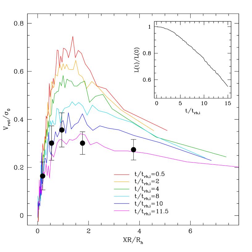
Figure 11: Time evolution of the radial profile of $V_{\rm rot}/\sigma_{0}$ from one of the N-body simulations of Tiongco et al. (2016, the VBrotF04 model, see their Table 1). The radial distances from the rotation axis (XR) are express in units of the projected half-mass radius ($R_{h}=100\arcsec$; from Miocchi et al., 2013). An inclination angle between the line-of-sight and the rotation axis of $20\arcdeg$ is assumed in the calculation of the radial profiles. Each line shows the radial profile of $V_{\rm rot}/\sigma_{0}$ calculated at different times (see labels, where $t_{\rm rh,i}$ is the cluster’s initial half-mass relaxation time). Each profile is calculated by combining three snapshots around the desired time. The black filled circles show the observed radial profile of M5: each point is the average of the $V_{\rm rot}$ values determined on the two sides of the rotation axis (see Table 4), normalized to the central velocity dispersion from Kamann et al. (2018). The inset shows the time evolution of the cluster’s total angular momentum (L), normalized to its initial value.

In a forthcoming article, we will present a complete investigation based on a global, self-consistent, axisymmetric dynamical model, characterized by differential rotation and anisotropy in the velocity space (e.g. Varri & Bertin, 2012), coupled with appropriate N-body simulations (e.g. Tiongco et al., 2016, 2017, 2018). Nonetheless, here we present a first comparison between the radial profile of the ratio $V_{\rm rot}/\sigma_{0}$ and the time evolution of such a kinematic observable, as resulting from a representative N-body model from the survey recently conducted by Tiongco et al. (2016, 2018). Such a comparison, which is illustrated in Figure 11, supports the conclusion that M5 has already experienced the effects of two-body relaxation and angular momentum transport over the course of several initial half-mass relaxation times ($t_{\rm rh,i}$). This simple analysis should be intended only as a proof-of-concept that, in most cases, the angular momentum measured in present-day GCs represent a lower limit of the amount they possessed at birth (for the time evolution of the total angular momentum of the model, see the figure inset). We wish to emphasize that this comparison did not require any ad-hoc tailoring of the initial conditions of the N-body model, and involved exclusively a simple exploration of the projected observables over different lines-of-sight. The inclination angle adopted in the figure ($20\arcdeg$) is in qualitative agreement with the conclusion of an nearly edge-on view of the system discussed above. However, this value should be considered only as a representative example of a range of acceptable values, while a definitive assessment requires a full investigation of the degeneracy between intrinsic rotation and projection effects, which will be presented in the forthcoming dynamical study.

Rotation patterns as clear as those found in M5 have been detected just in a few other cases so far (see the cases of NGC 4372 in Kacharov et al. 2014, and 47 Tucanae in Bellini et al. 2017). However, evidence of systemic rotation signatures is mounting, with the most recent results for 9 GCs presented in Ferraro et al. (2018a, but see also , and references therein). This suggests that possibly most (if not all) Galactic GCs are characterized by some degree of internal rotation, that migh be the residual of a much larger amount of ordered motions imprinted at birth and gradually dissipated via angular momentum transport (due to two-body relaxation) and mass loss (e.g., Fiestas et al., 2006; Tiongco et al., 2017, see also Fig. 11). Then, once combined with independent measures of the level of dynamical evolution determined, e.g., from the radial distribution of blue straggler stars (see Ferraro et al., 2009, 2012, 2018b; Lanzoni et al., 2016; Raso et al., 2017), these signals may be used to clarify the formation and evolutionary histories of GCs, and the relative role of rotation. This outlook substantiates the urgency of multi-spectrograph studies of Galactic GCs (as the MIKiS Survey), sensible enough to detect even weak rotation signals in these systems. It also motivates the investment of renewed energies in the theoretical investigation of the role of angular momentum in collisional stellar dynamics, with appropriate equilibrium and evolutionary dynamical models.

Program ID	Grating	PI
193.D-0232	HR21	(Ferraro)
073.D-0695	HR5	(Recio Blanco)
088.B-0403	HR9	(Lucatello)
073.D-0211	HR11	(Carretta)
087.D-0230	HR12	(Gratton)
073.D-0211	HR13	(Carretta)
087.D-0276	HR15	(D’Orazi)

Table 1: Summary of the FLAMES datasets used to derive the internal kinematics of M5. The MIKiS Survey sample corresponds to Program ID 193.D-0232, while the others have been retrieved from the ESO archive.

$r_{i}$	$r_{e}$	$r_{m}$	$N$	PA0	$A_{\rm rot}$	$P_{\rm KS}$	$P_{\rm Stud}$	n-$\sigma_{\rm ML}$
20	40	29.4	89	163	2.3	$7.5\times 10^{-2}$	$>90.0$	1.4
40	70	54.0	105	145	2.0	$1.0\times 10^{-5}$	$>99.8$	4.2
70	110	88.8	118	144	2.3	$1.1\times 10^{-2}$	$>99.8$	3.4
110	150	128.3	108	148	2.5	$5.0\times 10^{-5}$	$>99.8$	3.9
150	220	182.0	111	151	1.9	$1.5\times 10^{-4}$	$>99.8$	4.8
220	320	268.0	107	144	2.3	$1.0\times 10^{-5}$	$>99.8$	4.7
320	600	426.2	141	145	1.4	$3.1\times 10^{-3}$	$>99.8$	3.6

Table 2: Rotation signatures detected in circular annuli around the cluster center. For each annulus the table lists: the inner and outer radius ($r_{i}$ and $r_{e}$) in arcseconds, the mean radius and the number of stars in the bin ($r_{m}$ and $N$, respectively), the position angle of the rotation axis (PA₀), the rotation amplitude (A_rot), the Kolmogorov-Smirnov probability that the two samples on each side of the rotation axis are drawn from the same parent distribution ($P_{\rm KS}$), the t-Student probability that the two RV samples have different means ($P_{\rm Stud}$), and the significance level (in units of n-$\sigma$) that the two means are different following a Maximum-Likelihood approach (n-$\sigma_{\rm ML}$).

$r_{i}$	$r_{e}$	$r_{m}$	$N$	PA0	$A_{\rm rot}$	$P_{\rm KS}$	$P_{\rm Stud}$	n-$\sigma_{\rm ML}$
6	727	186.3	823	145	2.0	$1.0\times 10^{-17}$	$>99.8$	9.9

Table 3: The same as in Table 2, but for the entire radial range ($6\arcsec-727\arcsec$) covered by the observations and after fixing the position angle of the rotation axis to PA${}_{0}=145\arcdeg$.

XRi	XRe	XR${}_{m}+$	$N+$	$V_{\rm rot}+$	$\epsilon_{V+}$	XR${}_{m}-$	$N-$	$V_{\rm rot}-$	$\epsilon_{V-}$	$\sigma_{P}$(XR)	$\epsilon_{\sigma_{P}}$
0	40	20.2	131	1.2	0.6	-19.3	134	-1.2	0.6	5.9	0.3
40	70	55.0	69	2.2	0.6	-54.3	55	-2.2	0.8	5.4	0.4
70	120	94.6	64	3.0	0.7	-95.2	65	-2.2	0.8	5.6	0.4
120	250	170.6	91	1.8	0.5	-182.1	79	-2.6	0.5	4.4	0.2
250	727	379.9	65	1.6	0.4	-373.3	65	-2.4	0.5	3.4	0.2

Table 4: Rotation curve and folded velocity dispersion profile of M5 in the rotated system (XR,YR). For five intervals of projected distances from the rotation axis (XR), the tables lists: the inner and outer absolute limits of each bin (XR_i and XR_e) in arcseconds, the mean distance, number of stars, average velocity and its error (in km s^-1) on the positive side of the XR axis (columns 3–6), the same for the negative side of the XR axis (columns 7–10), and the folded velocity dispersion and its error (columns 11-12).

$r_{i}$	$r_{e}$	$r_{m}$	$N$	$\sigma_{P}(r)$	$\epsilon_{\sigma}$	$\tilde{\sigma}_{P}(r)$	$\epsilon_{\tilde{\sigma}}$
6	40	25.8	116	6.8	0.8	6.9	0.9
40	80	58.2	132	6.2	0.5	6.7	0.5
80	110	93.0	91	6.0	0.5	6.4	0.5
110	160	132.2	126	5.5	0.4	5.8	0.4
160	220	187.2	93	4.7	0.4	5.3	0.4
220	310	262.5	96	4.5	0.3	5.0	0.4
310	420	357.6	88	4.0	0.3	4.1	0.3
420	580	492.5	58	3.3	0.3	3.4	0.4
580	727	648.3	23	2.8	0.4	3.1	0.5

Table 5: Velocity dispersion and second velocity moment profiles of M5 determined in circular annuli around the cluster center: internal and external radius of each annulus in arcseconds (columns 1,2), average cluster-centric distance and number of stars in the bin (columns 3,4), projected velocity dispersion (km s^-1) and its uncertainty (columns 5,6), projected second velocity moment and its uncertainty (columns 7,8).

Figure 2: Left panel: Zoomed view of the radial distribution of the measured velocities referred to $V_{\rm sys}$. The large scatter observable at large distances from the cluster center is a clear signature of systemic rotation. The two arrows indicate the projected half-light (or, equivalently, half-mass) radius and the three-dimensional half-mass radius of M5 ($R_{h}=100\arcsec$ and $r_{h}=140\arcsec$, respectively; from Miocchi et al., 2013).

Figure 7: Diagnostic diagrams of the global rotation of M5. The meaning of each panel is as in Figs. 4 and 5, but here we plot all the observed stars (with cluster-centric distances $6\arcsec<r\leq 727\arcsec$), assuming PA${}_{0}=145\arcdeg$ as position angle of the rotation axis.

References

- Anderson & King (2003) Anderson, J., & King, I. R. 2003, AJ, 126, 772
- Bellazzini et al. (2012) Bellazzini, M., Bragaglia, A., Carretta, E., et al. 2012, A&A, 538, A18
- Bellazzini et al. (2015) Bellazzini, M., Mucciarelli, A., Sollima, A., et al. 2015, MNRAS, 446, 3130
- Bellini et al. (2014) Bellini, A., Anderson, J., van der Marel, R. P., et al. 2014, ApJ, 797, 115
- Bellini et al. (2017) Bellini, A., Bianchini, P., Varri, A. L., et al. 2017, ApJ, 844, 167
- Bianchini et al. (2013) Bianchini, P., Varri, A. L., Bertin, G., & Zocchi, A. 2013, ApJ, 772, 67
- Bianchini et al. (2016) Bianchini, P., van de Ven, G., Norris, M. A., Schinnerer, E., & Varri, A. L. 2016, MNRAS, 458, 3644
- Boberg et al. (2017) Boberg, O. M., Vesperini, E., Friel, E. D., Tiongco, M. A., & Varri, A. L. 2017, ApJ, 841, 114
- Carballo-Bello et al. (2018) Carballo-Bello, J. A., Martínez-Delgado, D., Navarrete, C., et al. 2018, MNRAS, 474, 683
- Chandrasekhar (1969) Chandrasekhar, S. 1969, The Silliman Foundation Lectures, New Haven: Yale University Press, 1969,
- Chen & Chen (2010) Chen, C. W., & Chen, W. P. 2010, ApJ, 721, 1790
- Cordero et al. (2017) Cordero, M. J., Hénault-Brunet, V., Pilachowski, C. A., et al. 2017, MNRAS, 465, 3515
- Correnti et al. (2011) Correnti, M., Bellazzini, M., Dalessandro, E., et al. 2011, MNRAS, 417, 2411
- Fabricius et al. (2014) Fabricius M. H. et al., 2014, ApJ, 787, L26
- Ferraro et al. (2009) Ferraro, F. R., Beccari, G., Dalessandro, E., et al. 2009, Nature, 462, 1028
- Ferraro et al. (2012) Ferraro, F. R., Lanzoni, B., Dalessandro, E., et al. 2012, Nature, 492, 393
- Ferraro et al. (2018a) Ferraro, F. R., Mucciarelli, A., Lanzoni, B., et al. 2018a, ApJ, in press (arXiv:1804.08618)
- Ferraro et al. (2018b) Ferraro, F. R., Lanzoni, B., Raso, S., et al. 2018b, ApJ, in press
- Fiestas et al. (2006) Fiestas, J., Spurzem, R., & Kim, E. 2006, MNRAS, 373, 677
- Gott (1973) Gott, R. J., III 1973, ApJ, 186, 481
- Harris (1996) Harris, W. E. 1996, AJ, 112, 1487, 2010 edition
- Jeffreson et al. (2017) Jeffreson, S. M. R., Sanders, J. L., Evans, N. W., et al. 2017, MNRAS, 469, 4740
- Kacharov et al. (2014) Kacharov, N., Bianchini, P., Koch, A., et al. 2014, A&A, 567, A69
- Kamann et al. (2018) Kamann, S., Husser, T.-O., Dreizler, S., et al. 2018, MNRAS, 473, 5591
- Kimmig et al. (2015) Kimmig, B., Seth, A., Ivans, I. I., et al. 2015, AJ, 149, 53
- King (1966) King I.R., 1966, AJ, 71, 64
- Lane et al. (2009) Lane, R. R., Kiss, L. L., Lewis, G. F., et al. 2009, MNRAS, 400, 917
- Lane et al. (2010) Lane, R. R., Kiss, L. L., Lewis, G. F., et al. 2010, MNRAS, 406, 2732
- Lanzoni et al. (2007a) Lanzoni, B., Dalessandro, E., Ferraro, F. R., et al. 2007, ApJ, 663, 267
- Lanzoni et al. (2013) Lanzoni, B., Mucciarelli, A., Origlia, L., et al. 2013, ApJ, 769, 107
- Lanzoni et al. (2016) Lanzoni, B., Ferraro, F. R., Alessandrini, E., et al. 2016, ApJ, 833, L29
- Lardo et al. (2015) Lardo, C., Pancino, E., Bellazzini, M., et al. 2015, A&A, 573, A115
- Lynden-Bell (1967) Lynden-Bell, D. 1967, MNRAS, 136, 101
- Marino et al. (2014) Marino, A. F., Milone, A. P., Yong, D., et al. 2014, MNRAS, 442, 3044
- Martin et al. (2007) Martin, N. F., Ibata, R. A., Chapman, S. C., Irwin, M., & Lewis, G. F. 2007, MNRAS, 380, 281
- McLaughlin & van der Marel (2005) McLaughlin, D. E., & van der Marel, R. P. 2005, ApJS, 161, 304
- Miocchi et al. (2013) Miocchi, P., Lanzoni, B., Ferraro, F. R., et al. 2013, ApJ, 774, 151
- Narloch et al. (2017) Narloch, W., Kaluzny, J., Poleski, R., et al. 2017, MNRAS, 471, 1446
- Olszewski et al. (2009) Olszewski, E. W., Saha, A., Knezek, P., et al. 2009, AJ, 138, 1570
- Pasquini et al. (2000) Pasquini, L., Avila, G., Allaert, E., et al. 2000, Proc. SPIE, 4008, 129
- Pryor & Meylan (1993) Pryor, C., & Meylan, G. 1993, Structure and Dynamics of Globular Clusters, 50, 357
- Raso et al. (2017) Raso, S., Ferraro, F. R., Dalessandro, E., et al. 2017, ApJ, 839, 64
- Sarajedini et al. (2007) Sarajedini, A., Bedin, L. R., Chaboyer, B., et al. 2007, AJ, 133, 1658
- Sbordone et al. (2004) Sbordone, L., Bonifacio, P., Castelli, F., & Kurucz, R. L., MSAIS, 5, 93
- Sharples et al. (2010) Sharples, R., Bender, R., Agudo Berbel, A., et al. 2010, The Messenger, 139, 24
- Sollima et al. (2009) Sollima, A., Bellazzini, M., Smart, R. L., et al. 2009, MNRAS, 396, 2183
- Tiongco et al. (2016) Tiongco, M. A., Vesperini, E., & Varri, A. L. 2016, MNRAS, 461, 402
- Tiongco et al. (2017) Tiongco, M. A., Vesperini, E., & Varri, A. L. 2017, MNRAS, 469, 683
- Tiongco et al. (2018) Tiongco, M. A., Vesperini, E., & Varri, A. L. 2018, MNRAS, 475, L86 E., & Varri, A. L. 2018, MNRAS, (in press)
- Tonry & Davis (1979) Tonry, J. & Davis, M., 1979, AJ, 84, 1511
- Trenti & van der Marel (2013) Trenti, M., & van der Marel, R. 2013, MNRAS, 435, 3272
- van de Ven et al. (2006) van de Ven, G., van den Bosch, R. C. E., Verolme, E. K., & de Zeeuw, P. T. 2006, A&A, 445, 513
- Varri & Bertin (2012) Varri, A. L., & Bertin, G. 2012, A&A, 540, A94
- Vesperini et al. (2014) Vesperini, E., Varri, A. L., McMillan, S. L. W., & Zepf, S. E. 2014, MNRAS, 443, L79
- Walker et al. (2006) Walker, M. G., Mateo, M., Olszewski, E. W., et al. 2006, AJ, 131, 2114
- Watkins et al. (2015) Watkins, L. L., van der Marel, R. P., Bellini, A., & Anderson, J. 2015, ApJ, 803, 29