Simulation model for the propagation of second mode streamers in dielectric liquids using the Townsend–Meek criterion

Abstract

A simulation model for second mode positive streamers in dielectric liquids is presented. Initiation and propagation is modeled by an electron-avalanche mechanism and the Townsend–Meek criterion. The electric breakdown is simulated in a point-plane gap, using cyclohexane as a model liquid. Electrons move in a Laplacian electric field arising from the electrodes and streamer structure, and turn into electron avalanches in high-field regions. The Townsend–Meek criterion determines when an avalanche is regarded as a part of the streamer structure. The results show that an avalanche-driven breakdown is possible, however, the inception voltage is relatively high. Parameter variations are included to investigate how the parameter values affect the model.

Keywords: Simulation model, Streamer, Electron avalanche, Townsend–Meek criterion, Dielectric liquid, Electrical breakdown

1 Introduction to streamers

Dielectric liquids are widely used for insulation of high power equipment, such as transformers, since liquid insulation has good cooling properties, high electrical withstand strength, and recovers from an electrical discharge within short time [1]. Electric breakdown in liquids is preceded by the formation of a prebreakdown channel called a streamer [2]. A partial discharge, a local electric breakdown, changes the electric field distribution, which could cause another local breakdown, and in this way, a streamer may propagate through a liquid. A streamer bridging the gap between two electrodes, for instance an energized part and a grounded part, lowers the electrical withstand strength and may cause a complete electric breakdown, possibly destroying the equipment [1].

A streamer consists of a gaseous and partly ionized structure, originating in one location and branching out in filaments as it propagates through the liquid. This structure may be observed through shadowgraphic or schlieren photography since its refractive index differs from the surrounding liquid [3]. Streamers are classified as positive or negative, depending on the polarity of the initiation site. Streamer experiments are often carried out in needle-plane gaps since a strongly divergent field allows control of where the streamer initiates, the polarity of the streamer, and also enables the study of streamers that initiate, propagate, and then stops without causing an electric breakdown [3, 2]. Conversely, in a gap with a uniform field, inception governs the breakdown probability, since an initiated streamer is always able to propagate the gap due to the high background field.

The nature of streamers has been investigated for decades [3, 4, 5, 6, 7, 8, 9, 10, 11, 12, 13, 14, 1, 2], but is still not well understood. For positive streamers in non-polar liquids, it is common to define four distinct modes of propagation, mainly characterized by their speed [15, 2]. The streamer mode depends on the applied voltage, and may change during propagation. The 1st mode propagates in a bubbly or bushy fashion with a speed of the order of $100\text{\,}\mathrm{m}\text{\,}{\mathrm{s}}^{-1}$, the 2nd mode is faster, of the order of $1\text{\,}\mathrm{km}\text{\,}{\mathrm{s}}^{-1}$, and has a branched or tree-like structure. The even faster 3rd and 4th modes propagates at speeds of the order of $10\text{\,}\mathrm{km}\text{\,}{\mathrm{s}}^{-1}$ and $100\text{\,}\mathrm{km}\text{\,}{\mathrm{s}}^{-1}$, respectively. The 1st mode is only observed for very sharp needles and will usually not lead to a breakdown by itself, but the streamer may change to the 2nd mode. The 2nd mode may initiate for voltages below the voltage required for breakdown, and increases in propagation length and number of branches at higher voltages. Often, a 2nd mode streamer sporadically emits visible light [3], re-illuminations, from one or more of its branches. Above the breakdown voltage, streamers may change between the 2nd, the 3rd, and the 4th mode during propagation. There are usually more re-illuminations in the 3rd mode than the 2nd mode. The inception of the 4th mode is associated with a drastic increase in speed and fewer, more luminous, branches [2].

There are numerous mechanisms that can be involved in the streamer phenomena, the challenge is identifying their importance during initiation and propagation. Applying a potential to a needle can cause charge injection, giving a space-charge limited current [16] causing Joule heating [16], which in turn can cause bubble nucleation [17]. A breakdown in the gas bubble can then propagate the needle potential, and the process may repeat. This is one way to explain 1st mode propagation. Electric fields can also cause electrohydrodynamic flow, which could cause streamer formation through cavitation [18]. Electrostatic cracking has also been proposed as a cavitation mechanism [19]. A main topic of discussion is whether a lowering of the liquid density is needed before charge generation can occur. Electron avalanches are important in gas discharge, but their importance in liquid breakdown is still disputed. In water, strong scattering could prevents electrons from forming avalanches in the liquid phase [20]. Therefore, discharges in micro-bubbles can be important for charge generation [20, 10, 14]. The same mechanism was also proposed for non-polar liquids [19], however, the relative permittivity is about 80 in water and about 2 in a typical oil, and this difference can prove important since the field enhancement within a bubble in oil is much lower than in water. Contrary to water, there are indications of electron avalanches in non-polar liquids [21, 22, 16], furthermore, while the initiation and the propagation length of 2nd mode streamers are dependent on the pressure, their propagation velocity is not pressure dependent [23, 16]. This implies that the mechanism responsible for propagation occurs in the liquid phase and that the gaseous channel follows as a consequence. In very high electric fields, field-ionization can occur [24, 25], and this mechanism has been proposed for the fast 3rd and 4th propagation modes[7]. As the streamer gains length, the properties of the channel could also prove important. The streamer channel is a partly ionized, low-temperature plasma, having a varying conductance [26, 8]. The mechanisms involved when a plasma is in contact with a liquid is often overlooked and is in itself a very complex problem [27].

The development of models is important for improving electrical equipment as well as the prevention of equipment failure. An early simulation model for liquid breakdown uses a lattice to investigate the fractal nature of the streamer structure as a function of the electric field $E$ [28], and has been expanded to incorporate needle-plane geometry [29], a 3D-lattice [30], statistical time [31], availability of seed electrons [32], and varying conductance of the streamer channels [33]. Charge generation and transport in an electric field have also been solved by a finite element method (FEM) approach, to simulate streamer propagation in 2D and 3D, adding impurities to generate streamer branching [34, 35, 36, 37]. A major difference between breakdown in gases and liquids is that a phase change is involved when making the streamer channel in liquids. The phase change is difficult to model, but it is possible to make approximations [38], or to focus on the plasma within the channel [39].

Both lattice and FEM simulations require considerable computational power, and therefore, the simulations are often done for either very short timescales or very simplified models. The work presented here is based on [40], which chooses a different approach. It is a computational model for 2nd mode positive streamers in non-polar liquids, driven by electron avalanches in the liquid phase. A point-plane geometry is modeled, with the point being a positively charged hyperbolic needle. Cyclohexane is used as a model liquid, since it is a well defined system used extensively in experiments [25, 22, 5, 41, 11].

The model and the theoretical background is presented in section 2, as well as the parameters and the algorithm used for the simulations. In section 3, the results are given and discussed. First a baseline is established, then parameter variations and alternative parameter values are investigated. A general discussion, outlining the weaknesses and strengths of the model, is given in section 4. Finally, the main conclusions are summarized in section 5. A contains additional details on the coordinate system used in the model.

2 Simulation model and theory

The model is built on the assumption that electron avalanches occur in the liquid phase, and that these govern the propagation of 2nd mode, positive streamers [40].

Applying a potential to the needle in a needle-plane geometry gives rise to an electric field. A number of anions and electrons, assumed to be already present in the liquid, are accelerated by the electric field. Subsequently, electron multiplication occurs in areas where the electric field is sufficiently strong, turning electrons into electron avalanches. An avalanche is assumed to be “critical” if it reaches a magnitude given by the Townsend–Meek criterion [42], and the position of such an avalanche is regarded as a part of the streamer. Then the electric field is reevaluated, accounting for the potential of both the needle and the streamer. This work investigates liquid cyclohexane as the insulating liquid, with the option to add dimethylaniline (DMA) as an additive, but the model can be used for other base liquids and additives as well, if the parameter values are available.

2.1 Geometrical and electrical properties

Figure 1: The hyperbolic needle and a streamer head, with relevant variables shown. The distance to the plane is usually far greater than illustrated here.

A hyperbolic needle electrode with a tip radius $r_{\textrm{p}}$ is placed at a distance $d_{\textrm{g}}$ from a planar electrode, as illustrated in figure 1 where all important geometric variables are shown. In prolate spheroid coordinates ($\mu,\nu,\phi;a$), a hyperboloid is represented by a single coordinate $\nu$, and the 3D Laplace equation becomes separable, see A for details and definitions. The potential is (cf. 49)

$$V_{i}=C_{i}\ln\tan\frac{\nu_{i}}{2}\,,$$ (1)

and the electric field is (cf. 51)

$$\bm{E}_{i}=\frac{C_{i}\,\hat{\bm{\nu}}_{i}}{h_{\nu_{i}}\sin\nu_{i}}\,,$$ (2)

where $C_{i}$ is a constant. The subscript $i$ refers to a given hyperboloid (the needle or a streamer head), hence, the subscript in $\nu_{i}$ implies a transformation to a coordinate system centered at hyperboloid $i$,

$$\nu_{i}(\bm{r})=\nu\big{(}x-x_{i},y-y_{i},z;a_{i}\big{)}\,.$$ (3)

The constant $C_{i}$ (cf. 50) is given by the boundary condition, the potential at the surface $\nu_{i}(\bm{r}_{i})$,

$$C_{i}\approx\frac{2V_{i}(\bm{r}_{i})}{\ln\left(4z_{i}/r_{\mathrm{p},i}\right)}\,,$$ (4)

which is valid for a sharp needle, $r_{\textrm{p}}\ll z_{i}$. The other boundary condition, that the potential is zero at the plane $V_{i}(\bm{r}\hat{\bm{z}}=0)=0$, is already accounted for. For the needle, $V_{i}(\bm{r}_{i})=V_{0}$, which is the applied potential. Calculating the electric field in 2 is the most expensive part of the computer simulation, although explicit calculation of the trigonometric functions can be avoided (cf. A). Using the Laplace equation instead of the Poisson equation is a simplification that will be discussed further in section 4.

2.2 Electrons and ions in dielectric liquids

Naturally occurring radiation is of the order of $D_{\textrm{r}}=$1\text{\,}\mathrm{m}\mathrm{S}\mathrm{v}$$ per year [43] and may produce electron-cation pairs by ionizing neutral molecules. The production rate is [44]

$$R_{\textrm{e}}=D_{\textrm{r}}\,\rho\,G\,,$$ (5)

where the density $\rho$ is $0.78\text{\,}\mathrm{k}\mathrm{g}\mathrm{/}\mathrm{l}$ for cyclohexane. The yield $G$ is usually given in events per $100\text{\,}\mathrm{e}\mathrm{V}$. Hydrocarbons typically have an ion yield $G_{\textrm{ion}}$ of about 4 [45], and for cyclohexane it is 4.3 [46]. However, the free electron yield $G_{\textrm{free}}$ is much lower, about $0.15\text{\,}$ [47, 46], which implies that most electrons recombines geminately. This gives a production of $R_{\textrm{e}}=$2.3\text{\times}{10}^{8}\text{\,}\mathrm{m}\mathrm{}{-3}\mathrm{s}\mathrm{}{-1}$$. The recombination process is rapid, and the electron lifetime is [44]

$$\tau_{\textrm{r}}=\frac{4\pi\epsilon_{0}\epsilon_{\textrm{r}}r_{0}^{3}}{3\mu_{\textrm{el}}e}\,,$$ (6)

where $\epsilon_{0}$ is the vacuum permittivity, $\epsilon_{\textrm{r}}=2.0$ is the typical relative permittivity for hydrocarbons, $r_{0}$ is the recombination distance, $\mu_{\textrm{e}}$ is the electron mobility, and $e$ is the elementary charge. Inserting the thermalization distance (the most likely distance) $r_{0}=$5.9\text{\,}\mathrm{n}\mathrm{m}$$[46] and a mobility $\mu_{\textrm{e}}=$45\text{\,}\mathrm{m}\mathrm{m}\mathrm{}\mathrm{2}\mathrm{V}\mathrm{}{-1}\mathrm{s}\mathrm{}{-1}$$ [48, 47], yields $\tau_{\textrm{r}}=$1.7\text{\,}\mathrm{p}\mathrm{s}$$.

The average drift velocity $v_{\textrm{d}}$ of an electron or ion is given by its mobility $\mu$ and the local electric field $\bm{E}$,

$$\bm{v}_{\textrm{d}}=\mu\bm{E}\,.$$ (7)

In liquids where the electron mobility is low ($\mu_{\textrm{e}}<${10}^{2}\text{\,}\mathrm{m}\mathrm{m}\mathrm{}\mathrm{2}\mathrm{V}\mathrm{}{-1}\mathrm{s}\mathrm{}{-1}$$), the electron is regarded as localized, and electron transport is explained either through a hopping or a trapping mechanism [49, 50]. The drift velocity is proportional to the electric field when the electric strength is low, however, for low-mobility liquids, it becomes superlinear in high fields [49, 44]. The lifetimes of free electrons and ions can be related to the reaction rates. The reaction rate constants $k_{\textrm{r}}$ are found by the Debye relation [51, 44],

$$k_{\textrm{r}}=\frac{e}{\epsilon_{0}\epsilon_{\textrm{r}}}(\mu_{-}+\mu_{+})\,,$$ (8)

where $\mu_{\pm}$ is the mobility of the respective reacting species. This relation assumes that recombination is limited by diffusion, which is related to the mobilities, and the relation holds as long as the mobilities are low ($<$ ${10}^{4}\text{\,}\mathrm{m}\mathrm{m}\mathrm{}\mathrm{2}\mathrm{V}\mathrm{}{-1}\mathrm{s}\mathrm{}{-1}$) [44]. In cyclohexane, the ion mobility is of the order of ${10}^{-2}\text{\,}$ to ${10}^{-1}\text{\,}\mathrm{m}\mathrm{m}\mathrm{}\mathrm{2}\mathrm{V}\mathrm{}{-1}\mathrm{s}\mathrm{}{-1}$ [52, 53, 54, 25, 46, 16] and the electron mobility is of the order of $10\text{\,}\mathrm{m}\mathrm{m}\mathrm{}\mathrm{2}\mathrm{V}\mathrm{}{-1}\mathrm{s}\mathrm{}{-1}$ [47, 55, 56, 46]. Using $\mu_{\textrm{e}}=$45\text{\,}\mathrm{m}\mathrm{m}\mathrm{}\mathrm{2}\mathrm{V}\mathrm{}{-1}\mathrm{s}\mathrm{}{-1}$$ and $\mu_{\textrm{ion}}=$0.1\text{\,}\mathrm{m}\mathrm{m}\mathrm{}\mathrm{2}\mathrm{V}\mathrm{}{-1}\mathrm{s}\mathrm{}{-1}$$, yields $k_{\textrm{r}}=$4.1\text{\times}{10}^{-13}\text{\,}\mathrm{m}\mathrm{}{3}\mathrm{/}\mathrm{s}$$ for electron-ion recombination and $k_{\textrm{r}}=$1.8\text{\times}{10}^{-15}\text{\,}\mathrm{m}\mathrm{}{3}\mathrm{/}\mathrm{s}$$ for ion-ion recombination according to 8. This implies that there is a far greater number of anions than electrons. However, small impurities, such as $\text{O}_{2}$, have higher mobilities [44].

The low-field conductivity for the liquid $\sigma$ is given by the number density of charge carriers $n_{i}$ for species $i$ and their mobilities,

$$\sigma=e\sum_{i}n_{i}\mu_{i}\,.$$ (9)

By assuming that the measured conductivity is due to ions only and that the ions are similar in number and mobility, the number density of the anions is

$$n_{\textrm{ion}}=\frac{\sigma}{2e\mu_{\textrm{ion}}}\,,$$ (10)

which yields $n_{\textrm{ion}}=$6.2\text{\times}{10}^{12}\text{\,}\mathrm{m}\mathrm{}{-3}$$ for $\sigma=$0.2\text{\,}\mathrm{p}\mathrm{S}\mathrm{/}\mathrm{m}$$ [54, 57]. A similar result is obtained by considering a steady-state condition,

$$\frac{\text{d}{n}_{\textrm{e}}}{\text{d}{t}}=R_{\textrm{e}}-k_{\textrm{r}}n_{\textrm{e}}n_{\textrm{p}}-\frac{n_{\textrm{e}}}{\tau_{\textrm{a}}}=0\,,$$ (11)

where $n_{\textrm{e}}$ is the electron density, $n_{\textrm{p}}$ is the cation density, and $t$ is the time. If the electron attachment time $\tau_{\textrm{a}}$ is large [58],

$$n_{\textrm{e}}\approx n_{\textrm{p}}\approx\sqrt{\frac{R_{\textrm{e}}}{k_{\textrm{r}}}}\,,$$ (12)

which yields $n_{\textrm{e}}=$2.4\text{\times}{10}^{10}\text{\,}\mathrm{m}\mathrm{}{-3}$$. However, $\tau_{\textrm{a}}$ is assumed small, about $200\text{\,}\mathrm{ns}$ [37], which implies that $n_{\textrm{ion}}\approx n_{\textrm{p}}$. Using 12 with the ion-ion recombination rate yields $n_{\textrm{ion}}=$3.6\text{\times}{10}^{11}\text{\,}\mathrm{m}\mathrm{}{-3}$$, about an order of magnitude lower than what obtained from 10. With rapid attachment, 11 is

$$n_{\textrm{e}}\approx R_{\textrm{e}}\,\tau_{\textrm{a}}\,.$$ (13)

and yields $n_{\textrm{e}}=$46\text{\,}\mathrm{m}\mathrm{}{-3}$$, which shows that the assumption $n_{\textrm{ion}}\approx n_{\textrm{p}}$ holds.

2.3 Electron avalanches

The main concept the model is that electrical breakdown is driven by electron avalanches occurring in the liquid phase [22, 11, 40]. A number of anions, calculated by 10, is considered as the source of electrons by an electron-detachment mechanism. These electrons initiates the avalanches. As shown in section 2.2, the number of anions is far greater than the number of electrons, and it is also far greater than the number of electrons produced within a simulation (a volume less than $1\text{\,}\mathrm{c}\mathrm{m}\mathrm{}\mathrm{3}$ and a time less than $1\text{\,}\mathrm{s}$).

The needle electrode and the streamer creates an electric field $\bm{E}$. Transformer oils experience increased conductivity due to ion dissociation when the electric field exceeds some $\mathrm{M}\mathrm{V}\mathrm{/}\mathrm{m}$ [59]. The model assumes that also electrons detach from anions for field strengths exceeding $E_{\textrm{d}}=$1\text{\,}\mathrm{M}\mathrm{V}\mathrm{/}\mathrm{m}$$. This is a low threshold, in the sense that most electrons detach, therefore, the effect of increasing it is explored as well. The movement $\Delta s$ of each electron or anion $i$ is calculated by

$$\Delta\bm{s}_{i}=\bm{E}_{i}\,\mu_{i}\,\Delta t\,.$$ (14)

The simulation time step $\Delta t$ is chosen low enough, typically $1\text{\,}\mathrm{ps}10\text{\,}\mathrm{ps}$, to ensure that $\Delta s$ is less than $0.1\text{\,}\mathrm{\SIUnitSymbolMicro m}$. For a positive streamer, the negative charged species move towards higher field strengths. Increasing the electric field strength, increases the kinetic energy an electron gains between colliding with molecules as well as lowering the ionization potential (IP) of the molecules [13], which increases the probability of impact ionization. As electron attachment processes dominate at low field strengths, an electric field exceeding $E_{\textrm{a}}=$0.2\text{\,}\mathrm{G}\mathrm{V}\mathrm{/}\mathrm{m}$$ is required for electron multiplication to be observed in cyclohexane [22]. The electric field at a streamer head must not only exceed $E_{\textrm{a}}$, but also be strong enough to cause electron multiplication over a sufficient distance, for the streamer to propagate.

An electron avalanche occurs when electron multiplication is dominant and the number of electrons $N_{\textrm{e}}$ grows rapidly. The growth of such an avalanche is modeled as [42]

$$\text{d}{N}_{\textrm{e}}=N_{\textrm{e}}\,\alpha\,\text{d}{s}\,,$$ (15)

where $\alpha$ is the average number of electrons generated per unit length. For discharges in gases, $\alpha$ is assumed to be dependent on the type of molecules, the density, and the electric field strength [60]. Assuming that the same holds for a liquid, considering a constant liquid density [61, 22], yields

$$\alpha=\alpha_{\textrm{m}}\exp\left(-\frac{E_{\alpha}}{E}\right)\,.$$ (16)

The maximum avalanche growth $\alpha_{\textrm{m}}$ and the inelastic scattering constant $E_{\alpha}$ are dependent on the liquid and are found from experimental data [22, 62]. Equation 15 leads to an exponential growth of electrons in an avalanche,

$$N_{\textrm{e}}=N_{0}\exp\left({\int\alpha\,\text{d}{s}}\right)=N_{0}\exp Q_{\textrm{e}}\,,$$ (17)

where $N_{0}$ is the initial number of electrons, and $Q_{\textrm{e}}$ is introduced as a measure of the avalanche size. At each simulation step, $Q_{\textrm{e}}$ for each avalanche is increased by

$$\Delta Q=\alpha\,\Delta s=\alpha\,E\,\mu\,\Delta t\,.$$ (18)

For discharges in gases it is assumed that an electron avalanche becomes unstable when the electron number $N_{\textrm{e}}$ exceeds some threshold $N_{\textrm{c}}$, which is known as the Townsend–Meek avalanche-to-streamer criterion [42]. In the model, an avalanche obtaining this criterion is removed and its position is considered as a part of the streamer channel. Assuming that an avalanche starts from a single electron, the criterion $N_{\textrm{e}}>N_{\textrm{c}}$ is rewritten as

$$Q_{\textrm{e}}=\ln N_{\textrm{e}}>Q_{\textrm{c}}\,.$$ (19)

The Meek constant $Q_{\textrm{c}}$ is typically 18 in gases [42, 63], but the value is expected to be higher in liquids since the denser media has a higher breakdown strength, and creation of higher electric fields requires more electrons. However, a recent study on liquids found values in the range 5 to 20 when evaluating a number of experiments [62]. Another study found $Q_{\textrm{c}}=23$, or an avalanche size of about $10^{10}$ electrons, by considering the field required for propagation [11], in contrast to the field required for initiation, which is more common.

2.4 Additives

Additives with low IP have proven to facilitate the propagation of 2nd mode streamers, since such additives lower the voltage required for propagation and for breakdown, whereas they increase the voltage required for 4th mode streamers [2]. This is likely a consequence of an increased number of branches, which may increase the electrostatic shielding and thereby reducing the electric field at the streamer heads [9, 41]. To account for the effect of low-IP additives on electron avalanche growth, the mole fraction $c_{\textrm{n}}$ of the additive and the IP difference between the base liquid $I_{\textrm{b}}$ and the additive $I_{\textrm{a}}$, is used to modify the expression for $\alpha$ in 16 as [11]

$$\alpha^{\prime}=\alpha\,\Big{(}1-c_{\textrm{n}}+c_{\textrm{n}}\,e^{k_{\alpha}(I_{\textrm{b}}-I_{\textrm{a}})}\Big{)}\,,$$ (20)

where the parameter $k_{\alpha}=$2.8\text{\,}\mathrm{e}\mathrm{V}\mathrm{}{-1}$$ is estimated from experiments[11]. For example, an additive with an IP difference of $3.1\text{\,}\mathrm{e}\mathrm{V}$ from the base liquid, in a concentration $c_{\textrm{n}}$ of $0.1\text{\,}\%$, yields $\alpha^{\prime}=6.9\alpha$. Equation 20 is derived assuming that ionization is caused by electrons in the exponentially decaying, high-energy tail of a Maxwellian distribution, and that the introduction of an additive does not significantly change the energy distribution [11].

2.5 Streamer representation

The model focuses on the processes occurring in front of the streamer. The streamer is represented by a collection of hyperboloids, approximating the electric field in front of the streamer. The streamer channel, and in particular its dynamics, is not included in the model. The streamer hyperboloids are referred to as “streamer heads”, and the initial streamer consists of only one streamer head: the needle. The needle, one other streamer head, and relevant variables, are shown in figure 1.

The potential $V$ at position $\bm{r}$ is given by a superposition of the potential $V_{i}$ in 1 of each streamer head,

$$V(\bm{r})=\sum_{i}k_{i}\,V_{i}(\bm{r})\,,$$ (21)

where the coefficients $k_{i}$ are introduced to account for electrostatic shielding between the heads. The electric field is found in a similar manner,

$$\bm{E}(\bm{r})=\sum_{i}k_{i}\,\bm{E}_{i}(\bm{r})\,,$$ (22)

where $\bm{E}_{i}$ in 2 is the electric field arising from streamer head $i$. The electric field arising from a streamer head is strongly dependent on its tip radius $r_{\textrm{p}}$. Experiments have shown that there exists a critical tip radius for the inception of 2nd mode streamers, which is $r_{\textrm{p}}=$6\text{\,}\mathrm{\SIUnitSymbolMicro m}$$ for cyclohexane [5, 64].

When an electron avalanche meets the Townsend–Meek criterion in 19, a new streamer head is added at the position of the avalanche. The potential at the tip of streamer head $i$ is given by

$$V_{i}(\bm{r}_{i})=V_{0}-E_{\textrm{s}}\,\ell_{i}\,,$$ (23)

where $V_{0}$ is the potential at the needle, $E_{\textrm{s}}$ is the electric field within the streamer channel, and $\ell_{i}$ is the distance from the tip of the needle to the tip of streamer head $i$,

$$\ell_{i}={\lvert\bm{r}_{i}-d_{\textrm{g}}\,\hat{\bm{z}}\rvert}\,,$$ (24)

again see figure 1 for definitions. Equation 23 is used to find $C_{i}$ through 4.

The shielding coefficients $k_{i}$ ensure that the combined potential of all the streamer heads equals the potential at the tip of each streamer head,

$$V(\bm{r}_{i})=\sum_{j}k_{j}\,V_{j}(\bm{r}_{i})\approx V_{i}(\bm{r}_{i})\,,$$ (25)

and are obtained by a non-negative least squares (nnls) routine [65]. The problem actually solved numerically is stated in a slightly different form. Defining

$$M_{ij}=\frac{V_{j}(\bm{r}_{i})}{V_{j}(\bm{r}_{j})}=\frac{\ln\tan\left(\frac{1}{2}\nu_{j}\!\left(\bm{r}_{i}\right)\right)}{\ln\tan\left(\frac{1}{2}\nu_{j}\!\left(\bm{r}_{j}\right)\right)}\,,$$ (26)

which only depend on the geometry and not on the potentials, 25 is rewritten as

$$V_{i}(\bm{r}_{i})\approx\sum_{j}M_{ij}\,k_{j}\,V_{j}(\bm{r}_{j})\,,$$ (27)

which is computationally more convenient to solve.

Figure 2: For given a streamer head $i$ (shown), other positions are considered to be within, behind, in front, and/or within join distance.

It is desirable to keep the number of streamer heads to a minimum since it is expensive to calculate the electric field from a head. Also optimization of the potential becomes more difficult and unstable as it tend to become a more overdetermined problem with more heads present, especially when the heads are close or “within” each other. Streamer heads located within another streamer head are removed, that is, if

$$\nu_{i}(\bm{r}_{j})<\nu_{i}(\bm{r}_{i})\,,$$ (28)

then streamer head $j$ is removed, which is the same as being above the $\nu_{0}$-line in figure 2. In addition, if the tip of one streamer head is within a certain distance $d_{\textrm{m}}$ of the tip of another streamer head,

$${\lvert\bm{r}_{i}-\bm{r}_{j}\rvert}<d_{\textrm{m}}\,,$$ (29)

the heads are merged and only the streamer head closest to the plane is kept (see figure 2). Physically, this is motivated as charge transferred from one streamer head to another located closer to the grounded plane. Finally, since fewer heads implies less calculation and faster simulations, streamer heads with a shielding coefficient below a given threshold,

$$k_{i}<k_{\textrm{c}}\,,$$ (30)

are also removed. When $k_{\textrm{c}}$ is chosen sufficiently low, only streamer heads that are to a large degree shielded by other heads are removed, and removing them have thus little effect on the simulation results.

The streamer consist of one or more heads as it propagates. When a new head is added, the conditions 28 and 29 are used to evaluate whether the new heads should be kept and whether any of the existing heads should be removed. A new head added at a sufficient distance from the existing head(s) can initiate streamer branching. However, for the actual branching to occur, the streamer must be able to propagate (add new heads) both from the new head and from the existing head(s). The result is then that the streamer at some point grows in two directions at the same time. This occurs rarely, since the leading streamer head shields the potential of the other heads and reduces the probability of propagation from those heads.

2.6 Region of interest

Figure 3: Region of Interest, $xz$- and $rz$-projection. Each seed is represented by a dot; anion (blue), electrons (green), avalanches (purple), behind ROI (pink), newly placed (tan), and a single critical (light blue).

Figure 4: Time to collision $t_{\textrm{i}}$ (left, in milliseconds) and maximum avalanche size $Q_{\textrm{i}}$ (right), for an electron originating at a given position. The needle hyperbola is shown in gray. For a gap distance of $3\text{\,}\mathrm{mm}$, a tip radius of $6\text{\,}\mathrm{\SIUnitSymbolMicro m}$, and at a potential of $100\text{\,}\mathrm{kV}$.

Anions, electrons, and avalanches are here referred to as “seeds”. The seeds are placed as anions, but can become electrons or avalanches, depending on the local electric field strength, which is illustrated in figure 3. To save computational cost, especially for simulations in large gaps, seeds are limited to a region of interest (ROI) surrounding the leading tip, see figure 3. The ROI is a cylinder defined by a radius from the centerline ($x^{2}+y^{2}=r^{2}$), a distance in front of the leading streamer head, and a distance behind the leading head. Seed avalanches that obtain a critical size, seeds that collide with a streamer head, and seeds that fall behind the ROI, are removed and replaced by new seeds. A new seed is placed one ROI length from the old seed in the $z$-direction, with random placement within the ROI radius for the $x$- and $y$-coordinates. The seed density is thus kept constant as the ROI moves together with the leading streamer head.

Removing or rearranging the seeds does not change the electric field, since the charge from the seeds is not included in the Laplacian field. Charge from single cations, anions, or electrons should not have a big influence, but the charge from electrons and cations created by electrons avalanches is also ignored, and this is a major simplification. An avalanche colliding with the streamer is shielded by the streamer and does not contribute to the streamer propagation. A critical avalanche, however, propagates the streamer potential to its position. In any case, when an avalanche is removed, its charge is considered as absorbed by the streamer.

For a given configuration, it is possible to calculate the time $t_{\textrm{i}}$ for an electron to travel from a given point to the needle. This is achieved by numeric integration of $v_{\textrm{d}}^{-1}\text{d}{l}$ along an electric field line (constant $\mu$), using $h_{\nu}=\text{d}{l}/\text{d}{\nu}$ (cf. 46),

$$t_{\textrm{i}}=\int\limits_{\textrm{position}}^{\textrm{needle}}\frac{h_{\nu}}{v_{\textrm{d}}}\,\text{d}{\nu}\,.$$ (31)

Similarly, the maximum avalanche size $Q_{\textrm{i}}$, is computed by

$$Q_{\textrm{i}}=\int\limits_{\textrm{position}}^{\textrm{needle}}\alpha\,h_{\nu}\,\text{d}{\nu}\,.$$ (32)

An illustration of 31 and 32 is found in figure 4. Both $v_{\textrm{d}}$ in 7 and $\alpha$ in 16 are functions of the electric field $E$ in 2, which makes numeric integration straightforward in prolate spheroid coordinates. The time, $t_{\textrm{i}}$, provides an indication of how large the ROI should be. Given that a slow streamer may propagate at $1\text{\,}\mathrm{km}\text{\,}{\mathrm{s}}^{-1}$ = $1\text{\,}\mathrm{mm}\text{\,}{\mathrm{\SIUnitSymbolMicro s}}^{-1}$, the ROI should be chosen so wide that seeds on the sides does not have enough time to collide with the passing streamer. According to figure 4, a width of $1.5\text{\,}\mathrm{mm}$ gives about $1\text{\,}\mathrm{\SIUnitSymbolMicro s}$ before collision, both from the sides and from below. As the streamer should propagate about the same length, or more, in this time, is a reasonable value. However, a somewhat wider ROI should be used to account for a streamer propagating off-center, and for branched propagation. Further, figure 4 shows that $Q_{\textrm{i}}$ is large in the front, but quickly declines for seeds behind the streamer head. This gives an indication on how far behind the streamer head an avalanche may obtain critical size, which is how far behind the streamer head it is interesting to extend the ROI. However, the ROI should also extend far enough behind the leading streamer head to enable the propagation of secondary branches. Even though $t_{\textrm{i}}$ and $Q_{\textrm{i}}$ give good indications of how big the ROI should be, it is important to verify the settings after the simulation, or vary the ROI to verify that the results are not affected.

2.7 Parameters

Table 1: Model parameters, physical.

Gap distance	$d_{\textrm{g}}$	$3.0\text{\,}\mathrm{mm}$
Applied voltage (varies)	$V_{\textrm{n}}$	$-$
Needle tip curvature	$r_{\textrm{n}}$	$6.0\text{\,}\mathrm{\SIUnitSymbolMicro m}$
Streamer tip curvature [5]	$r_{\textrm{s}}$	$6.0\text{\,}\mathrm{\SIUnitSymbolMicro m}$
Field in streamer [66, 8]	$E_{\textrm{s}}$	$2.0\text{\,}\mathrm{kV}\text{\,}{\mathrm{mm}}^{-1}$
Electron detachment threshold	$E_{\textrm{d}}$	$1.0\text{\,}\mathrm{MV}\text{\,}{\mathrm{m}}^{-1}$
Avalanche threshold [22]	$E_{\textrm{a}}$	$0.2\text{\,}\mathrm{GV}\text{\,}{\mathrm{m}}^{-1}$
Scattering constant [22]	$E_{\alpha}$	$3.0\text{\,}\mathrm{GV}\text{\,}{\mathrm{m}}^{-1}$
Max avalanche growth [22]	$\alpha_{\textrm{m}}$	$200\text{\,}{\mathrm{\SIUnitSymbolMicro m}}^{-1}$
Meek constant [11]	$Q_{\textrm{c}}$	$23\text{\,}$
Electron mobility [55, 56]	$\mu_{\textrm{e}}$	$45\text{\,}\mathrm{m}\mathrm{m}\mathrm{}{2}\mathrm{/}{\mathrm{V}\mathrm{s}}$
Anion mobility [16]	$\mu_{\textrm{ion}}$	$0.30\text{\,}\mathrm{m}\mathrm{m}\mathrm{}{2}\mathrm{/}{\mathrm{V}\mathrm{s}}$
Ion conductivity [54]	$\sigma_{\textrm{ion}}$	$0.20\text{\,}\mathrm{pS}\text{\,}{\mathrm{m}}^{-1}$
Base liquid IP [67]	$I_{\textrm{b}}$	$10.2\text{\,}\mathrm{eV}$
Additive IP [68]	$I_{\textrm{a}}$	$7.1\text{\,}\mathrm{eV}$
Additive IP diff. factor [11]	$k_{\alpha}$	$2.8\text{\,}\mathrm{eV}\mathrm{}{-1}$
Additive number density	$c_{\textrm{a,n}}$	$0.0\text{\,}$

Table 2: Model parameters, algorithm.

Streamer head merge distance	$d_{\textrm{m}}$	$50\text{\,}\mathrm{\SIUnitSymbolMicro m}$
Potential shielding threshold	$k_{\textrm{c}}$	$0.10\text{\,}$
Time step	$\Delta t$	$1.0\text{\,}\mathrm{ps}$
Micro step number	$N_{\textsc{msn}}$	$100\text{\,}$
ROI – behind leading head	$z^{+}_{\textsc{roi}}$	$0.5\text{\,}\mathrm{mm}$
ROI – in front of leading head	$z^{-}_{\textsc{roi}}$	$1.5\text{\,}\mathrm{mm}$
ROI – radius from center	$r_{\textsc{roi}}$	$2.0\text{\,}\mathrm{mm}$
Stop – low streamer speed	$v_{\textrm{min}}$	$100\text{\,}\mathrm{m}\text{\,}{\mathrm{s}}^{-1}$
Stop – streamer close to plane	$z_{\textrm{min}}$	$50\text{\,}\mathrm{\SIUnitSymbolMicro m}$
Stop – avalanche time	$t^{\textrm{ava}}_{\textrm{max}}$	$100\text{\,}\mathrm{ns}$

The model parameters may be divided in two groups: physical parameters and parameters for the numerical algorithm. The values of the physical parameters summarized in table 1 are given by the properties of the simulated experiment or based on values available in the literature for the base liquid (cyclohexane) and the additive (dimethylaniline). Since not all the parameter values are available and some are uncertain, a sensitivity analysis is carried out in this work to investigate the influence of individual parameters. Parameter values needed by the simulation algorithm, which are not based on physical properties, are given in table 2 and include the size of the ROI and certain criteria for stopping a simulation.

The initial setup is given by $V_{\textrm{n}}$, $d_{\textrm{g}}$, and $r_{\textrm{n}}$. Then the number fraction of seeds $n_{\textrm{ion}}$ is calculated using $\mu_{\textrm{ion}}$ and $\sigma_{\textrm{ion}}$, according to 10, and whether a seed is considered as an anion, an electron, or an avalanche is given by $E_{\textrm{d}}$ and $E_{\textrm{a}}$. The electron multiplication probability is given by 16, using $E_{\alpha}$ and $\alpha_{\textrm{m}}$. If an additive is present, then 20 is also applied, where $I_{\textrm{b}}$, $I_{\textrm{a}}$, $c_{\textrm{a,n}}$, and $k_{\alpha}$ are used. Equation 18 gives the growth of an avalanche, using $\Delta t$ and $\mu_{\textrm{e}}$. Finally, the Townsend–Meek criterion, stated in 19, uses $Q_{\textrm{c}}$ to evaluate whether the avalanche has obtained a critical size. The streamer branching is regulated by $d_{\textrm{m}}$ and $k_{\textrm{c}}$, by 29 and 30, while the streamer head potential, and thus also the electric field at the tip, is dependent on $E_{\textrm{s}}$ and $r_{\textrm{s}}$ through 23.

2.8 Algorithm

Figure 5: The main steps of the simulation algorithm. The algorithm for the seeds is detailed in figure 6. See section 2.8 for further details on each step.

Figure 6: Algorithm for moving and multiplying seeds. This is the block labeled “Seeds” in figure 5. See section 2.8 for details on each step.

A simulation begins by reading an input file that is used to initialize the various data classes used by the program, including random placement of seeds within the ROI, thereafter, a loop is executed until the simulation is complete. These main steps are shown in figure 5. The first and most expensive step of the algorithm is the update of the seeds, which is detailed in figure 6. First, the electric field is calculated for all seeds (each anion, electron, and avalanche). All the avalanches are treated separately in a loop, where they are moved, the electrons are multiplied, and the field is calculated for their new positions. This loop, in figure 6, is performed until either $N_{\textsc{msn}}$ steps are done, an avalanche becomes critical (obtaining the Townsend–Meek criterion), or an avalanche collides with the streamer. Then, all other seeds (anions and electrons) are moved, using a time step equal to the total time used by the avalanches. The next step in figure 5 is to update the streamer structure. Any critical avalanches are added to the streamer, and the streamer structure is optimized by removing heads using 28 and 29 and correcting the scaling using 27 to set $k_{i}$ for each streamer head. Thereafter, if there is a new leading streamer head, the ROI is updated. In the “clean-up” part, seeds behind the ROI, critical seeds, and seeds that have collided with the streamer, are removed and replaced by new seeds. A number of criteria can be set to determine when the simulation loop in figure 5 should end. For instance, total simulation time, total CPU time, and number of iterations. However, simulations presented in this work ended for one of three reasons: the leading head reached the planar electrode ($z_{i}<z_{\textrm{min}}$), low propagation speed ($<v_{\textrm{min}}$), or long time between critical avalanches ($>t^{\textrm{ava}}_{\textrm{max}}$). The final step of the loop is saving data, and finalizing a simulation ensures that all temporary data is properly saved to files.

The implementation has been done in Python [69] using NumPy [70] extensively. During initialization, the seed for random numbers is set in NumPy to ensure reproducible results. The input parameters are given in a JSON-formatted file, which is used for initiation of the simulation. Simulation results are saved with Pickle and illustrated using Matplotlib [71].

3 Simulation results and discussion

The model involves numerous parameters, some of which is given by the experimental setup (e.g. gap distance), others by properties of the liquids (e.g. mobilities), and some are purely for the simulation procedure (e.g. time step). In the first part, the default parameters given by tables 1 and 2 show the basic behavior of the model. Thereafter, a sensitivity analysis is presented, indicating the influence of various parameters. Mainly the propagation speed is used to indicate the differences, but the number of streamer heads, their scaling $k_{i}$, the propagation length, and the degree of branching are also investigated. Ten simulations are carried out at each voltage, using the numbers 1 to 10 in the random number generator generating different initial configurations of the seed distribution.

3.1 Simulation baseline

Figure 7: Streak plots, time spent versus leading head position, for two simulations (different initial random numbers) at each voltage. The streamers start a the position of the needle, $z=d_{\textrm{g}}=$3.0\text{\,}\mathrm{mm}$$.

Figure 8: Streamer average speed versus leading head position, that is, the average gradient of the “streaks” shown in figure 7.

Figure 9: Streamer trails, $xz$- and $yz$-projection for a range of voltages $60\text{\,}\mathrm{kV}120\text{\,}\mathrm{kV}$, using the same legend as in figure 7. Each dot represents the position of a streamer head at some point of the propagation. The streamers are plotted with an offset to improve the readability.

Figure 10: Actual streamer head scale $k_{i}$ (left) and total number of streamer heads (right). Data are taken every 1 % of the gap. The dashed lines are moving averages calculated by loess-regression [72].

Figure 11: The leading streamer head is moved in a sequence of discrete “jumps” in the $z$-direction. The average jump length and the standard deviation of the jumps are found for each individual simulation. The dotted lines are interpolated to the average, and the bars covers the minimum and maximum values for ten simulations at the same voltage.

Simulations have been performed for a range of voltages, using the parameters in tables 1 and 2. These simulations are used as a baseline in the sensitivity analysis. As seen from the streak plots in figure 7, a voltage exceeding $60\text{\,}\mathrm{kV}$ is needed for a breakdown. For lower voltages, the streamer propagates less than $100\text{\,}\mathrm{\SIUnitSymbolMicro m}$ before the simulation is terminated, either because of waiting too long for an avalanche or because of very slow propagation speed. Above the breakdown voltage, the time to breakdown is reduced as the voltage is increased, and the streamers tend to accelerate towards the end of their propagation. The average propagation speed, shown in figure 8 tells a similar story, but it also indicates that the propagation speed slows down a bit after the first few steps. The speed reduction is possibly due to branching, however, by looking at the streamer in figure 9, it is clear that the degree of branching is very low, but the streamer gets thicker with increasing voltage. This implies that even though branching is not apparent, there are several streamer heads present. The number of streamer heads may increase when the electric field strength increases (at higher voltages or closer to the plane) as seen in figure 10. Values of $k_{i}$ lower than one implies that the streamer heads shield each other to some degree (cf. 21), as seen in figure 10, but not enough to stop a propagating streamer. It is of interest to investigate how the leading head is affected by shielding, and the average scaling indicates this. The propagation speed can be described by the time it takes to get a critical avalanche in front of the leading streamer head combined with the distance the leading head is moved, where the latter is presented in figure 11. Increased voltage increases both the maximum and the average propagation “jumps”, especially when the streamer is in the final part of the gap.

The propagation speeds in figure 8 are somewhat low for 2nd mode streamers, which should be $1\text{\,}\mathrm{km}\text{\,}{\mathrm{s}}^{-1}10\text{\,}\mathrm{km}\text{\,}{\mathrm{s}}^{-1}$ [2]. Many, if not most, of the simulation parameters affects the propagation speed. In the case of the electron mobility $\mu_{\textrm{e}}$, it is easy to see that the propagation speed is directly proportional to $\mu_{\textrm{e}}$, since it only affects the movement of the electrons (cf. 14). For most other parameters, it is not that simple.

3.2 Effect of avalanche parameters

Figure 12: The effect of seed concentration $n_{\textrm{ion}}$ on the average streamer propagation speed for the middle 50 % of the gap. Streamers terminated in the first 25 % of the gap are excluded. The default concentration is about $2\text{\times}{10}^{12}\text{\,}\mathrm{m}\mathrm{}{-3}$. The dashed lines are interpolated to the average, and the bars covers the minimum and maximum values.

Figure 13: Streamer stop after sweep-out of too many electrons at $90\text{\,}\mathrm{kV}$ and $E_{\textrm{d}}=$15\text{\,}\mathrm{MV}\text{\,}{\mathrm{m}}^{-1}$$. $xz$- and $rz$-projection where each seed is represented by a dot; anion (blue), electrons (green), and avalanches (purple).

Figure 14: Streamer propagation length as a function of needle potential and electron detachment threshold $E_{\textrm{d}}$. Each marker is a simulation and the dotted lines are interpolated to the average.

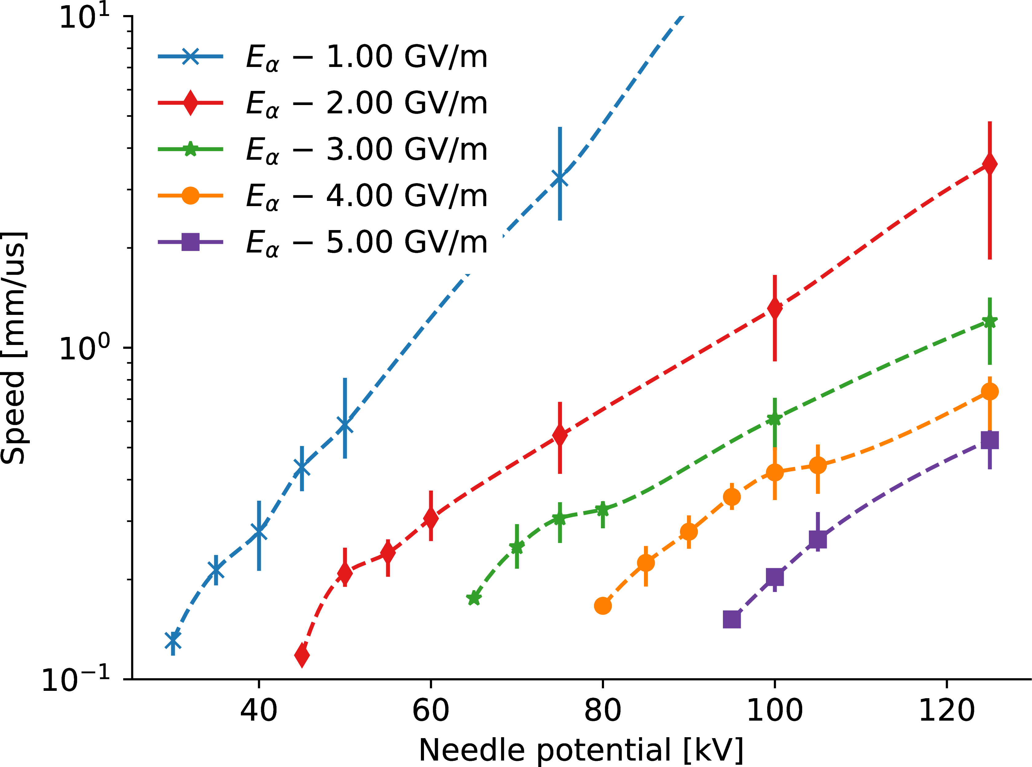
Figure 15: The effect of $E_{\alpha}$ on the average streamer propagation speed for the middle 50 % of the gap. The dashed lines are interpolated to the average, and the bars covers the minimum and maximum values.

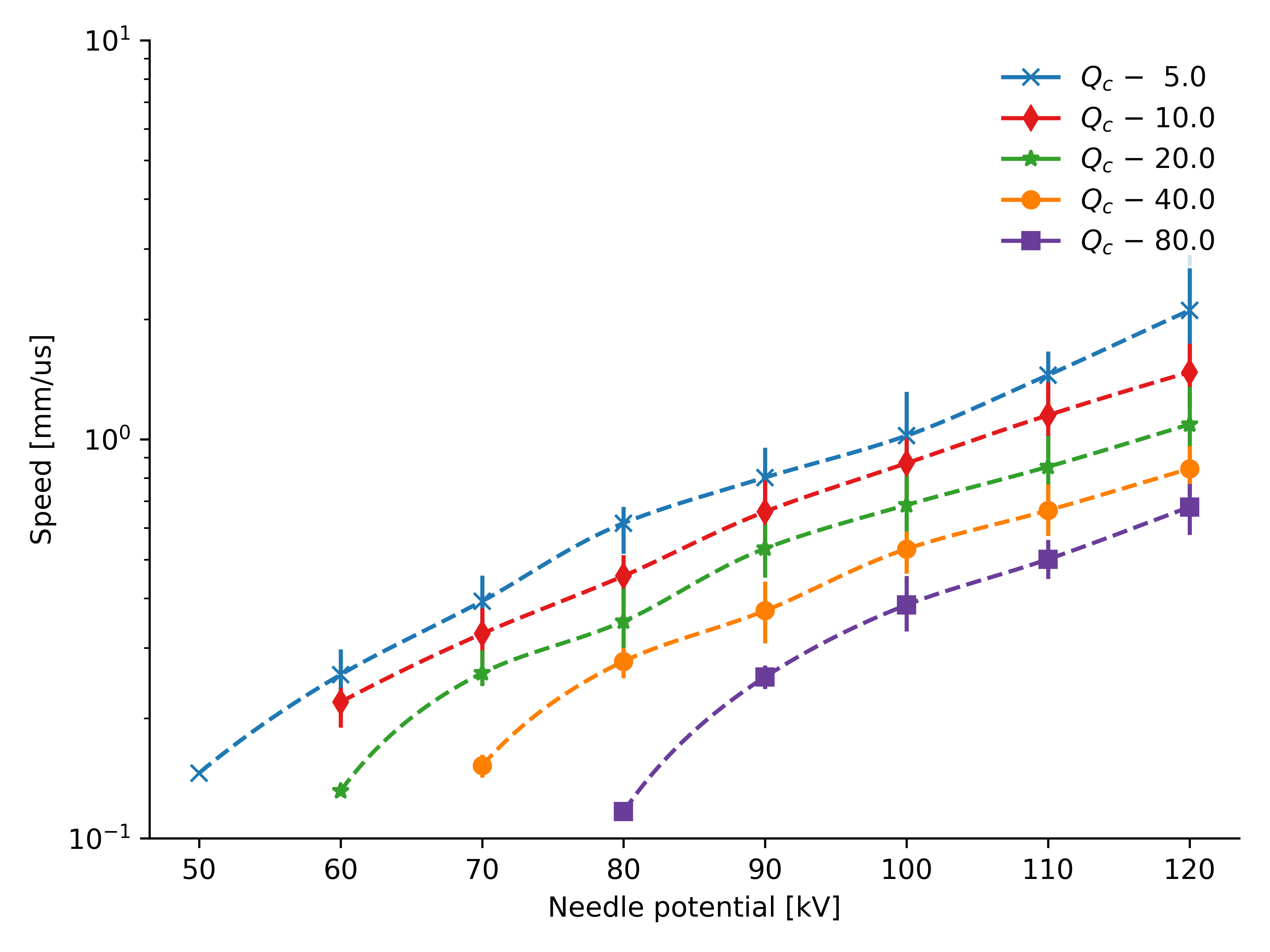
Figure 16: The effect of $Q_{\textrm{c}}$ on the average streamer propagation speed for the middle 50 % of the gap. The dashed lines are interpolated to the average, and the bars covers the minimum and maximum values.

The avalanche mechanism is the most important part of the model. For this reason, parameters relevant to the avalanche growth, given in 16 and 19, are especially important. To get an avalanche, however, a seed electron is needed. A doubling of the concentration of seeds $n_{\textrm{ion}}$, gives about a doubling in the propagation speed, as seen in figure 12. The figure shows the average speed for the mid 50 % of the gap, that is for a position from $0.75\text{\,}\mathrm{mm}2.25\text{\,}\mathrm{mm}$. Since streamers terminated in the first quarter of the gap are not shown, the figure also indicates that the breakdown voltage is dependent on $n_{\textrm{ion}}$, as increasing $n_{\textrm{ion}}$ allows propagation at lower voltages. The streamer is represented by one or more heads, and propagates as new heads are added in front of current heads. As such, the leading head moves in a series of discrete “jumps”. The average streamer head jump length seems independent of $n_{\textrm{ion}}$, indicating that the linear increase in propagation speed is caused by a reduction in the time required for an electron to become a critical avalanche. At $n_{\textrm{ion}}=$2\text{\times}{10}^{12}\text{\,}\mathrm{m}\mathrm{}{-3}$$, the average distance between seeds is $79\text{\,}\mathrm{\SIUnitSymbolMicro m}$, while the average jump length is about $6\text{\,}\mathrm{\SIUnitSymbolMicro m}$, so $n_{\textrm{ion}}$ would have to be increased by some orders of magnitude to affect the streamer jump distance. Inhomogeneities on the order of ${10}^{11}\text{\,}\mathrm{m}\mathrm{}{-3}$ was introduced by [37] to explain branching, but this effect is not found here. An upper estimate on the ions available can be calculated from 12 by using $G_{\textrm{ion}}$ instead of $G_{\textrm{free}}$ when calculating $R_{\textrm{e}}$ in 5 and using a low estimate of $k_{\textrm{r}}=${10}^{-3}\text{\,}\mathrm{m}\mathrm{m}\mathrm{}\mathrm{2}\mathrm{V}\mathrm{}{-1}\mathrm{s}\mathrm{}{-1}$$ [53, 37], yielding $n_{\textrm{ion}}=$1.8\text{\times}{10}^{13}\text{\,}\mathrm{m}\mathrm{}{-3}$$ and an average distance of $38\text{\,}\mathrm{\SIUnitSymbolMicro m}$ between seeds. As such, the simulations in figure 12 cover the most interesting range.

The baseline results in section 3.1 do not show any stopping of streamer propagation mid-gap. The streamers either stop within the first $100\text{\,}\mathrm{\SIUnitSymbolMicro m}$ or cause a breakdown. This occurs when the supply of electrons is constant and $E_{\textrm{s}}$ is too low to create a high voltage drop along the streamer. Increasing the electron detachment threshold $E_{\textrm{d}}$ reduces the number of electrons available, which in turn reduces the density of electrons as electrons are swept out, see figure 13. This results in a negative feedback loop where a lower density of electrons decreases the speed (figure 12) and the decreased speed results in a lower rate of ions turning into electrons. The propagation length is shown as a function of the needle potential and $E_{\textrm{d}}$ in figure 14. By considering $E_{\textrm{d}}=$15\text{\,}\mathrm{MV}\text{\,}{\mathrm{m}}^{-1}$$, three different regimes is identified. Up to $70\text{\,}\mathrm{kV}$, a few avalanches may occur, but then the propagation stops. Above $90\text{\,}\mathrm{kV}$, the propagation is fast enough to provide a stable rate of new electrons, enabling the propagation to continue. In between, the initial electrons allow the streamer to propagate, but the electron density is decreasing and the streamer eventually stops.

The electric field is important for electron movement and multiplication, and $E_{\alpha}$ in 16 is therefore an important parameter. The strong influence of $E_{\alpha}$ is seen in figure 15, where the propagation speed may increase by an order of magnitude when $E_{\alpha}$ is reduced by 50 %. This makes sense as $E_{\alpha}$ enters exponentially in 16. The propagation speed of 2nd mode streamers is weakly dependent on the applied voltage [2], however, for $E_{\alpha}=$1\text{\,}\mathrm{GV}\text{\,}{\mathrm{m}}^{-1}$$ in figure 15, the dependence is much stronger than for the other values. Reducing $E_{\alpha}$ facilitates streamer propagation and the breakdown voltage is thus strongly influenced. Both $E_{\alpha}$ and $\alpha_{\textrm{m}}$ are based on experimental results, and are very important to the model. Instead of varying $\alpha_{\textrm{m}}$, however, the Meek-constant $Q_{\textrm{c}}$ is varied. From 16, 18 and 19, it is clear that the avalanche size $Q_{\textrm{e}}$ is linearly dependent on $\alpha_{\textrm{m}}$, which implies that doubling $Q_{\textrm{c}}$ has the same effect as halving $\alpha_{\textrm{m}}$. The speed is not as affected by $Q_{\textrm{c}}$ as intuitively expected, see figure 16, and changing $Q_{\textrm{c}}$ by a factor of 4 only changes the speed by a factor of 2. However, $Q_{\textrm{c}}$ cannot change much before the simulation becomes unphysical. For instance, consider a conducting sphere of $r=$6\text{\,}\mathrm{\SIUnitSymbolMicro m}$$ with a charge $q=\exp(Q_{\textrm{c}})$. The electric field at the surface is

$$E=\frac{eq}{4\pi\epsilon r^{2}}\,,$$ (33)

where $e$ is the electron charge and $\epsilon$ is the permittivity. For $Q_{\textrm{c}}$ equal 15, 20, and 25, the electric field becomes $6.5\text{\times}{10}^{7}\text{\,}\mathrm{V}\text{\,}{\mathrm{m}}^{-1}$, $9.7\text{\times}{10}^{9}\text{\,}\mathrm{V}\text{\,}{\mathrm{m}}^{-1}$, and $1.4\text{\times}{10}^{12}\text{\,}\mathrm{V}\text{\,}{\mathrm{m}}^{-1}$, respectively. Increasing $Q_{\textrm{c}}$ by a little gives too high fields, and a decrease results in low fields. This can, however, be “fixed” by changing the radius. For instance, $Q_{\textrm{c}}=15$ and $r=$1\text{\,}\mathrm{\SIUnitSymbolMicro m}$$, results in $2.4\text{\times}{10}^{9}\text{\,}\mathrm{V}\text{\,}{\mathrm{m}}^{-1}$, which is more reasonable. To consider the electron avalanche as a charged sphere is of course a simplification, but the majority of the charge does build up over a length of some $\mathrm{\SIUnitSymbolMicro m}$, and this is also the size used for the streamer heads, which makes the analogy reasonable. While it would seem like increasing $Q_{\textrm{c}}$ does not make sense, one should remember that it actually has the same effect on the model as decreasing $\alpha_{\textrm{m}}$, and the value of that parameter is not certain. For instance, according to [22], $\alpha_{\textrm{m}}=$200\text{\,}{\mathrm{\SIUnitSymbolMicro m}}^{-1}$$, but [62] finds $\alpha_{\textrm{m}}=$130\text{\,}{\mathrm{\SIUnitSymbolMicro m}}^{-1}$$, however, the latter study also finds $E_{\alpha}=$1.9\text{\,}\mathrm{GV}\text{\,}{\mathrm{m}}^{-1}$$, and changing this parameter has a big impact on the model, as discussed above.

3.3 Effect of streamer parameters

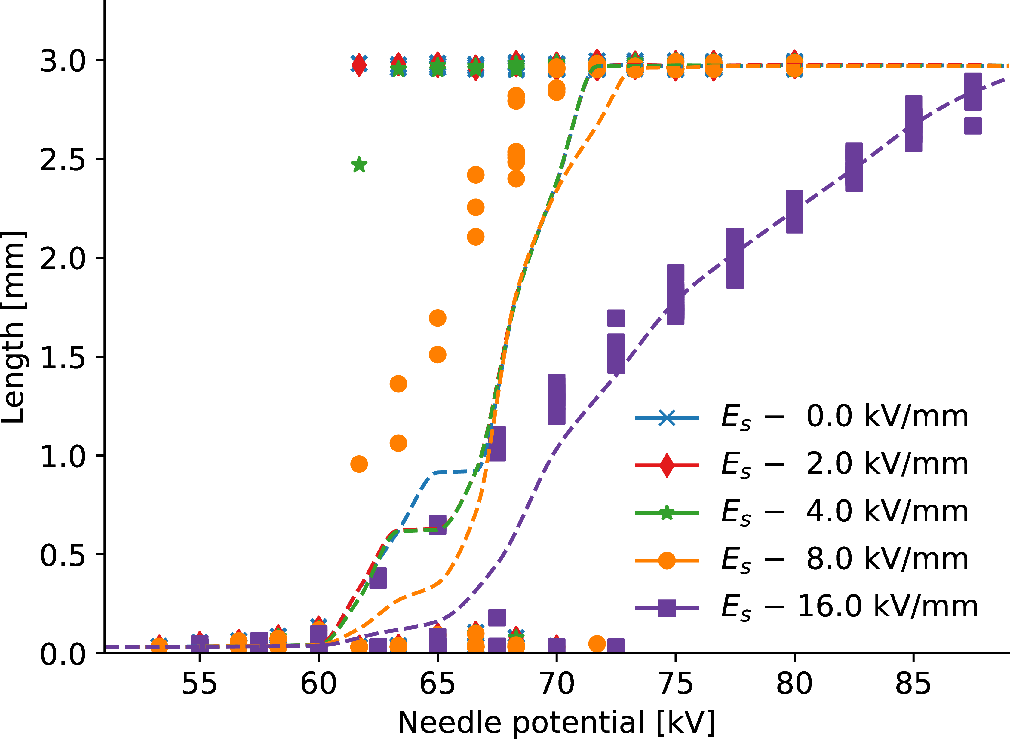
Figure 17: Streamer propagation length as a function of needle potential and electric field in streamer channel $E_{\textrm{s}}$. Each marker is a simulation and the dotted lines are interpolated to the average. Note that up to $8\text{\,}\mathrm{kV}\text{\,}{\mathrm{m}}^{-1}$, the results overlap to a high degree.

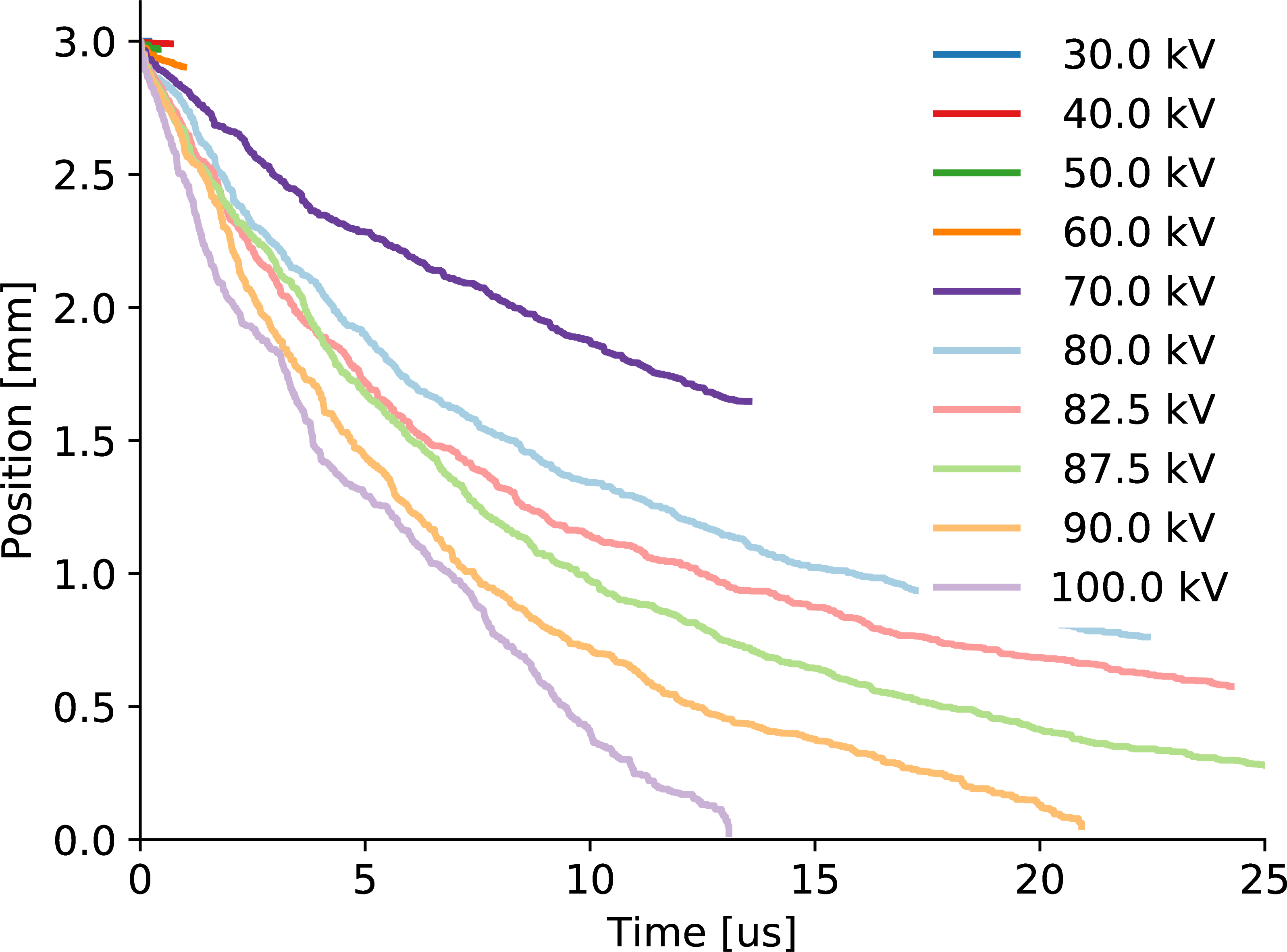
Figure 18: Streak plots of streamer leading head position, using $E_{\textrm{s}}=$16\text{\,}\mathrm{kV}\text{\,}{\mathrm{mm}}^{-1}$$, causing the streamers to slow down and sometimes stop.

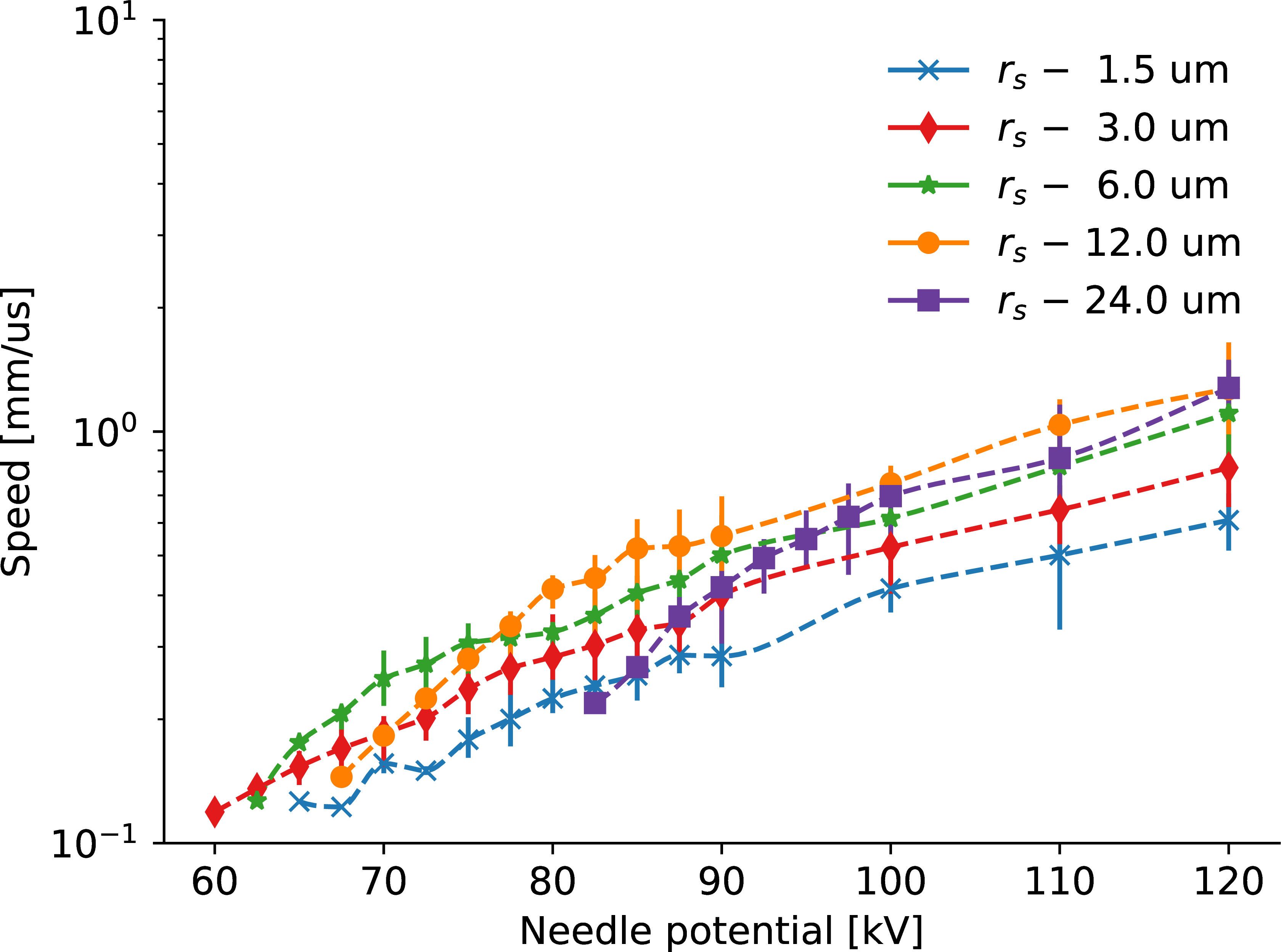
Figure 19: Streamer propagation speed for a series of different streamer head tip curvatures $r_{\textrm{s}}$. The dotted lines are interpolated to the average, and the bars covers the minimum and maximum values.

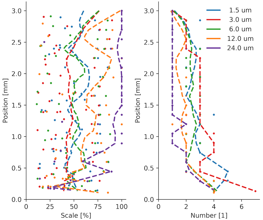
Figure 20: Actual streamer head scale $k_{i}$ (left) and total number of streamer heads (right) at $100\text{\,}\mathrm{kV}$ for a series of streamer head tip curvatures $r_{\textrm{s}}$. Data are taken every 5 % of the gap. The dashed lines are moving averages calculated by loess-regression [72].

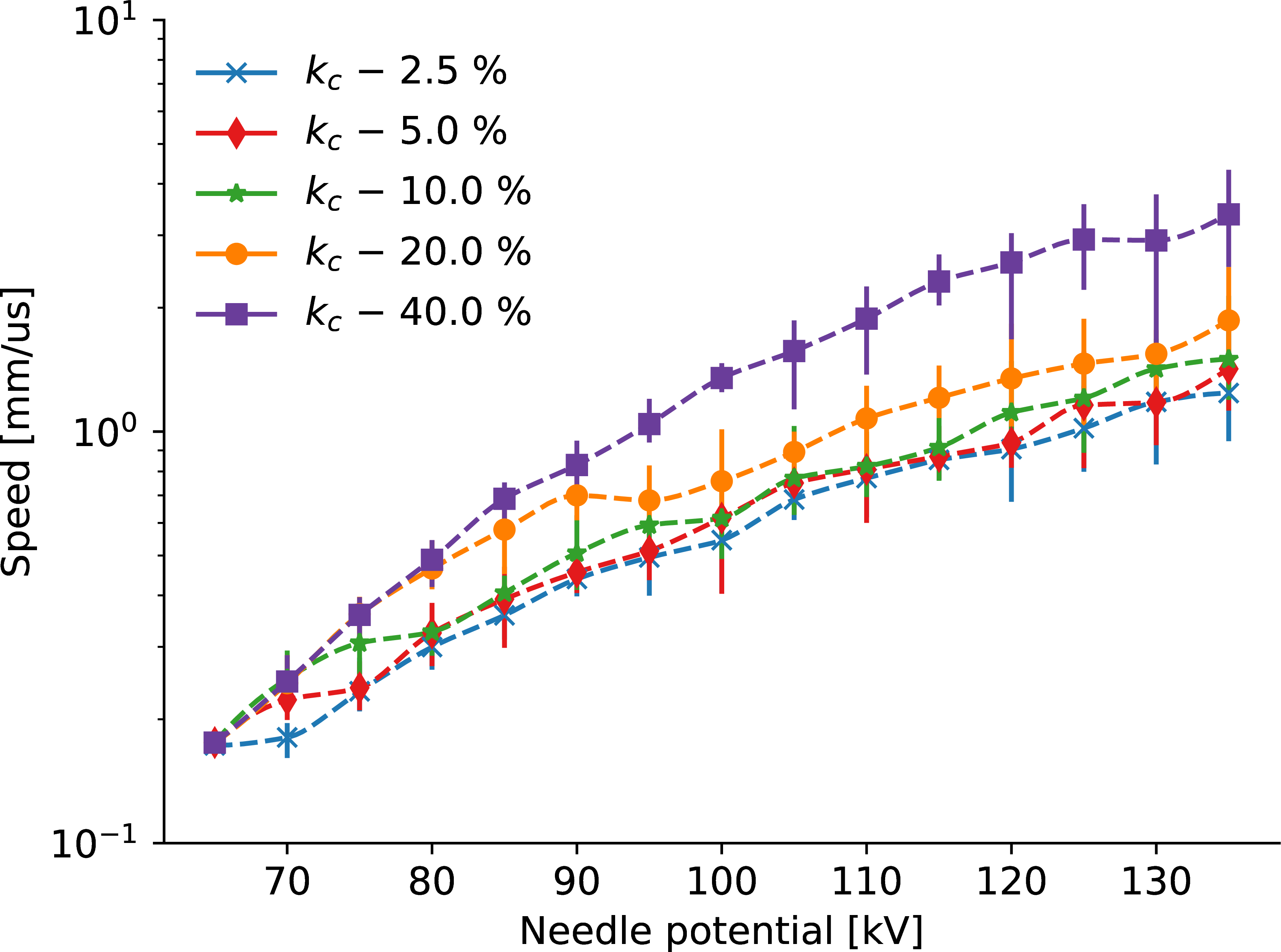
Figure 21: The effect of streamer head scale threshold $k_{\textrm{c}}$ on the streamer propagation speed, calculated for the mid 50 % of the gap. The dotted lines are interpolated to the average, and the bars covers the minimum and maximum values.

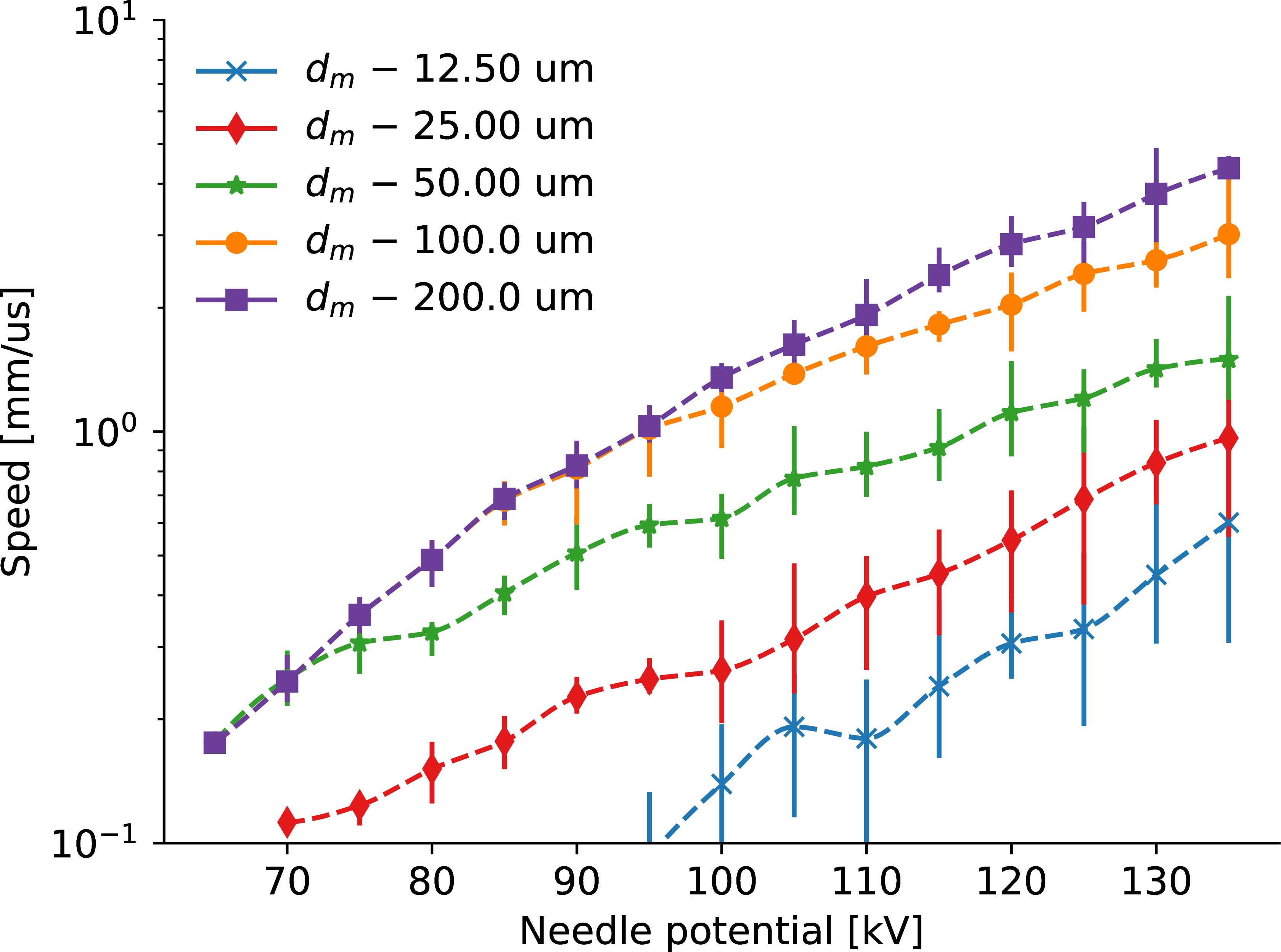
Figure 22: The effect of streamer merge distance $d_{\textrm{m}}$ on the streamer propagation speed, calculated for the mid 50 % of the gap. The dotted lines are interpolated to the average, and the bars covers the minimum and maximum values.

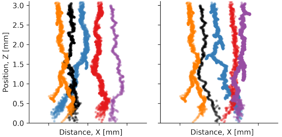
Figure 23: Streamer head positions for simulations at $120\text{\,}\mathrm{kV}$. Variation of $k_{\textrm{c}}$ (left): 10 % (yellow), 20 % (black), 2.5 % (blue), 5.0 % (red), and 40 % (purple). Variation of $d_{\textrm{m}}$ (right): $50.0\text{\,}\mathrm{\SIUnitSymbolMicro m}$ (yellow), $200\text{\,}\mathrm{\SIUnitSymbolMicro m}$ (black), $25.0\text{\,}\mathrm{\SIUnitSymbolMicro m}$ (blue), $100\text{\,}\mathrm{\SIUnitSymbolMicro m}$ (red), and $12.5\text{\,}\mathrm{\SIUnitSymbolMicro m}$ (purple).

The streamer structure is responsible for propagating the electric field from the needle into the gap. The electric field in the streamer channel $E_{\textrm{s}}$ gives a voltage drop from the needle to the streamer head. The electric field in front of a streamer head is also dependent on the tip radius of curvature $r_{\textrm{s}}$ and the potential scaling of the streamer head $k_{\textrm{i}}$. The scaling depends on the potential and position of all the streamer heads, that is, the entire “streamer”. Both the streamer head merge distance $d_{\textrm{m}}$ and the potential shielding threshold $k_{\textrm{c}}$ may be important for the streamer configuration.

Figure 14 demonstrates streamers stopping as a result of a reduction in the seed electron density, however, it is common to explain stopping as a result of an electric field $E_{\textrm{s}}$ in the streamer channel resulting in a lower field strength at the streamer head [26]. A high $E_{\textrm{s}}$ is needed to affect the results (see figure 17), conversely, when $E_{\textrm{s}}$ is low, the streamer either stops quickly or causes a breakdown. When $E_{\textrm{s}}$ is high, the propagation speed is reduced throughout the gap and the propagation may stop somewhere in the gap, see figure 18 for $E_{\textrm{s}}=$16\text{\,}\mathrm{kV}\text{\,}{\mathrm{mm}}^{-1}$$, which is in contrast to figure 7 for $E_{\textrm{s}}=$2.0\text{\,}\mathrm{kV}\text{\,}{\mathrm{mm}}^{-1}$$ where the streamers do not stop. Both figures 17 and 18 indicate that $E_{\textrm{s}}$ is not important in the beginning of the propagation, but becomes important when a streamer has reached some length. When $E_{\textrm{s}}=$8\text{\,}\mathrm{kV}\text{\,}{\mathrm{mm}}^{-1}$$, the potential is reduced by $24\text{\,}\mathrm{kV}$ across the gap, but this effect is barely seen (figure 17), since only a few streamers stop mid-gap. However, at $16\text{\,}\mathrm{kV}\text{\,}{\mathrm{mm}}^{-1}$ the effect is clearly present as many of the streamers stop mid-gap. Notice that at $75\text{\,}\mathrm{kV}$ to $85\text{\,}\mathrm{kV}$, in figure 17 the average propagation length is increased from about $1.7\text{\,}\mathrm{mm}$ to $2.6\text{\,}\mathrm{mm}$, giving an apparent electric field of only $11\text{\,}\mathrm{kV}\text{\,}{\mathrm{mm}}^{-1}$ and not $16\text{\,}\mathrm{kV}\text{\,}{\mathrm{mm}}^{-1}$. This is perhaps an effect of the field increasing as the gap is getting smaller. Also, actual experiments show stopping lengths that are increasing linearly with voltage in the first part of the gap, followed by more scatter and superlinear behavior towards the end of the gap [66, 15, 11]. This behavior is not seen in figure 17, possibly because $E_{\textrm{s}}$ is kept constant in the simulations, while it has been found to vary with applied voltage [8]. Streamers are subject to re-illuminations, associated with current pulses, which could change the electric field in the streamer channel, however, the propagation of the streamer head seems to be unaffected by these effects [8].

The curvature radius $r_{\textrm{s}}$ of a streamer head is an interesting parameter since a sharper tip gives a higher field and a larger volume where electron multiplication may occur. Changing $r_{\textrm{s}}$ from $1.5\text{\,}\mathrm{\SIUnitSymbolMicro m}$ to $12\text{\,}\mathrm{\SIUnitSymbolMicro m}$ only changes the speed by a factor of 2, see figure 19. Further increase to $24\text{\,}\mathrm{\SIUnitSymbolMicro m}$ decreases the speed, and increases the breakdown voltage. Simulations with smaller $r_{\textrm{s}}$ tend to have more streamer heads, scaled to a lower potential, than the simulations with a larger $r_{\textrm{s}}$, indicated in figure 20, although the effect is not visible for the smallest $r_{\textrm{s}}$ in that figure. The increased number of streamer heads seems to act as a regulating mechanism, however, the number of branches is not increased, but there are more streamer heads present simultaneously in the same branch. This is similar to the situation in figures 9 and 10, where an increased voltage does not increase the number of branches, but instead increases the streamer thickness.

An increase in voltage increases the speed (figure 8) as well as the number of streamer heads, while decreasing the scaling of the heads as demonstrated in figure 10. The parameters $k_{\textrm{c}}$ and $d_{\textrm{m}}$ are used to remove streamer heads, and therefore they could have a big impact on the model, since the scaling, which the electric field depends on, is strongly dependent on the number of streamer heads as well as their configuration. Also, these parameters are purely a consequence of the model, and do not have an origin in a physical property. Simulation results for varying $k_{\textrm{c}}$ are found in figure 21 and show that the propagation speed is not that affected, except for $k_{\textrm{c}}=40~{}\%$. This figure also indicates that the breakdown voltage is unaffected, since all the values of $k_{\textrm{c}}$ are present for all the voltages. Setting $k_{\textrm{c}}=40~{}\%$ restricts the streamer to one head in most situations, and keeping two heads in rare occasions, which gives an upper bound to the propagation speed for each voltage. From a computational point of view, it is preferable to set $k_{\textrm{c}}$ high as fewer streamer heads implies less calculation. From a physical point of view, however, it does not make sense to just remove charges from the system, so $k_{\textrm{c}}$ should be reasonably low. According to figure 21, $k_{\textrm{c}}$ can be as high as 10 % without any particular impact on the results.

The influence of the streamer head merge distance $d_{\textrm{m}}$ is shown in figure 22. For the lower values, many streamer heads are present at the same time, which in turn lowers the potential scaling of each head, increases the breakdown voltage, and moderates the propagation speed. Increasing $d_{\textrm{m}}$ increases propagation speeds, up to the limit where there is mainly just a single active streamer head. Figure 22 also indicates that at low voltages, the streamers propagate with a single head, but when the voltage is increased and more heads are possible, the propagation speed is moderated. As $d_{\textrm{m}}$ is increased, the voltage needed to have several heads is also increased, and the propagation speed is thus higher. The set of streamers presented in figure 23 shows that the thickness of the streamers is dependent on $k_{\textrm{c}}$ and $d_{\textrm{m}}$, which is an indication of the number of streamer heads present during propagation. However, the figure does not indicate a change in the number of major branches.

3.4 Effect of additives

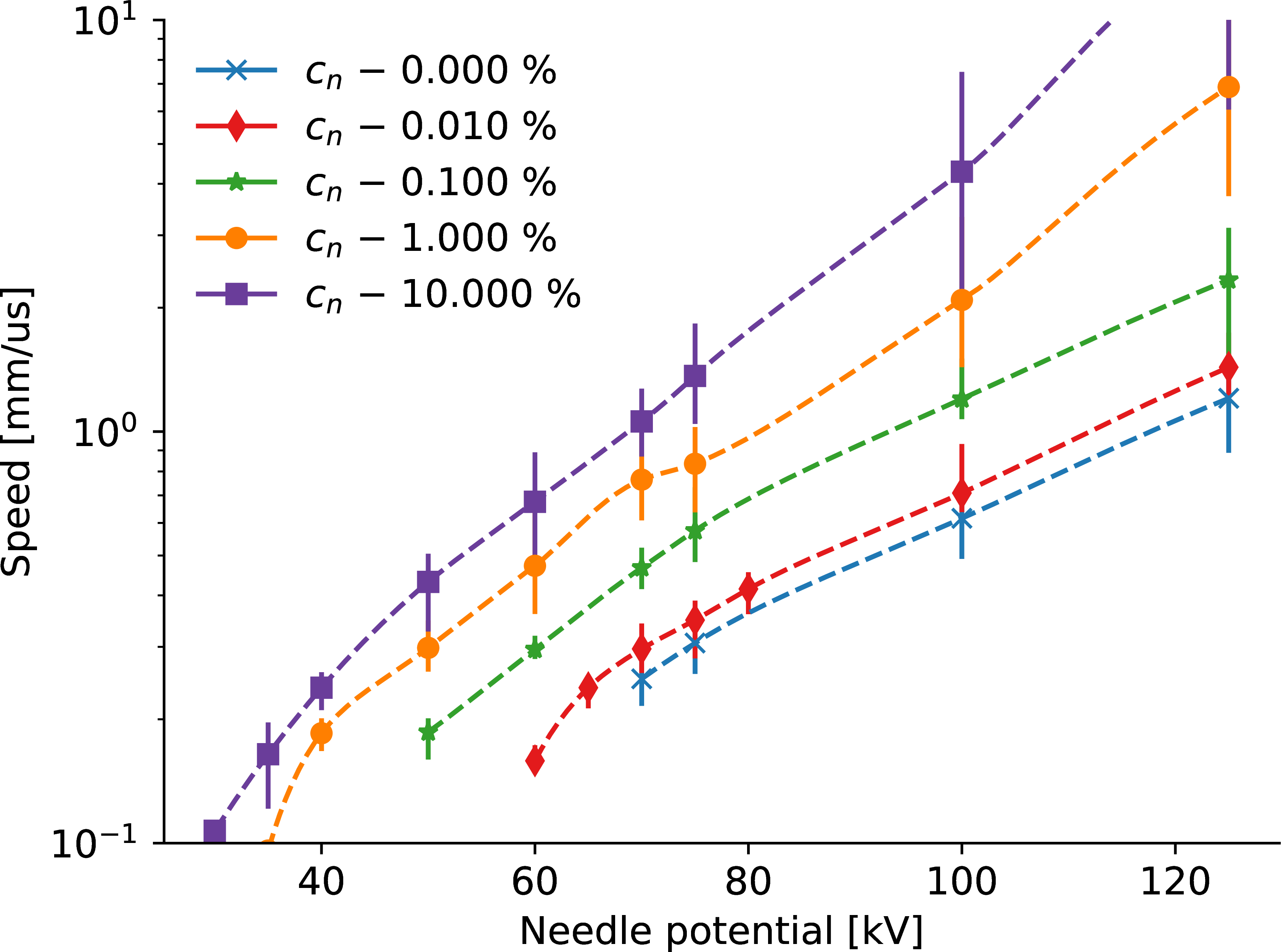
Figure 24: Streamer propagation speed for various fractions of added additive $c_{\textrm{n}}$. Average speed for the middle 50 % of the gap. Each marker is a simulation and the dotted lines are interpolated to the average.

Adding small amounts of an additive increases the electron multiplication according to 20. The effect should be similar to an increase of $\alpha_{\textrm{m}}$, or a decrease in $Q_{\textrm{c}}$, as discussed above and shown in figure 16. This is indeed the case, the propagation speed increases and the breakdown voltage decreases with increasing content of an additive with low ionization potential, see figure 24. When the liquid consists of $c_{\textrm{a,n}}=10~{}\%$ additive (mole fraction) it cannot be argued to be a “small amount” of additive. Even as little as 1 % could be too much. As mentioned in section 2.4, an addition of just 0.1 % increases the avalanche growth by a factor of 6.9, when using 20 and the parameters in table 1. A decrease in breakdown voltage and an increase in propagation speed is also found in experiments with low-IP additives [3, 41, 11], however, increased branching is also seen in the experiments in contrast to the simulation results here.

3.5 Increased speed and branching

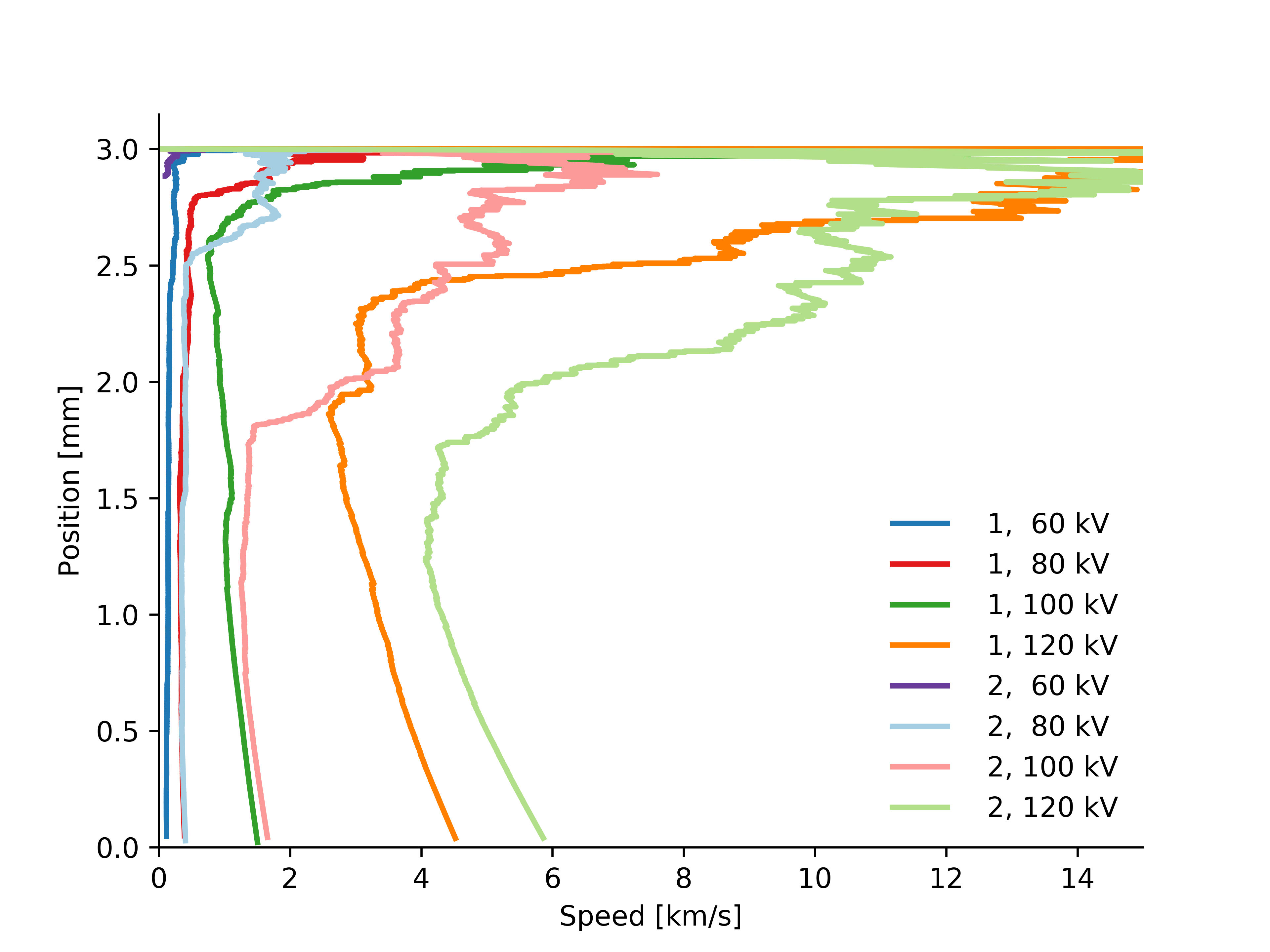
Figure 25: Streamer average speed versus leading head position. The simulations at the same voltage differ only by the initialization of the random number generator.

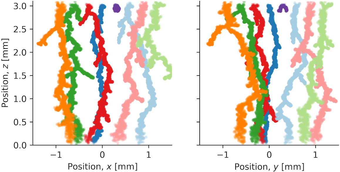
Figure 26: Streamer trails for a range of voltages, using the same colors as in figure 25. Each dot represents the position of a streamer head at some point of the propagation.

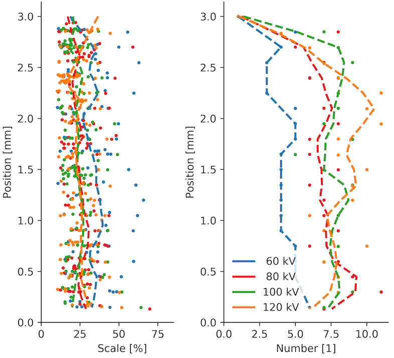
Figure 27: Actual streamer head scale $k_{i}$ (left) and total number of streamer heads (right). Data are taken every 5 % of the gap. The dashed lines are moving averages.

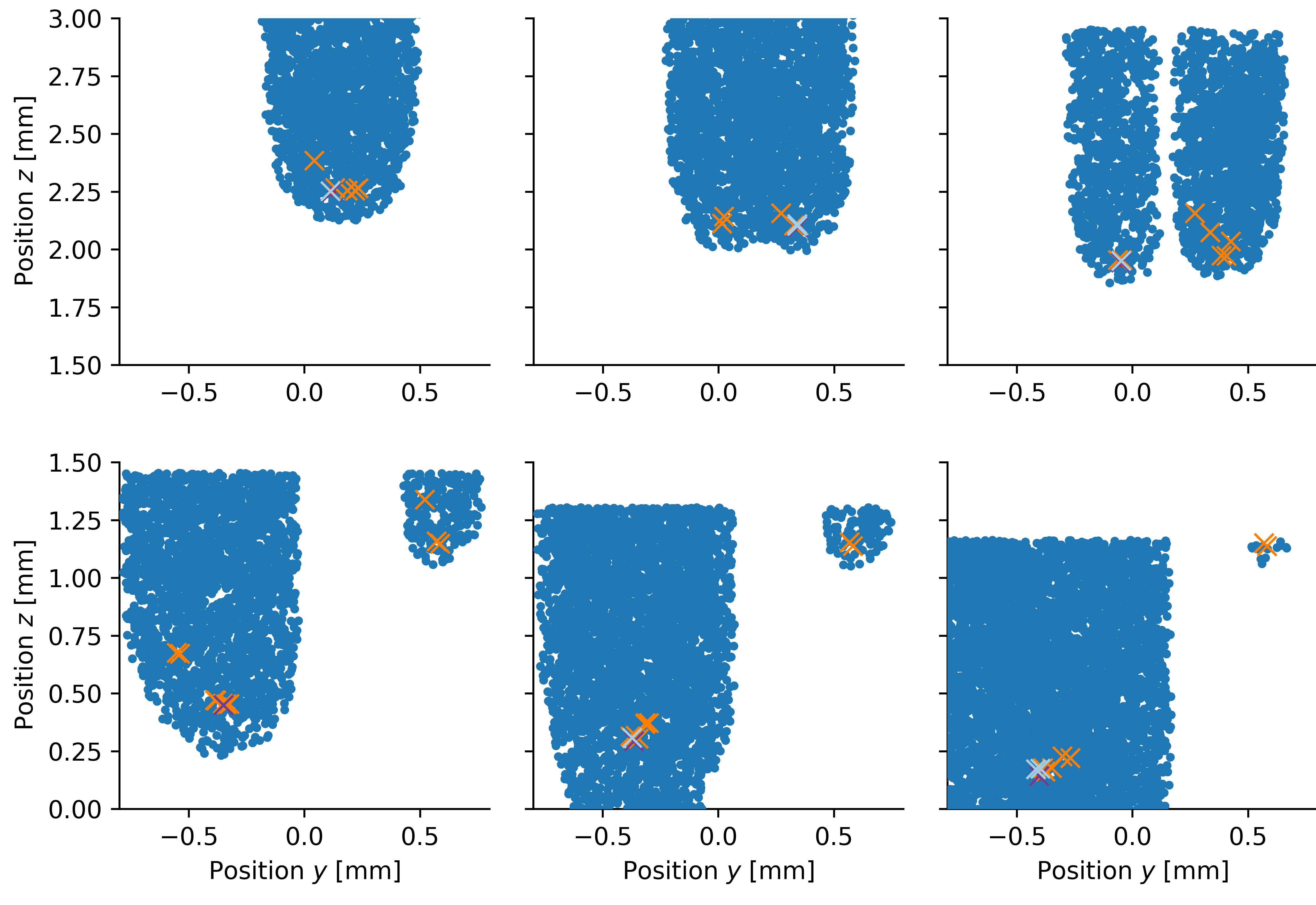
Figure 28: Detailed illustration of streamer branching. The electron avalanches are shown as blue dots, and the streamer head as crosses. The top three plots show streamer bifurcation in the start of the gap, while the bottom three plots show one propagating branch and another stopped branch at the end of the gap.

The above sections illustrate how the model behaves and how it is affected by the various parameters. In order to reduce the initiation voltage and increase the propagation speed, the avalanche parameters are changed to $E_{\alpha}=$1.9\text{\,}\mathrm{GV}\text{\,}{\mathrm{m}}^{-1}$$ and $\alpha_{\textrm{m}}=$130\text{\,}{\mathrm{\SIUnitSymbolMicro m}}^{-1}$$, and the number of seeds is increased to $c_{\textrm{s}}=$8\text{\times}{10}^{12}\text{\,}\mathrm{m}\mathrm{}{-3}$$. In addition, the merge distance is changed to $d_{\textrm{m}}=$12.5\text{\,}\mathrm{\SIUnitSymbolMicro m}$$ and the streamer head tip radius to $r_{\textrm{s}}=$3\text{\,}\mathrm{\SIUnitSymbolMicro m}$$ in order to facilitate branching. Also, using $E_{\textrm{s}}=$8\text{\,}\mathrm{kV}\text{\,}{\mathrm{mm}}^{-1}$$ should be enough for some of the streamers to stop mid-gap. Most of the predicted results are found: the speed in figure 25 is clearly increased compared to figure 8, the amount of small branches is larger in figure 26 than in figure 9, and the decrease in streamer head scaling and increase in streamer head number is seen by comparing figure 27 to figure 10. The propagation voltage is somewhat lower than the base case, around $60\text{\,}\mathrm{kV}$. The streamer propagation begins at high speed, then slows down towards the middle of the gap, before the speed increases towards the end of the gap, see figure 25. This change does not seem to be correlated to the number of streamer heads, which is fairly constant for most of the propagation (figure 27). Branching may have an effect, and streamer branching is illustrated in figure 28, showing 6 snapshots of a single simulation. As the streamer splits into two major branches, the number of electron avalanches surrounding the streamer heads decreases. The branches propagate at different speeds, and the faster one gains a higher potential and thus creates more electron avalanches. As the two branches approaches the end of the gap, one gains speed, while the other one stops.

4 Discussion of the model

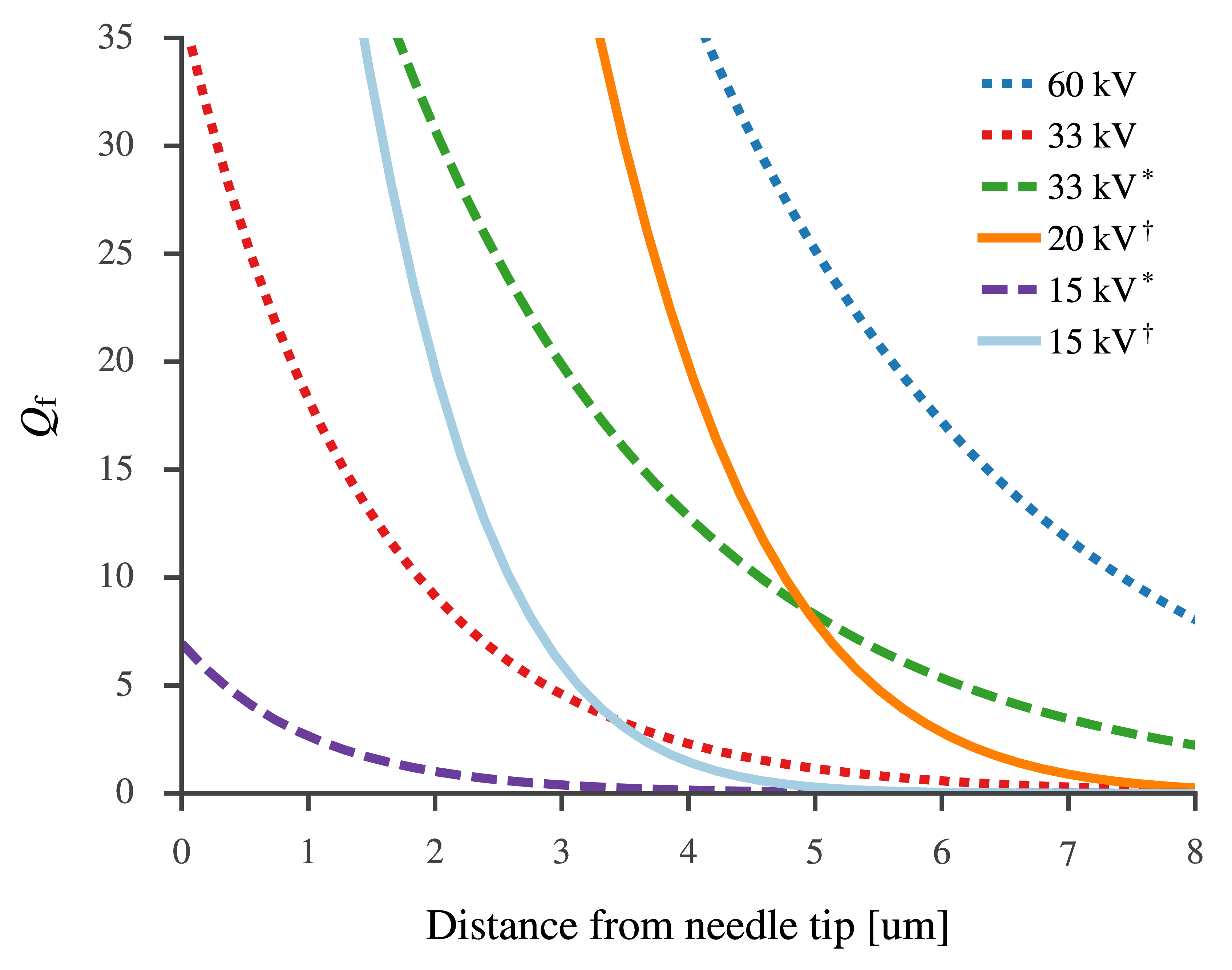
Figure 29: Maximum avalanche size at a distance from the needle tip. The unmarked lines use the same values as the baseline simulations from [22], the $*$ indicates parameter values from [62] as used in section 3.5, and the $\dagger$ indicates formulation and parameter values from [61].

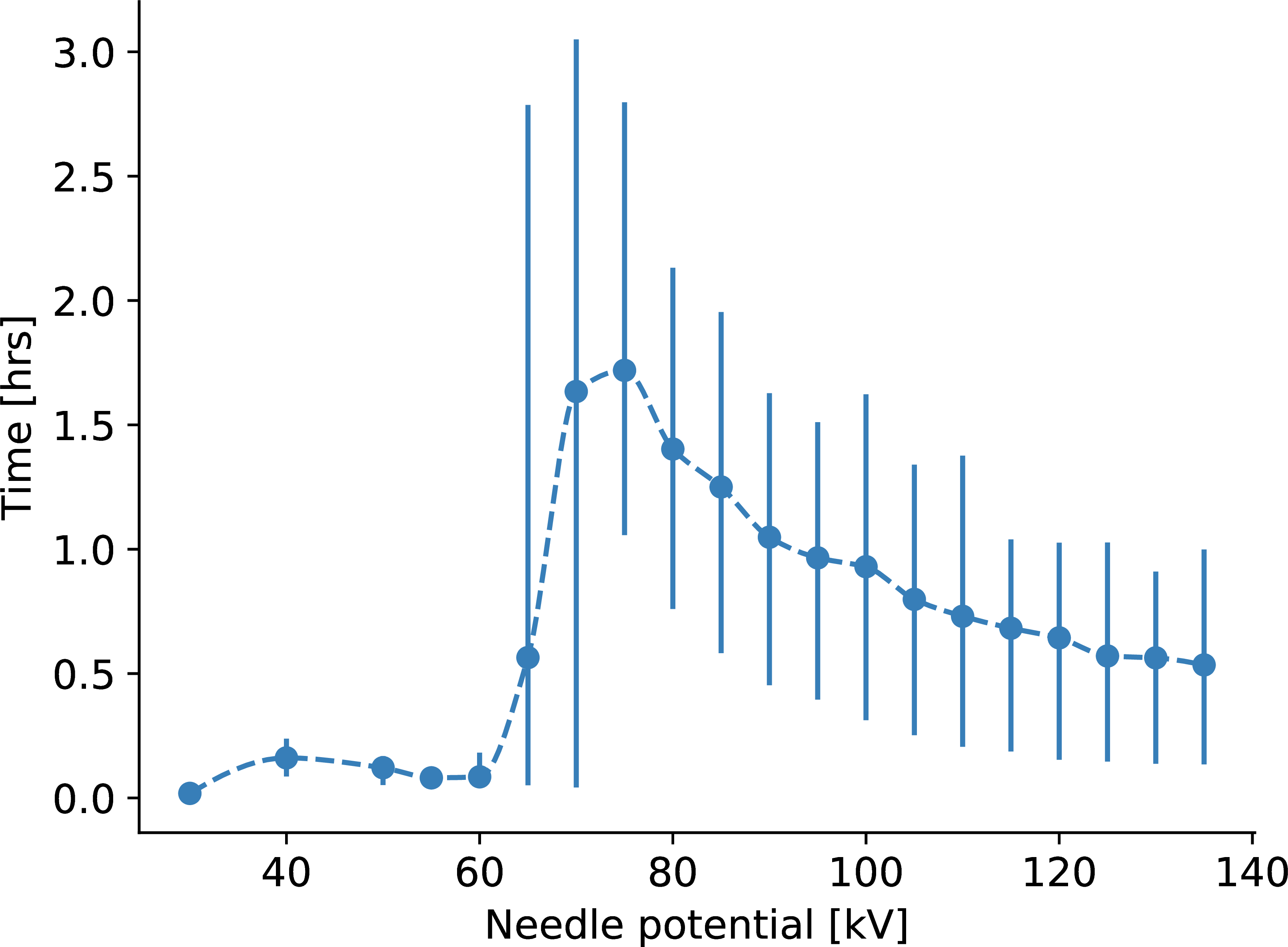
Figure 30: Total computational time for the simulations shown in figure 21 Streamers that terminate in the beginning of the gap require little time, while streamers that slowly bridges the gap requires the most computational time.

Using a Laplace field is of course a simplification compared to a Poisson field. In fact, neither positive nor negative charges are accounted for in the model. The potential is simply calculated by assuming a constant field in the streamer channel, and then superimposing the streamer heads. Including the charge of the avalanches and the ions left behind could improve the model. For the needle and the streamer heads, using a space charge limited field (SCLF) [73, 74] would provide a more physically correct field distribution, but would also increase the computational requirements drastically. Using an SCLF rather than a Laplace field, gives a reduction of the electric field where the field is the strongest, since the maximum field is limited [73], with a corresponding increase everywhere else. The SCLF is time-dependent [74], and the effect increases with time until an steady-state is obtained. The overall effect on the model would be an increase in average jump length, as most jumps would be longer and the shortest ones would not occur. While an SCLF can give more accurate results for slow streamers, a Laplace field could be good enough for fast streamers, since the SCLF-region expands at some finite speed. However, the avalanche parameters in 16 were estimated using a Laplace field, so the current model is internally consistent.

The inception of 2nd mode streamers has been estimated to somewhat less than $15\text{\,}\mathrm{kV}$ for cyclohexane [5], however, for a propagating 2nd mode streamer, $33\text{\,}\mathrm{kV}$ was found for a $10\text{\,}\mathrm{mm}$ gap [11]. Since the model uses this as a criterion for inception (getting a critical avalanche, but no movement), a high propagation voltage is actually to be expected. This is well illustrated by the maximum avalanche size in figure 29, obtained by integration of $\alpha$. Streamer propagation is possible when $Q_{\textrm{f}}>Q_{\textrm{c}}$ (cf. 19). The baseline simulations are performed inserting parameters from [22] in 16 to calculate $\alpha$. At $33\text{\,}\mathrm{kV}$, the maximum possible streamer jump is less than a $\mathrm{\SIUnitSymbolMicro m}$, however, at $60\text{\,}\mathrm{kV}$ (the breakdown voltage), the value is increased to about $6\text{\,}\mathrm{\SIUnitSymbolMicro m}$, possibly indicating that a strong field is needed over some distance. Changing to parameters from [62] decreases the propagation voltage by increasing the possible jump length, however, the decrease is not enough to enable for inception of 2nd mode streamers at $15\text{\,}\mathrm{kV}$. As such, figure 29 indicates that streamer inception at $15\text{\,}\mathrm{kV}$ is not possible with this model when considering a Laplace field, calculating the electron multiplication with 16, and using the Townsend–Meek criterion for inception of 2nd mode streamers. Using the parameters of either [22] or [62] gives too low avalanche size. According to [61], the correct way of calculating electron multiplication in a dense medium is

$$\alpha=\frac{3IE_{\nu}^{2}}{eE}\exp\left({-\frac{E_{\nu}^{2}}{E^{2}}}\right)$$ (34)

where $I$ is the ionization potential, $e$ is the electron charge, and $E_{\nu}$ is given by properties of the liquid. With this formulation, electron multiplication is more dependent on the electric field, implying that the electron avalanches become shorter, are closer to the streamer heads, and grow faster where the field is strong, which is illustrated in figure 29 using values for n-hexane [61].

The propagation velocity is somewhat low, which is to be expected since the inception voltage is too high. Changing parameters to values that lowers the inception voltage also increases the speed at a given voltage. As mentioned, the speed is proportional to the electron mobility, and it is the low-field mobility that has been used. For low-mobility liquids, such as cyclohexane, the mobility is expected to have a superlinear dependence on the electric field [56, 49]. For this reason, one study multiplies the mobility by 2.5, to make it similar to the gas phase mobility [38], which would increase the streamer propagation speed by the same factor. Conversely, limitations to the maximum speed of electrons have been introduced [75], which would effectively control the maximum speed of a streamer branch. The speed is also proportional to the concentration of seeds (see figure 12), which was calculated from the low-field conductivity of the liquid (see 10). However, for breakdown in non-polar liquids, the conductivity is not important [2], and hence, it seems unreasonable for this parameter to be as important as demonstrated here. The equilibrium density of ions can also be calculated based on cosmic radiation 17, but obtaining $>${10}^{11}\text{\,}\mathrm{m}\mathrm{}{-3}$$ ions, when the production is $\sim${10}^{8}\text{\,}\mathrm{m}\mathrm{}{-3}\mathrm{s}\mathrm{}{-1}$$, implies that a long time is needed. It is therefore an approximation to simulate a situation where this density is kept constant. By changing the simulation conditions such that all the gap is included in the ROI and such that seeds are not replaced, it can be verified that the seeds present at the beginning of the experiment is not enough. They are swept out very fast if they are electrons and not ions. Increasing $E_{\textrm{d}}$ so that most seeds remain as anions changes this by allowing the low-mobility anions to live longer before entering the high-field area and ionize into molecules and electrons. Even so, it seems clear that some mechanism for generation of new seeds is warranted. New seeds could be generated in the high-field areas, and near the electrodes. The Zener model [76] (field-ionization) for breakdown in solids has been used also for charge generation in liquids [24, 37]. Photoionization could also have an important role in the generation of new charges [9, 2], and adding field ionization and photoionization could improve the model. In addition, when ionizing neutral molecules, the field-dependent ionization potential [13] should also be taken into account. This kind of additions add complexity to the model, but Monte Carlo (MC) [77] methods can aid in keeping the added computational cost low. There are also some parts of the current model where MC could be reasonable to use. For instance, for electron detachment from an anion and for avalanche growth from a single electron, since a large number of electrons is needed to model an avalanche through the average growth $\alpha$.

The degree of branching is lower than desired, with more or less only one major branch, and thus the simulations resemble more the 3rd mode or the start of the 4th mode than the 2nd mode of a streamer. It is worthwhile noting that streamers branch far less in cyclohexane than in mineral oil, but the addition of low-IP additives increases the branching [41]. The shapes of the simulated streamers do resemble the shape of streamers in longer gaps [41], however, while including additives in the model increases the propagation speed, the degree of branching is not increased. Although branching is thought of as a mechanism for regulating the propagation speed, it could be the other way around. With nothing to hold it back, the foremost head should have the strongest electric field and the fastest propagation. If something is regulating the speed or field of the foremost head, however, then other heads are given a better chance of propagation, increasing the number of branches, which in turn may regulate the electric field of all the branches. In the present model, there is nothing holding the foremost head back, since the only time scale included is that of the electron avalanches. If, for instance, the time required for bubble nucleation or the time for charges to move through the streamer structure (streamer dynamics) is important, it may result in a disadvantage for the foremost head. This is, however, not included, and the potential of each streamer head is instantly updated each simulation step. The shape chosen for the streamer heads could also be a major reason for the low degree of branching. For a hyperboloid, the electric field declines as $r^{-1}$ in front, and the high-field region extends much further in the front than on the sides. Conversely, the field from a monopole declines like $r^{-2}$ in all directions, and could as such facilitate branching. In such a model, however, the high field would be in a region closer to the streamer heads, making an SCLF approach even more relevant.

The simplicity of the presented model comes with several limitations, as discussed above, however, a simple model is also a good place to start. It makes it possible to identify whether a certain mechanism is important or not at a relatively low computational cost. Consider figure 30, which shows that the computational time for breakdown streamers averages to about one hour, using a single core on a regular desktop computer. The simulation time is of course strongly dependent on the number of seeds, streamer heads, and simulation steps, but with such a low base case, it is possible to perform a lot of simulations to gather statistics on a normal desktop computer. Contrary to lattice models, the presented model is based on physical processes, and the results are thus easier to evaluate. FEM models may be better in the end, but for now, such models cannot model a complete breakdown. They are also simplified, for example in the sense that phase changes are not accounted for [75]. Both lattice and FEM models demands much computational power and the mesh size becomes an important parameter, however, this is avoided in the model presented. Instead of dealing with processes at discrete point or in discretized elements, the model deals with discrete points that move. This approach makes sense when considering charge generated by electron avalanches at some distance from the streamer structure, or a streamer moving in discrete steps. For details on processes inside or very close to the streamer, however, a FEM approach seems more reasonable, and could provide valuable input to models on a larger scale.

5 Conclusion

A simple simulation model for streamer propagation has been presented. The streamer is represented by a collection of hyperbolic streamer heads, and is responsible for propagating the electric field from the needle electrode. In high-field areas, electrons detach from ions present in the liquid, and may turn into avalanches. If an avalanche meets the Townsend–Meek criterion, a new streamer head is added at its position, causing the streamer to propagate. As demonstrated, the model has some limitations, the inception voltage is too high while the degree of branching is low. These issues are discussed and explained, and directions for a systematic way of further developments are described. The main feature missing in the model is a proper representation of the dynamics of the streamer channel, however, the charge generation and the electric field calculation can be improved as well. The approach to streamer propagation applied here is different from that used by other models. The principle behind the model is simple, it is founded on physical mechanisms, and provides interesting information about how an avalanche-driven breakdown may occur. The simple model has its advantages in that it can be used to identify important mechanisms, without demanding excessive computational power.

Appendix A Prolate Spheroid Coordinates

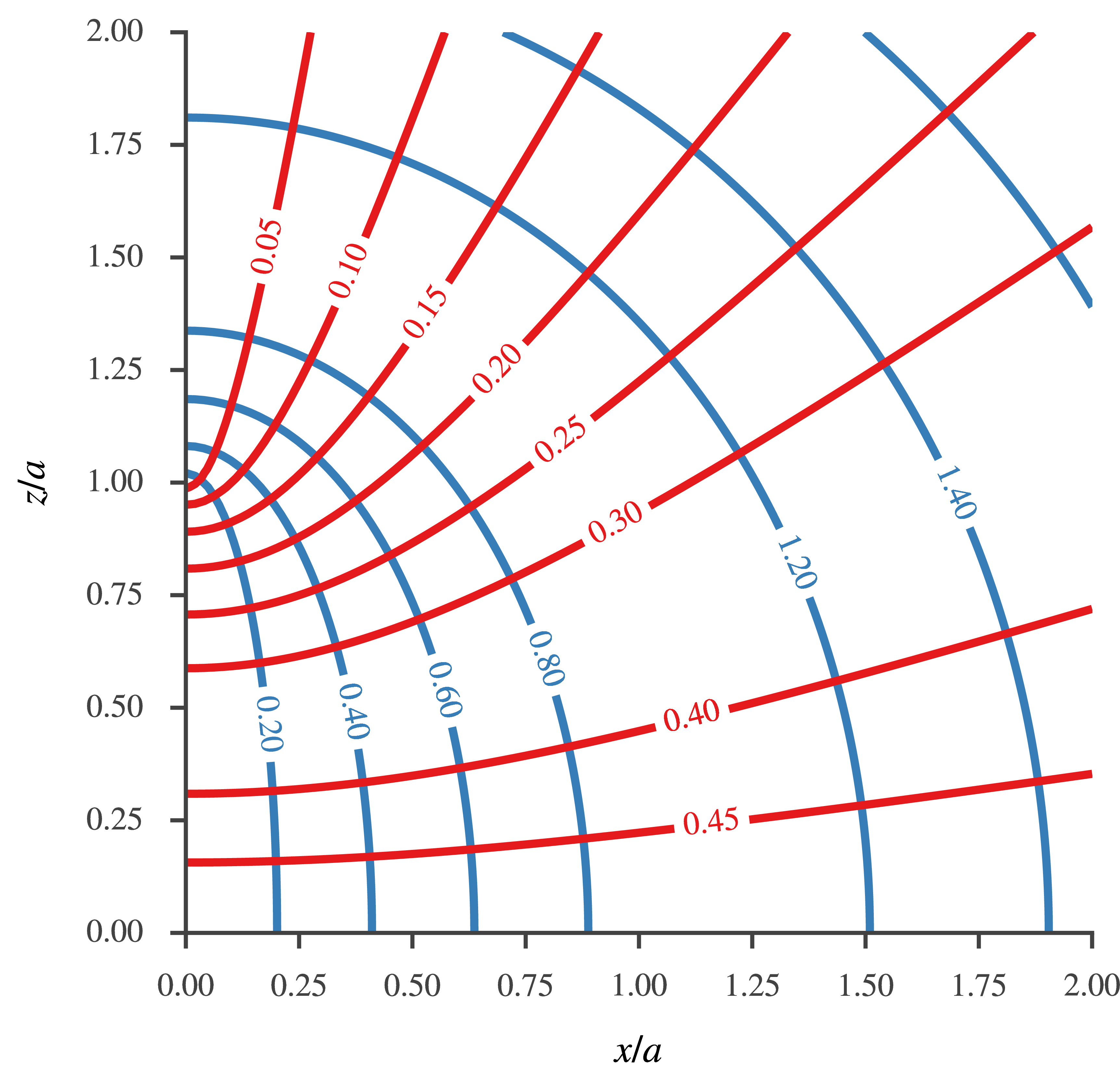
Figure 31: In prolate spheroid coordinates, spheroids (blue) are given by a constant $\mu$, and hyperboloids (red) have a constant $\nu$. Here, $\nu$ is given in units of $\pi$.

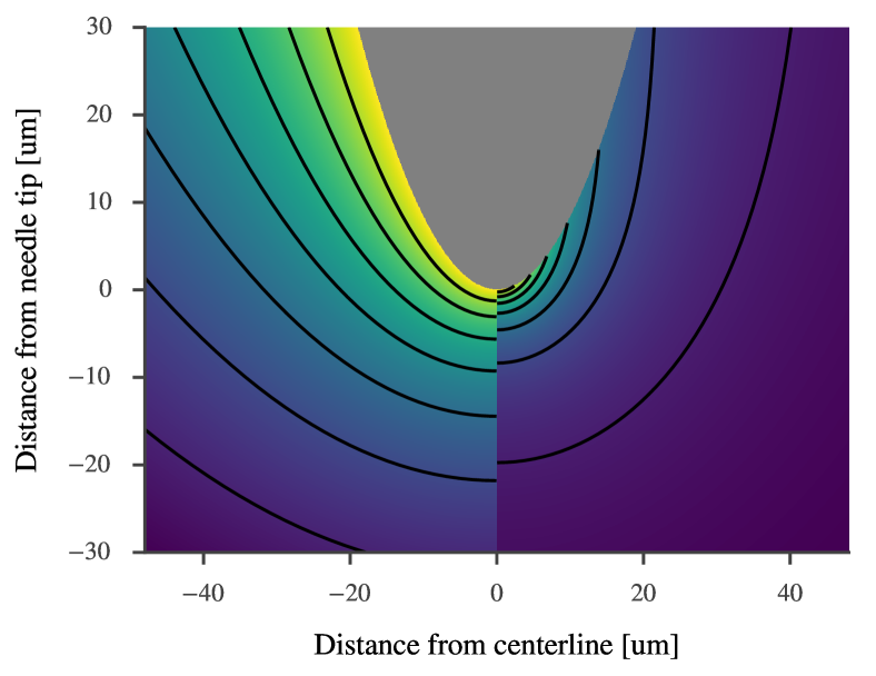
Figure 32: Electric potential (left) and electric field strength (right), for a region close to a needle (center, gray) placed $10\text{\,}\mathrm{mm}$ from a grounded plane. The contour lines give a qualitative impression of how the respective magnitudes change as a function of position. A linear scale is used for both sides, and the magnitudes are linearly dependent on the potential of the needle.

Prolate spheroid coordinates involves a set of hyperbolas and ellipsoids revolved around the center axis, forming hyperboloids and prolate spheroids. The two focal points, of the hyperbolas as well as ellipsoids, are located at a distance $a$ from the plane. The hyperbolic coordinate is $\mu\in[0,\infty\rangle$, the elliptic coordinate is $\nu\in[0,\pi]$, and rotation about the center is given by $\phi\in[0,2\pi]$. The definition used here is

$$x =a\,\sinh\mu\,\sin\nu\,\cos\phi\,,$$ (35)

$$y =a\,\sinh\mu\,\sin\nu\,\sin\phi\,,$$ (36)

$$z =a\,\cosh\mu\,\cos\nu\,.$$ (37)

Figure 31 illustrates the coordinate system, where a constant $\mu$ gives a prolate spheroid,

$$\frac{z^{2}}{a^{2}\cosh^{2}\mu}+\frac{x^{2}+y^{2}}{a^{2}\sinh^{2}\mu}=1\,,$$ (38)

and a constant $\nu$ gives a hyperbola,

$$\frac{z^{2}}{a^{2}\cos^{2}\nu}-\frac{x^{2}+y^{2}}{a^{2}\sin^{2}\nu}=1\,.$$ (39)

Transformation from Cartesian to prolate spheroid coordinates is obtained through

$$2a\cosh\mu =p+m\,,$$ (40)

$$2a\cos\nu =p-m\,,$$ (41)

$$\tan\phi =y/x\,,$$ (42)

where

$$p =\sqrt{x^{2}+y^{2}+(z+a)^{2}}\,,$$ (43)

$$m =\sqrt{x^{2}+y^{2}+(z-a)^{2}}\,,$$ (44)

and are the distances between a given point and the two focal points. Prolate spheroid coordinates exists in many forms. In some cases, it is easier to work with substitutions such as $\xi=\sin\nu$, however, starting with trigonometric functions allows for greater flexibility through relations such as $\sin^{2}+\cos^{2}=1$.

Scale factors $h$ are useful to define when transforming between coordinate systems. The scale factor for $\nu$, for instance, is found from

$$h_{\nu}=\frac{\text{d}{l}}{\text{d}{\nu}}=\sqrt{\left(\frac{\text{d}{x}}{\text{d}{\nu}}\right)^{2}+\left(\frac{\text{d}{y}}{\text{d}{\nu}}\right)^{2}+\left(\frac{\text{d}{z}}{\text{d}{\nu}}\right)^{2}}\,.$$ (45)

Solving this, and the similar expressions for the other coordinates, yields

$$h_{\nu}=h_{\mu} =a\,\sqrt{\sinh^{2}\mu+\sin^{2}\nu}\,,$$ (46)

$$h_{\phi} =a\,\sinh\mu\,\sin\nu\,.$$ (47)

These are useful when defining the spatial derivative,

$$\bm{\nabla}=\frac{\hat{\bm{\mu}}}{h_{\mu}}\partial_{\mu}+\frac{\hat{\bm{\nu}}}{h_{\nu}}\partial_{\nu}+\frac{\hat{\bm{\phi}}}{h_{\phi}}\partial_{\phi}\,.$$ (48)

The electric potential $V$ and the electric field $\bm{E}$ are found by solving the Laplace equation, ${\bm{\nabla}^{2}V=0}$. For a system where the hyperboloids represent equipotential surfaces, $V=V(\nu)$, the Laplace equation is satisfied for [78]

$$V(\nu)=A+C\ln\tan\frac{\nu}{2}\,,$$ (49)

where the constants $A$ and $C$ are defined by boundary conditions. Given ${V(\nu=\pi/2)=0}$ at the $xz$-plane and ${V(\nu=\nu_{0})=V_{0}}$ at the $\nu_{0}$-hyperboloid, yields $A=0$ and

$$C=\frac{V_{0}}{\ln\tan(\nu_{0}/2)}\,.$$ (50)

Consequently, the electric field $\bm{E}=-\bm{\nabla}V$ becomes

$$\bm{E}=\frac{C\,\hat{\bm{\nu}}}{h_{\nu}\sin\nu}\,,$$ (51)

where $\hat{\bm{\nu}}$ is unit length in the direction of $\bm{\nu}$,

$$\hat{\bm{\nu}}=\frac{\bm{\nu}}{{\lvert\nu\rvert}}=\frac{\partial_{\nu}\left(\bm{x}+\bm{y}+\bm{z}\right)}{h_{\nu}}=\frac{\bm{x}+\bm{y}-\bm{z}\tan^{2}\nu}{h_{\nu}\tan\nu}\,.$$ (52)

Equations 49 and 51 are both illustrated in figure 32. The figure shows the differences in behavior between the electric potential and the electric field, the latter increases rapidly close to the tip of the hyperboloid.

Explicit transformation between Cartesian and prolate spheroid coordinates requires trigonometric and hyperbolic functions, which are costly when it comes to computations. There is, however, no need to calculate $\mu$, $\nu$, and $\phi$ explicitly, as both the potential 49 and the electric field 51 may be obtained by using 40 and 41, and trigonometric relations such as

$$2a\sin\nu =2a\sqrt{1-\cos^{2}\nu}$$

$$=\sqrt{4a^{2}-(p-m)^{2}}\,.$$ (53)

References

- Wedin [2014] P. Wedin, Electrical breakdown in dielectric liquids - a short overview, IEEE Electr. Insul. Mag. 30 (2014) 20–25. doi:10.1109/MEI.2014.6943430.
- Lesaint [2016] O. Lesaint, Prebreakdown phenomena in liquids: propagation ‘modes’ and basic physical properties, J. Phys. D. Appl. Phys. 49 (2016) 144001. doi:10.1088/0022-3727/49/14/144001.
- Devins et al. [1981] J. C. Devins, S. J. Rzad, R. J. Schwabe, Breakdown and prebreakdown phenomena in liquids, J. Appl. Phys. 52 (1981) 4531–4545. doi:10.1063/1.329327.
- Felici [1988] N. J. Felici, Blazing a fiery trail with the hounds, IEEE Trans. Electr. Insul. 23 (1988) 497–503. doi:10.1109/14.7317.
- Gournay and Lesaint [1993] P. Gournay, O. Lesaint, A study of the inception of positive streamers in cyclohexane and pentane, J. Phys. D. Appl. Phys. 26 (1993) 1966–1974. doi:10.1088/0022-3727/26/11/019.
- Tobazèon et al. [1994] R. Tobazèon, J. C. Filippini, C. Marteau, On the measurement of the conductivity of highly insulating liquids, IEEE Trans. Dielectr. Electr. Insul. 1 (1994) 1000–1004. doi:10.1109/94.368663.
- Biller [1996] P. Biller, A simple qualitative model for the different types of streamers in dielectric liquids, in: ICDL’96. 12th Int. Conf. Conduct. Break. Dielectr. Liq., IEEE, 1996, pp. 189–192. doi:10.1109/ICDL.1996.565414.
- Massala and Lesaint [1998] G. Massala, O. Lesaint, Positive streamer propagation in large oil gaps: electrical properties of streamers, IEEE Trans. Dielectr. Electr. Insul. 5 (1998) 371–380. doi:10.1109/94.689426.
- Lundgaard et al. [1998] L. Lundgaard, D. Linhjell, G. Berg, S. Sigmond, Propagation of positive and negative streamers in oil with and without pressboard interfaces, IEEE Trans. Dielectr. Electr. Insul. 5 (1998) 388–395. doi:10.1109/94.689428.
- Kolb et al. [2008] J. F. Kolb, R. P. Joshi, S. Xiao, K. H. Schoenbach, Streamers in water and other dielectric liquids, J. Phys. D. Appl. Phys. 41 (2008) 234007. doi:10.1088/0022-3727/41/23/234007.
- Ingebrigtsen et al. [2009] S. Ingebrigtsen, H. S. Smalø, P.-O. Åstrand, L. E. Lundgaard, Effects of electron-attaching and electron-releasing additives on streamers in liquid cyclohexane, IEEE Trans. Dielectr. Electr. Insul. 16 (2009) 1524–1535. doi:10.1109/TDEI.2009.5361571.
- Joshi et al. [2009] R. P. Joshi, J. F. Kolb, S. Xiao, K. H. Schoenbach, Aspects of plasma in water: Streamer physics and applications, Plasma Process. Polym. 6 (2009) 763–777. doi:10.1002/ppap.200900022.
- Smalø et al. [2011] H. S. Smalø, O. L. Hestad, S. Ingebrigtsen, P.-O. Åstrand, Field dependence on the molecular ionization potential and excitation energies compared to conductivity models for insulation materials at high electric fields, J. Appl. Phys. 109 (2011) 073306. doi:10.1063/1.3562139.
- Joshi and Thagard [2013] R. P. Joshi, S. M. Thagard, Streamer-like electrical discharges in water: Part I. fundamental mechanisms, Plasma Chem. Plasma Process. 33 (2013) 1–15. doi:10.1007/s11090-012-9425-5.
- Lesaint and Massala [1998] O. Lesaint, G. Massala, Positive streamer propagation in large oil gaps: experimental characterization of propagation modes, IEEE Trans. Dielectr. Electr. Insul. 5 (1998) 360–370. doi:10.1109/94.689425.
- Dumitrescu et al. [2001] L. Dumitrescu, O. Lesaint, N. Bonifaci, A. Denat, P. Notingher, Study of streamer inception in cyclohexane with a sensitive charge measurement technique under impulse voltage, J. Electrostat. 53 (2001) 135–146. doi:10.1016/S0304-3886(01)00136-X.
- Kattan et al. [1989] R. Kattan, A. Denat, O. Lesaint, Generation, growth, and collapse of vapor bubbles in hydrocarbon liquids under a high divergent electric field, J. Appl. Phys. 66 (1989) 4062–4066. doi:10.1063/1.343990.
- Tobazeon [1994] R. Tobazeon, Prebreakdown phenomena in dielectric liquids, in: Proc. 1993 IEEE 11th Int. Conf. Conduct. Break. Dielectr. Liq. (ICDL ’93), volume 1, IEEE, 1994, pp. 172–183. doi:10.1109/ICDL.1993.593935.
- Lewis [1998] T. J. Lewis, A new model for the primary process of electrical breakdown in liquids, IEEE Trans. Dielectr. Electr. Insul. 5 (1998) 306–315. doi:10.1109/94.689419.
- Joshi et al. [2004] R. P. Joshi, J. Qian, G. Zhao, J. Kolb, K. H. Schoenbach, E. Schamiloglu, J. Gaudet, Are microbubbles necessary for the breakdown of liquid water subjected to a submicrosecond pulse?, J. Appl. Phys. 96 (2004) 5129–5139. doi:10.1063/1.1792391.
- Derenzo et al. [1974] S. E. Derenzo, T. S. Mast, H. Zaklad, R. A. Muller, Electron avalanche in liquid xenon, Phys. Rev. A 9 (1974) 2582–2591. doi:10.1103/PhysRevA.9.2582.
- Haidara and Denat [1991] M. Haidara, A. Denat, Electron multiplication in liquid cyclohexane and propane, IEEE Trans. Electr. Insul. 26 (1991) 592–597. doi:10.1109/14.83676.
- Lesaint and Gournay [1994] O. Lesaint, P. Gournay, On the gaseous nature of positive filamentary streamers in hydrocarbon liquids. I: Influence of the hydrostatic pressure on the propagation, J. Phys. D. Appl. Phys. 27 (1994) 2111–2116. doi:10.1088/0022-3727/27/10/019.
- Halpern and Gomer [1969] B. Halpern, R. Gomer, Field Ionization in Liquids, J. Chem. Phys. 51 (1969) 1048–1056. doi:10.1063/1.1672103.
- Denat et al. [1988] A. Denat, J. P. Gosse, B. Gosse, Electrical conduction of purified cyclohexane in a divergent electric field, IEEE Trans. Electr. Insul. 23 (1988) 545–554. doi:10.1109/14.7324.
- Atten and Saker [1993] P. Atten, A. Saker, Streamer propagation over a liquid-solid interface, in: 10th Int. Conf. Conduct. Break. Dielectr. Liq., volume 28, 1993, pp. 441–445. doi:10.1109/ICDL.1990.202940.
- Bruggeman et al. [2016] P. J. Bruggeman, M. J. Kushner, B. R. Locke, J. G. E. Gardeniers, W. G. Graham, D. B. Graves, R. C. H. M. Hofman-Caris, D. Maric, J. P. Reid, E. Ceriani, D. Fernandez Rivas, J. E. Foster, S. C. Garrick, Y. Gorbanev, S. Hamaguchi, F. Iza, H. Jablonowski, E. Klimova, J. Kolb, F. Krcma, P. Lukes, Z. Machala, I. Marinov, D. Mariotti, S. Mededovic Thagard, D. Minakata, E. C. Neyts, J. Pawlat, Z. L. Petrovic, R. Pflieger, S. Reuter, D. C. Schram, S. Schröter, M. Shiraiwa, B. Tarabová, P. A. Tsai, J. R. R. Verlet, T. Von Woedtke, K. R. Wilson, K. Yasui, G. Zvereva, Plasma–liquid interactions: a review and roadmap, Plasma Sources Sci. Technol. 25 (2016) 053002. doi:10.1088/0963-0252/25/5/053002.
- Niemeyer et al. [1984] L. Niemeyer, L. Pietronero, H. J. Wiesmann, Fractal dimension of dielectric breakdown, Phys. Rev. Lett. 52 (1984) 1033–1036. doi:10.1103/PhysRevLett.52.1033.
- Wiesmann and Zeller [1986] H. J. Wiesmann, H. R. Zeller, A fractal model of dielectric breakdown and prebreakdown in solid dielectrics, J. Appl. Phys. 60 (1986) 1770–1773. doi:10.1063/1.337219.
- Satpathy [1986] S. Satpathy, Dielectric breakdown in three dimensions: results of numerical simulation, Phys. Rev. B 33 (1986) 5093–5095. doi:10.1103/PhysRevB.33.5093.
- Biller [1993] P. Biller, Fractal streamer models with physical time, in: Proc. 1993 IEEE 11th Int. Conf. Conduct. Break. Dielectr. Liq. (ICDL ’93), 1993, pp. 199–203. doi:10.1109/ICDL.1993.593938.
- Kim et al. [2008] M. Kim, R. E. Hebner, G. A. Hallock, Modeling the growth of streamers during liquid breakdown, IEEE Trans. Dielectr. Electr. Insul. 15 (2008) 547–553. doi:10.1109/TDEI.2008.4483476.
- Kupershtokh and Medvedev [2006] A. L. Kupershtokh, D. A. Medvedev, Lattice Boltzmann equation method in electrohydrodynamic problems, J. Electrostat. 64 (2006) 581–585. doi:10.1016/j.elstat.2005.10.012.
- Qian et al. [2005] J. Qian, R. P. Joshi, J. Kolb, K. H. Schoenbach, J. Dickens, A. Neuber, M. Butcher, M. Cevallos, H. Krompholz, E. Schamiloglu, J. Gaudet, Microbubble-based model analysis of liquid breakdown initiation by a submicrosecond pulse, J. Appl. Phys. 97 (2005) 113304. doi:10.1063/1.1921338.
- Qian et al. [2006] J. Qian, R. P. Joshi, E. Schamiloglu, J. Gaudet, J. R. Woodworth, J. Lehr, Analysis of polarity effects in the electrical breakdown of liquids, J. Phys. D. Appl. Phys. 39 (2006) 359–369. doi:10.1088/0022-3727/39/2/018.
- Hwang et al. [2012] J. G. Hwang, M. Zahn, L. A. A. Pettersson, Mechanisms behind positive streamers and their distinct propagation modes in transformer oil, IEEE Trans. Dielectr. Electr. Insul. 19 (2012) 162–174. doi:10.1109/TDEI.2012.6148515.
- Jadidian et al. [2013] J. Jadidian, M. Zahn, N. Lavesson, O. Widlund, K. Borg, Stochastic and deterministic causes of streamer branching in liquid dielectrics, J. Appl. Phys. 114 (2013) 063301. doi:10.1063/1.4816091.
- Naidis [2015] G. V. Naidis, Modelling of streamer propagation in hydrocarbon liquids in point-plane gaps, J. Phys. D. Appl. Phys. 48 (2015) 195203. doi:10.1088/0022-3727/48/19/195203.
- Naidis [2016] G. V. Naidis, Modelling the dynamics of plasma in gaseous channels during streamer propagation in hydrocarbon liquids, J. Phys. D. Appl. Phys. 49 (2016) 235208. doi:10.1088/0022-3727/49/23/235208.
- Hestad et al. [2014] O. L. Hestad, T. Grav, L. E. Lundgaard, S. Ingebrigtsen, M. Unge, O. Hjortstam, Numerical simulation of positive streamer propagation in cyclohexane, in: 2014 IEEE 18th Int. Conf. Dielectr. Liq., 2014. doi:10.1109/ICDL.2014.6893124.
- Lesaint and Jung [2000] O. Lesaint, M. Jung, On the relationship between streamer branching and propagation in liquids: influence of pyrene in cyclohexane, J. Phys. D. Appl. Phys. 33 (2000) 1360–1368. doi:10.1088/0022-3727/33/11/315.
- Pedersen [1989] A. Pedersen, On the electrical breakdown of gaseous dielectrics - an engineering approach, IEEE Trans. Electr. Insul. 24 (1989) 721–739. doi:10.1109/14.42156.
- UNSCEAR 2008 [2010] UNSCEAR 2008, Sources and Effects of Ionizing Radiation, volume I: Sources, United Nations, 2010.
- Schmidt [1997] W. F. Schmidt, Liquid State Electronics of Insulating Liquids, CRC Press, 1997.
- Holroyd [2003] R. Holroyd, Electrons in Nonpolar Liquids, in: Charged Particle and Photon Interactions with Matter, CRC Press, 2003. doi:10.1201/9780203913284.ch8.
- Gee and Freeman [1992] N. Gee, G. R. Freeman, Free ion yields, electron thermalization distances, and ion mobilities in liquid cyclic hydrocarbons: cyclohexane and trans‐ and cis‐decalin, J. Chem. Phys. 96 (1992) 586–592. doi:10.1063/1.462497.
- Dodelet and Freeman [1972] J.-P. Dodelet, G. R. Freeman, Mobilities and ranges of electrons in liquids: effect of molecular structure in C5 –C12 alkanes, Can. J. Chem. 50 (1972) 2667–2679. doi:10.1139/v72-426.
- Schmidt and Allen [1970] W. F. Schmidt, A. O. Allen, Mobility of electrons in dielectric liquids, J. Chem. Phys. 52 (1970) 4788–4794. doi:10.1063/1.1673713.
- Schmidt [1984] W. F. Schmidt, Electronic conduction processes in dielectric liquids, IEEE Trans. Electr. Insul. EI-19 (1984) 389–418. doi:10.1109/TEI.1984.298767.
- Holroyd and Schmidt [1989] R. A. Holroyd, W. F. Schmidt, Transport of electrons in nonpolar fluids, Annu. Rev. Phys. Chem. 40 (1989) 439–468. doi:10.1146/annurev.pc.40.100189.002255.
- Winokur et al. [1975] P. S. Winokur, M. L. Roush, J. Silverman, Ion mobility measurements in dielectric liquids, J. Chem. Phys. 63 (1975) 3478–3489. doi:10.1063/1.431786.
- Polak and Jachym [1977] H. Polak, B. Jachym, Mobility of excess charge carriers in liquid and solid cyclohexane, J. Phys. C Solid State Phys. 10 (1977) 3811–3818. doi:10.1088/0022-3719/10/19/016.
- Denat et al. [1979] A. Denat, B. Gosse, J. P. Gosse, Ion injections in hydrocarbons, J. Electrostat. 7 (1979) 205–225. doi:10.1016/0304-3886(79)90073-1.
- Alj et al. [1985] A. Alj, A. Denat, J. P. Gosse, B. Gosse, I. Nakamura, Creation of charge carriers in nonpolar liquids, IEEE Trans. Electr. Insul. EI-20 (1985) 221–231. doi:10.1109/TEI.1985.348824.
- Allen [1976] A. O. Allen, Drift mobilities and conduction band energies of excess electrons in dielectric liquids, Natl. Stand. Ref. Data Ser., Natl. Bur. Stand. Circ. 58 (1976).
- Schmidt [1977] W. F. Schmidt, Electron mobility in nonpolar liquids: the effect of molecular structure, temperature, and electric field, Can. J. Chem. 55 (1977) 2197–2210. doi:10.1139/v77-303.
- Denat [2011] A. Denat, Conduction and breakdown initiation in dielectric liquids, in: 2011 IEEE Int. Conf. Dielectr. Liq., 2011. doi:10.1109/ICDL.2011.6015495.
- Kim and Hebner [2007] M. Kim, R. Hebner, Initiation from a point anode in a dielectric liquid, IEEE Trans. Dielectr. Electr. Insul. 14 (2007) 762–763. doi:10.1109/TDEI.2007.369541.
- Gafvert et al. [1992] U. Gafvert, A. Jaksts, C. Tornkvist, L. Walfridsson, Electrical field distribution in transformer oil, IEEE Trans. Electr. Insul. 27 (1992) 647–660. doi:10.1109/14.142730.
- Heylen [2000] A. E. D. Heylen, The relationship between electron-molecule collision cross-sections, experimental Townsend primary and secondary ionization coefficients and constants, electric strength and molecular structure of gaseous hydrocarbons, Proc. R. Soc. A Math. Phys. Eng. Sci. 456 (2000) 3005–3040. doi:10.1098/rspa.2000.0651.
- Atrazhev et al. [1991] V. M. Atrazhev, E. G. Dmitriev, I. T. Iakubov, The impact ionization and electrical breakdown strength for atomic and molecular liquids, IEEE Trans. Electr. Insul. 26 (1991) 586–591. doi:10.1109/14.83675.
- Naidis [2015] G. V. Naidis, On streamer inception in hydrocarbon liquids in point-plane gaps, IEEE Trans. Dielectr. Electr. Insul. 22 (2015) 2428–2432. doi:10.1109/TDEI.2015.004829.
- Lowke and D’Alessandro [2003] J. J. Lowke, F. D’Alessandro, Onset corona fields and electrical breakdown criteria, J. Phys. D. Appl. Phys. 36 (2003) 2673–2682. doi:10.1088/0022-3727/36/21/013.
- Yamashita et al. [1998] H. Yamashita, K. Yamazawa, Y. S. Wang, The effect of tip curvature on the prebreakdown streamer structure in cyclohexane, IEEE Trans. Dielectr. Electr. Insul. 5 (1998) 396–401. doi:10.1109/94.689429.
- Lawson and Hanson [1995] C. L. Lawson, R. J. Hanson, Solving least squares problems, Society for Industrial and Applied Mathematics, 1995. doi:10.1137/1.9781611971217.
- Lesaint and Tobazeon [1988] O. Lesaint, R. Tobazeon, Streamer generation and propagation in transformer oil under AC divergent field conditions, IEEE Trans. Electr. Insul. 23 (1988) 941–954. doi:10.1109/14.16519.
- Davari et al. [2014] N. Davari, P.-O. Åstrand, M. Unge, L. E. Lundgaard, D. Linhjell, Field-dependent molecular ionization and excitation energies: implications for electrically insulating liquids, AIP Adv. 4 (2014) 037117. doi:10.1063/1.4869311.
- Davari et al. [2013] N. Davari, P.-O. Åstrand, S. Ingebrigtsen, M. Unge, Excitation energies and ionization potentials at high electric fields for molecules relevant for electrically insulating liquids, J. Appl. Phys. 113 (2013) 143707. doi:10.1063/1.4800118.
- Oliphant [2007] T. E. Oliphant, Python for scientific computing, Comput. Sci. Eng. 9 (2007) 10–20. doi:10.1109/MCSE.2007.58.
- van der Walt et al. [2011] S. van der Walt, S. C. Colbert, G. Varoquaux, The NumPy array: a structure for efficient numerical computation, Comput. Sci. Eng. 13 (2011) 22–30. doi:10.1109/MCSE.2011.37.
- Hunter [2007] J. D. Hunter, Matplotlib: a 2D graphics environment, Comput. Sci. Eng. 9 (2007) 99–104. doi:10.1109/MCSE.2007.55.
- Cleveland [1979] W. S. Cleveland, Robust locally weighted regression and smoothing scatterplots, J. Am. Stat. Assoc. 74 (1979) 829–836. doi:10.1080/01621459.1979.10481038.
- Hibma and Zeller [1986] T. Hibma, H. R. Zeller, Direct measurement of space-charge injection from a needle electrode into dielectrics, J. Appl. Phys. 59 (1986) 1614–1620. doi:10.1063/1.336473.
- Boggs [2005] S. Boggs, Very high field phenomena in dielectrics, IEEE Trans. Dielectr. Electr. Insul. 12 (2005) 929–938. doi:10.1109/TDEI.2005.1522187.
- Jadidian et al. [2014] J. Jadidian, M. Zahn, N. Lavesson, O. Widlund, K. Borg, Abrupt changes in streamer propagation velocity driven by electron velocity saturation and microscopic inhomogeneities, IEEE Trans. Plasma Sci. 42 (2014) 1216–1223. doi:10.1109/TPS.2014.2306197.
- Zener [1934] C. Zener, A theory of the electrical breakdown of solid dielectrics, Proc. R. Soc. A Math. Phys. Eng. Sci. 145 (1934) 523–529. doi:10.1098/rspa.1934.0116.
- Metropolis and Ulam [1949] N. Metropolis, S. Ulam, The Monte Carlo method, J. Am. Stat. Assoc. 44 (1949) 335–341. doi:10.1080/01621459.1949.10483310.
- Moon and Spencer [1971] P. Moon, D. E. Spencer, Field Theory Handbook, Springer Berlin Heidelberg, Berlin, Heidelberg, 1971. doi:10.1007/978-3-642-83243-7.