$\alpha_{s}$ from the Lattice Hadronic Vacuum Polarisation

Abstract

We present a determination of the QCD coupling constant, $\alpha_{s}$, obtained by fitting lattice results for the flavour $ud$ hadronic vacuum polarisation function to continuum perturbation theory. We use $n_{f}=2+1$ flavours of Domain Wall fermions generated by the RBC/UKQCD collaboration and three lattice spacings $a^{-1}=1.79,\,2.38$ and $3.15\ \text{GeV}$. Several sources of potential systematic error are identified and dealt with. After fitting and removing expected leading cut-off effects, we find for the five-flavour $\overline{\text{MS}}$ coupling the value $\alpha_{s}(M_{Z})=0.1181(27)^{+8}_{-22}$, where the first error is statistical and the second systematic.

I Introduction

The strong coupling constant, $\alpha_{s}$, of Quantum Chromodynamics (QCD) plays a defining rôle in the rich dynamics of the theory as it describes the interaction strength of the constituent fundamental particles, the quarks and gluons. As a key input to the calculation of perturbative contributions to physical processes, an accurate determination of its value is vital for precision tests of the Standard Model (SM). The lack of sufficient precision has been a bottleneck in accurately measuring the Higgs mass and its couplings through the branching ratios of $h\rightarrow\bar{c}c$, $\bar{b}b$ and $gg$ Heinemeyer:2013tqa . It also represents one of the main uncertainties in determining the cross section of the gluon fusion process for Higgs production Anastasiou:2016cez . Significant improvements will, moreover, be required in order to take advantage of the few parts per mil determinations of Higgs partial branching fractions expected from a future ILC Peskin:2013xra to search for evidence of beyond-the-SM physics in those relative branching fractions Lepage:2014fla .

Since $\alpha_{s}$ runs with scale, it is conventional to facilitate comparisons by quoting results at a common, agreed-upon scale. We follow convention and quote our results for the coupling in the five-flavour theory at the Z boson mass scale, $M_{Z}$, denoted by $\alpha_{s}(M_{Z})$ in what follows. The most recent FLAG average Aoki:2016frl lattice determination is $\alpha_{s}(M_{Z})=0.1182(12)$, and the most recent PDG averages Olive:2016xmw $\alpha_{s}(M_{Z})=0.1181(11)$ including lattice results and $\alpha_{s}(M_{Z})=0.1174(16)$ excluding them.

It is clear that several lattice determinations dominate the PDG world average Olive:2016xmw . Most lattice measurements (including the one detailed in this paper) have to match to perturbation theory at an available lattice scale where the perturbative expansion is still reliable (see, e.g., Refs. Blossier:2013ioa ; Bazavov:2014soa ; Chakraborty:2014aca ; Maezawa:2016vgv ). This can produce complications, since lattice simulations at large scales comparable to their inverse lattice spacing generally have large cut-off effects that must be taken into account. On the other hand, these measurements can take advantage of already-generated gauge configurations used for other lattice studies. One could also define the coupling non-perturbatively using the Schrödinger functional Luscher:1993gh ; Bruno:2017gxd or the Gradient Flow coupling Fodor:2012td ; Bruno:2017gxd schemes, which allows access to high matching scales, but these methods require expensive dedicated simulations. More discussion of recent results can be found in the FLAG review Aoki:2016frl . In principle, all measurements of $\alpha_{s}$ should agree within their respective systematics. If they do, the combination of complementary yet orthogonal determinations should provide the most accurate and dependable evaluation of this quantity.

In this paper, we determine $\alpha_{s}$ by analyzing lattice data for the vacuum polarization function (VPF) of the current-current two-point function of the flavor $ud$ (isovector), vector current $J_{\mu}=\bar{u}\gamma_{\mu}d$ using the continuum operator product expansion (OPE). This approach is closely related to the most precise of the non-lattice determinations, that from finite-energy sum rule (FESR) analyses of inclusive hadronic $\tau$ decay data involving exactly the same VPF Beneke:2008ad ; Maltman:2008nf ; Boito:2012cr ; Boito:2014sta ; Pich:2016bdg ; Boito:2016oam .

In the $\tau$ analysis, weighted integrals of the experimental spectral distribution from $s=0$ to some upper endpoint $s=s_{0}\leq m_{\tau}^{2}$ are related by analyticity to integrals of the product of the same weight and associated VPF over the circle $|s|=s_{0}$ in the complex-$s$ plane. For large enough $s_{0}$, and suitable choices of weight, the OPE (possibly supplemented with a large-$N_{c}$-motivated representation of residual duality violations (DVs)) is used to represent the VPF. The main complication for the $\tau$ analysis comes from the kinematic restriction, $s_{0}\leq m_{\tau}^{2}$, imposed by the $\tau$ mass. With $m_{\tau}\simeq 1.78$ GeV relatively small, it is not possible to choose $s_{0}$ large enough that higher dimension OPE contributions associated with unknown, or poorly known, higher dimension condensates, and residual DVs are safely negligible. In fact, if one removes the $\alpha_{s}$-independent, parton-model perturbative contribution from the measured experimental spectral distribution, the DV oscillations about the $\alpha_{s}$-dependent perturbative contributions and the perturbative contributions themselves are seen to be comparable in size (see, e.g., Fig. 2 of Ref. Boito:2016oam ). This observation makes clear the necessity of attempting to quantify the size of residual DVs in the weighted OPE integrals entering the FESR analysis. It is a disadvantage of the $\tau$ approach that, at present, this can only be done using models, albeit ones constrained by data, for the form of the DV contributions to the spectral distribution.

A key advantage of the alternative lattice approach to analyzing the same flavor $ud$ VPF is the absence of the kinematic constraint limiting the $\tau$-data-based analysis. Modern $n_{f}=2+1$ ensembles allow the VPF to be evaluated at (Euclidean) $Q^{2}$ considerably larger than $m_{\tau}^{2}$. Not only will oscillatory DVs present in the spectral distribution at Minkowski $Q^{2}$ be exponentially suppressed for Euclidean $Q^{2}$, but higher dimension OPE contributions can also be suppressed simply by working at higher $Q^{2}$ scales. The main complications for the lattice approach are (i) understanding at what $Q^{2}$ higher dimension OPE contributions become safely negligible, and (ii) dealing with and quantifying lattice discretization artifacts one expects to encounter at such high scales. Discretization effects can (as we will see) be successfully fitted and removed. It is also straightforward, in principle, to reduce the errors on $\alpha_{s}$ associated with fitting and removing such discretization artifacts by suppressing their magnitude through the use, in future, of even finer lattices than those employed in the current study.

The FESR and lattice approaches turn out to be complementary when it comes to dealing with complication (i) above. The reason is that the freedom of weight choice in the FESR framework allows one to perform multiple analyses with different weights, the different weights producing integrated OPE expressions with different dependences on the higher dimension OPE condensates. This freedom can be used to fit the higher dimension condensates to data. One can then use these results, now at Euclidean $Q^{2}$, to determine where such higher dimension OPE contributions become safely small, relative to the perturbative contributions from which one aims to determine $\alpha_{s}$. This FESR input turns out to be especially important since, with only the VPF at Euclidean $Q^{2}$ to work with, it is not possible to reliably fit higher dimension effective condensates in situations where multiple such condensates are simultaneously numerically relevant and have alternating signs leading to cancellations producing much weaker $Q^{2}$ dependence than that of the individual higher dimension terms. Such a behaviour, which, unfortunately, turns out to be a feature of the flavor $ud$ VPF in nature, can lead, at lower $Q^{2}$, to combined higher dimension contributions that can mimic perturbative $Q^{2}$ dependence and contaminate lower-scale versions of the lattice $\alpha_{s}$ determination. The presence of such a combined higher dimension contribution is impossible to expose using lattice data alone. We return to this point in the next section.

In what follows, we will determine $\alpha_{s}$ using $n_{f}=2+1$ flavour Domain Wall Fermions (DWF) with several lattice spacings. This work is built upon a previous determination by one of the authors using different ensembles (with Overlap fermions) Shintani:2008ga ; Shintani:2010ph where continuum OPE results were fit to lattice data with a single lattice spacing $a$, with $a^{-1}=1.83$ GeV, in a fit window of $Q$ lying between $\sim 1.2$ and $1.8$ GeV. We will argue that, because of their low scale, these earlier analyses were susceptible to the systematic problem of contamination by residual higher dimension OPE effects resulting from the presence of multiple higher dimension contributions comparable in size and with sizable cancellations already discussed above. We stress that the mimicking of lower dimension contributions by cancelling sums of multiple higher dimension contributions makes it impossible to rule out the presence of such contamination using lattice data alone. We believe this is the reason the result, $\alpha_{s}(M_{Z})=0.1118^{+16}_{-17}$ Shintani:2010ph , of this low-scale analysis lies well below the FLAG lattice and PDF world averages. We will address these systematics as well as several others we have identified, in providing a robust determination of $\alpha_{s}$ using lattice HVP data.

This paper is organized as follows. We first collect some continuum perturbation theory results, and outline the FESR analysis, in Sec. II. We then briefly describe the relevant lattice methodology in Sec. III, show the results of fitting the continuum perturbative expressions to the lattice data in Sec. IV, and conclude the paper in Sec. V.

II Continuum results

II.1 Running coupling in Perturbation Theory

The running coupling, $\alpha_{s}$, depends on the renormalisation scale $\mu$ and its dependence runs with $\mu$ via the renormalisation group equation,

$$\mu^{2}{\frac{d}{d\mu^{2}}}\left({\frac{\alpha_{s}(\mu)}{\pi}}\right)=\,-\sum_{i=0}\beta_{i}\left(\frac{\alpha_{s}(\mu)}{\pi}\right)^{2+i}.$$ (1)

The $\beta$-function is now known at five-loop order in the $\overline{\text{MS}}$ scheme Baikov:2016tgj , but our series coefficients ($A_{ij}$ in App. VII.2) use only the four-loop $\beta$-coefficients so for consistency we will use the four-loop running vanRitbergen:1997va and three-loop threshold decoupling Chetyrkin:2005ia to run our $n_{f}=3$ results to the five-flavour scale $\mu=M_{Z}$. In the end, the difference between using the four and five loop running will be small compared to the statistical and systematic errors of our measurement. The coefficients $\beta_{i}$ are $n_{f}$-dependent and for $n_{f}=3$ are listed in Eq. 19 of Appendix VII.1. The coupling can be run in perturbation theory (PT) from the renormalisation scale $\mu$ to some scale $m$ by numerically integrating Eq. 1, but for scales $m$ close to $\mu$ one can also use the series expansion,

$$\frac{\alpha_{s}(m)}{\pi}=\frac{\alpha_{s}(\mu)}{\pi}+\sum_{i=2}\left(\frac{\alpha_{s}(\mu)}{\pi}\right)^{i}\sum_{j=1}^{i-1}A_{ij}\ln^{j}\left(\frac{m^{2}}{\mu^{2}}\right).$$ (2)

The coefficients $A_{ij}$ can be found in Eq. 20 of Appendix VII.2.

II.2 Adler function and the perturbative series for the HVP

In the continuum, the current-current two-point function, $\Pi_{\mu\nu}$, involving vector or axial vector currents $j^{a}_{\mu}(x)\equiv j_{\mu}(x)$, is defined by

$$\Pi_{\mu\nu}(q)=\int d^{4}x\;e^{iq\cdot x}\left<j_{\mu}(x)j_{\nu}^{\dagger}(0)\right>.$$ (3)

Generally, this has a Lorentz decomposition into $J=1$ (transverse) and $J=0$ (longitudinal) components,

$$\Pi_{\mu\nu}(q)=\left(q^{2}g_{\mu\nu}-q_{\mu}q_{\nu}\right)\Pi^{(1)}(q^{2})-q_{\mu}q_{\nu}\Pi^{(0)}(q^{2}).$$ (4)

In this work we consider only the flavor $ud$ vector current, in the isospin limit. $\Pi_{\mu\nu}$ then satisfies an exact Ward identity, $q^{\mu}\Pi_{\mu\nu}=0$, and is purely transverse, with $\Pi^{(0)}(q^{2})=0$. The HVP, $\Pi^{(1)}(q^{2})$, will be denoted by $\Pi(q^{2})$ in what follows.

The Adler function is a physical quantity related to the regularisation- and scheme-dependent HVP by $D(Q^{2})\equiv-q^{2}\;\text{d}\Pi(q^{2})/\text{d}q^{2}$, with $Q^{2}=-q^{2}$. $D(Q^{2})$ has an OPE representation of the form

$$D(Q^{2})=D^{(0)}(Q^{2},\mu^{2})+\frac{m^{2}}{Q^{2}}D^{(2)}(Q^{2},\mu^{2})+\sum_{i=2}^{\infty}{\frac{C_{2i}}{[Q^{2}]^{i}}},$$ (5)

with dimension $D\geq 4$ condensates, $C_{D}$, parameterising non-perturbative contributions. At large enough $Q^{2}$, the perturbative (dimension $D=0$) series, $D^{(0)}$, dominates the HVP and, at five loops, is known to the highest loop order in continuum perturbation theory. The $D^{(2)}$ series, which contains perturbative contributions second order in the quark masses, is known to three loops Chetyrkin:1993hi . In Sec. II.3, we will show how to use FESR results to help us restrict our attention to $Q^{2}$ for which $D\geq 4$ condensate contributions are safely negligible. The $D=2$ series is generally strongly suppressed by the presence of the squared-light-quark mass factors, but does display rather slow convergence. It is, however, known, from a comparison of the OPE to lattice data for the flavor-breaking $ud-us$ HVP difference, which has a very similar slowly converging $D=2$ series, that, despite this slow convergence, the 3-loop-truncated version of the $D=2$ series, combined with known $D=4$ contributions, provides an excellent representation of the lattice data over a wide range of relevant Euclidean $Q^{2}$ Hudspith:2017vew . It is thus possible to use the three-loop-truncated form to estimate $D=2$ contributions to the flavor $ud$ vector HVP, and confirm that they are completely negligible for all the ensembles considered, at the $Q^{2}$ we employ in our analysis (see Sec.II.3). We will thus be able to analyze the lattice HVP data using only the the well-behaved, high-order $D^{(0)}$ part of the continuum OPE series, and, moreover, average the results obtained from the different ensembles. The main task will then be to quantify residual lattice discretization errors present at these larger scales.

The five-loop result for the perturbative series $D^{(0)}$ Baikov:2008jh ; Surguladze:1990tg ; Gorishnii:1990vf ; Chetyrkin:1979bj , written in terms of the fixed-scale coupling $\alpha_{s}(\mu)$, is,

$$D^{(0)}(Q^{2},\mu^{2})=\frac{1}{4\pi^{2}}\left(d_{00}+\sum_{i=1}\left(\frac{\alpha_{s}(\mu)}{\pi}\right)^{i}\sum_{j=0}^{i-1}d_{ij}t^{j}\right),$$ (6)

where $t=\ln(Q^{2}/\mu^{2})$ and the coefficients $d_{ij}$ (for three flavours) are given in Eq. 21 of Appendix VII.2. The series for the HVP is then

$$\Pi(Q^{2},\mu^{2})=C-\frac{1}{4\pi^{2}}\left(d_{00}t+\sum_{i=1}\left(\frac{\alpha_{s}(\mu)}{\pi}\right)^{i}\sum_{j=0}^{i-1}d_{ij}\frac{t^{j+1}}{j+1}\right).$$ (7)

The unphysical integration constant $C$ carries all of the scheme- and regularisation-scale dependence.

It is convenient to introduce the subtracted quantity,

$$\Delta(Q_{1}^{2},Q^{2},\mu^{2})=-4\pi^{2}\left(\frac{\Pi(Q^{2},\mu^{2})-\Pi(Q_{1}^{2},\mu^{2})}{t-t_{1}}\right)-1,$$ (8)

which is independent of the unphysical constant, $C$. The normalization is chosen so the leading term in the perturbative series for $\Delta(Q_{1}^{2},Q^{2},\mu^{2})$ is just $\alpha_{s}(\mu)/\pi$, precisely the quantity we wish to measure. The perturbative series for $\Delta$ has the form,

$$\sum_{i=1}\left(\frac{\alpha_{s}(\mu)}{\pi}\right)^{i}\sum_{j=0}^{i-1}d_{ij}\frac{t^{j+1}-t_{1}^{j+1}}{(j+1)(t-t_{1})}.$$ (9)

The subtraction point $Q_{1}^{2}$ will be chosen below to ensure that higher dimension condensate contributions are safely negligible at scales $Q^{2}\geq Q_{1}^{2}$.

II.3 FESR analysis

One of the drawbacks of the previous lattice analysis, Refs. Shintani:2008ga ; Shintani:2010ph , involving one of the current authors, was the low scale used, $1.2\ {\rm GeV}<Q<1.8\ {\rm GeV}$. The lattice data being analyzed showed clear signs of $D\geq 4$ contributions, which were handled by fitting the condensate $C_{4}$ (which, in addition to the quark condensate, taken from other lattice calculations, involved the effective gluon condensate, which was not known from other sources) and fixing the analysis window such that neglecting $D=6$ (and higher) contributions was self-consistent.

As noted above, there is a potential systematic problem with this analysis strategy, since it relies on the implicit assumption that, as one lowers $Q^{2}$ from high values, contributions from the non-perturbative condensates will turn on one at a time, so that a window of $Q^{2}$ will exist in which contributions from $D>4$ condensates will be negligible relative to that of the lowest dimension ($D=4$) condensate, with $D=6$ and higher contributions becoming numerically relevant, one at a time as $Q^{2}$ is lowered, only at yet lower scales. Unfortunately, FESR results for the higher $D$ condensates do not support this picture. Instead, one finds $C_{D\geq 4}$ which generate higher $D$ contributions to $D(Q^{2})$ showing no sign of convergence with increasing dimension at the scales used in Refs. Shintani:2008ga ; Shintani:2010ph . This is true whether one considers (i) the results for the $C_{D}$ obtained in Ref. Maltman:2008nf from analyzing the vector channel data neglecting DVs, (ii) the analogous $V+A$ channel $C_{D}$ obtained in Ref. Boito:2014sta in a framework including a model for DVs, or (iii) the $C_{D}$ obtained by performing an extension, analogous to that carried out for the $V+A$ channel, of the vector channel analysis (including DVs) reported in Ref. Boito:2014sta to generate additional $C_{D}$ beyond the $C_{6}$ and $C_{8}$ results reported in that paper. These results, moreover, all show strong cancellations amongst terms of different dimension having different signs, leading to sums of non-perturbative contributions with much weaker $Q^{2}$ dependence than that of the individual terms in the sum.

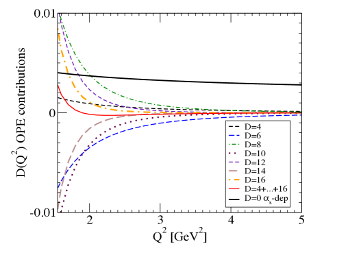
Figure 1: $ud$ V channel $\alpha_{s}$-dependent $D=0$ and non-perturbative $D=4,\cdots,16$ OPE contributions to $D(Q^{2})$, using $\alpha_{s}$ and central $C_{D>4}$ value input described in the text. The $D=0$ curve shows the sum of the $\alpha_{s}$-dependent $D=0$ contributions only, with the $\alpha_{s}$-independent parton-model contribution removed.

These points are illustrated in Figure 1. The figure shows the $D=4$ through $16$ contributions to $D(Q^{2})$, obtained using the central $C_{D}$ values of case (iii) above, together with their much more weakly $Q^{2}$-dependent sum. The $Q^{2}$ range displayed extends down to $1.55\ {\rm GeV}^{2}$, the lower edge of the fit window of Refs. Shintani:2008ga ; Shintani:2010ph . Also shown, for comparison, is the $\alpha_{s}$-dependent part of the 5-loop-truncated perturbative ($D=0$) contribution, evaluated, for definiteness, using the fixed-scale expansion form with 3-flavor $\alpha_{s}$ corresponding to the central 5-flavor PDG result, $\alpha_{s}(M_{Z})=0.1181$. It is evident that no single condensate dominates the $D=4$ through $D=16$ sum for any of the $Q^{2}$ shown, and that there is no evidence of any convergence with dimension in the low-$Q^{2}$ region. (The upturn of the $D=4$ through $D=16$ sum with $Q^{2}$ at the lowest $Q^{2}$ shown is thus an artifact of the truncation of the series, and has no physical meaning.)

Given this evidence for the lack of convergence with $D$ of the $D\geq 4$ series, and the failure of any single low-dimension condensate to dominate the sum, the only safe approach to using lattice HVP data to fix $\alpha_{s}$ is to work at scales $Q^{2}$ sufficiently large that all $D\geq 4$ contributions are simultaneously small relative to the $\alpha_{s}$-dependent $D=0$ contributions of interest for determining $\alpha_{s}$. Working at lower $Q^{2}$, where FESR results predict dangerous higher-$D$ effects are almost certainly present, and almost certainly not amenable to being fitted and removed, makes unavoidable a potentially significant theoretical systematic uncertainty impossible to successfully quantify using lattice data alone. We deal with this issue by using FESR results to identify $Q^{2}$ sufficiently large that all of the estimated individual $D\geq 4$ non-perturbative contributions to $D(Q^{2})$ are safely small, and restrict our analysis to $Q_{1}^{2}$ and $Q^{2}$ lying in this region. Scales above $\sim 3$ to $3.5\ {\rm GeV}^{2}$ appear sufficient for this purpose.

III The lattice HVP

	coarse			fine			superfine
extent	$24^{3}\times 64\times 32$			$32^{3}\times 64\times 32$			$32^{3}\times 64\times 32$
$a^{-1}$ (GeV)	1.7848(50)			2.3833(86)			3.148(17)
$am_{l}$	0.005	0.01	0.02	0.004	0.006	0.008	0.0047
$m_{\pi}$ (GeV)	0.33	0.42	0.54	0.28	0.33	0.38	0.37
measurements	685	110	109	510	352	80	920
$am_{\rm res}$	0.003076(58)			0.0006643(82)			0.0006296(58)
$Z_{V}$	0.71408(58)			0.74404(181)			0.77700(8)

Table 1: Simulation parameters for the ensembles used in this study. $a^{-1}$ and $Z_{V}$ have been measured in Blum:2014tka .

In this work we will use $n_{f}=2+1$ dynamical Domain Wall fermion (DWF) configurations generated by the RBC/UKQCD collaborations and extensively detailed in Refs. Arthur:2012yc ; Blum:2014tka . The relevant ensemble parameters are listed in Tab. 1. Since we work at the high scales suggested by the FESR analysis of the previous section, where the D=2 series and higher terms in the OPE will be negligible, we expect to be able to safely average the results for $\alpha_{s}$ obtained from ensembles with different masses. We have checked that these results are, indeed, consistent within one-sigma errors at the momentum scales used here.

III.1 Lattice computation

We start by considering the lattice analog of the continuum HVP of Eq. 3 with flavour $ud$ content.

One can define a conserved vector current in the DWF discretisation Kaplan:1992bt ; Furman:1994ky with finite fifth dimension extension $L_{s}$, via

$$\mathcal{V}_{\mu}(x) = \sum_{s=1}^{L_{s}}\frac{1}{2}\bigg{(}\bar{\psi}(x+a\hat{\mu},s)\left(1+\gamma_{\mu}\right)U_{\mu}^{\dagger}\left(x+a\frac{\hat{\mu}}{2}\right)\psi(x,s)$$ (10)

$$\qquad-\bar{\psi}(x,s)\left(1-\gamma_{\mu}\right)U_{\mu}\left(x+a\frac{\hat{\mu}}{2}\right)\psi(x+a\hat{\mu},s)\bigg{)},$$

where $U$ is an $SU(3)$ link matrix. We consider the two-point function involving the product of this conserved current and the local vector current $V_{\nu}(x)=Z_{V}\psi(x)\gamma_{\nu}\psi(x)$. This combination has been shown to have no contact term Shintani:2008ga ; Shintani:2010ph ; Boyle:2011hu .

We find it natural to use the definition of lattice momentum that satisfies the lattice Ward identity Karsten:1980wd ,

$$\sum_{\mu}a\hat{Q}_{\mu}e^{iaQ_{\mu}/2}\Pi_{\mu\nu}(Q)=0,\quad a\hat{Q}_{\mu}=2\sin(aQ_{\mu}/2),$$ (11)

where $Q_{\mu}=\frac{2\pi n_{\mu}}{L_{\mu}}$, with $n_{\mu}=[-\frac{L_{\mu}}{2a},\dots,0,\dots,\frac{L_{\mu}}{2a}-1]$ denoting the Fourier modes, and $L_{\mu}$ is the lattice extent in the $\mu$ direction.

III.2 Projection and cylinder cut

The Lorentz structure of the lattice two-point function should be equivalent to that of the continuum version, Eq. (4), up to lattice artifacts from the action and from the breaking of rotational symmetry $O(4)$ under the discrete hyper-cubic group $H_{4}$. Including such artifacts, the lattice two-point function is expected to take the form Shintani:2008ga ; Shintani:2010ph ,

$$\Pi_{\mu\nu}(\hat{Q}:a^{2})=\Pi_{\mu\nu}(\hat{Q})+\sum_{n,m:n+m\geq 2}C_{nm}a^{n+m}\hat{Q}_{\mu}^{n}\hat{Q}_{\nu}^{m}+\sum_{n=1}C_{n}\delta_{\mu\nu}(a^{2}\hat{Q}^{2})^{n}$$ (12)

To limit the impact of lattice artifacts, we utilize momentum reflections when projecting out the transverse piece, $\Pi$:

$$\Pi(\hat{Q}^{2})=\frac{1}{12}\sum_{\mu}\sum_{\nu\neq\mu}\frac{\Pi_{\mu\nu}(\hat{Q})-\Pi_{\mu\nu}(r_{\mu}\hat{Q})}{2\hat{Q}_{\mu}\hat{Q}_{\nu}},$$ (13)

where $r_{\mu}$ is a reflection operator for $Q_{\mu}$ in the $\mu$ direction, $r_{\mu}Q_{\mu}=-Q_{\mu}$. By design, this removes all $(n+m)$-even combinations of hypercubic artifact terms from $\Pi$.

In addition, to further minimize $O(4)$-breaking effects, we perform the reflection projection on purely off-axis, non-zero momenta that have been filtered by a cylinder cut procedure Leinweber:1998im . We accept only momenta lying within a radius ($aw$) of a body-diagonal vector, $n_{\mu}$, with norm $1$, $n_{\mu}=(\pm 1,\pm 1,\pm 1,\pm 1)/2$, explicitly:  PhysRevD.63.094504 ,

$$|aQ_{\mu}-(aQ\cdot n)n_{\mu}|<aw\frac{2\pi}{L}.$$ (14)

By performing the cylinder cut before we convert our momenta to physical units we obtain a consistent physical radius. We find that a very narrow cylinder width, $aw=0.24$, gives smooth results with very limited hyper-cubic artifacts while still providing plenty of data points to use in performing fits, as can be seen in Fig. 2.

III.3 Modelling cut-off effects

We will be attempting to fit the $n_{f}=3$ series for $\Delta$ (Eq. 9) to our lattice data. In principle this fit would involve only one parameter, $\alpha_{s}(\mu)$, if our lattice ensembles were very close to the continuum limit, $a^{2}\rightarrow 0$. With the ensembles available, dictated by current lattice technology, we must, however, also fit residual lattice-spacing artifacts.

Considering the fact that we have projected out several combinations of the possible discretisation effects, and have limited the magnitude of the surviving $O(4)$-breaking terms, we postulate that the momentum-dependent lattice corrections will be the rotation-preserving terms $C_{1}\;a^{2}\hat{Q}^{2}$ and $C_{2}\;(a^{2}\hat{Q}^{2})^{2}$. Such effects, if present in our data, will be evident through linear and quadratic dependences on $\hat{Q}^{2}$. In principle, even higher-order corrections could be present. The data quality, however, does not permit us to identify and fit an additional $(a^{2}\hat{Q}^{2})^{3}$ term.

Another possible cut-off effect in our data, which we will fit and remove, is a correction to the continuum coupling itself,

$$\frac{\alpha_{s}(\mu:a^{2})}{\pi}=\frac{\alpha_{s}(\mu)}{\pi}\left(1+C_{\alpha}a^{2}\right).$$ (15)

Collecting all these correction terms, our fit to $\Delta$ is performed using the fit form

$$\Delta\left(Q_{1}^{2},Q^{2},\mu^{2},\frac{\alpha_{s}(\mu:a^{2})}{\pi}\right)+C_{1}\frac{\left(a^{2}\hat{Q}_{1}^{2}-a^{2}\hat{Q}^{2}\right)}{t_{1}-t}+\,C_{2}\frac{\left((a^{2}\hat{Q}_{1}^{2})^{2}-(a^{2}\hat{Q}^{2})^{2}\right)}{t_{1}-t},$$ (16)

where $\Delta\left(Q_{1}^{2},Q_{2}^{2},\mu^{2},\frac{\alpha_{s}(\mu:a^{2})}{\pi}\right)$ is the continuum perturbative expression for $\Delta$ (Eq. 9), with lattice correction to the coupling. We will choose several subtraction points, $\hat{Q}_{1}^{2}$, and fit our data over a range of $\hat{Q}^{2}>\hat{Q}_{1}^{2}$. We fit both the coupling and all of the correction terms simultaneously. Our final fit thus has only four-parameters: $\alpha_{s}(\mu),\,C_{1},\,C_{2}$ and $C_{\alpha}$.

IV Results

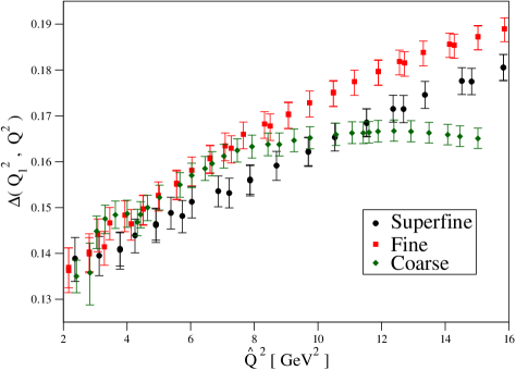
Figure 2: Plot of our results for the quantity $\Delta$ against $\hat{Q}^{2}$ with $\hat{Q}_{1}^{2}$ values from Tab. 2.

We first consider fitting our data using a single renormalisation scale $\mu$. We will find that the single-scale approach produces a large, unphysical, dependence of $\alpha_{s}$ on the scale $\mu$, and fix this problem using an alternate multiple-scale approach. Throughout this section all errors come from the bootstrap.

Fig. 2 illustrates the quality of our data for the quantity $\Delta$ once the reflection projection and cylinder cut procedures have been applied. It is evident that a large linearly-rising behaviour in $\hat{Q}^{2}$ remains for all ensembles and that higher-order effects become significant for the coarse ensemble, and, to a lesser extent, for the fine ensemble data, at large $\hat{Q}^{2}$.

Throughout this work we will perform what is commonly called an “uncorrelated” or weighted fit to our data since we could not find suitable fit ranges where correlated fits were possible. This means that, while remaining a useful metric for goodness of fit, the nominal $\chi^{2}/dof$ should not be taken as having the usual statistical interpretation it would have for a correlated fit. A nominal $\chi^{2}/dof$ of order 1 or greater will, however, indicate a poor fit to our data.

IV.1 Single-scale analysis

We choose to work with the representative fit-ranges shown in Tab. 2. For now, we are forced to use somewhat lower than ideal values of $\hat{Q}_{1}^{2}$ to accommodate the coarse ensemble. This is to ensure the subtraction point $\hat{Q}_{1}^{2}$ is small enough that cut-off effects will be small at $\hat{Q}_{1}^{2}$, allowing us to fit the cut-off effects associated with the higher scale $\hat{Q}^{2}$ using their $\hat{Q}^{2}$ dependence. We also aim to choose subtraction points $\hat{Q}_{1}^{2}$ which are similar for all the ensembles, subject to the constraint that the $\hat{Q}_{1}^{2}$ for each corresponds to a Fourier mode.

ensemble	$\hat{Q}_{1}^{2}$ $[\text{GeV}^{2}]$	$\hat{Q}^{2}$ range $[\text{GeV}^{2}]$
superfine	2.65	$3.78\rightarrow 14.83$
fine	2.44	$3.94\rightarrow 9.74$
coarse	2.68	$3.63\rightarrow 5.02$

Table 2: Fit range parameters for the single-scale and multiple-scale investigations. The specific values relate to particular Fourier modes in the data accessible after the cylinder cut.

In Fig. 3 we show the $\mu$-dependence of our single-scale analysis results for $\alpha_{s}(M_{Z})$. Since the fit range is fixed, and the residual, truncation-induced $\mu$-dependence is small in the continuum limit, the results should be essentially independent of $\mu$ if the single-scale analysis has been successful in bringing the artifacts under control.

What we see instead from Fig. 3 is that the single-scale approach, when applied to our data, produces results with a large-$\mu$ dependence. The $\mu$-dependence is, moreover, much greater than the residual $\mu$-dependence that exists in the continuum truncated perturbative expression.

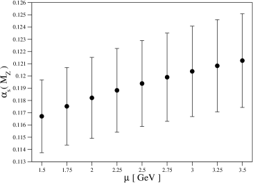
Figure 3: $\mu$-dependence of $\alpha_{s}(M_{Z})$ from the single-scale approach.

All of the fits underlying the results of Fig. 3 have a nominal $\chi^{2}/dof<1$, so it is not that the fits do not describe the data well. Rather the fits lack sufficient information to successfully differentiate between the effects of the continuum coupling and the artifact terms. Similar unphysical $\mu$-dependence is also observed for one or more of the artifact coefficients.

One might think that the results of Fig. 3 are more or less consistent within error, but this is not true, given the very strong correlation among the data points.

IV.2 The multiple-scale analysis

The strong $\mu$ dependence of the single-scale analysis seen in Fig. 3 is clearly unphysical. A good quality fit in a single-scale analysis of our data is thus insufficient to allow both the continuum coupling $\alpha_{s}(\mu)$ and the artifact parameters to be reliably constrained. The fact that the unphysical $\mu$ dependence is large, however, indicates that it must be possible to further constrain the analysis using the known smallness of the residual scale dependence of the five-loop-truncated continuum $D=0$ series.

We thus extend the analysis to perform fits using multiple renormalisation scales $m$. These are run to a common renormalisation scale $\mu$ using the continuum expression of Eq. 2. We use the values $m=2.0,\,2.25,\,2.5$ and $2.75$ GeV for the alternative scale, and for this analysis will vary the renormalisation scale $\mu$ between $1.5$ and $3.5$ GeV as we did for the single-scale analysis for comparison. We will also use the same fit ranges and subtraction points as the single-scale analysis above.

We investigate whether our simultaneous multiple-scale fitting fixes the spurious $\mu$-dependence observed in the single-scale analysis results by again running the coupling to the common five-flavour scale $M_{Z}$. The multiple-scale results for $\alpha_{s}(M_{Z})$ is shown in Fig. 4, for a typical choice of fit ranges.

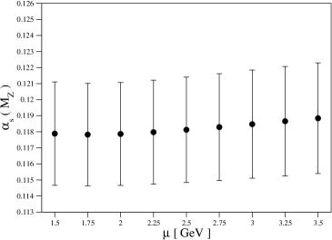
Figure 4: $\mu$-dependence of $\alpha_{s}(M_{Z})$ from the multi-scale approach

If we compare Figs. 3 and 4, we see that indeed the multiple-scale analysis strongly reduces the unphysical $\mu$ dependence of the coupling. This is also the case for all of the artifact parameters, indicating that the lattice artifacts have now been brought under good control over a wide range of scales.

IV.3 Eliminating the coarse data

As seen in Fig. 2, the results from the coarse ensemble have the strongest lattice artifacts. Moreover, to safely fit the data only a small window in $\hat{Q}^{2}$ is suitable. If we consider the same set of $\hat{Q}_{1}^{2}$ as before (Tab. 2) and compare the results of the multi-scale fit using just the superfine and fine ensemble data to those of the corresponding fit using all three ensembles, we see, by varying the upper bound of the coarse-ensemble’s $\hat{Q}^{2}$ fit window, that the coarse ensemble contributes little to the overall fit apart from marginally increasing the statistical uncertainty in the region where the result is stable. This is illustrated in Fig. 5.

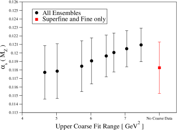
Figure 5: Plot of our value of $\alpha_{s}(M_{Z})$ versus the upper bound in $\hat{Q}^{2}$ of the coarse ensemble fit window, with fixed lower bound, in comparison to the result obtained with the coarse ensemble data entirely removed from the fit.

As Fig. 5 shows, in the (small) fit window for the coarse ensemble (with the superfine and fine fit windows fixed), in the region where the fit appears to be stable the result is consistent with the result of the fit using only superfine and fine data but has slightly larger errors. We conclude that cut-off effects for the coarse ensemble are too large to make employing this ensemble useful for this study. We thus eliminate the coarse ensemble from our fits, and base our final results on fits involving only the superfine and fine data.

IV.4 Multiple $\hat{Q}_{1}^{2}$ choices

ensemble	$\hat{Q}_{1}^{2}$ $[\text{GeV}^{2}]$	Lower $\hat{Q}^{2}$ range $[\text{GeV}^{2}]$	Upper $\hat{Q}^{2}$ range $[\text{GeV}^{2}]$
superfine	3.78,4.25,4.9	$5.5\rightarrow 6.5$	$(2\ {\text{GeV}}^{2}+\text{fine upper bound})\rightarrow 16\ \text{GeV}^{2}$
fine	3.94,4.51,4.99	$5.5\rightarrow 6.5$	$(2\ {\text{GeV}}^{2}+\text{lower\ bound})\rightarrow\ 11\ \text{GeV}^{2}$

Table 3: Fit ranges and subtraction points $\hat{Q}_{1}^{2}$ investigated in the multiple-$\mu$ analyses. Results for the coupling from these varied fit ranges are given in Fig. 6.

Now that we know we can safely omit coarse ensemble data, the much larger cut-off scales of the superfine and fine ensembles make it possible to choose $\hat{Q}_{1}^{2}$ in the range where FESR results indicate the neglect of $D\geq 4$ contributions should be very safe without incurring overly large discretisation effects. For our final results, we perform a multiple-scale analysis with multiple $\hat{Q}_{1}^{2}$ choices to further constrain our fits.

We investigate the fit ranges in Tab. 3 to understand our fit-range dependence. We vary the lower edge of the fit range in steps of $0.5\text{ GeV}^{2}$ and the upper edge of the fit range in steps of $1\text{ GeV}^{2}$. We find good stability when varying the lower bound over this range, keeping the upper fit bound fixed, for the fine and superfine ensembles. In general, it is beneficial to have a low fit bound as close to $\hat{Q}_{1}^{2}$ as possible as this reduces the contributions of the terms proportional to $C_{1}$ and $C_{2}$, and allows the fit to constrain the coupling better.

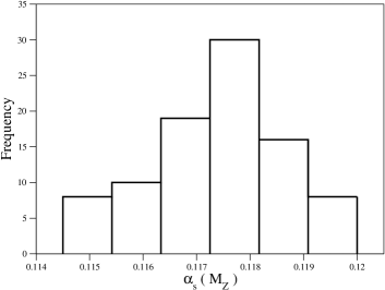
Figure 6: Histogram of the fit-range-dependence of our final result for $\alpha_{s}(M_{Z})$. Results were obtained from a scan over the reasonable fit windows in $\hat{Q}^{2}$ noted in the text.

A histogram of the central values obtained for $\alpha_{s}(M_{Z})$ from a scan over these fit ranges is shown in Fig. 6. We see that some fit-range-dependence does remain, and this will need to be incorporated in our systematic error estimate. Since the distribution is skewed, the systematic error will be asymmetric.

Our central result, corresponding to the maximum of the histogram, is given by the $\hat{Q}^{2}$ fit bounds of $6.04\text{ GeV}^{2}\rightarrow 9.74\text{ GeV}^{2}$ for the fine data and $6.03\text{ GeV}^{2}\rightarrow 14.83\text{ GeV}^{2}$ for the superfine. We use the reference scale $\mu=2\text{ GeV}$.

For these fit ranges, we obtain the following fit parameter results,

$$\begin{gathered}\alpha_{s}(\mu=2\text{ GeV})=0.2961(185),\\ C_{\alpha}=-3.97(36)\text{ GeV}^{2},\quad C_{1}=0.2287(57),\quad C_{2}=-0.0371(16).\end{gathered}$$ (17)

This fit has a nominal $\chi^{2}/dof=0.7(1)$.

IV.5 Error budget

We have identified several sources of systematic uncertainty and have tabulated their effects in Tab. 4. A more in-depth discussion of how these entries were estimated can be found in the following subsections.

Systematic	Estimate
fit range	+0.5%	-1.8%
lattice spacing error	+0%	-0.03%
perturbative truncation	negligible
higher order lattice artifacts	+0.4%	-0.4%

Table 4: Systematic error budget on our final five-flavor result $\alpha_{s}(M_{Z})$

IV.5.1 Fit range

Even though we have tamed the unphysical $\mu$-dependence of the single-scale approach by working at multiple scales, we still see some dependence on our fit ranges, as shown in Fig. 6. All of these results correspond to reasonable fit ranges in $\hat{Q}^{2}$ and a low nominal $\chi^{2}/dof$. To estimate this systematic we will take the one-$\sigma$ deviation of the histogram.

IV.5.2 Lattice spacing error

We cannot propagate the measured distributions for the lattice spacing directly, so we estimate the the impact of the error on the lattice spacing on our final result as a systematic. We do this by introducing $a^{2}$ fit parameters for the fine and superfine ensembles into the final fit with a prior width of the errors given in Tab. 1. This introduces a negligible downward correction to the central value of $\alpha_{s}(M_{Z})$ of the order of 0.03%.

IV.5.3 Perturbative truncation

If we vary the loop order in our analysis, using an estimated value of $d_{5}=400$ to extend this to six loops (in this case, still using just the combination of 4-loop running and 3-loop threshold matching ), we see that our results at three-loop order are consistent with those at six-loop order. Perturbative truncation is thus not a significant source of systematic uncertainty.

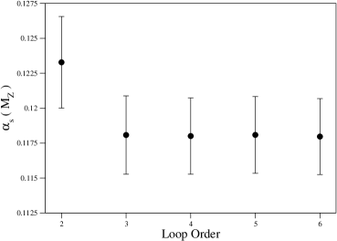
Figure 7: Results for $\alpha_{s}(M_{Z})$ with different orders of truncation for the $D^{(0)}$ series, running and threshold matching An estimate of the unknown parameter $d_{5}$ of 400 was used for the six-loop evaluation.

IV.5.4 Higher order lattice artifacts

With our fit parameters (Eq. 17), we note that the $O(a^{2})$ correction term in $\alpha_{s}(\mu)$ is large even for our superfine ensemble. We found we could not stably fit an $O(a^{4})$ correction term to our data so we must estimate its possible effect. We note that $C_{2}\simeq 0.16\,C_{1}$ and thus expect neglected, higher-order rotation-breaking and rotation-preserving contributions to be smaller than those included in our fits. This is to be expected from the lack of strong curvature in the fine and superfine data of Fig.2 within our chosen fit range.

To estimate the effects of an $a^{4}$ correction on the coupling $\alpha_{s}(\mu)$ we put a coefficient of $a^{4}$ into the fit, with a fixed coefficient of $\pm 1$. Considering the hierarchy represented by the ratio $C_{2}/C_{1}$, we believe this to be a reasonably conservative estimate. Studies with more and finer lattice spacings would be required to further test this assumption. The inserted correction term produces small shifts to the central result of $\alpha_{s}(M_{Z})$ of $\pm 0.4\%$.

IV.6 Result at $M_{Z}$

Our final result for the five-flavor coupling, $\alpha_{s}(M_{Z})$, is

$$\alpha_{s}(M_{Z})=0.1181(27)^{+8}_{-22},$$ (18)

where the first error is statistical and the second contains the systematic errors identified in the previous section combined in quadrature.

V Conclusions

We have revisited the determination of $\alpha_{s}$ from OPE fits to lattice data for the flavor $ud$ vector current HVP, identifying and dealing with several sources of systematic error not recognized in previous implementations of this approach.

One key problem, of particular relevance to low-scale versions of this analysis, is the possibility that multiple numerically significant higher dimension OPE contributions can, through cancellation, produce a sum which mimics lower dimension contributions and hence potentially contaminates the determination of $\alpha_{s}$. Such effects, if present, cannot be fitted and removed using lattice data at Euclidean $Q^{2}$ alone. Continuum FESR results were (i) shown to confirm that this problem was almost certainly present at the low scales, $Q^{2}<3\ \text{GeV}^{2}$, of the previous versions of this analysis, then (ii) used further to identify those $Q^{2}$ at which all such higher dimension OPE contributions should be safely negligible. For such $Q^{2}$, the lattice HVP should be dominated by dimension $0$ (perturbative) OPE contributions and residual lattice artifact contributions, with the latter to be fitted and removed. We have introduced a momentum-reflection-based projection method for the lattice HVP and employed a very narrow cylinder cut to further reduce higher-order rotation-breaking cut-off effects.

A second key problem is the large, unphysical, $\mu$ dependence observed when employing the (previously used) single-scale approach to fitting the HVP data. This problem was rectified by implementing a multiple-scale analysis strategy.

We find that some residual fit-range dependence does remain, even after performing a multiple-scale, multiple-$Q_{1}^{2}$ analysis. For the lattice spacings of the present study, lattice artifacts are not small in the $Q^{2}$ range employed and these had to be carefully modelled to obtain a well-behaved result. Additional ensembles finer than the superfine ensemble employed here (which will have smaller lattice artifacts in the same $Q^{2}$ range) should help to further reduce the systematic uncertainty, as well as improve statistics. One significant advantage of our approach is that simulations at multiple unphysical (heavy) pion masses can be used simultaneously and averaged to improve statistics, since, for the $Q^{2}$ in our chosen fit windows, mass-dependent OPE contributions are negligible over the range of $m_{\pi}$ typical of modern simulations.

Our final result is consistent with both the PDG central value of $0.1181(11)$ Olive:2016xmw and the FLAG result of $0.1182(12)$ Aoki:2016frl . Our errors, both statistical and systematic, are currently larger, but checking for consistency is important for the determination of such a fundamental constant. We also believe we have identified the source of the tension between the world average and the results of the previous, lower-scale version of this analysis Shintani:2010ph (which gave $\alpha(M_{Z})=0.1118^{+16}_{-17}$) and, with our improved method, have succeeded in solving the problems that led to this tension. Future improvements to both the statistical and systematic errors, moreover, appear technically straightforward.

We conclude by stressing the close relation of the lattice HVP approach discussed in this paper to the $\tau$-decay-data-based FESR determination of $\alpha_{s}$. Both involve an analysis of the same object, the flavor $ud$ HVP. The lattice approach, however, has certain important advantages. In particular, while the somewhat low scale of the $\tau$ mass makes unavoidable the presence of higher dimension OPE and DV contributions in the FESR analysis, DV contributions are exponentially suppressed at the Euclidean $Q^{2}$ of the lattice analysis and, with modern lattices, it is feasible to work at scales, $Q^{2}$, where higher dimension OPE contributions are safely negligible. The price to pay for these advantages is the presence of residual lattice artifacts that have to be fit and removed from the lattice HVP data at these higher scales. This procedure, however, is subject to systematic improvement through increased statistics and the use of finer lattices with reduced artifact contributions. As such, it appears to us that, in the long run, the lattice approach represents the more favourable of the two methods for extracting $\alpha_{s}$ from the light-quark HVP.

VI Acknowledgements

This work was supported by the DiRAC Blue Gene Q Shared Petaflop system at the University of Edinburgh, operated by the Edinburgh Parallel Computing Centre on behalf of the STFC DiRAC HPC Facility (www.dirac.ac.uk). This equipment was funded by BIS National E-infrastructure capital grant ST/K000411/1, STFC capital grant ST/H008845/1, and STFC DiRAC Operations grants ST/K005804/1 and ST/K005790/1. We would thank to the members of RBC/UKQCD collaboration for helpful discussions and comments. RJH, RL and KM are sponsored by the Natural Sciences and Engineering Research Council of Canada (NSERC). ES is grateful to RIKEN Advanced Center for Computing and Communication (ACCC) and the Mainz Institute for Theoretical Physics (MITP).

VII Appendices

Here we put the relevant series coefficients for the perturbative series we have used in this work. All coefficients are for the $n_{f}=3$ variants.

VII.1 $\beta$-function coefficients

$$\beta_{0}=9/4,\quad\beta_{1}=4,\quad\beta_{2}=3863/384,\quad\beta_{3}=47.228040.$$ (19)

VII.2 Running coupling expansion coefficients

$$\begin{gathered}A_{21}=-\beta_{0},\\ A_{32}=\beta_{0}^{2},\quad A_{31}=-\beta_{1},\\ A_{43}=-\beta_{0}^{3},\quad A_{42}=\frac{5}{2}\beta_{0}\beta_{1},\quad A_{41}=-\beta_{2},\\ A_{54}=\beta_{0}^{4},\quad A_{53}=-\frac{13}{3}\beta_{0}^{2}\beta_{1},\quad A_{52}=\frac{3\beta_{1}^{2}+6\beta_{0}\beta_{2}}{2},\quad A_{51}=-\beta_{3}.\end{gathered}$$ (20)

VII.3 $D^{(0)}$ series coefficients

$$\begin{gathered}d_{00}=1,\quad d_{10}=1,\\ d_{20}=1.639821,\quad d_{21}=-2.25,\\ d_{30}=6.371014,\quad d_{31}=-11.379195,\quad d_{32}=5.0625,\\ d_{40}=49.075700,\quad d_{41}=-66.182813,\\ \quad d_{42}=47.404784,\quad d_{43}=-11.390625,\\ d_{50}=d_{5},\quad d_{51}=-598.354375,\quad d_{52}=388.732597,\\ \quad d_{53}=-162.464353,\quad d_{54}=25.628906.\end{gathered}$$ (21)

References

- (1) LHC Higgs Cross Section Working Group, J.R. Andersen et al., (2013), arXiv:1307.1347.
- (2) C. Anastasiou et al., JHEP 16 (2016) 058, arXiv:1602.00695.
- (3) M.E. Peskin, Proceedings, 2013 Community Summer Study on the Future of U.S. Particle Physics: Snowmass on the Mississippi (CSS2013): Minneapolis, MN, USA, July 29-August 6, 2013, 2013, arXiv:1312.4974.
- (4) G.P. Lepage, P.B. Mackenzie and M.E. Peskin, (2014), arXiv:1404.0319.
- (5) S. Aoki et al., Eur. Phys. J. C77 (2017) 112, arXiv:1607.00299.
- (6) Particle Data Group, C. Patrignani et al., Chin. Phys. C40 (2016) 100001.
- (7) ETM, B. Blossier et al., Phys. Rev. D89 (2014) 014507, arXiv:1310.3763.
- (8) A. Bazavov et al., Phys. Rev. D90 (2014) 074038, arXiv:1407.8437.
- (9) B. Chakraborty et al., Phys. Rev. D91 (2015) 054508, arXiv:1408.4169.
- (10) Y. Maezawa and P. Petreczky, Phys. Rev. D94 (2016) 034507, arXiv:1606.08798.
- (11) M. Luscher et al., Nucl. Phys. B413 (1994) 481, hep-lat/9309005.
- (12) ALPHA, M. Bruno et al., Phys. Rev. Lett. 119 (2017) 102001, 1706.03821.
- (13) Z. Fodor et al., JHEP 11 (2012) 007, arXiv:1208.1051.
- (14) M. Beneke and M. Jamin, JHEP 09 (2008) 044, arXiv:0806.3156.
- (15) K. Maltman and T. Yavin, Phys. Rev. D78 (2008) 094020, arXiv:0807.0650.
- (16) D. Boito et al., Phys. Rev. D85 (2012) 093015, arXiv:1203.3146.
- (17) D. Boito et al., Phys. Rev. D91 (2015) 034003, arXiv:1410.3528.
- (18) A. Pich and A. Rodríguez-Sánchez, Phys. Rev. D94 (2016) 034027, arXiv:1605.06830.
- (19) D. Boito et al., Phys. Rev. D95 (2017) 034024, arXiv:1611.03457.
- (20) TWQCD, JLQCD, E. Shintani et al., Phys. Rev. D79 (2009) 074510, arXiv:0807.0556.
- (21) E. Shintani et al., Phys. Rev. D82 (2010) 074505, arXiv:1002.0371, [Erratum: Phys. Rev.D89,no.9,099903(2014)].
- (22) P.A. Baikov, K.G. Chetyrkin and J.H. Kuhn, Phys. Rev. Lett. 118 (2017) 082002, arXiv:1606.08659.
- (23) T. van Ritbergen, J. Vermaseren and S. Larin, Phys. Lett. B400 (1997) 379, hep-ph/9701390.
- (24) K.G. Chetyrkin, J.H. Kuhn and C. Sturm, Nucl. Phys. B744 (2006) 121, hep-ph/0512060.
- (25) K.G. Chetyrkin and A. Kwiatkowski, Z. Phys. C59 (1993) 525, hep-ph/9805232.
- (26) R.J. Hudspith et al., (2017), arXiv:1702.01767.
- (27) P.A. Baikov, K.G. Chetyrkin and J.H. Kühn, Phys. Rev. Lett. 101 (2008) 012002, arXiv:0801.1821.
- (28) L.R. Surguladze and M.A. Samuel, Phys. Rev. Lett. 66 (1991) 560, [Erratum: Phys. Rev. Lett.66,2416(1991)].
- (29) S.G. Gorishnii, A.L. Kataev and S.A. Larin, Phys. Lett. B259 (1991) 144.
- (30) K.G. Chetyrkin, A.L. Kataev and F.V. Tkachov, Phys. Lett. B85 (1979) 277.
- (31) RBC, UKQCD, T. Blum et al., Phys. Rev. D93 (2016) 074505, arXiv:1411.7017.
- (32) RBC, UKQCD, R. Arthur et al., Phys. Rev. D87 (2013) 094514, arXiv:1208.4412.
- (33) D.B. Kaplan, Phys. Lett. B288 (1992) 342, hep-lat/9206013.
- (34) V. Furman and Y. Shamir, Nucl. Phys. B439 (1995) 54, hep-lat/9405004.
- (35) P. Boyle et al., Phys. Rev. D85 (2012) 074504, arXiv:1107.1497.
- (36) L.H. Karsten and J. Smit, Nucl. Phys. B183 (1981) 103, [,495(1980)].
- (37) UKQCD collaboration, D.B. Leinweber et al., Phys. Rev. D58 (1998) 031501, hep-lat/9803015.
- (38) C. Alexandrou, P. de Forcrand and E. Follana, Phys. Rev. D 63 (2001) 094504.