Polarization of spontaneous magnetic field and magnetic fluctuations in $s+is$ anisotropic multiband superconductors

Abstract

We show that multiband superconductors with broken time-reversal symmetry can produce spontaneous currents and magnetic fields in response to the local variations of pairing constants. Considering the iron pnictide superconductor Ba_1-xK_xFe₂As₂ as an example we demonstrate that both the point-group symmetric $s+is$ state and the C₄-symmetry breaking $s+id$ states produce in general the same magnitudes of spontaneous magnetic fields. In the $s+is$ state these fields are polarized mainly in ab crystal plane, while in the $s+id$ state their ab-plane and c-axis components are of the same order. The same is true for the random magnetic fields which are produced by the order parameter fluctuations near the critical point of the time-reversal symmetry breaking phase transition. Our findings can be used as a direct test of the $s+is/s+id$ dichotomy and the additional discrete symmetry breaking phase transitions with the help of muon spin relaxation experiments.

Introduction. Superconducting states with spontaneously broken time-reversal symmetry (BTRS) have been recently in the focus of interest. First such states have been studied in connection with the chiral p-wave order parameter in the superfluid ³He A phaseVolovik (2009) and Sr₂RuO₄ superconducting compoundMackenzie and Maeno (2003). More recently, $s+id$ and $s+is$ states have been suggested as the candidate order parameters in multiband iron pnictide compoundsLee et al. (2009); Platt et al. (2012); Thomale et al. (2011); Maiti and Chubukov (2013); Carlström et al. (2011); Watanabe et al. (2014); Okazaki et al. (2012). Recent experimentGrinenko et al. (2017) supports this hypothesis demonstrating the presence of spontaneous currents in the ion irradiated samples of Ba_1-xK_xFe₂As₂ in the certain doping level interval.

Spontaneous currents were predicted to exist near impurities in $s+id$ superconducting states which spontaneously break the C₄ crystalline symmetry of the parent compound Lee et al. (2009). As for the $s+is$ states, initially it has been claimed that magnetic field can appear only in samples subjected to strain Maiti et al. (2015). However, this conclusion was made based on the specific circularly-symmetric model of the impurity.

More general consideration has shownSilaev et al. (2015); Garaud et al. (2016) that magnetic fields in the $s+is$ state can be generated without strain in the presence of the general-form inhomogeneities of the order parameter. They can be induced e.g. by the domain wall between $s+is$ and $s-is$ statesGaraud and Babaev (2014), attached to the sample edge or by any external controllable perturbation such as the local heating. Later the particular case of two-dimensional defects elongated along the crystal c-axis and forming square shapes in the ab plane have been studied (Lin et al., 2016). In such system the spontaneous magnetic field generated in $s+is$ state is several order of magnitude smaller than in the $s+id$ one. As we show below this difference is not generic and under more general conditions the magnetic field amplitudes produced in two states are of the same order.

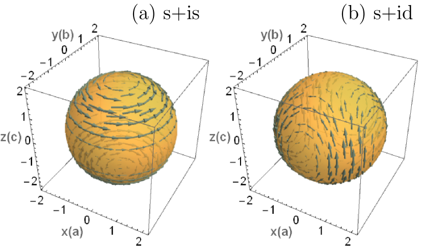
Figure 1: Arrows show the spontaneous magnetic fields generated by rotationally symmetric 3D inhomogeneity of the interband phase difference $\theta_{13}=\theta_{13}(r)$ as given by the Eq.(2). (a) Anisotropic $s+is$ state with $\gamma^{x}_{13}=\gamma^{y}_{13}=2\gamma^{z}_{13}$ and (b) $s+id$ state with $\gamma^{z}_{13}=0$ and $\gamma^{x}_{13}=-\gamma^{y}_{13}$. The scale of magnetic field is the same in (a,b). The field is plotted on the spherical surface $r=const$. The crystal anisotropy axis is $z$. The field is rotationally symmetric in $s+is$ state and changes the sign under the $C_{4}$ rotation in $s+id$ state.

The purpose of the present paper is threefold. First, we show that the spontaneous magnetic field is generated both in the $s+is$ and $s+id$ state due to the general-form inhomogeneities of the pairing interactions. Such form of disorder can exist in the sample even without the externally generated defects just due to the spatially-inhomogeneous doping level. Second, we demonstrate that in the general case, when the system is inhomogeneous both in the ab-plane and in the c-direction $s+is$ and $s+id$ states yield the same magnitudes of spontaneous fields. However, as shown schematically in Fig.(1) this regime is characterized by the qualitatively different polarizations of the spontaneous field in $s+id$ and $s+is$ states. This prediction can be used for resolving the $s+id/s+is$ dichotomy in real materials with the help of muon spin relaxation experimentsSonier et al. (2000); Mahyari et al. (2014); Grinenko et al. (2017). Third, we demonstrate that the order parameter fluctuations near the BTRS phase transition generate random magnetic fields with the critical correlation radius. Thus, the discrete symmetry breaking phase transition can be revealed through the magnetic field fluctuations.

Three-band model. Here we develop general treatment of spontaneous magnetic fields in BTRS states further considering inhomogeneities created by the spatial variation of pairing constants in the minimal three-band microscopic model Stanev and Tešanović (2010); Marciani et al. (2013); Maiti and Chubukov (2013) with three distinct superconducting gaps $\Delta_{1,2,3}$ residing in different bands. The pairing which leads to the BTRS state is dominated by the competition of two interband repulsion channels $\eta_{1,2}>0$ described by the following coupling matrix

$$\hat{\Lambda}=-\nu_{0}\left(\begin{array}[]{ccc}0&\eta_{1}&\eta_{2}\\ \eta_{1}&0&\eta_{2}\\ \eta_{2}&\eta_{2}&0\\ \end{array}\right)\,.$$ (1)

We assume for simplicity that the density of states $\nu_{0}$ is the same in all superconducting bands. This model can be used for both the $s+is$ and $s+id$ states. In the former case $\Delta_{1,2}$ correspond to the gaps at hole pockets and $\Delta_{3}$ is the gap at electron pockets, so that $u_{hh}=\nu_{0}\eta_{1}$ and $u_{eh}=\nu_{0}\eta_{2}$ are respectively the hole-hole and electron-hole interactions Marciani et al. (2013); Maiti and Chubukov (2013). The same model (1) can be used to describe the $s+id$ states but there, $\Delta_{1}$ and $\Delta_{2}$ describe gaps in $(0,\pm\pi)$ and $(\pm\pi,0)$ electron pockets, respectively. In the hole pocket the gap is $\Delta_{3}$, so that $u_{eh}=\nu_{0}\eta_{1}$ and $u_{ee}=\nu_{0}\eta_{2}$ are electron-hole and electron-electron interactions respectively (Garaud et al., 2017, 2016).

The inhomogeneities of pairing interactions in the model (1) produce spatially varying gap amplitudes $|\Delta_{i}|$ and phases $\theta_{i}$. Their gradients can generate spontaneous magnetic field according to the modified London expression in multiband superconductorsSilaev et al. (2015)

$${\bm{B}}=-4\pi\nabla\times\left(\hat{\lambda}^{2}_{L}{\bm{j}}\right)+\frac{1}{\tilde{e}N}\sum_{k>i}\nabla\times\left(\hat{\gamma}_{ki}\nabla\theta_{ki}\right),$$ (2)

where we use the units with $\hbar=c=1$ and introduce interband phases $\theta_{ki}=\theta_{k}-\theta_{i}$. Here the London penetration depth is given by $\hat{\lambda}^{-2}_{L}=\sum_{k}\hat{\lambda}^{-2}_{k}$ and $\hat{\gamma}_{ki}=\hat{\lambda}_{L}^{2}(\hat{\lambda}_{k}^{-2}-\hat{\lambda}_{i}^{-2})$ , where $\hat{\lambda}_{k}$ are in general the tensor coefficients characterizing contribution of each band to the Meissner screening. In the clean limit they can be expressed as follows

$$\hat{\lambda}^{-2}_{k}=8\pi\rho{\tilde{e}}^{2}\hat{K}_{k}|\Delta_{k}|^{2},$$ (3)

where $\hat{K}_{k}=\langle\bm{v}_{k}\bm{v}_{k}\rangle$ is the anisotropy tensor, $\bm{v}_{k}$ is the Fermi velocity in $k$-th band normalized to the certain band-independent characteristic velocity $\bar{v}_{F}$. We normalize the gaps by $T_{c}/\sqrt{\rho}$, where $\rho=\sum_{n}\pi T_{c}^{3}\omega_{n}^{-3}\approx 0.1$ and $T_{c}$ is the critical temperature, magnetic field by $B_{0}=T_{c}\sqrt{\nu_{0}/\rho}$, which is close to the thermodynamic critical field at zero temperatureSaint-James et al. (1970). Length is normalized by the Cooper pair size $\xi_{0}=\bar{v}_{F}/T_{c}$, and we introduce the dimensionless Cooper pair charge is $\tilde{e}=2e\xi_{0}^{2}B_{0}$.

In contrast to the usual London electrodynamics, the multicomponent superconducting systems can generate spontaneous magnetic fields due the second term in Eq.(2) acting as a source according to the mechanisms described below. The source term in Eq.(2) is non-zero if $\nabla\theta_{ki}\neq 0$ and tensors $\hat{\gamma}_{ki}$ are constant in space but anisotropic. This scenario is generic for the $s+id$ state when all three components $\gamma^{x,y,z}_{ki}$ are different. The $s+is$ state is isotropic in ab plane, but there is anisotropy in ca and cb planes $\gamma_{ki}^{x}=\gamma_{ki}^{y}\neq\gamma_{ki}^{z}$. In this case the ab-plane inhomogeneities are decoupled from the magnetic field Lin et al. (2016), so that $B_{z}=0$. However, in general the systems is inhomogeneous along the c-axis direction as well, which yields the magnetic response $B_{x,y}$ of the same magnitude as the $s+id$ state.

The general field structures produced by the 3D inhomogeneity in $s+is/s+id$ states can be found using Eq.(2). In Fig.1 we show spontaneous field produced by the interband phase difference modulation $\theta_{13}(r)$. On the $s+is$ case only $B_{x,y}\neq 0$ while in $s+id$ state the field has all components.

Second, the component $B_{z}\neq 0$ can be generated even in $s+is$ stateGaraud and Babaev (2014); Garaud et al. (2016); Silaev et al. (2015); Lin et al. (2016). According to Eq.(2) for that we need simultaneously $\nabla_{x,y}\theta_{ki}\neq 0$ and $\nabla_{x,y}\gamma^{x,y}_{ki}\neq 0$ with additional requirement that these gradients are non-collinear to each other. Therefore $B_{z}$ component in $s+is$ state is significantly smaller than in the $s+id$ state, where only $\nabla_{x,y}\theta_{ki}\neq 0$ is needed. Therefore the largest spontaneous field in the $s+is$ case appears in the direction perpendicular to the anisotropy axis, while in $s+id$ all components are of the same order. On can distinguish between these states by analysing the polarization of spontaneous magnetic fields with the help of the muon spin relaxation techniquesSonier et al. (2000); Mahyari et al. (2014); Grinenko et al. (2017). Below we illustrate these conclusions using more detailed calculations close to $T_{c}$ using the Ginzburg-Landau (GL) theory.

Ginzburg-Landau calculation. To go beyond local approximation we can calculate spontaneous magnetic fields using GL theory derived for $s+is/s+id$ states Garaud et al. (2017, 2016) corresponding to the model (1). The general free energy density, normalized to $B_{0}^{2}$ is given by $F=F_{s}+B^{2}/8\pi$, where the GL free energy describing both the $s+is$ and $s+id$ states is given by

$$F_{s}=\sum_{j=1}^{2}\left((\bm{\hat{\Pi}}\psi_{j})^{*}\hat{k}_{jj}(\bm{\hat{\Pi}}\psi_{j})+\alpha_{j}|\psi_{j}|^{2}+\frac{\beta_{j}}{2}|\psi_{j}|^{4}\right)$$

$$+2(\bm{\hat{\Pi}}\psi_{1})^{*}\hat{k}_{12}\bm{\hat{\Pi}}\psi_{2}+\gamma|\psi_{1}|^{2}|\psi_{2}|^{2}+\delta\psi_{1}^{*2}\psi_{2}^{2}+c.c,$$ (4)

where $\bm{\hat{\Pi}}=\nabla-i\tilde{e}\bm{A}$. This model is formulated in terms of the two order parameters $\psi_{1}$ and $\psi_{2}$ which are related to the individual gap functions within separate bands as $(\Delta_{1},\Delta_{2},\Delta_{3})=(\zeta\psi_{2}-\psi_{1},\zeta\psi_{2}+\psi_{1},\psi_{2})$, where $\zeta=(\eta_{1}-\sqrt{\eta^{2}_{1}+8\eta^{2}_{2}})/4\eta_{2}$.

The coefficients of gradient terms in Eq.(4) are combined from the anisotropy tensors characterising each superconducting band as follows

$$\hat{k}_{11}=\rho(\hat{K}_{1}+\hat{K}_{2})$$ (5)

$$\hat{k}_{22}=\rho[\zeta^{2}(\hat{K}_{1}+\hat{K}_{2})+\hat{K}_{3}]$$ (6)

$$\hat{k}_{12}=\zeta\rho(\hat{K}_{2}-\hat{K}_{1})$$ (7)

The difference between $s+is$ and $s+id$ symmetries is determined by the structure of mixed-gradient coefficients (7) in ab plane. That is for $s+is$ state $K_{i}^{x}=K_{i}^{y}\equiv K_{i}^{xy}$ so that $k_{12}^{x}=k_{12}^{y}\equiv k_{12}^{xy}$. For $s+id$ state $K_{1,2}^{x}\neq K_{1,2}^{b}$ but $K_{1}^{x}=K_{2}^{y}$ so that $k_{12}^{x}=-k_{12}^{y}\equiv k_{12}^{xy}$. Despite having quite different properties in the ab plane both states are characterized by the anisotropy in ca and cb planes determined by the coefficients $K_{i}^{z}\neq K_{i}^{x},K_{i}^{y}$. In $s+is$ state this anisotropy provides linear coupling between magnetic field and pairing constant inhomogeneities. For that at least two bands should have different anisotropies, otherwise the problem can be rescaled to the fully isotropic one when only the non-linear coupling is possible yielding much smaller spontaneous currents.

$\begin{array}[]{c}\includegraphics[width=433.62pt]{s_plus_isd_lattice_7.png}\end{array}$

Figure 2: (Color online) (a,b) Order parameter modulation produced by the ab-plane inhomogeneities of the form (12). The corresponding spontaneous field $B_{z}$ is shown for (c) $s+is$ state with $K^{xy}_{1}=1$, $K^{xy}_{2}=1.5$, $K^{xy}_{3}=0.5$ and (d) $s+id$ state with $K^{x}_{1}=K^{y}_{2}=1$, $K^{y}_{1}=K^{x}_{2}=1.5$ and $K^{xy}_{3}=0.5$. GL parameter is $\tilde{e}=1/4$ , $\tau=0.2$, the field is normalized to $\tau B_{0}/\tilde{e}$.

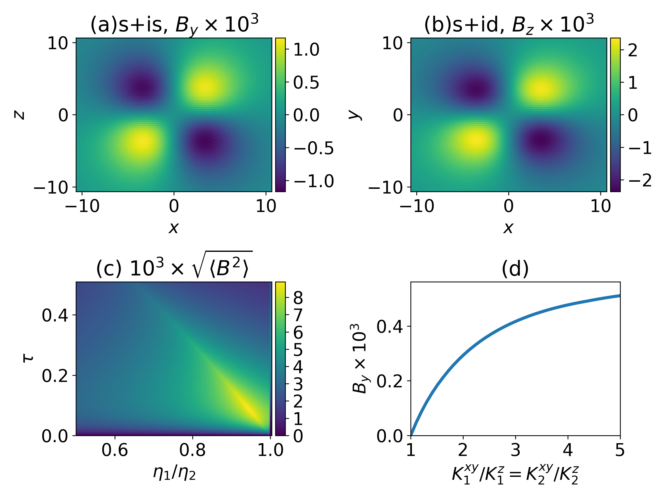
Figure 3: (a,b) Spontaneous fields produced by the inhomogeneities of the pairing constant $\eta_{2}(\bm{r})$ (13,14) and $\eta_{1}=1$. (a) ca-plane defect in $s+is$ superconductor with anisotropy parameters for $s+is$ are $K^{xy}_{1}=1$, $K^{xy}_{2}=1.5$, $K^{xy}_{3}=0.5$, $K^{z}_{1}=2$, $K^{z}_{2}=3$, $K^{z}_{3}=0.5$. (b) ab-plane defects in $s+id$ state characterized by $K^{x}_{1}=K_{2}^{y}=1$, $K^{y}_{1}=K^{x}_{2}=1.5$, $K^{x}_{3}=K^{y}_{3}=0.5$. GL parameter $\tilde{e}=1/4$ for both cases, $\tau=0.2$. The field is normalized to $\tau B_{0}/\tilde{e}$. (c) Spontaneous magnetic field in the ab-plane produced by the critical fluctuations near the BTRS transitions in anisotropic $s+is$ state. The field is measured in $(|k_{12}^{z}-k_{12}^{xy}|/\sqrt{k_{11}k_{22}})(T_{c}/E_{F})B_{0}$, where $E_{F}$ is the Fermi energy. The field maximum at each value of $\eta_{1}/\eta_{2}$ corresponds to the BTRS critical temperature. (d) The magnitude of the in-plane magnetic field vs. the effective mass anisotropy in the $s+is$ superconductors.

The other coefficients in GL expansion (4) are expressed in terms of the pairing constants (1) as

$$\alpha_{1}=-2(G_{0}-G_{1}+\tau)$$ (8)

$$\alpha_{2}=-(1+2\zeta^{2})(G_{0}-G_{2}+\tau)$$ (9)

$$\beta_{1}=2;\;\beta_{2}=1+2\zeta^{4}$$ (10)

$$\gamma=4\zeta^{2};\;\delta=2\zeta^{2}$$ (11)

where $\tau=1-T/T_{c}$, $G_{1}=1/\eta_{1}$ and $G_{2}=\left(\eta_{1}+\sqrt{\eta^{2}_{1}+8\eta^{2}_{2}}\right)/4\eta_{2}^{2}$ are the positive eigenvalues of the matrix (1) $\hat{\Lambda}^{-1}$ and $G_{0}=\min(G_{1},G_{2})$. The Ginzburg-Landau model is valid in the vicinity of $T_{c}$ when both order parameters $|\psi_{1}|$ and $|\psi_{2}|$ are small. In this regime the bulk BTRS state appears for the close values of pairing constants due to the following reason. In the homogeneous state both order parameters appear simultaneously when $\eta_{1}=\eta_{2}$. In case of the finite detuning, one of the order parameters nucleates first. E.g. when $\eta_{1}>\eta_{2}$ the $\psi_{1}$ state nucleates at $T_{c}$ since $G_{0}=G_{1}<G_{2}$. Then the bulk critical temperature of the BTRS transition, that is nucleation of $\psi_{2}$ in this case can be found from the relation $\alpha_{2}=-2\zeta^{2}|\psi_{1}|^{2}$, which is equivalent to $\tau=G_{2}-G_{1}+\zeta^{2}|\psi_{1}|^{2}$. The we have the restriction $|G_{1}-G_{2}|\leq\tau$ so that $|1-\eta_{1}/\eta_{2}|\leq\tau$. The inhomogeneous BTRS state however occurs for much larger amplitudes of the pairing constant variations because the additional order parameter nucleates locally at the regions where $\eta_{1}\approx\eta_{2}$.

Below, we consider the spontaneous magnetic field produced by the superconducting currents generated by the inhomogeneities of the pairing constant $\eta_{2}=\eta_{2}(\bm{r})$. At first let us consider the 2D inhomogeneities in the ab plane, so that $\eta_{1}=1$ and

$$\eta_{2}(x,y)=1+0.5\sin(x/2)\sin(y/2).$$ (12)

This model allows for demonstrating differences between the linear and non-linear mechanisms of the spontaneous current generation, where the former takes place for $s+id$ and the latter is $s+is$ pairings. The magnetic field produced by ab-inhomogeneities has only z-component. The calculated distributionc of $B_{z}=B_{z}(x,y)$ is shown in Figc.2c,d. Where the magnetic field is given in the units of $\tau B_{0}/\tilde{e}$ which has an order of the upper critical field $H_{c2}$ at a given temperature. One can see that for one and the same set of parameters $s+is$ state yields the spontaneous magnetic field response about $10^{2}$ times smaller than $s+id$, which is consistent with the results obtained before Lin et al. (2016).

Except of the special case of ab-plane inhomogeneities, in general the $s+is$ and $s+id$ states produce the magnetic fields of comparable amplitudes. To demonstrate this we compare responses produced by the pairing constant variation given by

$$\eta_{2}=1+0.5e^{-(x^{2}+y^{2})/8} s+id$$ state (13)

$$\eta_{2}=1+0.5e^{-(x^{2}+z^{2})/8} s+is$$ state (14)

The former inhomogeneity (13) corresponds to the ab-plane defect, while the latter (14) is the ca-plane defect. To obtain spontaneous fields produced by ca-plane defects in $s+is$ case we assume that there is ca-plane anisotropy set by the choice of coefficient ratio in different bands $K^{xy}_{1}=1$, $K^{xy}_{2}=1.5$, $K^{xy}_{3}=0.5$, $K^{z}_{1}=2$, $K^{z}_{2}=3$, $K^{z}_{3}=1$. Such system yields the magnetic field component $B_{y}(x,z)$ shown in Fig.3a. One can compare it with the qualitatively similar distribution of $B_{z}$ component produced by the Gaussian ab-plane inhomogeneity (13) in the $s+id$ state shown in Fig.3b. Magnetic signatures of ca-defect in $s+id$ states are qualitatively similar to that in $s+is$ shown in Fig.3a. In ca-plane the $s+id$ state is described by structurally identical GL equations as the $s+is$ one with the interchange $K_{k}^{xy}\to K_{k}^{x}$. The 122 iron pnictide compounds has been shown to feature anisotropy which can vary from in rather wide limits from $K_{i}^{xy}/K_{i}^{z}\approx 1-3$ (Yuan et al., 2009) to $K_{i}^{xy}/K_{i}^{z}\approx 4-5$ Tafti et al. (2014). In Fig.3d we show the field amplitude dependence on the degree of anisotropy $K_{1}^{z}/K_{1}^{xy}=K_{2}^{z}/K_{2}^{xy}\neq 1$ and fixing $K_{3}^{z}/K_{3}^{xy}=1$.

The general analytical expression for spontaneous field in case of the 3D inhomogeneity can be obtained using the reduced GL theory in the vicinity of BTRS transition. It can be constructed assuming the main order parameter to be $\psi_{1}=|\psi_{1}|e^{i\varphi_{1}}$ with $|\psi_{1}|=const$ and introducing the BTRS order parameter $\Theta=-i(\psi_{2}\psi_{1}^{*})/|\psi_{1}|$. Then we represent the GL free energy in terms if the gauge-invariant momentum $\bm{Q}=\bm{A}-\nabla\varphi_{1}/\tilde{e}$, the real and imaginary parts of the complex order parameter $\Theta=\Theta_{r}+i\Theta_{im}$ as follows

$$F(\Theta,\bm{Q})=\tilde{\alpha}_{r}\Theta^{2}_{r}+\tilde{\alpha}_{im}\Theta^{2}_{im}+\frac{\beta_{2}}{2}|\Theta|^{4}+\frac{|\nabla\times\bm{Q}|^{2}}{8\pi}+$$

$$|\psi_{1}|^{2}\tilde{e}^{2}\bm{Q}\hat{k}_{11}\bm{Q}+2|\psi_{1}|\tilde{e}\bm{Q}\hat{k}_{12}\left(\nabla\Theta_{r}+\tilde{e}\bm{Q}\Theta_{im}\right)+$$

$$\left(\nabla+i\tilde{e}\bm{Q}\right)\Theta^{\ast}\hat{k}_{22}\left(\nabla-i\tilde{e}\bm{Q}\right)\Theta.$$ (15)

Here $\tilde{\alpha}_{r}=\alpha_{2}+|\psi_{1}|^{2}(\delta-\gamma)$ and $\tilde{\alpha}_{im}=\alpha_{2}+|\psi_{1}|^{2}(\delta+\gamma)$. Equation $\tilde{\alpha}_{r}(T)=0$ gives the critical temperature of BTRS transition. In the vicinity of this transition only the variation of $\Theta_{r}$ is important as the $\tilde{\alpha}_{im}$ is positive and non-vanishing. Therefore we can describe the time-reversal symmetry breaking phase transition in terms of the real-valued order parameter $\Theta_{r}$:

$$F(\Theta_{r},\bm{Q})=\tilde{e}^{2}|\psi_{1}|^{2}\bm{Q}\hat{k}_{11}\bm{Q}+\tilde{e}^{2}\Theta_{r}^{2}\bm{Q}\hat{k}_{22}\bm{Q}+\frac{|\nabla\times\bm{Q}|^{2}}{8\pi}$$

$$\tilde{\alpha}_{r}\Theta_{r}^{2}+\frac{\beta_{2}}{2}\Theta_{r}^{4}+\nabla\Theta_{r}\hat{k}_{22}\nabla\Theta_{r}+2\tilde{e}|\psi_{1}|\bm{Q}\hat{k}_{12}\nabla\Theta_{r}.$$ (16)

Note that the real order parameter $\Theta_{r}$ is still coupled to the magnetic field because the superconducting current obtained from functional (16) is given by

$$\bm{j}=-2|\psi_{1}|^{2}\tilde{e}^{2}\hat{k}_{11}\bm{Q}-2\tilde{e}|\psi_{1}|\hat{k}_{12}\nabla\Theta_{r}.$$ (17)

For simplicity let us assume that the coefficients $\hat{k}_{ii}$ for $i=1,2$ are isotropic and the anisotropy is determined by $\hat{k}_{12}$. Then, going to the Fourier transform $\Theta_{r}(\bm{r})=V\int e^{i\bm{q}\bm{r}}\Theta_{r}(\bm{q})d^{3}\bm{q}/(2\pi)^{3}$ in the volume $V$ we obtain the magnetic field

$$\bm{B}({\bm{q}})=\Theta_{r}({\bm{q}})\sqrt{8\pi/k_{11}}(\bm{q}\times\hat{k}_{12}\bm{q})/[\lambda(q^{2}+\lambda^{-2})],$$ (18)

where $\lambda=1/(\sqrt{8\pi k_{11}}|\psi_{1}|\tilde{e})$ is the London penetration length. Eq.(18) shows that gradients $\Theta_{r}$ with necessity produce the spontaneous magnetic field. They can induced by the inhomogeneous pairing constant through the spatially varying coefficient $\alpha_{r}=\alpha_{r}(\bm{r})$ in Eq.(16). One can see that in the wide range of parameters $q\lambda\gg 1$ magnetic field amplitude is independent on the inhomogeneity scale.

The fields produced by rotationally symmetric 3D defect $\Theta_{r}=\Theta_{r}(r)$ have the same structure as shown in Fig.(1). Based on the above analysis one can suggest the polarization-sensitive test of the superconducting state symmetry based. That is, under general conditions, the spontaneous magnetic field in $s+is$ state is directed mostly in the ab-plane, with the typical ratio of components $B_{z}/B_{\perp}\sim 10^{-2}$ as one can see comparing Figs.2c and 3a, where $\bm{B}_{\perp}=(B_{x},B_{y},0)$. On the other hand, $s+id$ state produces spontaneous fields which have in general all components with the same order $B_{z}/B_{\perp}\sim 1$.

Critical magnetic fluctuations. Spontaneous magnetic field produced by the order parameter inhomogeneities allows for the direct observation of the critical phenomena and fluctuations near the BTRS phase transition. From (18) we get the variance of magnetic field components in ab-plane

$$\langle B_{\perp}^{2}({\bm{q}})\rangle=\langle\Theta_{r}^{2}({\bm{q}})\rangle\frac{(k_{12}^{z}-k_{12}^{xy})^{2}}{k_{11}}\frac{8\pi\lambda^{2}q_{\perp}^{2}q_{z}^{2}}{(\lambda^{2}q^{2}+1)^{2}},$$ (19)

where $q_{\perp}=\sqrt{q_{x}^{2}+q_{y}^{2}}$. For simplicity we consider the limiting case when the cross-coupling gradient terms in the functional (16) are rather small $k_{12}^{z},k_{12}^{xy}\ll\sqrt{k_{11}k_{22}}$ when the feedback of magnetic field fluctuations can be neglected. Then, fluctuations of the order parameter $\Theta_{r}$ near the BTRS critical temperature can be calculated using the conventional expression Landau and Lifshitz (2013) $\langle\Theta_{r}^{2}({\bm{q}})\rangle=T/[2B_{0}^{2}V(k_{22}q^{2}+|\tilde{\alpha}_{r}|)]$ . Now, we can calculate the average value of the spontaneous magnetic field amplitude $\langle B_{\perp}^{2}\rangle=V\int d^{3}\bm{q}\langle B_{\perp}^{2}({\bm{q}})\rangle$ using the ultraviolet cutoff at the scale $\xi_{0}^{-1}$. The dependence of the average amplitude $\bar{B}_{\perp}=\sqrt{\langle B_{\perp}^{2}\rangle}$ on system parameters $(T,\eta_{1}/\eta_{2})$ for fixed $\eta_{1}=0.5$ is shown in Fig.3c. Using the typical value of $T_{c}/E_{F}=10^{-3}$ one can see that the field amplitude in Fig.3c is about $10^{-5}B_{0}$ which is of the same order as produced by $s+is$ state with ab-inhomogeneities shown in Fig.2c.

The average amplitudes of magnetic field components $\bar{B}_{k}^{2}=\int B_{k}^{2}n(B_{k})dB_{k}$ can be derived from the magnetic field distribution function $n(B_{k})$ which is a directly measurable experimental quantity. It can be obtained as the Fourier transform of the complex muon spin polarization function in time domain Sonier et al. (2000). In this way, comparing the signals from muon beams polarized alon c axis and in the ab plane one can determine whether the system is in $s+is$ or in $s+id$ state. Besides that one can distinguish the line of the BTRS phase transition. As shown in Figs.3c the BTRS phase transitions correspond to the distinct maxima of the fluctuating field amplitude. These spontaneous fields provide therefore the direct access to the previously hidden critical behaviour near the discrete symmetry-breaking phase transitions.

Conclusion. To summarize, we have shown that in general the $s+id$ and $s+is$ phases in multiband superconductors can produce spontaneous currents and magnetic fields in response to the spatial inhomogeneities caused by either the fluctuations of the pairing constants or the critical fluctuations of the order parameter components. This is in contrast to the previous predictions that $s+is$ state has much weaker magnetic signatures. However, the spontaneous field polarization is found to be drastically different in $s+is$ and $s+id$ states making it possible to distinguish between them experimentally using muon spin relaxation measurements. The random magnetic fields produced by the scalar order parameter fluctuations can reveal the critical behaviour near the BTRS transition and in general any additional discrete-symmetry breaking phase transition deep in the superconducting state.

Acknowledgements. We thank Vadim Grinenko, Egor Babaev, Julien Garaud and Alexander Mel’nikov for illuminating discussions. This work was supported by the Academy of Finland (Project No. 297439), Russian Science Foundation (Grant No. 17-12-01383), Russian Foundation for Basic Research (Grants no. 17-52-12044 and 18-02-00390) and Foundation for the advancement of theoretical physics “BASIS” No. 109.

References

- Volovik (2009) G. Volovik, The Universe in a Helium Droplet, International Series of Monographs on Physics (OUP Oxford, 2009).
- Mackenzie and Maeno (2003) A. P. Mackenzie and Y. Maeno, Rev. Mod. Phys. 75, 657 (2003).
- Lee et al. (2009) W.-C. Lee, S.-C. Zhang, and C. Wu, Phys. Rev. Lett. 102, 217002 (2009).
- Platt et al. (2012) C. Platt, R. Thomale, C. Honerkamp, S.-C. Zhang, and W. Hanke, Phys. Rev. B 85, 180502 (2012).
- Thomale et al. (2011) R. Thomale, C. Platt, W. Hanke, J. Hu, and B. A. Bernevig, Phys. Rev. Lett. 107, 117001 (2011).
- Maiti and Chubukov (2013) S. Maiti and A. V. Chubukov, Phys. Rev. B 87, 144511 (2013).
- Carlström et al. (2011) J. Carlström, J. Garaud, and E. Babaev, Phys. Rev. B 84, 134518 (2011).
- Watanabe et al. (2014) D. Watanabe, T. Yamashita, Y. Kawamoto, S. Kurata, Y. Mizukami, T. Ohta, S. Kasahara, M. Yamashita, T. Saito, H. Fukazawa, Y. Kohori, S. Ishida, K. Kihou, C. H. Lee, A. Iyo, H. Eisaki, A. B. Vorontsov, T. Shibauchi, and Y. Matsuda, Phys. Rev. B 89, 115112 (2014).
- Okazaki et al. (2012) K. Okazaki, Y. Ota, Y. Kotani, W. Malaeb, Y. Ishida, T. Shimojima, T. Kiss, S. Watanabe, C.-T. Chen, K. Kihou, C. H. Lee, A. Iyo, H. Eisaki, T. Saito, H. Fukazawa, Y. Kohori, K. Hashimoto, T. Shibauchi, Y. Matsuda, H. Ikeda, H. Miyahara, R. Arita, A. Chainani, and S. Shin, Science 337, 1314 (2012).
- Grinenko et al. (2017) V. Grinenko, P. Materne, R. Sarkar, H. Luetkens, K. Kihou, C. H. Lee, S. Akhmadaliev, D. V. Efremov, S.-L. Drechsler, and H.-H. Klauss, Phys. Rev. B 95, 214511 (2017).
- Maiti et al. (2015) S. Maiti, M. Sigrist, and A. Chubukov, Phys. Rev. B 91, 161102 (2015).
- Silaev et al. (2015) M. Silaev, J. Garaud, and E. Babaev, Phys. Rev. B 92, 174510 (2015).
- Garaud et al. (2016) J. Garaud, M. Silaev, and E. Babaev, Phys. Rev. Lett. 116, 097002 (2016).
- Garaud and Babaev (2014) J. Garaud and E. Babaev, Phys. Rev. Lett. 112, 017003 (2014).
- Lin et al. (2016) S.-Z. Lin, S. Maiti, and A. Chubukov, Phys. Rev. B 94, 064519 (2016).
- Sonier et al. (2000) J. E. Sonier, J. H. Brewer, and R. F. Kiefl, Rev. Mod. Phys. 72, 769 (2000).
- Mahyari et al. (2014) Z. L. Mahyari, A. Cannell, C. Gomez, S. Tezok, A. Zelati, E. V. L. de Mello, J.-Q. Yan, D. G. Mandrus, and J. E. Sonier, Phys. Rev. B 89, 020502 (2014).
- Stanev and Tešanović (2010) V. Stanev and Z. Tešanović, Phys. Rev. B 81, 134522 (2010).
- Marciani et al. (2013) M. Marciani, L. Fanfarillo, C. Castellani, and L. Benfatto, Phys. Rev. B 88, 214508 (2013).
- Garaud et al. (2017) J. Garaud, M. Silaev, and E. Babaev, Ninth international conference on Vortex Matter in nanostructured Superdonductors 533, 63 (2017).
- Saint-James et al. (1970) D. Saint-James, E. Thomas, and G. Sarma, Type II Superconductivity, International series of monographs in natural philosophy (Pergamon, 1970).
- Yuan et al. (2009) H. Q. Yuan, J. Singleton, F. F. Balakirev, S. A. Baily, G. F. Chen, J. L. Luo, and N. L. Wang, Nature 457, 565 (2009).
- Tafti et al. (2014) F. F. Tafti, J. P. Clancy, M. Lapointe-Major, C. Collignon, S. Faucher, J. A. Sears, A. Juneau-Fecteau, N. Doiron-Leyraud, A. F. Wang, X.-G. Luo, X. H. Chen, S. Desgreniers, Y.-J. Kim, and L. Taillefer, Phys. Rev. B 89, 134502 (2014).
- Landau and Lifshitz (2013) L. Landau and E. Lifshitz, Statistical Physics, v. 5 (Elsevier Science, 2013).