Debiased orbit and absolute-magnitude distributions for near-Earth objects

Abstract

The debiased absolute-magnitude and orbit distributions as well as source regions for near-Earth objects (NEOs) provide a fundamental frame of reference for studies of individual NEOs and more complex population-level questions. We present a new four-dimensional model of the NEO population that describes debiased steady-state distributions of semimajor axis, eccentricity, inclination, and absolute magnitude $H$ in the range $17<H<25$. The modeling approach improves upon the methodology originally developed by Bottke et al. (2000, Science 288, 2190–2194) in that it is, for example, based on more realistic orbit distributions and uses source-specific absolute-magnitude distributions that allow for a power-law slope that varies with $H$. We divide the main asteroid belt into six different entrance routes or regions (ER) to the NEO region: the $\nu_{6}$, 3:1J, 5:2J and 2:1J resonance complexes as well as Hungarias and Phocaeas. In addition we include the Jupiter-family comets as the primary cometary source of NEOs. We calibrate the model against NEO detections by Catalina Sky Surveys’ stations 703 and G96 during 2005–2012, and utilize the complementary nature of these two systems to quantify the systematic uncertainties associated to the resulting model. We find that the (fitted) $H$ distributions have significant differences, although most of them show a minimum power-law slope at $H\sim 20$. As a consequence of the differences between the ER-specific $H$ distributions we find significant variations in, for example, the NEO orbit distribution, average lifetime, and the relative contribution of different ERs as a function of $H$. The most important ERs are the $\nu_{6}$ and 3:1J resonance complexes with JFCs contributing a few percent of NEOs on average. A significant contribution from the Hungaria group leads to notable changes compared to the predictions by Bottke et al. in, for example, the orbit distribution and average lifetime of NEOs. We predict that there are $962^{+52}_{-56}$ ($802^{+48}_{-42}\times 10^{3}$) NEOs with $H<17.75$ ($H<25$) and these numbers are in agreement with the most recent estimates found in the literature (the uncertainty estimates only account for the random component). Based on our model we find that relative shares between different NEO groups (Amor, Apollo, Aten, Atira, Vatira) are (39.4,54.4,3.5,1.2,0.3)%, respectively, for the considered $H$ range and that these ratios have a negligible dependence on $H$. Finally, we find an agreement between our estimate for the rate of Earth impacts by NEOs and recent estimates in the literature, but there remains a potentially significant discrepancy in the frequency of Tunguska-sized and Chelyabinsk-sized impacts.

1 Introduction

Understanding the orbital and size distributions as well as the source regions for near-Earth objects (NEOs; for a glossary of acronyms and terms, see Table 1) is one of the key topics in contemporary planetary science (Binzel et al., 2015; Harris et al., 2015; Abell et al., 2015). Here we present a new model describing the debiased absolute-magnitude ($H$) and orbital (semimajor axis $a$, eccentricity $e$, inclination $i$) distributions for NEOs. The model also enables a probabilistic assessment of source regions for individual NEOs.

Table 1: Glossary of acronyms and terms.

Acronym/	Definition
term
703	Catalina Sky Survey (telescope)
AICc	corrected Akaike Information Criteria
CSS	Catalina Sky Survey (703 and G96)
ER	escape/entrance route/region
G96	Mt. Lemmon Survey (part of CSS)
HFD	$H$-frequency distribution
IMC	intermediate Mars-crosser
JFC	Jupiter-family comet
MAB	main asteroid belt
MBO	main-belt object
ML	maximum likelihood
MMR	mean-motion resonance
MPC	Minor Planet Center
MOID	minimum orbital intersection distance
NEO	near-Earth object (here asteroid or
	comet with $q<1.3\,\mathrm{au}$ and $a<4.2\,\mathrm{au}$)
PHO	NEO with MOID$<0.05\,\mathrm{au}$ and $H<22$
RMS	root-mean-square
SR	secular resonance
YORP	Yarkovsky-O’Keefe-Radzievskii-Paddack
	effect
Amor	NEO with $1.017\,\mathrm{au}<q<1.3\,\mathrm{au}$
Apollo	NEO with $a>1.0\,\mathrm{au}$ and $q<1.017\,\mathrm{au}$
Aten	NEO with $a<1.0\,\mathrm{au}$ and $Q>0.983\,\mathrm{au}$
Atira	NEO with $0.718\,\mathrm{au}<Q<0.983\,\mathrm{au}$
Vatira	NEO with $0.307\,\mathrm{au}<Q<0.718\,\mathrm{au}$
$a$	semimajor axis
$e$	eccentricity
$i$	inclination
$\Omega$	longitude of ascending node
$\omega$	argument of perihelion
$M_{0}$	mean anomaly
$H$	absolute magnitude in V band
$D$	diameter
$q$	perihelion distance
$Q$	aphelion distance

We follow the conventional notation and define an NEO as an asteroid or comet (active, dormant or extinct) with perihelion distance $q<1.3\,\mathrm{au}$ and semimajor axis $a<4.2\,\mathrm{au}$. The latter requirement is not part of the official definition, which has no limit on $a$, but it limits NEOs to the inner solar system and makes comparisons to the exisiting literature easier (cf. Bottke et al., 2002a). The population of transneptunian objects may contain a substantial number of objects with $q<1.3\,\mathrm{au}$ that are thus not considered in this work. NEOs are further divided into the Amors ($1.017\,\mathrm{au}<q<1.3\,\mathrm{au}$), Apollos ($a>1.0\,\mathrm{au}$ and $q<1.017\,\mathrm{au}$), Atens ($a<1.0\,\mathrm{au}$ and aphelion distance $Q>0.983\,\mathrm{au}$), Atiras ($0.718\,\mathrm{au}<Q<0.983\,\mathrm{au}$) that are detached from the Earth, and the so-called Vatiras ($0.307\,\mathrm{au}<Q<0.718\,\mathrm{au}$) that are detached from Venus (Greenstreet et al., 2012a). NEOs are also classified as potentially hazardous objects (PHOs) when their minimum orbital intersection distance (MOID) with respect to the Earth is less than $0.05\,\mathrm{au}$ and $H<22$.

Several papers have reported estimates for the debiased orbit distribution and/or the $H$-frequency distribution (HFD) for NEOs over the past 25 years or so. The basic equation that underlies most of the studies describes the relationship between the known NEO population $n$, the discovery efficiency $\epsilon$, and the true population $N$ as functions of $a$, $e$, $i$, and $H$:

$$n(a,e,i,H)=\epsilon(a,e,i,H)\,N(a,e,i,H)\,.$$ (1)

Rabinowitz (1993) derived the first debiased orbit distribution and HFD for NEOs. The model was calibrated by using only 23 asteroids discovered by the Spacewatch Telescope between September 1990 and December 1991. The model is valid in the diameter range $10\,\mathrm{m}\lesssim D\lesssim 10\,\mathrm{km}$, and the estimated rate of Earth impacts by NEOs is about 100 times larger than the current best estimates at diameters $D\sim 10\,\mathrm{m}$ (Brown et al., 2013). Rabinowitz (1993) concluded that the small NEOs have a different HFD slope compared to NEOs with $D\gtrsim 100\,\mathrm{m}$ and suggested that future studies should “assess the effect of a size-dependent orbit distribution on the derived size distribution.” Rabinowitz et al. (2000) used methods similar to those employed by Rabinowitz (1993) to estimate the HFD based on 45 NEOs detected by the Jet Propulsion Laboratory’s Near-Earth-Asteroid Tracking (NEAT) program. They concluded that there should be $700\pm 230$ NEOs with $H<18$.

Although the work by Rabinowitz (1993) showed that it is possible to derive a reasonable estimate for the true population, the relatively small number of known NEOs ($\sim 10^{2}$–$10^{4}$) implies that the maximum resolution of the resulting four-dimensional model is poor and a scientifically useful resolution is limited to marginalized distributions in one dimension. Therefore additional constraints had to be found to derive more useful four-dimensional models of the true population. Bottke et al. (2000) devised a methodology which utilizes the fact that objects originating in different parts of the main asteroid belt (MAB) or the cometary region will have statistically distinct orbital histories in the NEO region. Assuming that there is no correlation between $H$ and ($a,e,i$), Bottke et al. (2000) decomposed the true population $N(a,e,i,H)$ into $N(H)\,\sum R_{s}(a,e,i)$, where $R_{s}(a,e,i)$ denotes the steady-state orbit distribution for NEOs entering the NEO region through entrance route $s$. The primary dynamical mechanisms responsible for delivering objects from the MAB and cometary region into the NEO region were already understood at that time, and models for $R_{s}(a,e,i)$ could therefore be obtained through direct orbital integration of test particles placed in, or in the vicinity of, escape routes from the MAB. The parameters left to be fitted described the relative importance of the steady-state orbit distributions and the overall NEO HFD. Fitting a model with three escape routes from the MAB, that is, the $\nu_{6}$ secular resonance (SR), the intermediate Mars crossers (IMC), and the 3:1J mean-motion resonance (MMR) with Jupiter, to 138 NEOs detected by the Spacewatch survey, Bottke et al. (2000) estimated that there are $910^{+100}_{-120}$ NEOs with $H<18$. Their estimates for the contributions from the different escape routes had large uncertainties that left the relative contributions from the different escape routes statistically indistinguishable. Bottke et al. (2002a) extended the model by also accounting for objects from the outer MAB and the Jupiter-family-comet (JFC) population, but their contribution turned out to be only about 15% combined whereas the contributions by the inner MAB escape routes were, again, statistically indistinguishable. The second column in Table 2 provides the numbers predicted by Bottke et al. (2002a) for all NEOs as well as NEO subgroups.

Table 2: The Bottke et al. (2002a) estimate for the number of NEOs with $H<18$ and $a<7.2\,\mathrm{au}$, and the known population (ASTORB 2018-01-30) with $H<18$, $H<17$ and $H<16$ as a function of NEO subgroup.

Group	B02	Known	Known	Known
	$H<18$	$H<18$	$H<17$	$H<16$
Amor	$310\pm 38$	504	218	81
Apollo	$590\pm 71$	532	226	84
Aten	$58\pm 9$	36	17	5
Atira	$20\pm 3$	3	2	0
Vatira	–	0	0	0
NEO	$960\pm 120$	1,075	463	170

D’Abramo et al. (2001) presented an alternative method for estimating the HFD that is based on the re-detection ratio, that is, the fraction of objects that are re-detections of known objects rather than new discoveries. They based their analysis on 784 NEOs detected by the Lincoln Near-Earth Asteroid Research (LINEAR) project during 1999–2000. Based on the resulting HFD, that was valid for $13.5\leq H\leq 20.0$, they estimated that there should exist $855\pm 101$ NEOs with $H<18$. Harris and D’Abramo (2015) extended the method and redid the analysis with 11,132 NEOs discovered by multiple surveys. They produced an HFD that is valid for $9<H<30.5$ and estimated that there should be $1230\pm 27$ ($990\pm 20$) NEOs with $H<18$ ($H<17.75$). Later an error was discovered in the treatment of absolute magnitudes that the Minor Planet Center (MPC) reports to only a tenth of a magnitude. Correcting for the rounding error reduced the number of NEOs by 5% (Stokes et al., 2017).

Stuart (2001) used 1,343 detections of 606 different NEOs by the LINEAR project to estimate, in practice, one-dimensional debiased distributions for $a$, $e$, $i$, and $H$ by using a technique relying on the $n(a,e,i,H)/\epsilon(a,e,i,H)$ ratio, where $N(a,e,i,H)$ had to be marginalized over three of the parameters to provide a useful estimate for the fourth parameter. They estimated that there are $1227^{+170}_{-90}$ NEOs with $H<18$ and, in terms of orbital elements, the most prominent difference compared to Bottke et al. (2000) was a predicted excess of NEOs with $i\gtrsim 20^{\circ}$. Stuart and Binzel (2004) extended the model by Stuart (2001) to include the taxonomic and albedo distributions. They estimated that there would be $1090\pm 180$ NEOs with diameter $D>1\,\mathrm{km}$, and that 60% of all NEOs should be dark, that is, they should belong to the C, D, and X taxonomic complexes.

Mainzer et al. (2011) estimated that there are $981\pm 19$ NEOs with $D>1\,\mathrm{km}$ and $20,500\pm 3,000$ with $D>100\,\mathrm{m}$ based on infrared (IR) observations obtained by the Widefield Infrared Survey Explorer (WISE) mission. They also observed that the fraction of dark NEOs with geometric albedo $p_{V}<0.1$ is about 40%, which should be close to the debiased estimate given that IR surveys are essentially unbiased with respect to $p_{V}$. Mainzer et al. (2012) extended the analysis of WISE observations to NEO subpopulations and estimated that there are $4,700\pm 1,450$ PHOs with $D>100\,\mathrm{m}$. In addition, they found that the albedos of Atens are typically larger than the albedos for Amors.

Greenstreet et al. (2012a) improved the steady-state orbit distributions that were used by Bottke et al. (2002a) by using six times more test asteroids and four times shorter timesteps for the orbital integrations. The new orbit model focused on the $a<1\,\mathrm{au}$ region and discussed, for the first time, the so-called Vatira population with orbits entirely inside the orbit of Venus. The new integrations revealed that NEAs can evolve to retrograde orbits even in the absence of close encounters with planets (Greenstreet et al., 2012b). Similar retrograde orbits must have existed in the integrations carried out by Bottke et al. (2000, 2002a), but have apparently been overlooked. The fraction of NEAs on retrograde orbits was estimated at about 0.1% (within a factor of two) of the entire NEO population. We note that the model by Greenstreet et al. (2012a) did not attempt a re-calibration of the model parameters but used the best-fit parameters found by Bottke et al. (2002a).

Granvik et al. (2016) used an approach similar to Bottke et al. (2002a) to derive a debiased four-dimensional model of the HFD and orbit distribution. The key result of that paper was the identification of a previously unknown sink for NEOs, most likely caused by the intense solar radiation experienced by NEOs on orbits with small perihelion distances. They also showed that dark NEOs disrupt more easily than bright NEOs, and concluded that this explains why the Aten asteroids have higher albedos than other NEOs (Mainzer et al., 2012). Based on 7,952 serendipitious detections of 3,632 distinct NEOs by the Catalina Sky Survey (CSS) they predicted that there exists $1,008\pm 45$ NEOs with $H<17.75$, which is in agreement with other recent estimates.

Tricarico (2017) analyzed the data obtained by the 9 most prolific asteroid surveys over the past two decades and predicted that there should exist $1096.6\pm 13.7$ ($920\pm 10$) NEOs with $H<18$ ($H<17.75$). Their method relied, again, on computing the $n(a,e,i,H)/\epsilon(a,e,i,H)$ ratio. The chosen approach implied that the resulting population estimate is systematically too low, because only bins that contain one or more known NEOs contribute to the overall population regardless of the value of $\epsilon(a,e,i,H)$. Detailed tests showed that the problem caused by empty bins remains moderate when optimizing the bin sizes. Tricarico (2017) also showed that the cumulative HFDs based on individual surveys were similar and this lends further credibility to their results.

Schunová-Lilly et al. (2017) derived the NEO HFD based on NEO detections obtained with the Panoramic Survey Telescope and Rapid Response System 1 (Pan-STARRS 1). Their methodology was, again, based on computing the ratio $n(a,e,i,H)/\epsilon(a,e,i,H)$, where the observational bias was obtained using a realistic survey simulation (Denneau et al., 2013). Marginalizing over the orbital parameters to provide a useful estimate for the HFD, Schunová-Lilly et al. (2017) found a distribution that agrees with Granvik et al. (2016) and Harris and D’Abramo (2015).

Estimates for the number of km-scale and larger NEOs have thus converged to about 900–1000 objects but there still remains significant variation at the smaller sizes ($H\gtrsim 23$). In what follows we therefore primarily focus on the sub-km-scale NEOs.

Of the models described above only Bottke et al. (2000), Bottke et al. (2002a) and Granvik et al. (2016) are four-dimensional models, that is, they simultaneously and explicitly describe the correlations between all four parameters throughout the considered $H$ range. These are also the only models that provide information on the source regions for NEOs although Granvik et al. (2016) did not explicitly report this information. Although the model by Bottke et al. (2002a) has been very popular and also able to reproduce the known NEO population surprisingly well, it has some known shortcomings. The most obvious problem is that the number of currently known $H<18$ Amors exceeds the predicted number of $H<18$ Amors by more than $5\sigma$ (Table 2). Bottke et al. (2002a) are also unable to reproduce the NEO, and in particular Aten, inclination distribution (Greenstreet and Gladman, 2013). These shortcomings are most readily explained by the limited number of detections that the model was calibrated with, but may also be explained by an unrealistic initial inclination distribution for the test asteroids which were used for computing the orbital steady-state distributions, or by not accounting for Yarkovsky drift when populating the so-called intermediate source regions in the MAB. An intermediate source region refers to the escape route from, e.g., the MAB and into the NEO region whereas a source region refers to the region where an object originates. In what follows we do not explicitly differentiate between the two but refer to both with the term entrance/escape route/region (ER) for the sake of simplicity. Bottke et al. (2002a) also used a single power law to describe the NEO HFD, that is, neither variation in the HFD between NEOs from different ERs nor deviations from the power-law form of the HFD were allowed. The ERs, such as the intermediate Mars-crossers (IMCs) in Bottke et al. (2000) and Bottke et al. (2002a), have been perceived to be artificial because they are not the actual sources in the MAB. The IMC source also added to the degeneracy of the model because the steady-state orbit distribution for asteroids escaping the MAB overlaps with the steady-state orbit distributions for asteroids escaping the MAB through both the 3:1J MMR and the $\nu_{6}$ SR. On the other hand, objects can and do escape out of a myriad of tiny resonances in the inner MAB, feeding a substantial population of Mars-crossing objects. Objects traveling relatively rapidly by the Yarkovsky effect are more susceptible to jumping across these tiny resonances, while those moving more slowly can become trapped (Bottke et al., 2002b). Modeling this portion of the planet-crossing population correctly is therefore computationally challenging. In this paper, we employ certain compromises on how asteroids evolve in the MAB rather than invoke time-consuming full-up models of Yarkovsky/YORP evolution (e.g., Vokrouhlický et al., 2015). The penalty is that we may miss bodies that escape the MAB via tiny resonances. Our methods to deal with this complicated issue are discussed in Granvik et al. (2016, 2017) and below. We stress that the observational data used for the Bottke et al. (2002a) model, 138 NEOs observed by the Spacewatch survey, was well described with the model they developed. The shortcomings described above have only become apparent with the $>100$ times larger sample of known NEOs that is available today (15,624 as of 2017-02-09). The most notable shortcoming of the Bottke et al. (2002a) model in terms of application is that it is strictly valid only for NEOs with $H<22$, roughly equivalent to a diameter of $\gtrsim 100\,\mathrm{m}$. In addition, the resolution of the steady-state orbit distribution limits the utility of models that are based on it (see, e.g., Granvik et al., 2012).

The improvements presented in this work compared to Bottke et al. (2002a) are possible through the availability of roughly a factor of 30 more observational data than used by Bottke et al. (2002a), using more accurate orbital integrations with more test asteroids and a shorter time step, using more ERs (7 vs 5), and by using different and more flexible absolute-magnitude distributions for different ERs.

The (incomplete) list of questions we will answer are:

• What is the total number of Amors, Apollos, Atens, Atiras, and Vatiras in a given size-range?

• What is the origin for the observed excess (as compared to prediction Bottke et al. (2002a)) of NEOs with $20^{\circ}\lesssim i\lesssim 40^{\circ}$? Is there a particular source or are these orbits in a particular phase of their dynamical evolution, like the Kozai cycle?

• What is the relative importance of each of the ERs in the MAB?

• What is the fraction of comets in the NEO population?

• Is there a measurable difference in the orbit distribution between small and large NEOs?

• Are there differences in the HFDs of NEOs from different ERs? What are the differences?

• What is the implication of these results for our understanding of the asteroid-Earth impact risk?

• How does the predicted impact rate compare with the observed bolide rate?

• What is the HFD for NEOs on retrograde orbits?

• How does the resulting NEO HFD compare with independent estimates obtained through, for example, crater counting?

• Is the NEO population in a steady state?

2 Theory and methods

Let us, for a moment, assume that we could correctly model all the size-dependent, orbit-dependent, dynamical pathways from the MAB to the NEO region, and we knew the orbit and size distributions of objects in the MAB. In that case we could estimate the population statistics for NEOs by carrying out direct integrations of test asteroids from the MAB through the NEO region until they reach a sink. While it has been shown that such a direct modeling is reasonably accurate for km-scale and larger objects, it breaks down for smaller objects (Granvik et al., 2017). The most obvious missing piece is that we do not know the orbit and size distributions of small main-belt objects (MBOs) — the current best estimates suggest that the inventory is complete for diameters $D\gtrsim 1.5\,\mathrm{km}$ (Jedicke et al., 2015).

Instead we take another approach that can cope with our imperfect knowledge and gives us a physically meaningful set of knobs to fit the observations. We build upon the methodology originally developed by Bottke et al. (2000) by using ER-dependent HFDs that allow for a smoothly changing slope as a function of $H$. Equation (1) can therefore be rewritten as

$$n(a,e,i,H)=\epsilon(a,e,i,H)\,\times$$

$$\sum_{s=1}^{N_{\rm ER}}N_{s}(H;N_{0,s},\alpha_{{\rm min},s},H_{{\rm min},s},c_{s})\,R_{s}(a,e,i)\,,$$ (2)

where $N_{\rm ER}$ is the number of ERs in the model, and the equation for the differential $H$ distribution allows for a smooth, second-degree variation of the slope:

$$N_{s}(H;N_{0,s},\alpha_{{\rm min},s},H_{{\rm min},s},c_{s})=$$

$$N_{0,s}\,10^{\int_{H_{0}}^{H}\left[\alpha_{{\rm min},s}+c_{s}(H^{\prime}-H_{{\rm min},s})^{2}\right]\,dH^{\prime}}=$$

$$N_{0,s}\,10^{\alpha_{{\rm min},s}(H-H_{0})+\frac{c_{s}}{3}\left[(H-H_{{\rm min},s})^{3}-(H_{0}-H_{{\rm min},s})^{3}\right]}\,.$$ (3)

The steady-state orbital distributions, $R_{s}(a,e,i)$, are estimated numerically by carrying out orbital integrations of numerous test asteroids in the NEO region and recording the time that the test asteroids spend in various parts of the ($a,e,i$) space (see Sects. 2.2 and 5). The orbit distributions are normalized so that for each ER $s$

$$\iiint R_{s}(a,e,i)\,\mathrm{d}a\,\mathrm{d}e\,\mathrm{d}i=1\,.$$ (4)

In practice the integration over the corresponding NEO orbital space in Eq. (4) is replaced with a simple summation over a grid of finite cells.

With the orbit distributions $R_{s}(a,e,i)$ fixed, the free parameters to be fitted describe the HFDs for the different ERs: the number density $N_{0,s}$ at the reference magnitude $H_{0}$ (common to all sources and chosen to be $H_{0}=17$), the minimum slope $\alpha_{{\rm min},s}$ of the absolute magnitude distribution, the curvature $c_{s}$ of the absolute-magnitude-slope relation, and the absolute magnitude $H_{{\rm min},s}$ corresponding to the minimum slope. Note that at $H=H_{0}$ in our parametrization, the (unnormalized) $N_{0,s}$ effectively take the same role as the (normalized) weighting factors by which different ERs contribute to the NEO population in the Bottke et al. (2000, 2002) models. Because HFDs are ER-resolved in our approach, the relative weighting at $H\neq H_{0}$ is not explicitly available but has to be computed separately.

As shown by Granvik et al. (2016) it is impossible to find an acceptable fit to NEOs with small perihelion distances, $q=q(a,e)=a(1-e)$, when assuming that the sinks for NEOs are collisions with the Sun or planets, or an escape from the inner solar system. The model is able to reproduce the observed NEO distribution only when assuming that NEOs are completely destroyed at small, yet nontrivial distances from the Sun. In addition to the challenges with numerical models of such a complex disruption event in a detailed physical sense, it is also computationally challenging to merely fit for an average disruption distance. Granvik et al. (2016) performed an incremental fit to an accuracy of 0.001 au. The incremental fit was facilitated by constructing multiple different steady-state orbit distributions, each with a different assumption for the average disruption distance, and then identifying the orbit distribution which leads to the best agreement with the observations. Each of the steady-state orbit distributions were constructed so that the test asteroids did not contribute to the orbit distribution after they crossed the assumed average disruption distance. Granvik et al. (2016) used the perihelion distance $q$ as the distance metric. While it is clear that super-catastrophic disruption can explain the lack of NEOs on small-$q$ orbits, such a simple model does not allow for an accurate reproduction of the observed $q$ distribution. For instance, Granvik et al. (2016) explicitly showed that the disruption distance depends on asteroid diameter and geometric albedo.

Here we take an alternative and non-physical route to fit the small-perihelion-distance part of the NEO population to improve the quality of the fit: we use orbit distributions that do not account for disruptions at small $q$ and instead fit a linear penalty function, $p(a,e)$, with an increasing penalty against orbits with smaller $q$. Equation (1) now reads

$$n(a,e,i,H)=\epsilon(a,e,i,H)\times$$

$$\sum_{s=1}^{N_{\rm ER}}N_{s}(H;N_{0,s},\alpha_{{\rm min},s},H_{{\rm min},s},c_{s})\times$$

$$\frac{\left[1-p(a,e)\right]\,R_{s}(a,e,i)}{\sum_{a,e,i}\left[1-p(a,e)\right]\,R_{s}(a,e,i)}\,,$$ (5)

where

$$p(a,e)=\left\{\begin{array}[]{cl}k(q_{0}-q(a,e))&\mathrm{for}\;q\leq q_{0},\\ 0&\mathrm{for}\;q>q_{0},\\ \end{array}\right.$$

and we solve for two additional parameters—the linear slope, $k$, of the penalty function and the maximum perihelion distance where the penalty is applied, $q_{0}$. Note that the penalty function does not have a dependence on $H$ although it has been shown that small NEOs disrupt at larger distances compared to large NEOs (Granvik et al., 2016). We chose to use a functional form independent of $H$ to limit the number of free parameters.

In total we need to solve for $N_{\mathrm{par}}=4N_{\mathrm{ER}}+2$ parameters. In the following three subsections we will describe the methods used to estimate the orbital-element steady-state distributions and discovery efficiencies as well as to solve the efficiency equation.

2.1 Estimation of observational selection effects

All asteroid surveys are affected by observational selection effects in the sense that the detected population needs to be corrected in order to find the true population. The known distribution of asteroid orbits is not representative of their actual distribution because asteroid discovery and detection is affected by an object’s size, lightcurve amplitude, rotation period, apparent rate of motion, color, and albedo, and the detection system’s limiting magnitude, survey pattern, exposure time, the sky-plane density of stars, and other secondary factors. Combining the observed orbit distributions from surveys with different detection characteristics further complicates the problem unless the population under consideration is essentially ‘complete’, i.e., all objects in the sub-population are known. Jedicke et al. (2016) provide a detailed description of the methods employed for estimating selection effects in this work. Their technique builds upon earlier methods (Jedicke and Metcalfe, 1998; Jedicke et al., 2002; Granvik et al., 2012) and takes advantages of the increased availability of computing power to calculate a fast and accurate estimate of the observational bias.

The ultimate calculation of the observational bias would provide the efficiency of detecting an object as a function of all the parameters listed above but this calculation is far too complicated, computationally expensive, and unjustified for understanding the NEO orbit distribution and HFD at the current time. Instead, we invoke many assumptions about unknown or unmeasurable parameters and average over the underlying system and asteroid properties to estimate the selection effects.

The fundamental unit of an asteroid observation for our purposes is a ‘tracklet’ composed of individual detections of the asteroid in multiple images on a single night (Kubica et al., 2007). At the mean time of the detections the tracklet has a position and rate of motion ($w$) on the sky and an apparent magnitude ($m$; perhaps in a particular band). Note that Jedicke et al. (2016) use a different notation. The tracklet detection efficiency depends on all these parameters and can be sensitive to the detection efficiency in a single image due to sky transparency, optical effects, and the background of, e.g., stars, galaxies, and nebulae. We average these effects over an entire night and calculate the detection efficiency ($\bar{\epsilon}(m)$) as a function of apparent magnitude for the CSS images using the system’s automated detection of known MBOs. To correct for the difference in apparent rates of motion between NEOs and MBOs we used the results of Zavodny et al. (2008) who measured the detection efficiency of stars that were artificially trailed in CSS images at known rates. Thus, we calculated the average nightly NEO detection efficiency as a function of the observable tracklet parameters: $\bar{\epsilon}(m,w)$.

The determination of the observational bias as a function of the orbital parameters ($\epsilon(a,e,i,H)$) involved convolving an object’s observable parameters ($m,w$) with its ($a,e,i,H$) averaged over the orbital angular elements (longitude of ascending node $\Omega$, argument of perihelion $\omega$, mean anomaly $M_{0}$) that can appear in the fields from which a tracklet is composed. For each image we step through the range of allowed topocentric distances ($\Delta$) and determine the range of angular orbital elements that could have been detected for each $(a,e,i,H)$ combination. Since the location of the image is known ((R.A.,Dec.)=$(\alpha,\delta)$) and the topocentric location of the observer is known, then, given $\Delta$ and $(a,e,i)$ it is possible to calculate the range of values of the other orbital elements that can appear in the field. Under the assumption that the distributions of the angular orbital elements are flat it is then possible to calculate $\epsilon(a,e,i,H)$ in a field and then in all possible fields using the appropriate probabilistic combinatorics. While JeongAhn and Malhotra (2014) have shown that the argument of perihelion, longitude of ascending node and longitude of perihelion distributions for NEOs have modest but statistically-significant non-uniformities, we consider them to be negligible for our purposes compared to the other sources for systematics.

2.2 Orbit integrator

The orbital integrations to obtain the NEO steady-state orbit distributions are carried out with an augmented version of the SWIFT RMVS4 integrator (Levison and Duncan, 1994). The numerical methods, in particular those related to Yarkovsky modeling (not used in the main simulations of this work but only in some control simulations to attest its importance), are detailed in Granvik et al. (2017). The only additional feature implemented in the software was the capability to ingest test asteroids (with different initial epochs) on the fly as the integration progresses, and this was done solely to reduce the computing time required.

2.3 Estimation of model parameters

We employ an extended maximum-likelihood (EML) scheme (Cowan, 1998) and the simplex optimization algorithm (Nelder and Mead, 1965) when solving Eqs. (2) and (5) for the parameters $\boldsymbol{\mathrm{P}}$ that describe the model.

Let $(n_{1},n_{2},\ldots,n_{N_{\mathrm{bin}}})$ be the non-zero bins in the binned version of $n(a,e,i,H)$, and $(\nu_{1},\nu_{2},\ldots,\nu_{N_{\mathrm{bin}}})$ be the corresponding bins containing the expectation values, that is, the model prediction for the number of observations in each bin. The joint probability-density function (PDF) for the distribution of observations $(n_{1},n_{2},\ldots,n_{N_{\mathrm{bin}}})$ is given by the multinomial distribution:

$$p_{\mathrm{joint}}=n_{\mathrm{tot}}!\,\prod_{k=1}^{N_{\mathrm{bin}}}\frac{1}{n_{k}!}\left(\frac{\nu_{k}}{n_{\mathrm{tot}}}\right)^{n_{k}},$$ (7)

where $\nu_{k}/n_{\mathrm{tot}}$ gives the probability to be in bin $k$. In EML the measurement is defined to consist of first determining

$$n_{\mathrm{tot}}=\sum_{k=1}^{N_{\mathrm{bin}}}n_{k}$$ (8)

observations from a Poisson distribution with mean $\nu_{\mathrm{tot}}$ and then distributing those observations in the histogram $(n_{1},n_{2},\ldots,n_{N_{\mathrm{bin}}})$. That is, the total number of detections is regarded as an additional constraint. The extended likelihood function $L$ is defined as the joint PDF for the total number of observations $n_{\mathrm{tot}}$ and their distribution in the histogram $(n_{1},n_{2},\ldots,n_{N_{\mathrm{bin}}})$. The joint PDF is therefore obtained by multiplying Eq. (7) with a Poisson distribution with mean

$$\nu_{\mathrm{tot}}=\sum_{k=1}^{N_{\mathrm{bin}}}\nu_{k}$$ (9)

and accounting for the fact that the probability for being in bin $k$ is now $\nu_{k}/\nu_{\mathrm{tot}}$:

$$p_{\mathrm{joint}}^{\prime} = \frac{\nu_{\mathrm{tot}}^{n_{\mathrm{tot}}}\,\exp(-\nu_{\mathrm{tot}})}{n_{\mathrm{tot}}!}\,n_{\mathrm{tot}}!\,\prod_{k=1}^{N_{\mathrm{bin}}}\frac{1}{n_{k}!}\left(\frac{\nu_{k}}{\nu_{\mathrm{tot}}}\right)^{n_{k}}$$ (10)

$$= \nu_{\mathrm{tot}}^{n_{\mathrm{tot}}}\,\exp(-\nu_{\mathrm{tot}})\,\prod_{k=1}^{N_{\mathrm{bin}}}\frac{1}{n_{k}!}\left(\frac{\nu_{k}}{\nu_{\mathrm{tot}}}\right)^{n_{k}}$$

$$= \exp(-\nu_{\mathrm{tot}})\,\prod_{k=1}^{N_{\mathrm{bin}}}\frac{1}{n_{k}!}\nu_{k}^{n_{k}}$$

Neglecting variables that do not depend on the parameters that are solved for, the logarithm of Eq. (10), that is, the log-likelihood function, can be written as

$$\log L=-\nu_{\mathrm{tot}}+\sum_{k=1}^{N_{\mathrm{bin}}}n_{k}\,\log\nu_{k}\,,$$ (11)

where the first term on the right hand side emerges as a consequence of accounting for the total number of detections.

The optimum solution, in the sense of maximum log-likelihood, $\log L_{\mathrm{max}}$, is obtained using the simplex algorithm (Nelder and Mead, 1965) which starts with $N_{\mathrm{par}}+1$ random $N_{\mathrm{par}}$-dimensional solution vectors $\boldsymbol{\mathrm{P}}_{l}$ ($l=1,N_{\mathrm{par}}+1$) where $N_{\mathrm{par}}$ is the number of parameters to be solved for. The simplex crawls towards the optimum solution in the $N_{\mathrm{par}}$-dimensional phase space by improving, at each iteration step, the parameter values of the worst solution $\log L_{\mathrm{min}}$ towards the parameter values of the best solution $\log L_{\mathrm{max}}$ according to the predefined sequence of simplex steps. The optimization ends when $\log L_{\mathrm{max}}-\log L_{\mathrm{min}}<\epsilon$ and all $|\boldsymbol{\mathrm{P}}_{i,m}-\boldsymbol{\mathrm{P}}_{j,m}|<\epsilon_{1}$, where $i,j$ refer to different solution vectors, $m$ is the index for a given parameter, and $\epsilon_{1}\sim 2\times 10^{-15}$. To ensure that an optimum solution has been found we repeat the simplex optimization using the current best solution and $N$ random solution vectors until $\log L_{\mathrm{max}}$ changes by less than $\epsilon_{2}$ in subsequent runs, where $\epsilon_{2}\sim 10^{-10}$. We found suitable values for $\epsilon_{1}$ and $\epsilon_{2}$ empirically. Larger values would prevent the optimum solutions to be found and smaller values would not notably change the results. Finally, we employ 10 separate simplex chains to verify that different initial conditions lead to the same optimum solution.

As an additional constraint we force the fitted parameters $\boldsymbol{\mathrm{P}}$ to be non-negative. The reasoning behind this choice is that negative parameter values are either unphysical ($N_{0,s}$, $\alpha_{{\rm min},s}$, $c_{s}$, $k$, $q_{0}$) or unconstrained ($H_{{\rm min},s}$). A minimum slope occuring for $H_{{\rm min},s}<0$ is meaningless because all NEOs have $H\gtrsim 9.4$ and we fit for $17<H<25$. Hence $H_{{\rm min},s}\gtrsim 0$ is an acceptable approximation in the hypothetical case that the simplex algorithm would prefer $H_{{\rm min},s}<0$.

In what follows we use low-resolution orbit distributions ($\delta a=0.1\,\mathrm{au}$, $\delta e=0.04$, $\delta i=4^{\circ}$) to fit for the model parameters, because it was substantially faster than using the default resolution of the steady-state orbit distributions ($\delta a=0.05\,\mathrm{au}$, $\delta e=0.02$, $\delta i=2^{\circ}$). In both cases we use a resolution of $\delta H=0.25\,\mathrm{mag}$ for the absolute magnitude. We combine the best-fit parameters obtained in low resolution with the orbit distributions in default resolution to provide our final model. We think this is a reasonable approach because the orbit distributions are fairly smooth regardless of resolution and the difference between fitting in low or default resolution leads to negligible differences in the resulting models.

Although Granvik et al. (2017) identified about two dozen different ERs, concerns about degeneracy issues prevented us from including all the ERs separately in the final model. Instead we made educated decisions in combining the steady-state orbit distributions into larger complexes by, e.g., minimizing Akaike’s Information Criteria (AIC; Akaike, 1974) with a correction for multinomial data and sample size (Eq. 7.91 in Burnham and Anderson, 2002):

$${\rm AICc}=2N_{\mathrm{par}}-2\log L_{\mathrm{max}}+\frac{2N_{\mathrm{par}}(N_{\mathrm{par}}+4)}{4N_{\mathrm{bin}}-N_{\mathrm{par}}-4}\,.$$ (12)

3 Distribution of NEOs as observed by CSS

The Mt. Lemmon (IAU code G96) and Catalina (703) stations of the Catalina Sky Survey (CSS; Christensen et al., 2012) discovered or accidentally rediscovered 4035 and 2858 NEOs, respectively, during the 8-year period 2005–2012. The motivation for using the data from these telescopes during this time period is that one of these two telescopes was the top PHO discovery system from 2005 through 2011 and the two systems have a long track record of consistent, well-monitored operations. The combination of these two factors provided us reliable, high-statistics discoveries of NEOs suited to the debiasing procedure employed in this work.

Details of CSS operations and performance can be found elsewhere (e.g. Christensen et al., 2012; Jedicke et al., 2016) but generally, the G96 site with its 1.5-m telescope can be considered a narrow-field ‘deep’ survey whereas the 0.7-m 703 Schmidt telescope is a wide-field but ‘shallow’ survey. The different capabilities provide an excellent complementarity for this work to validate our methods as described below. To ensure good quality data we used NEO detections only on nights that met our criteria (Jedicke et al., 2016) for tracklet detection efficiency ($\epsilon_{0}$), limiting magnitude ($V_{\rm lim}$), and a parameter related to the stability of the limiting magnitude on a night ($V_{\rm width}$). About 80% of all 703 fields and nearly 88% of the G96 fields passed our requirements. The average tracklet detection efficiency for the fields that passed the requirements were 75% and 88% for 703 and G96, respectively, while the limiting magnitudes were $V=19.44$ and $V=21.15$ (Jedicke et al., 2016).

All NEOs that were identified in tracklets in fields acquired on nights that met our criteria were included in this analysis. It is important to note that the selection of fields and nights was in no way based on NEO discoveries. The list of NEOs includes new discoveries and previously known objects that were independently re-detected by the surveys. The ecliptic coordinates of the CSS detections at the time of detection show that the G96 survey concentrates primarily on the ecliptic whereas the wide-field 703 survey images over a much broader region of the sky (Fig. 1, top 2 panels). It is also clear from these distributions that both surveys are located in the northern hemisphere as no NEOs were discovered with ecliptic latitudes $<-50^{\circ}$.

The detected NEOs’ $a$, $e$, $i$, and $H$ distributions are also shown in Fig. 1 and display similar distributions for both stations. The enhancement near the $q=1\,\mathrm{au}$ line in the ($a$,$e$) plots is partly caused by observational biases. The small NEOs that can be detected by ground-based surveys must be close to Earth to be brighter than a system’s limiting magnitude, and objects on orbits with perihelia near the Earth’s orbit spend more time near the Earth, thereby enhancing the number of detected objects with $q\sim 1\,\mathrm{au}$. This effect is obvious in the bottom panels in Fig. 1 in which it is clear that detections of small NEOs ($H\gtrsim 25$) are completely lacking for $q>1.1\,\mathrm{au}$ ($q>1.05\,\mathrm{au}$ for 703); in other words, very small objects can be detected only when they approach close to the Earth. Thus, the NEO model described herein is not constrained by observational data in that region of ($q,H$) space. Instead the constraints derive from our understanding of NEO orbital dynamics.

It is also worth noting the clear depletion of objects with $H\sim 22$ in the two bottom plots of Fig. 1 (also visible in the $H$-$a$ panels in the middle of the figure). The depletion band in this absolute magnitude range is clearly not an observational artifact because there is no reason to think that objects in this size range are more challenging to detect than slightly bigger and slightly smaller objects. The explanation is that the HFD cannot be reproduced with a simple power-law function but has a plateau around $H\sim 22$. This plateau reduces their number statistics simultaneously and combined with their small sizes reduces their likelihood of detection. Going to slightly smaller objects will increase the number statistics and they are therefore detected in greater numbers than their larger counterparts.

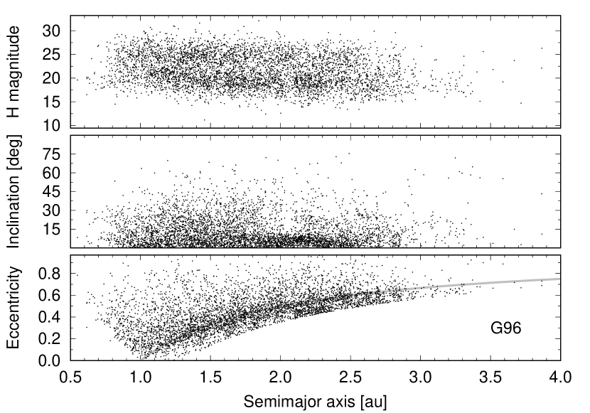
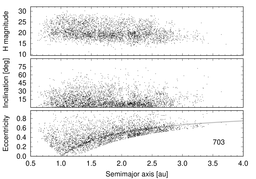
Figure 1: Ecliptic coordinates at discovery for NEOs detected by (top left) G96 and (top right) 703. Observed ($a$,$i$,$e$,$H$) distributions for NEOs detected by (middle left) G96 and (middle right) 703. The gray line in the ($a$,$e$) panels corresponds to $q=1\,\mathrm{au}$. Observed ($q$,$H$) distributions for NEOs detected by (bottom left) G96 and (bottom right) 703.

4 CSS observational selection effects

Figure 2: A 2-d slice through the 4-d detection efficiency, $\epsilon(a,e,i,H)$, with $i=2^{\circ}$ and $H=22.875$ for the G96 survey ($H=22.875$ corresponds to objects of about 100$\,\mathrm{m}$ diameter). To enhance the regions with small efficiency the fig shows $\log\epsilon(a,e,i,H)$ as a function of semi-major axis and eccentricity.

The observed four-dimensional $(a,e,i,H)$ distributions in Fig. 1 are the convolution of the actual distribution of NEOs with the observational selection effects ($\epsilon(a,e,i,H)$) as described in Section 2.1. The calculation of the four-dimensional $\epsilon(a,e,i,H)$ is non-trivial but was performed for the Spacewatch survey (Bottke et al., 2002a), for the Catalina Sky Survey G96 and 703 sites employed herein (Jedicke et al., 2016), and most recently for a combination of many NEO surveys (Tricarico, 2016, 2017). It is impossible to directly compare the calculated detection efficiency in these publications because they refer to different asteroid surveys for different periods of time. The fact that Tricarico (2017)’s final cumulative $H$ distribution is in excellent agreement with the $H$ distribution found in this work suggests that both bias calculations must be accurate to within the available statistics.

The $\epsilon(a,e,i,H)$ slice in Fig. 2 illustrates some of the features of the selection effects that are manifested in the observations shown in Fig. 1. The ‘flat’ region with no values in the lower-right region represents bins that do not contain NEO orbits. The flat region in the lower-left corresponds to orbits that can not be detected by CSS because they are usually too close to the Sun. There is a ‘ridge’ of relatively high detection efficiency along the $q=1\,\mathrm{au}$ line that corresponds to the enhanced detection of objects in the $e$ vs. $a$ panels in Fig. 1. That is, higher detection efficiency along the ridge means that more objects are detected. Perhaps counter-intuitively, the peak efficiency for this $(i,H)$ combination occurs for objects with $(a\sim 1.15\,\mathrm{au},e\sim 0.05)$ while objects on orbits with $1.0\,\mathrm{au}\leq a\leq 1.1\,\mathrm{au}$ are less efficiently detected. This is because the synodic period between Earth and an asteroid with $a=1.1\,\mathrm{au}$ is 11 years but only about 7.5 years for objects with $a=1.15\,\mathrm{au}$, close to the 7-year survey time period considered here. Thus, asteroids with $a=1.1\,\mathrm{au}$ are not detectable as frequently as those with $a=1.15\,\mathrm{au}$. Furthermore, those with smaller semi-major axis have faster apparent rates of motion when they are detectable. Interestingly, the detection efficiency is relatively high for Aten-class objects on orbits with high eccentricity because they are at aphelion and moving relatively slowly when they are detectable in the night sky from Earth.

The bias against detecting NEOs rapidly becomes severe for smaller objects (Supplementary Animation 1 and Supplementary Fig. 1), and only those that have close approaches to the Earth on low-inclination orbits are even remotely detectable. For more details on the bias calculation and a discussion of selection effects in general and for the CSS we refer the reader to Jedicke et al. (2002) and Jedicke et al. (2016).

5 NEO orbit distributions

5.1 Identification of ERs in the MAB

In order to find an exhaustive set of ERs in the MAB Granvik et al. (2017) used the largest MBOs with $H$ magnitudes below the assumed completeness limit and integrated them for 100 Myr or until they entered the NEO region.

Granvik et al. (2017) started from the orbital elements and $H$ magnitudes of the 587,129 known asteroids as listed on July 21, 2012 in the MPC’s MPCORB.DAT file. For MBOs interior to the 3:1 MMR with Jupiter (centered at $a\sim 2.5\,\mathrm{au}$) they selected all non-NEOs ($q>1.3\,\mathrm{au}$) that have $H\leq 15.9$. Exterior to the 3:1 MMR they selected all non-NEOs that have $H\leq 14.4$ and $a<4.1\,\mathrm{au}$. To ensure that the sample is complete they iteratively adjusted these criteria to result in a set of objects that had been discovered prior to Jan 1, 2012—that is, no objects fulfilling the above criteria had been discovered in the $\sim 7$-month period leading to the extraction date.

To guarantee a reasonable accuracy for the orbital elements and $H$ magnitudes Granvik et al. (2017) also required that the selected objects have been observed for at least 30 days, which translates to a relative uncertainty of about 1% for semimajor axis, eccentricity and inclination for MBOs (Muinonen et al., 2006). It is well known that the $H$ magnitudes may have errors of some tenths of a magnitude. However, what is important for the present study is that any systematic effects affect the entire sample in the same way, so that the $H$ cut is done in a similar fashion throughout the MAB. In the end Granvik et al. (2017) were left with a sample of 92,449 MBO orbits where Hungaria and Phocaea test asteroids were cloned 7 and 3 times, respectively (Fig. 3, top and middle). They then assigned a diameter of 100 m and a random spin obliquity of $\pm 90^{\circ}$ to each test asteroid. The test asteroids were integrated with a 1-day timestep for 100 Myr under the influence of a Yarkovsky-driven semimajor-axis drift and accounting for gravitational perturbations by all planets (Mercury through Neptune). During the course of the integrations 70,708 test asteroids entered the NEO region ($q<1.3\,\mathrm{au}$) and their orbital elements were recorded with a time resolution of 10 kyr.

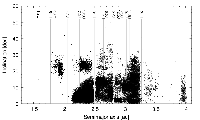
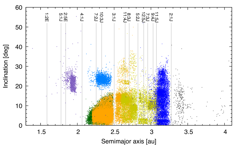
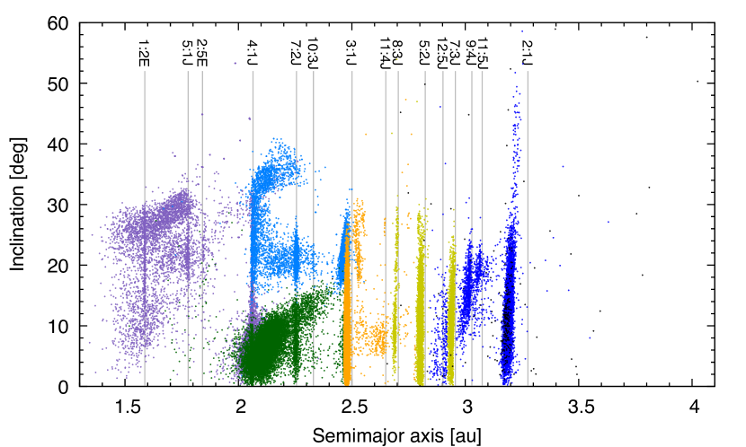
Figure 3: (Top) Initial ($a$,$i$) distribution of test asteroids. (Middle) Initial ($a$,$i$) distribution for test asteroids that entered the NEO region ($q=1.3\,\mathrm{au}$) during the 100-Myr integration. (Bottom) ($a$,$i$) distribution of test asteroids at the time they entered the NEO region ($q=1.3\,\mathrm{au}$). The color coding in the middle and bottom plots correspond to the nominal set of ERs defined in Sec. 6.1. The ERs were defined based on initial orbital elements (Hungarias and Phocaeas) or on orbital elements at the epoch when the test asteroids enter the NEO region (the $\nu_{6}$, 3:1J, 5:2J, and 2:1J complexes).

The orbital elements ($a,e,i,\Omega,\omega,M_{0}$) at the MBO-NEO boundary ($q=1.3\,\mathrm{au}$) define the locations of the escape routes from the MB and form the initial conditions for the NEO residence-time integrations (Fig. 3, bottom). We cloned the test asteroids associated with the $\nu_{6,o}$ SR, and the 7:2J and 8:3J MMRs 5 times to increase the sample in these otherwise undersampled ERs. The total number of test asteroids was thus increased to 80,918.

Our approach to limit ourselves to only 100-m-diameter test asteroids could be problematic because Yarkovsky drift in the MAB may affect the resultant NEO steady-state orbit distribution. The effect would arise because different drift rates imply that asteroids drifting into resonances will spend a different amount of time in or close to the resonances. In cases where the bodies are drifting slowly, they could become trapped in tiny resonances and pushed out of the MAB prior to when our model results predict (e.g., Nesvorný and Morbidelli, 1998; Bottke et al., 2002b). In other cases, SRs such as the $\nu_{6}$ with the adjacent $\nu_{16}$ can change the inclination of the asteroid (Froeschle and Scholl, 1986; Scholl and Froeschle, 1986) and the amount of change depends on the time it takes for the asteroid to evolve to the NEO region. Unfortunately, we are not yet at the point where full-up models including accurate representations of the Yarkovsky and YORP effects can be included for tens of thousands of asteroids across the MAB. Our work in this paper represents a compromise between getting the dynamics as correct as possible and ensuring computational expediency. Our main concern here is that using a drift rate that varies with size could lead to steady-state orbit distributions that are correlated with asteroid diameter.

To test this scenario we selected the test asteroids in set ’B’ in Granvik et al. (2017) that entered the NEO region and produced steady-state distributions for $D=0.1\,\mathrm{km}$ and $D=3\,\mathrm{km}$ NEOs that escape through the 3:1J MMR and the $\nu_{6}$ SR. There was thus a factor of 30 difference in semimajor-axis drift rate. To save time we decided to continue the integrations for only up to 10 Myr instead of integrating all test asteroids until they reach their respective sinks. Since the average lifetime of all NEOs is $\lesssim 10$ Myr this choice nevertheless allowed most test asteroids to reach their sinks. We then discretized and normalized the distributions (Eq. 4), and computed the difference between the distributions for small and large test asteroids.

In the case of the 3:1J MMR we found no statistically significant differences in NEO steady-state orbit distributions between large and small test asteroids when compared to the noise (Supplementary Fig. 2). For $\nu_{6}$ we found that while the “signal” is stronger compared to 3:1J so is the noise for the $D=3\,\mathrm{km}$ case. A priori we would expect a stronger effect for the $\nu_{6}$ resonance because the semi-major axis drift induced by the Yarkovsky effect can change the position of the asteroid relative to an SR, but not relative to an MMR, which reacts adiabatically. However, based on our numerical simulations we concluded that the Yarkovsky drift in the MAB results in changes in the NEO steady-state orbit distributions that are negligible for the purposes of our work. Therefore we decided to base the orbital integrations, that are required for constructing the steady-state NEO orbit distributions, on the test asteroids with $D=0.1\,\mathrm{km}$ that escape the MAB (Granvik et al., 2017).

5.2 Orbital evolution of NEOs originating in the MAB

Next we continued the forward integration of the orbits of the 80,918 100-meter-diameter test asteroids that entered the NEO region with a slightly different configuration as compared to the MBO integrations described in the previous subsection. To build smooth orbit distributions we recorded the elements of all test asteroids with a time resolution of 250 yr. The average change in the orbital elements over 250 yr based on our integrations is $\Delta a=0.004\,\mathrm{au}$, $\Delta e=0.006$, and $\Delta i=0.728^{\circ}$. The average change sets a limit on the resolution of the discretized orbit distribution in order to avoid artefacts, although the statistical nature of the steady-state orbit distribution softens discontinuities in the orbital tracks of individual test asteroids.

A non-zero Yarkovsky drift in semimajor axis has been measured for tens of known NEOs (Chesley et al., 2003; Nugent et al., 2012; Farnocchia et al., 2013; Vokrouhlický et al., 2015), but the common assumption is that over the long term the Yarkovsky effect on NEO orbits is dwarfed by the strong orbital perturbations caused by their frequent and close encounters with terrestrial planets. For a km-scale asteroid the typical measured drift in semimajor axis caused by the Yarkovsky effect is $\sim 2\times 10^{-4}\,\mathrm{au}\,\mathrm{Myr}^{-1}$ or $\sim 5\times 10^{-8}\,\mathrm{au}\,(250\,\mathrm{yr})^{-1}$ whereas the average change of semimajor axis for NEOs from (size-independent) gravitational perturbations is $\sim 4\times 10^{-3}\,\mathrm{au}\,(250\,\mathrm{yr})^{-1}$. The rate of change of the semimajor axis caused by Yarkovsky is thus several orders of magnitude smaller than that caused by gravitational perturbations. We concluded that the effect of the Yarkovsky drift on the NEO steady-state orbit distribution is negligible compared to the gravitational perturbations caused by planetary encounters. Hence we omitted Yarkovsky modeling when integrating test asteroids in the NEO region.

Integrations using a 1-day timestep did not correctly resolve close solar encounters. This results in the steady-state orbital distribution at low $a$ and large $e$ to be very ”unstable”, as one can see by comparing the distributions in the top left corners of the ($a,e$) plots in Supplementary Fig. 1, obtained by selecting alternatively particles with even or odd identification numbers. So we reduced the nominal integration timestep to 12 hours and restarted the integrations. These NEO integrations required on the order of 2 million CPU hours and solved the problem (see top left corners of left-hand-side ($a,e$) plots in Figs. 4 and 5). We note that Greenstreet et al. (2012a) used a timestep of only 4 hours to ensure that encounters with Venus and Earth are correctly resolved even in the fastest encounters. Considering that the required computing time would have tripled if we had used a four-hour integration step and considering that all the evidence we have suggests that the effect is negligible, we saw no obvious reason to reduce the timestep by an additional factor of 3. We stress, however, that the integration step is automatically substantially reduced when the integrator detects a planetary encounter.

The orbital integrations continued until every test asteroid had collided with the Sun or a planet (Mercury through Neptune), escaped the solar system or reached a heliocentric distance in excess of $100\,\mathrm{au}$. For the last possibility we assume that the likelihood of the test asteroid re-entering the NEO region ($a<4.2\,\mathrm{au}$) is negligible as it would have to cross the outer planet region without being ejected from the solar system or colliding with a planet. The longest lifetimes among the integrated test asteroids are several Gyr.

Out of the 80,918 test asteroids about to enter the NEO region we followed 79,804 (98.6%) to their respective sink. The remaining 1.4% of the test asteroids did not reach a sink for reasons such as ending up in a stable orbit with $q>1.3\,\mathrm{au}$. As the Yarkovsky drift was turned off these orbits were found to remain virtually stable over many Gyr and thus the test asteroids were unable to drift into resonances that would have brought them back into the NEO region. In addition, the output data files of some test asteroids were corrupted, and in order not to skew the results we omitted the problematic test asteroids when constructing the NEO steady-state orbit distributions.

5.2.1 NEO lifetimes and sinks

As expected, the most important sinks are i) a collision with the Sun and ii) an escape from the inner solar system after a close encounter with, primarily, Jupiter (Table 3).

Table 3: Fraction of test asteroids ending up in various sinks (collisions with the Sun or planets, or an escape from the inner solar system, $a>100\,\mathrm{au}$) and mean lifetime of test asteroids in the NEO region ($q<1.3\,\mathrm{au}$, $a<4.2\,\mathrm{au}$, $e<1$, $i<180^{\circ}$) as a function of the ER that is provided in the left column. We provide four different scenarios for each ER-sink pair: no thermally-driven destruction at small $q$, and thermally-driven destruction when $q<0.058\,\mathrm{au}$, $q<0.076\,\mathrm{au}$, $q<0.184\,\mathrm{au}$. The three perihelion distances correspond to km-scale, average, and dm-scale NEOs (Granvik et al., 2016). The horizontal lines divides the ERs into the six asteroidal groups that are used for the nominal model in Sec. 6.2. Note that the relatively high fraction of Earth-impacts from 11:5J is due to small number statistics.

ER	# of test	Sun	Mercury	Venus	Earth	Mars	Jupiter	Escape	$\langle L\rangle$
	asteroids	[%]	[%]	[%]	[%]	[%]	[%]	[%]	[Myr]
Hungaria
Hung.	8128	77.5/0.0/0.0/0.0	1.1/0.7/0.6/0.3	6.2/4.9/4.6/3.4	6.4/5.4/5.2/4.3	2.2/2.1/2.0/2.0	0.1/0.1/0.1/0.1	6.9/5.8/5.6/4.1	43.3/37.2/36.0/32.5
$\nu_{6}$ complex
$\nu_{6}$	13029	81.2/0.0/0.0/0.0	0.5/0.4/0.3/0.1	2.5/2.0/1.9/1.4	2.3/1.9/1.8/1.5	0.4/0.4/0.4/0.4	0.2/0.2/0.2/0.1	12.9/11.8/11.3/8.4	9.4/7.2/6.8/5.5
4:1	1899	75.8/0.0/0.0/0.0	0.7/0.5/0.5/0.2	4.4/3.7/3.6/2.5	3.7/3.2/3.1/2.8	0.2/0.2/0.2/0.2	0.1/0.1/0.1/0.1	15.2/14.0/13.5/9.7	10.2/8.5/8.2/6.6
7:2	4969	83.2/0.0/0.0/0.0	0.1/0.1/0.1/0.1	1.2/0.9/0.8/0.5	1.3/1.1/1.1/0.9	0.3/0.3/0.3/0.2	0.3/0.3/0.3/0.2	13.7/12.5/12.1/8.9	6.7/5.5/5.3/4.2
Phocaea
Phoc.	8309	89.5/0.0/0.0/0.0	0.2/0.1/0.1/0.0	1.3/1.0/0.9/0.5	1.0/0.6/0.6/0.4	0.4/0.3/0.3/0.3	0.1/0.0/0.0/0.0	7.9/5.0/4.7/2.9	14.3/11.2/10.7/8.9
3:1J complex
3:1J	7753	76.1/0.0/0.0/0.0	0.1/0.0/0.0/0.0	0.4/0.4/0.3/0.2	0.2/0.1/0.1/0.1	0.0/0.0/0.0/0.0	0.6/0.5/0.5/0.4	22.6/20.4/19.7/14.6	2.2/1.5/1.3/0.9
$\nu_{6,o}$	3792	70.9/0.0/0.0/0.0	0.0/0.0/0.0/0.0	0.2/0.1/0.1/0.1	0.3/0.2/0.2/0.2	0.2/0.2/0.2/0.2	0.3/0.3/0.3/0.3	28.1/26.1/25.3/22.4	3.5/2.5/2.3/1.9
5:2J complex
8:3J	3080	45.1/0.0/0.0/0.0	0.0/0.0/0.0/0.0	0.0/0.0/0.0/0.0	0.2/0.2/0.2/0.2	0.0/0.0/0.0/0.0	1.0/1.0/1.0/1.0	53.6/50.6/49.9/46.1	2.2/1.7/1.6/1.4
5:2J	5955	16.9/0.1/0.1/0.1	0.0/0.0/0.0/0.0	0.1/0.1/0.1/0.1	0.1/0.1/0.1/0.1	0.0/0.0/0.0/0.0	1.2/1.1/1.1/1.1	81.8/79.4/78.8/75.0	0.5/0.4/0.4/0.3
7:3J	2948	7.4/0.0/0.0/0.0	0.0/0.0/0.0/0.0	0.0/0.0/0.0/0.0	0.0/0.0/0.0/0.0	0.0/0.0/0.0/0.0	1.1/1.1/1.1/1.1	91.5/90.2/89.7/87.7	0.2/0.2/0.2/0.2
2:1J complex
9:4J	443	25.3/0.0/0.0/0.0	0.0/0.0/0.0/0.0	0.0/0.0/0.0/0.0	0.0/0.0/0.0/0.0	0.0/0.0/0.0/0.0	0.9/0.9/0.9/0.9	73.8/69.3/68.2/63.0	0.5/0.4/0.4/0.3
$z_{2}$	929	14.3/0.1/0.1/0.1	0.0/0.0/0.0/0.0	0.0/0.0/0.0/0.0	0.0/0.0/0.0/0.0	0.0/0.0/0.0/0.0	1.3/1.2/1.2/1.0	84.4/82.1/81.5/77.7	0.6/0.3/0.3/0.3
11:5J	133	43.6/0.0/0.0/0.0	0.0/0.0/0.0/0.0	0.0/0.0/0.0/0.0	0.8/0.8/0.8/0.8	0.0/0.0/0.0/0.0	0.8/0.8/0.0/0.0	54.9/47.4/45.9/39.8	0.5/0.4/0.4/0.4
2:1J	5321	22.1/0.3/0.2/0.1	0.0/0.0/0.0/0.0	0.0/0.0/0.0/0.0	0.1/0.1/0.1/0.1	0.0/0.0/0.0/0.0	1.0/0.9/0.9/0.8	76.8/70.8/69.2/61.5	0.5/0.4/0.4/0.3

The estimation of NEO lifetimes, that is, the time asteroids and comets spend in the NEO region before reaching a sink when starting from the instant when they enter the NEO region (that is, $q\leq 1.3\,\mathrm{au}$ for the first time), is complicated by the fact that NEOs are also destroyed by thermal effects (Granvik et al., 2016). The typical heliocentric distance for a thermal disruption depends on the size of the asteroid. For large asteroids with $D\gtrsim 1\,\mathrm{km}$ the typical perihelion distance at which the disruption happens is $q\sim 0.058\,\mathrm{au}$. We see a 10–50% difference in NEO lifetimes when comparing the results computed with and without thermal disruption (Table 3). For smaller asteroids the difference is even greater because the disruption distance is larger.

We define the mean lifetime of NEOs to be the average time it takes for test asteroids from a given ER to reach a sink when starting from the time that they enter the NEO region. Our estimate for the mean lifetime of NEOs originating in the 3:1J MMR is comparable to that provided by Bottke et al. (2002a), but for $\nu_{6}$ and the resonances in the outer MAB our mean lifetimes are about 50% and 200% longer, respectively (Table 3). These differences can, potentially, be explained by different initial conditions and the longer timestep used for the integrations carried out by Bottke et al. (2002a). A longer timestep would have made the orbits more unstable than they really are and close encounters with terrestrial planets would not have been resolved. An accurate treatment of close encounters would pull out test asteroids from resonances whereas an inability to do this would lead to test asteroids rapidly ending up in the Sun and thereby also to a shorter average lifetime.

5.2.2 Steady-state orbit distributions and their uncertainties

We combined the evolutionary tracks of test asteroids that enter the NEO region through 12 ERs and from 2 additional SRs into 6 steady-state orbit distributions by summing up the time that the test asteroids spend in various parts of the binned ($a,e,i$) space (left column in Figs. 4 and 5).

To understand the statistical uncertainty of the orbit distributions, we divided the test asteroids for each orbit distribution into even-numbered and odd-numbered groups and estimated the uncertainty of the overall orbit distribution by computing the difference between the orbit distributions composed of even-numbered and odd-numbered test asteroids. The difference distribution was then normalized by using the combined orbit distribution so as to result in a distribution with the same units as the combined distribution (right column in Figs. 4 and 5).

Hungarias

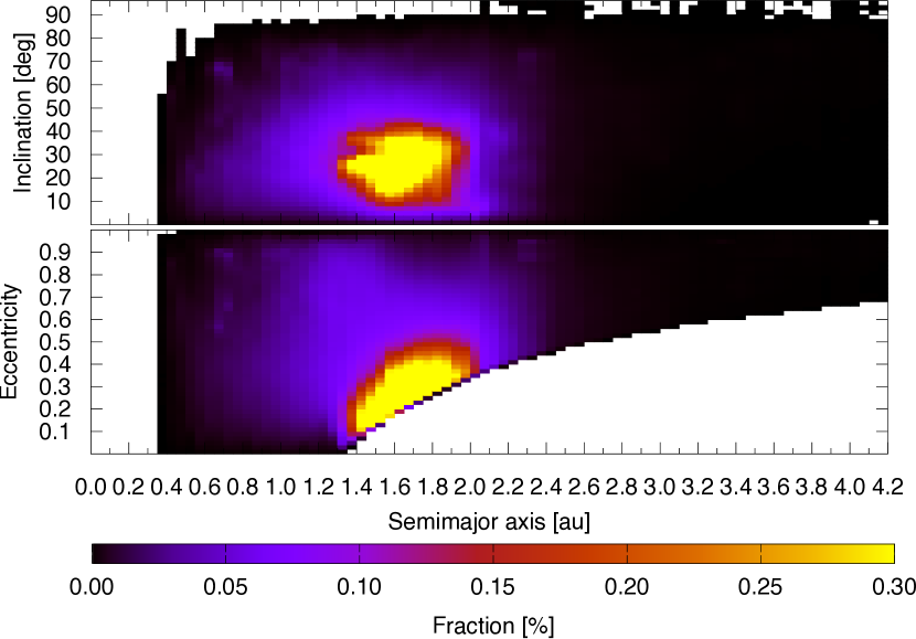
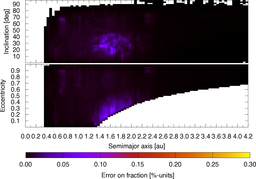
$\nu_{6}$ complex

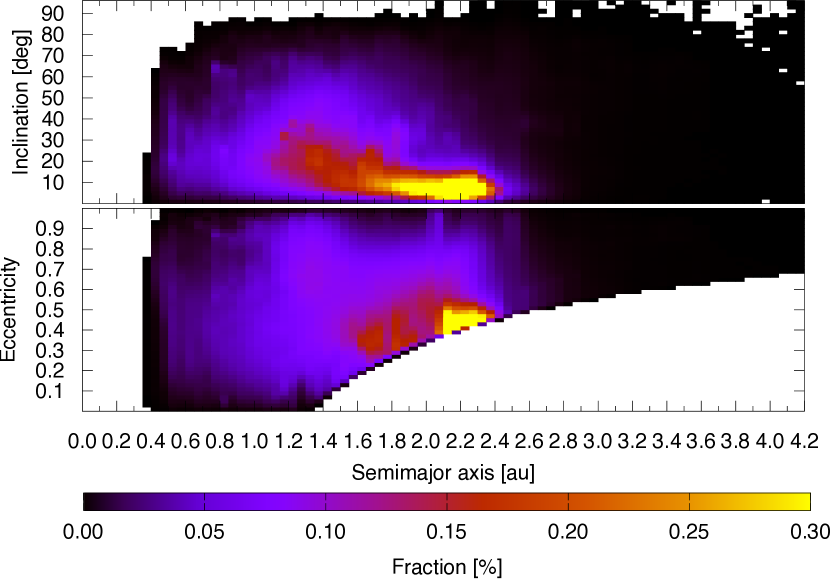
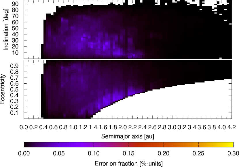
Phocaeas

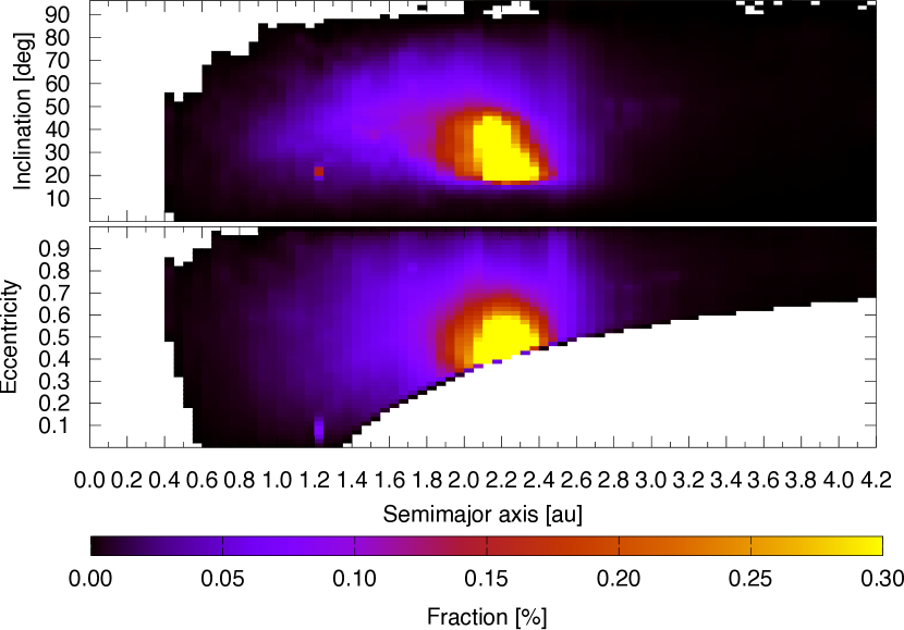
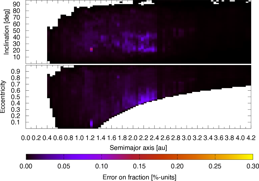
Figure 4: Steady-state orbit distributions (left) and the corresponding uncertainty distributions (right) for NEOs originating in asteroidal ERs: Hungarias (top panel), $\nu_{6}$ complex (middle panel), and Phocaeas (bottom panel).

3:1J complex
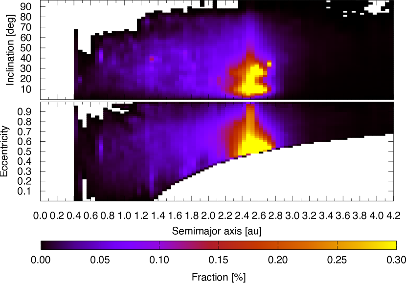
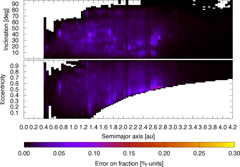
5:2J complex
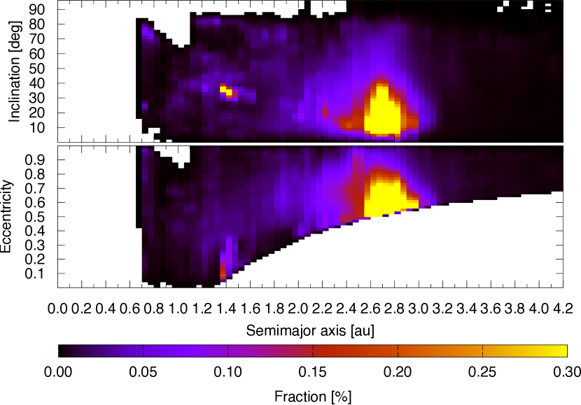
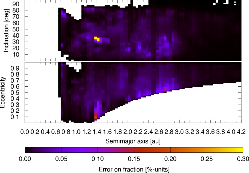
2:1J complex

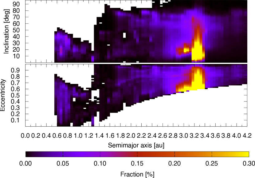
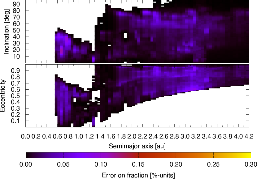
Figure 5: Steady-state orbit distributions (left) and the corresponding uncertainty distributions (right) for NEOs originating in asteroidal ERs: 3:1J (top panel), 5:2J complex (middle panel), and 2:1J complex (bottom panel).

5.2.3 JFC steady-state orbit distribution

There are several works in the published literature which computed the steady-state orbital distribution of Jupiter-family comets by integrating particles coming from the trans-Neptunian region up to their ultimate dynamical removal. The pioneering work was that of Levison and Duncan (1997), followed by Levison et al. (2006), Di Sisto et al. (2009), and Brasser and Morbidelli (2013). The resulting JFC orbital distributions have been kindly provided to us by the respective authors. We have compared them and selected the one from the Levison et al. (2006) work because it is the only one constructed using simulations that accounted for the gravitational perturbations by the terrestrial planets. Thus, unlike the other distributions, this one includes ”comets” on orbits decoupled from the orbit of Jupiter (i.e., not undergoing close encounters with the giant planet at their aphelion) such as comet Encke. We think that this feature is important to model NEOs of trans-Neptunian origin. We remind the reader that Bottke et al. (2002a) used the JFC distribution from Levison and Duncan (1997), given that the results of Levison et al. (2006) were not yet available. Thus, this is another improvement of this work over Bottke et al. (2002a). The JFC orbital distribution we adopted is shown in Fig. 6.

There is an important difference between what we have done in this work and what was done in the earlier models of the orbital distribution of active JFCs because they included a JFC fading parameter. In essence, a comet is considered to become active when its perihelion distance decreases below some threshold (typically 2.5 au) for the first time. That event starts the ”activity clock”. Particles are assumed to contribute to the distribution of JFCs only up to a time $T_{\rm active}$ of the activity clock. Limiting the physical lifetime is essential to reproduce the observed inclination distribution of active JFCs, as first shown in Levison and Duncan (1997). What happens after $T_{\rm active}$ is not clear. The JFCs might disintegrate or they may become dormant. Only in the second case, of course, can the comet contribute to the NEO population with an asteroidal appearance. We believe the second case is much more likely because JFCs are rarely observed to disrupt, unlike long period comets. Besides, several studies argued for the existence of dormant JFCs (e.g., Fernández et al., 2005; Fernández and Morbidelli, 2006). Thus, in order to build the distribution shown in Fig. 6 we have used the original numerical simulations of Levison et al. (2006) but suppressed any limitation on a particle’s age.

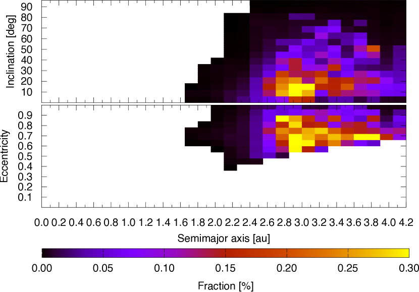
Figure 6: JFC steady-state orbit distribution.

6 Debiased NEO orbit and absolute-magnitude distributions

6.1 Selecting the preferred combination of steady-state orbit distributions

We first needed to find the optimum combination of ERs. To strike a quantitative balance between the goodness of fit and the number of parameters we used the AICc metric defined by Eq. (12). We tested 9 different ER models out of which all but one are based on different combinations of the steady-state orbit distributions described in Sect. 5. The one additional model is the integration of Bottke-like initial conditions by Greenstreet et al. (2012a). The combination of different ERs was done by summing up the residence-time distributions of the different ERs, that is, prior to normalizing the orbit distributions. Hence the initial orbit distribution and the direct integrations provided the relative shares between the different orbit distributions that were combined.

As expected, the maximum likelihood (ML) constantly improves as the steady-state orbit distribution is divided into a larger number of subcomponents (Fig. 7). The ML explicitly shows that our steady-state orbit distributions lead to better fits compared to the Bottke-like orbit distributions by Greenstreet et al. (2012a), even when using the same number of ERs, that is, four asteroidal and one cometary ER. The somewhat unexpected outcome of the analysis is that we do not find a minimum for the AICc metric, which would have signaled an optimum number of model parameters (Fig. 7). Instead the AICc metric improves all the way to the most complex model tested which contains 23 different ERs and hence 94 free parameters!

Figure 7: The log-likelihood of the best-fit solution (left axis and solid line) and the corresponding AICc metric (right axis and dashed line) as a function of the number of ERs included in the model. G12 stands for the five-component orbit model by Greenstreet et al. (2012a).

The largest drop in AICc per additional source takes place when we go from a five-component model to a six-component model. The difference between the two being that the former divides the outer MAB into two components and lack Hungarias and Phocaeas whereas the latter has a single-component outer-MAB ER and includes Hungarias and Phocaeas. Continuining to the seven-component model we again split up the outer-MAB ER into two components (the 5:2J and 2:1J complexes). The difference between the five-component model and the seven-component model is thus the inclusion of Hungarias and Phocaeas in the latter. The dramatic improvement in AICc shows that the Hungarias and Phocaeas are relevant components of an NEO orbit model.

Although a model with 94 free parameters is formally acceptable, we had some concern that it would lead to degenerate sets of model parameters. It might also (partly) hide real phenomena that are currently not accounted for and thus should show up as a disagreement between observations and our model’s predictions. Therefore we took a heuristic approach and compared the steady-state orbit distributions to identify those that are more or less overlapping and can thus be combined. After a qualitative evaluation of the orbit distributions we concluded that it is sensible to combine the asteroidal ERs into six groups (Figs. 4 and 5). Of these six groups the Hungaria and Phocaea orbit distributions are uniqely defined based on the initial orbits of the test asteroids whereas the four remaining groups are composed of complexes of escape routes ($\nu_{6}$, 3:1J, 5:2J, and 2:1J) that produce overlapping steady-state orbit distributions.

In principle one could argue, based on Fig. 7, that it would make sense to use 9 ERs because then the largest drop in the AICc metric would have been accounted for. The difference between 7 and 9 ERs is that the 4:1J has been separated from the $\nu_{6}$ complex (Fig. 8) and the $\nu_{6}$ component external to the 3:1J has been separated from the 3:1J (Fig. 9). However, the differences between the $\nu_{6}$ complex and the 4:1J orbit distributions are small with the most notable difference being that the $\nu_{6}$ distribution extends to larger $a$. Similarly, the $\nu_{6}$ component external to the 3:1J has some clear structure compared to the 3:1J component but this structure is also clearly visible in the combined 3:1J orbit distribution (top panel in Fig. 5). There is thus a substantial overlap in the orbit distributions and we therefore decided to include one cometary and six asteroidal ERs in the model.

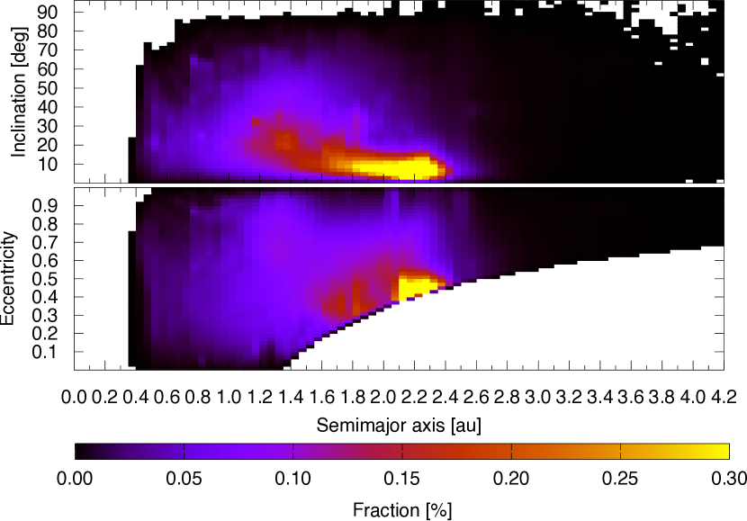
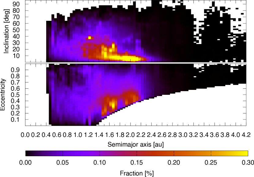
Figure 8: Steady-state orbit distributions for $\nu_{6}$ and 7:2J (top) and 4:1J (bottom).

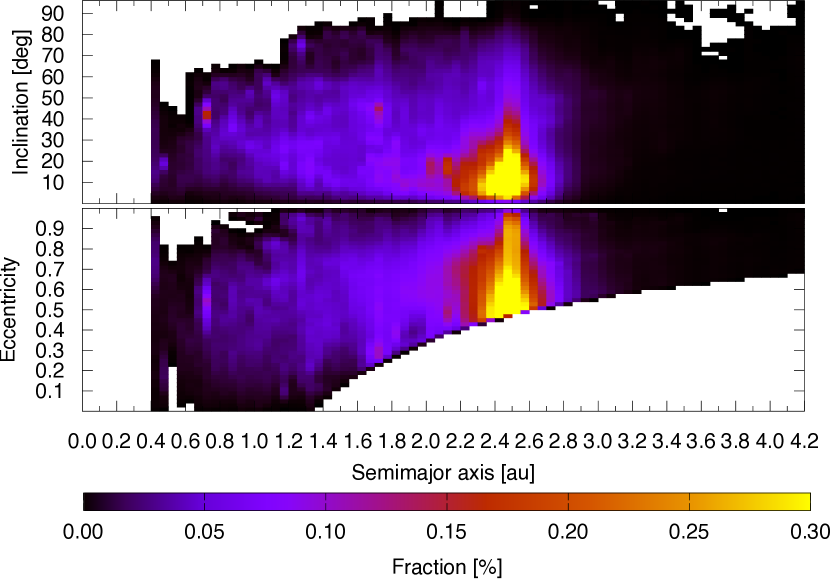
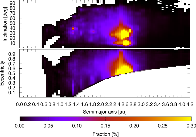
Figure 9: Steady-state orbit distributions for 3:1J (top) and the low-$i$ and high-$i$ components of the outer $\nu_{6}$ (bottom).

6.2 The best-fit model with 7 ERs

Having settled on using 7 steady-state orbit distributions for the nominal model we then turned to analyzing the selected model in greater detail. As described in the Introduction, it is impossible to reach an acceptable agreement between the observed and predicted orbit distribution unless the disruption of NEOs at small $q$ is accounted for (Granvik et al., 2016). Here we solved the discrepancy by fitting for the two parameters that describe a penalty function against NEOs with small $q$ (see Sect. 2), in addition to the parameters describing the $H$ distributions. The best-fit parameters for the penalty function are $k=1.40\pm 0.07\,\mathrm{au}^{-1}$ and $q_{0}=0.69\pm 0.02\,\mathrm{au}$. Although a direct comparison of the best-fit penalty function and the physical model by Granvik et al. (2016) is impossible we find that the penalty function $p=0.86\pm 0.05$ at $q=0.076\,\mathrm{au}$ and, of course, even higher for $q<0.076\,\mathrm{au}$. Considering that the 3$\sigma$ value at $q=0.076\,\mathrm{au}$ reaches unity we find the agreement satisfactory.

A comparison between the observed and predicted number (i.e., marginal distributions of $\epsilon(a,e,i,H)\,N(a,e,i,H)$) of NEO detections shows that the best-fit model accurately reproduces the observed ($a$,$e$,$i$,$H$) distributions (Fig. 10) as well as the observed $q$ distribution (Fig. 11). Thus the penalty function is able to mitigate the problem caused by not including a physical model of NEO disruptions close to the Sun.

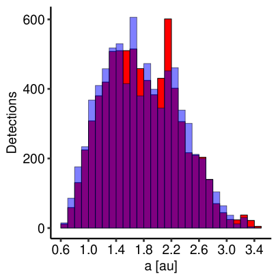
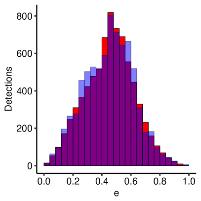
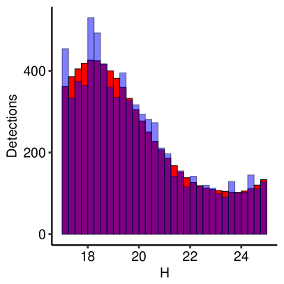
Figure 10: Comparison between G96 and 703 detections (blue; $n(a,e,i,H)$) and prediction based on the best-fit model (red; $\epsilon(a,e,i,H)\,N(a,e,i,H)$). The purple color indicates overlapping distributions.

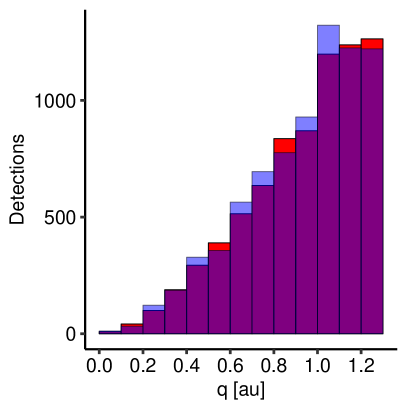
Figure 11: As Fig. 10 but for perihelion distance $q$.

We used the same approach as Bottke et al. (2002a) to evaluate the statistical uncertainty of the 28 parameters (four parameters for each of the 7 HFDs and two parameters for the penalty function) that define our model. We first generated 100 random realizations of the biased best-fit four-dimensional model (the marginal distributions of which are shown in red in Fig. 10). Each realization contains 7,769 virtual detections, that is, the number of detections reported by the G96 and 703 surveys that we used for the nominal fit. When re-fitting the model to each of these synthetic data sets we obtained slightly different values for the best-fit parameters (Supplementary Figs. 3 and 4), which we interpret as being caused by the statistical uncertainty. Note that the parameter distributions are often non-Gaussian but nevertheless relatively well constrained.

We interpret the RMS with respect to the best-fit parameters obtained for the real data to be a measure of the statistical uncertainty for the parameters. The best-fit parameters describing the HFDs as well as their uncertainties are reported in Table 4. The best-fit parameters for the penalty function are $k=1.40\pm 0.07$ and $q_{0}=0.69\pm 0.02$. The minimum HFD slope is statistically distinct from zero only for $\nu_{6}$ and 3:1J and the slope minimum typically occurs around $H\sim 20$. This implies that the HFD slope should be at its flattest around $H\sim 20$ as seen in the apparent $H$ distribution observed by G96 (Fig. 1). A constant slope is acceptable (curvature within 1$\sigma$ of zero) only for Phocaeas and 5:2J, which shows that the decision to allow for a more complex functional form for the HFDs law was correct.

Table 4: The best-fit model parameters $N_{0}(H_{0}=17)$, $c$, $H_{\rm min}$, and $\alpha_{\rm min}$. The average lifetime $\langle L\rangle$ in NEO region ($q<1.3\,\mathrm{au}$ and $a<4.2\,\mathrm{au}$) as computed from the orbital integrations. The model prediction for the debiased number of NEOs $N(17<H<22)$ and $N(17<H<25)$; the relative fraction of NEOs from each ER $\beta(17<H<22)$ and $\beta(17<H<25)$; the absolute flux of NEOs from each ER into the NEO region $F(17<H<22)$ and $F(17<H<25)$; and the relative flux of NEOs from each ER into the NEO region $\gamma(17<H<22)$ and $\gamma(17<H<25)$.

ER	Hungaria	$\nu_{6}$ complex	Phocaea	3:1J complex	5:2J complex	2:1J complex	JFC
$N_{0}(H_{0}=17)$	$23.1\pm 3.0$	$34.6\pm 2.6$	$10.3\pm 3.7$	$25.1\pm 6.0$	$19.3\pm 5.1$	$3.6\pm 1.9$	$6.6\pm 2.6$
$c$	$0.013\pm 0.007$	$0.037\pm 0.003$	$0.008\pm 0.027$	$0.009\pm 0.007$	$0.008\pm 0.019$	$0.062\pm 0.023$	$0.024\pm 0.019$
$H_{\rm min}$	$15.6\pm 1.5$	$20.4\pm 0.1$	$23.4\pm 3.9$	$18.0\pm 4.6$	$25.0\pm 3.0$	$20.9\pm 0.8$	$18.0\pm 2.1$
$\alpha_{\rm min}$	$0.00\pm 0.06$	$0.24\pm 0.01$	$0.00\pm 0.09$	$0.33\pm 0.10$	$0.00\pm 0.10$	$0.00\pm 0.04$	$0.12\pm 0.08$
$\langle L\rangle$ [Myr]	$37.19\pm 0.23$	$6.98\pm 0.50$	$11.16\pm 0.37$	$1.83\pm 0.03$	$0.68\pm 0.11$	$0.40\pm 0.05$	–
$N(17<H<22)$	$1,400^{+130}_{-160}$	$11,470^{+280}_{-220}$	$670^{+190}_{-110}$	$7,250^{+420}_{-480}$	$3,020^{+290}_{-290}$	$890^{+120}_{-70}$	$470^{+100}_{-80}$
$\beta(17<H<22)$	$0.056^{+0.005}_{-0.007}$	$0.456^{+0.011}_{-0.009}$	$0.027^{+0.008}_{-0.004}$	$0.288^{+0.017}_{-0.019}$	$0.120^{+0.012}_{-0.012}$	$0.035^{+0.005}_{-0.003}$	$0.019^{+0.004}_{-0.003}$
$F(17<H<22)$ [Myr-1]	$38^{+4}_{-4}$	$1,640^{+130}_{-120}$	$60^{+17}_{-10}$	$3,950^{+240}_{-270}$	$4,420^{+860}_{-860}$	$2,200^{+410}_{-330}$	–
$\gamma(17<H<22)$	$0.003^{+0.001}_{-0.001}$	$0.133^{+0.010}_{-0.010}$	$0.005^{+0.001}_{-0.001}$	$0.321^{+0.019}_{-0.022}$	$0.359^{+0.070}_{-0.070}$	$0.179^{+0.033}_{-0.027}$	–
$N(17<H<25)$	$143,500^{+26,200}_{-26,600}$	$296,400^{+17,800}_{-16,500}$	$1,300^{+25,200}_{-200}$	$286,400^{+25,200}_{-34,000}$	$7,200^{+15,400}_{-800}$	$4,400^{+7,900}_{-1,200}$	$62,700^{+11,600}_{-12,200}$
$\beta(17<H<25)$	$0.179^{+0.033}_{-0.033}$	$0.370^{+0.022}_{-0.021}$	$0.002^{+0.031}_{-0.000}$	$0.357^{+0.031}_{-0.042}$	$0.009^{+0.019}_{-0.001}$	$0.005^{+0.010}_{-0.001}$	$0.078^{+0.014}_{-0.015}$
$F(17<H<25)$ [Myr-1]	$3,900^{+700}_{-700}$	$42,500^{+4000}_{-3900}$	$100^{+2300}_{-20}$	$156,100^{+14,000}_{-18,700}$	$10,600^{+22,600}_{-2,100}$	$10,900^{+19,600}_{-3,200}$	–
$\gamma(17<H<25)$	$0.017^{+0.003}_{-0.003}$	$0.190^{+0.018}_{-0.017}$	$0.0005^{+0.0103}_{-0.0001}$	$0.697^{+0.062}_{-0.083}$	$0.047^{+0.101}_{-0.009}$	$0.049^{+0.087}_{-0.014}$	–

Figure 12 shows a graphical representation of the parameters describing the HFDs (Table 4). The statistical uncertainty for the number of Phocaeas, 5:2J, 2:1J and JFCs is around 1–2 orders of magnitude for $H\gtrsim 23$ whereas the uncertainty for Hungarias, $\nu_{6}$ and 3:1J is within a factor of a few throughout the $H$ range. The explanation for the large uncertainties for the former group is that their absolute observed numbers are smaller than for the NEOs originating in the latter group and hence their numbers are more difficult to constrain.

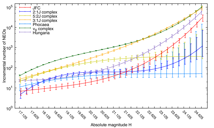
Figure 12: Debiased, incremental absolute-magnitude distributions for NEOs from different ERs.

The ratio between the HFD for each ER and the overall HFD shows that the contribution from the different ERs varies as a function of $H$ (Fig. 13). The $\nu_{6}$ and 3:1J complexes are the largest contributors to the steady-state NEO population regardless of $H$ as expected. The $\nu_{6}$ dominates the large NEOs whereas the 3:1J is equally important at about $D\sim 100\,\mathrm{m}$. The Hungarias and JFCs have a non-negligible contribution throughout the $H$ range whereas Phocaeas and the 5:2J and 2:1J complexes have a negligible contribution at small sizes.

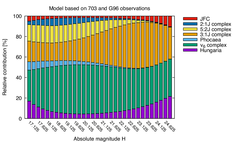
Figure 13: Relative importance of 7 different NEO ERs as a function of the absolute magnitude.

The varying contribution from different ERs as a function of $H$ leads to the overall orbit distribution also varying with $H$ despite the fact that the ER-specific orbit distributions do not vary (Supplementary Animation 2 and Supplementary Fig. 5).

Next we propagated the uncertainties of the model parameters into the number of objects in each cell of the ($a$,$e$,$i$,$H$) space. Even though the errors in individual cells can be larger than 100% (particularly when the expected population in the cell is small) the overall statistical uncertainty on the number of NEOs with $H<25$ is $\lesssim 5$% (Table 5).

Table 5: Absolute and relative shares belonging to 5 NEO classes based on the number-weighted average over $17<H<25$. The uncertainty estimates only account for the random component.

NEO class	$N(17<H<25)$	Relative share [%]
Amor	$316,000^{+19,000}_{-12,000}$	$39.4^{+2.3}_{-1.5}$
Apollo	$436,000^{+21,000}_{-12,000}$	$54.4^{+2.6}_{-1.5}$
Aten	$27,700^{+900}_{-800}$	$3.46^{+0.12}_{-0.10}$
Atira	$9,200^{+300}_{-300}$	$1.15^{+0.04}_{-0.03}$
Vatira	$1,970^{+60}_{-70}$	$0.25^{+0.01}_{-0.01}$

Given that the relative importance of the 7 ERs vary substantially with $H$ (Fig. 13) it is somewhat surprising that the relative shares of the 4 different NEO classes is hardly changing with $H$ (Fig. 14).

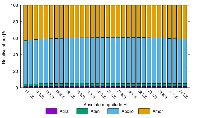
Figure 14: Relative shares between the 4 main NEO classes as a function of the absolute magnitude.

Another consequence of the varying contribution from different ERs as a function of $H$ is that also the average lifetime of NEOs changes with $H$ when weighted by the relative contribution from each ER (Fig. 15). The average lifetime ranges from about 6 to 11 Myr with the mid-sized NEOs having the shortest lifetimes. The increased average lifetime for both the largest and the smallest NEOs considered is driven by the contribution from the Hungaria ER, because NEOs from that ER have about 4–100 times longer lifetimes than NEOs from the other ERs considered. Note also the clear correlation between the average lifetime and the relative contribution of the Hungaria ER (Fig. 13).

Figure 15: The average lifetime of NEOs as a function of absolute magnitude $H$ weighted by the relative contribution from each ER.

The analysis above does not account for the systematic uncertainties arising, for instance, from an imperfect evaluation of the biases or of the construction of the steady-state orbit distributions of the NEOs coming from the various ERs. We will next assess systematic uncertainties quantitatively by i) comparing models constructed using two independent sets of orbit distributions (Sect. 6.3), and ii) by comparing models based on two independent surveys (Sect. 6.4).

6.3 Sensitivity to variations in orbit distributions

To assess the sensitivity of the model on statistical variations in the 7 included steady-state orbit distributions corresponding to the ERs we divided the test asteroids into even-numbered and odd-numbered sets to construct two independent orbit distributions. Then we constructed the biased marginal $a$, $e$, $i$, and $H$ distributions by using the two sets of orbit distributions and the best-fit parameters found for the nominal model (Table 4). A comparison of the biased distributions with the observed distributions show that both sets of orbit distributions lead to an excellent agreement between model and observations (Fig. 16). The largest discrepancy between the biased marginal distributions is found for the $a$ and $e$ distributions ($a\sim 1.3\,\mathrm{au}$ and $e\sim 0.2$). In general, the variations in the orbit distributions are small and the systematic uncertainties arising from the orbit distributions are negligible as far as the nominal model is concerned.

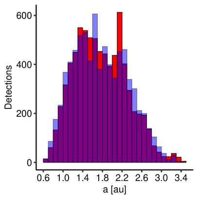
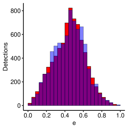
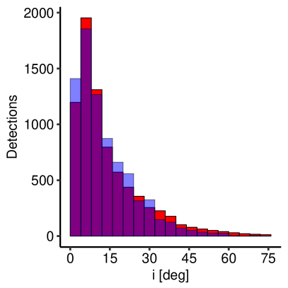
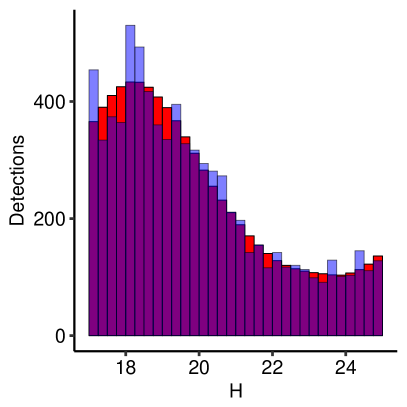
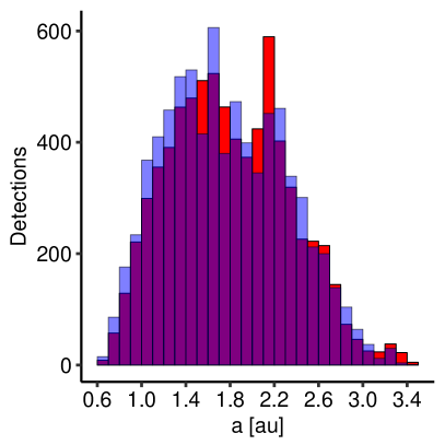
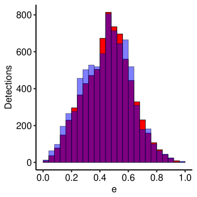
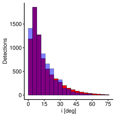
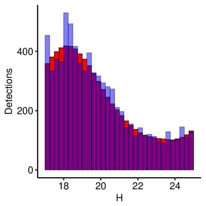
Figure 16: As Fig. 10 but using steady-state orbit distributions based on (top row) even-numbered and (bottom row) odd-numbered test asteroids.

6.4 Sensitivity to observational data

To assess the sensitivity of the model on the data set used for its calibration, we first divided the observations into two sets: those obtained by G96 and those obtained by 703. Then we constructed two models based on the data sets by using an approach otherwise identical to that described in Sect. 6.2. The marginal ($a$,$e$,$i$,$H$) distributions of the biased model, $\epsilon(a,e,i,H)\,N(a,e,i,H)$, compared to the observations show that both models accurately reproduce the observations from which they were derived (top and bottom panels in Fig. 17).

Prediction for 703 detections using model based on 703 detections

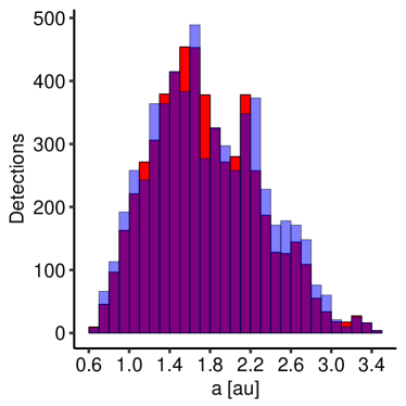
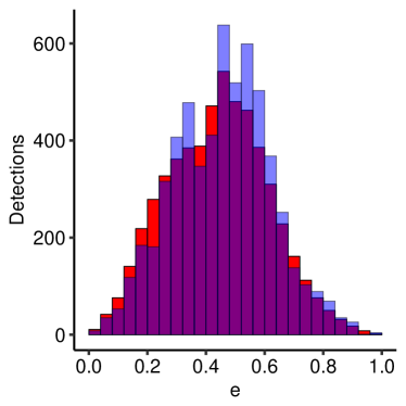
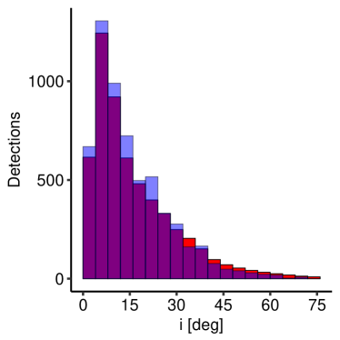
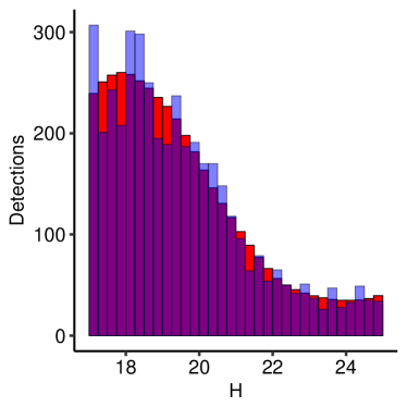
Prediction for 703 detections using model based on G96 detections

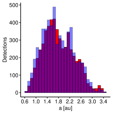
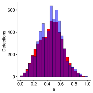
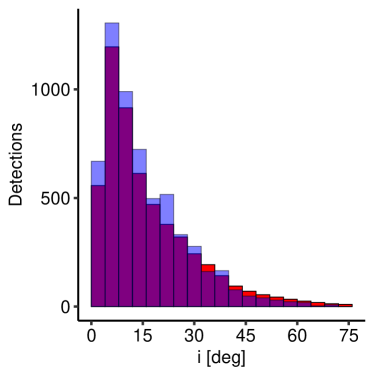
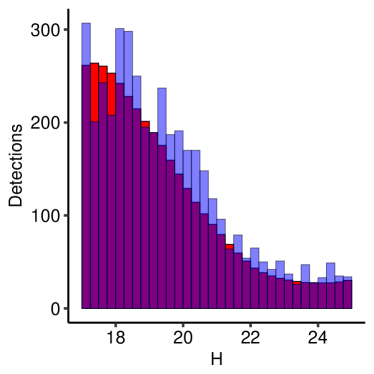
Prediction for G96 detections using model based on 703 detections

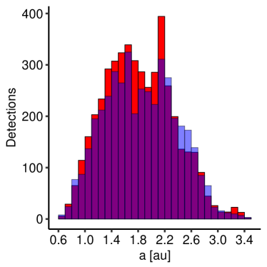
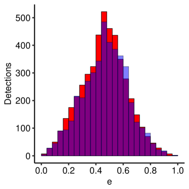
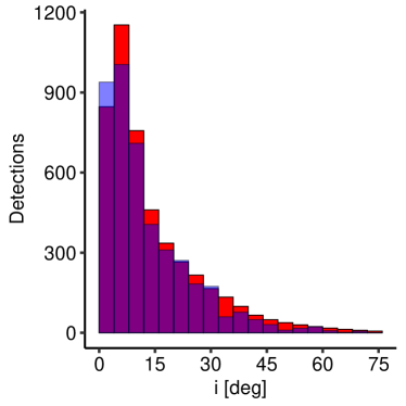
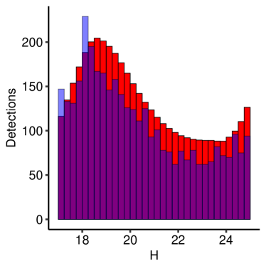
Prediction for G96 detections using model based on G96 detections

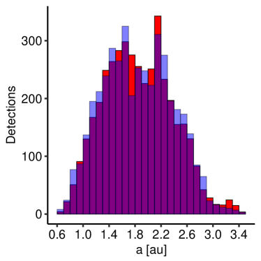
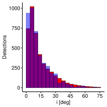
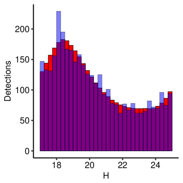
Figure 17: (Top row) Comparison between detections by 703 (blue; $n(a,e,i,H)$) and prediction based on the best-fit model using data by 703 (red; $\epsilon(a,e,i,H)\,N(a,e,i,H)$). (Upper middle row) Comparison between detections by 703 (blue) and prediction based on the best-fit model using data by G96 (red). The purple color indicates overlapping distributions. (Lower middle row) Comparison between detections by G96 (blue) and prediction based on the best-fit model using data by 703 (red). (Bottom row) Comparison between detections by G96 (blue) and prediction based on the best-fit model using data by G96 (red).

The critical test is then to predict, based on a model of G96 (703), what the other survey, 703 (G96), should have observed and compare this to the actual observations. For example, we should be able to detect problems with the input inclination distribution or the bias calculations, because the latitude distribution of NEO detections by 703 is wider than the latitude distribution by G96. It turns out that the shapes of the model distributions accurately match the observed distributions, but there are minor systematic offsets in the absolute scalings of the distributions (upper and lower middle panels in Fig. 17). The model based on detections by 703 only predicts about 9% too many detections by G96 whereas the model based on detections by G96 only predicts about 8% too few detections by 703. We interpret the discrepancy as a measure of the systematic uncertainty arising from the data set used for the modeling. Given that the models are completely independent of each other we consider the agreement satisfactory. In fact, none of the models described in the Introduction (except that of Granvik et al., 2016) have undergone a similar test of their predictive power. We also stress that the nominal model combines the 703 and G96 data sets and thus the systematic error is reduced from the less than 10% seen here.

We can take the test further by making predictions about the relative importance of different source regions as a function of $H$ (Fig. 18).

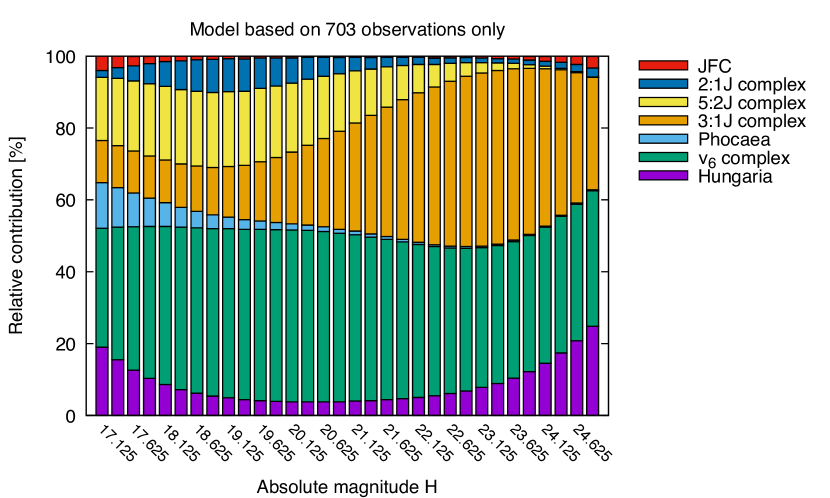
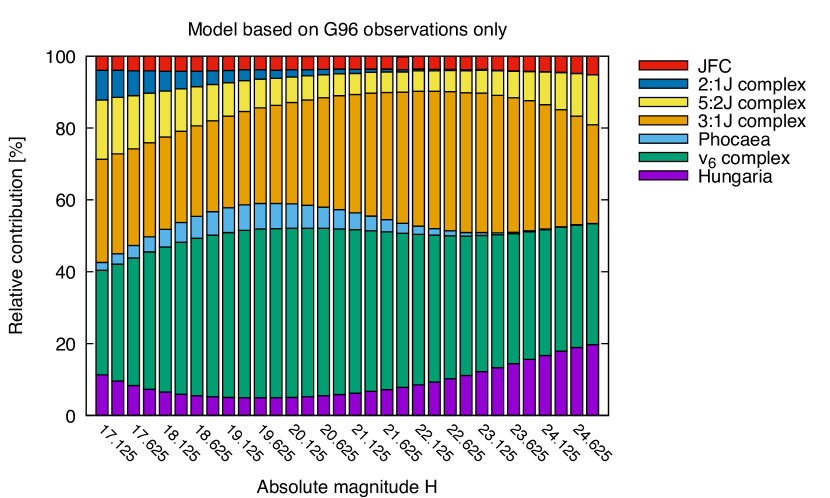
Figure 18: Relative importance of 7 different NEO source regions as a function of the absolute magnitude when the model is based only on (top) 703 and (bottom) G96.

The overall picture is consistent with our expectations in that the $\nu_{6}$ and 3:1J dominate both models. The difference for $\nu_{6}$ can largely be described by a constant such that the G96 model gives is a systematically smaller (by a few %-units) importance compared to the 703 model. The Hungarias show similar trends in both models, but the difference cannot be described as a simple systematic offset. Phocaeas show a clear difference in that their relative importance peaks at $H=17$ and $H\sim 19.5$ for 703 and G96, respectively. The common denominator for Phocaeas is that both models give them negligible importance for $H\gtrsim 23$. The 3:1J shows a similar overall shape with the importance peaking at $H\sim 23$ although the 703 model predicts a lesser importance at $H\lesssim 21$ compared to the G96 model. The G96 model gives a similar importance for 5:2J throughout the $H$ range whereas the 703 model gives a similar overall importance but limiting it to $H\lesssim 23$. The 2:1J has the opposite behaviour compared to the 5:2J in that its importance in the G96 model is primarily limited to $H\lesssim 21$ whereas its importance in the 703 model gives it a non-negligible importance throughout the $H$ range. Finally, the G96 model gives JFCs a nearly constant (a few %-units) importance throughout the $H$ range whereas the 703 model predicts that their importance is negligible for $19\lesssim H\lesssim 23.5$. We stress that this analysis does not account for uncertainties in model parameters which would make a difference in the relative importance more difficult to assess, in particular at large $H$ (see, e.g., Fig. 12).

6.5 Uniqueness

Although the similarity of the solutions based on different data sets suggest that the overall solution is stable, it does not directly imply that the parameters are unique. To study the uniqueness of the solution we computed a correlation matrix based on the parameters of the best-fit solution and the parameters of the 100 alternate solutions used for the uncertainty analysis described above. The correlation matrix shows that the 7 ERs and the penalty function are largely uncorrelated, but the parameters describing a single absolute-magnitude distribution or the penalty function are typically strongly correlated (Fig. 19). This suggests that the use of 7 ERs does not lead to a degenerate set of model parameters. Weak correlations are present between the Hungarias and the $\nu_{6}$ complex as well as between the $\nu_{6}$ and the 3:1J complexes. Both correlations are likely explained by partly overlapping orbit distributions. Somewhat surprisingly there is hardly any correlation between the two outer-MAB ERs — the 5:2J and 2:1J complexes. This suggests that they are truly independent components in the model.

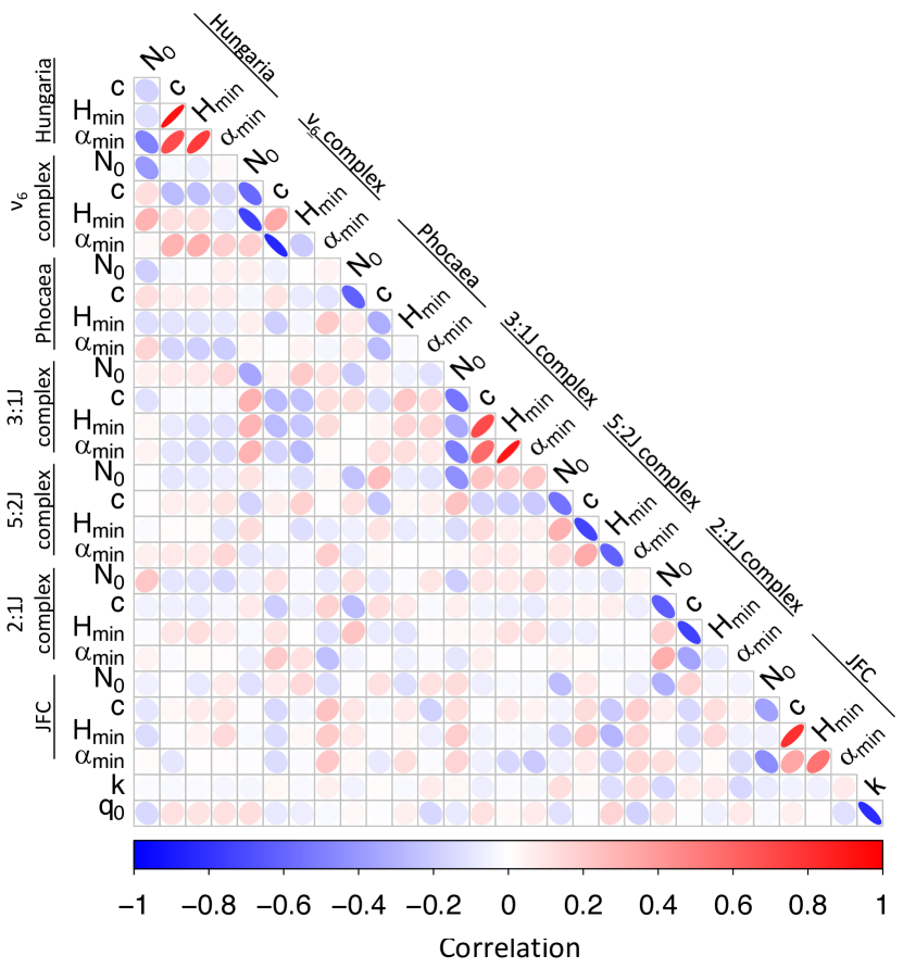
Figure 19: Correlations between model parameters.

A caveat with this analysis is that the samples of synthetic detections used for the alternative solutions are based on the steady-state orbit distributions and we used the same orbit distributions for fitting the model parameters. The small correlation between ERs might thus be explained by the fact that the synthetic orbits belong a priori to different ERs. We assume that the non-negligible overlap between the steady-state orbit distributions mitigate some or all of these concerns.

7 Discussion

7.1 Comparison to other population estimates

Our estimates for the incremental and cumulative NEO HFDs agree the most recent estimates published in the literature (Fig. 20 and Table 6). The relatively large uncertainties in the cumulative HFD are a reflection of the large uncertainties in the extrapolation to $H<17$.

Our estimates also both agree and disagree with older estimates such as that by Bottke et al. (2002a), for reasons we explain below. The estimate by Bottke et al. (2002a) is based on the work by Bottke et al. (2000). The ML technique used by both Bottke et al. (2000) and Bottke et al. (2002a) was able to characterize the slope of the NEO HFD where most of their data existed, namely between $17<H<22$. The HFD slope they found, $\gamma=0.35$, translates into a cumulative power-law size-distribution slope of -1.75. These values match our results and those of others (see, e.g., Harris and D’Abramo, 2015). The challenge for Bottke et al. (2000) was setting the absolute calibration of the HFD. Given that the slope of their HFD was likely robust, they decided to extend it so that it would coincide with the expected number of NEOs with $13<H<15$, a population that was much closer to completion. This latter population would serve as the calibration point for the model. At the time of the analysis by Bottke et al. (2000) there were 53 known NEOs in this $H$ range and they assumed a completeness ratio of 80% based on previous work by Rabinowitz et al. (2000). The expected number of NEOs with $13<H<15$ was therefore assumed to be about 66 whereas today we know that there are 50 such NEOs. The most likely explanation for the reduced number of known NEOs with $13<H<15$ over the past 17 years (from 53 to 50) is that the orbital and absolute-magnitude parameters of some asteroids have changed (i.e., improved) and they no longer fall into the category. We also now know that the HFD has a wavy shape with an inflection point existing near $H=17$, as shown in our work (Figs. 12 and 20). Thus, while the Bottke et al. (2002a) estimates for $H<18$ are on the low side but in statistical agreement with those provided here (i.e., $960\pm 120$ $H<18$ NEOs for Bottke et al. (2002a) vs. $\sim 1250$ here), their population estimate for $H<16$ is progressively too high.

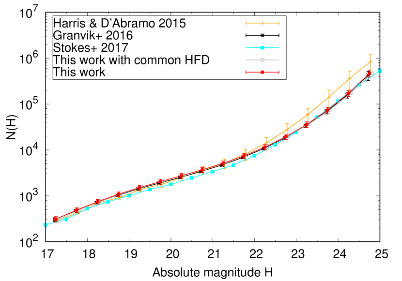
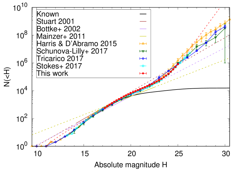
Figure 20: Our estimates for the debiased incremental (left) and cumulative (right) absolute-magnitude distributions for NEOs compared to published estimates. Extrapolations outside the validity regions for the different models are marked with dashed lines. The error bars for the model presented in this paper include both random and systematic uncertainties. The latter component is estimated to be 10% (Sects. 6.3 and 6.4).

Table 6: Incremental ($N(H)$) and cumulative ($N(<H)$) HFD in the fitted $H$ interval. The cumulative HFD has been scaled so that an extrapolation to smaller $H$ will predict 170 NEOs with $H<16$. The uncertainty estimates only account for the random component.

$H$	$N(H)$	$\sigma_{\mathrm{N(H),-}}$	$\sigma_{\mathrm{N(H),+}}$	$N(<H)$	$\sigma_{\mathrm{N(<H),-}}$	$\sigma_{\mathrm{N(<H),+}}$
17.125	1.378e+02	-5.900e+00	5.400e+00	5.695e+02	-4.640e+01	4.550e+01
17.375	1.739e+02	-5.700e+00	5.200e+00	7.434e+02	-5.110e+01	4.960e+01
17.625	2.187e+02	-6.000e+00	4.800e+00	9.620e+02	-5.590e+01	5.200e+01
17.875	2.728e+02	-5.800e+00	5.200e+00	1.235e+03	-5.900e+01	5.500e+01
18.125	3.370e+02	-6.800e+00	5.500e+00	1.572e+03	-6.100e+01	5.600e+01
18.375	4.113e+02	-7.100e+00	7.300e+00	1.983e+03	-6.100e+01	5.800e+01
18.625	4.960e+02	-8.600e+00	9.200e+00	2.479e+03	-6.300e+01	5.700e+01
18.875	5.914e+02	-1.080e+01	1.130e+01	3.071e+03	-6.600e+01	5.500e+01
19.125	6.979e+02	-1.300e+01	1.380e+01	3.768e+03	-7.100e+01	5.600e+01
19.375	8.165e+02	-1.680e+01	1.480e+01	4.585e+03	-7.800e+01	5.900e+01
19.625	9.490e+02	-2.140e+01	1.580e+01	5.534e+03	-8.600e+01	6.800e+01
19.875	1.098e+03	-2.300e+01	2.000e+01	6.632e+03	-9.600e+01	8.100e+01
20.125	1.269e+03	-2.800e+01	2.400e+01	7.901e+03	-1.140e+02	9.600e+01
20.375	1.467e+03	-3.300e+01	2.800e+01	9.368e+03	-1.390e+02	1.130e+02
20.625	1.701e+03	-4.000e+01	3.500e+01	1.107e+04	-1.800e+02	1.300e+02
20.875	1.985e+03	-4.700e+01	4.500e+01	1.305e+04	-2.100e+02	1.700e+02
21.125	2.334e+03	-5.600e+01	5.800e+01	1.539e+04	-2.500e+02	2.100e+02
21.375	2.775e+03	-7.000e+01	7.200e+01	1.816e+04	-2.900e+02	2.800e+02
21.625	3.343e+03	-9.500e+01	8.800e+01	2.151e+04	-3.700e+02	3.500e+02
21.875	4.088e+03	-1.210e+02	1.170e+02	2.559e+04	-4.400e+02	4.700e+02
22.125	5.088e+03	-1.570e+02	1.560e+02	3.068e+04	-5.800e+02	5.900e+02
22.375	6.453e+03	-2.020e+02	2.170e+02	3.713e+04	-7.500e+02	7.700e+02
22.625	8.358e+03	-2.850e+02	2.860e+02	4.549e+04	-1.010e+03	1.000e+03
22.875	1.107e+04	-3.900e+02	4.000e+02	5.656e+04	-1.360e+03	1.340e+03
23.125	1.502e+04	-5.700e+02	5.400e+02	7.158e+04	-1.850e+03	1.840e+03
23.375	2.090e+04	-8.400e+02	7.700e+02	9.247e+04	-2.630e+03	2.480e+03
23.625	2.988e+04	-1.270e+03	1.120e+03	1.224e+05	-3.800e+03	3.400e+03
23.875	4.399e+04	-2.030e+03	1.690e+03	1.663e+05	-5.400e+03	5.100e+03
24.125	6.685e+04	-3.280e+03	2.900e+03	2.332e+05	-8.400e+03	7.500e+03
24.375	1.051e+05	-5.490e+03	5.600e+03	3.383e+05	-1.350e+04	1.210e+04
24.625	1.717e+05	-1.040e+04	1.160e+04	5.101e+05	-2.220e+04	2.290e+04
24.875	2.923e+05	-1.890e+04	2.920e+04	8.024e+05	-4.240e+04	4.790e+04

We confirm that the slope of the HFD reaches a minimum at $H\sim 20$ (Fig. 20) and, since it is also seen for different ERs (Fig. 12), conclude that it cannot be caused by the combination of differently-sloped and power-law shaped HFDs. Instead the wavy shape is likely related to the nature of how asteroids disrupt (see, e.g., Durda et al., 1998; Bottke et al., 2005, 2015a). Small asteroids are considered part of the “strength-scaling” regime, where the fragmentation of the target body is governed by its tensile strength, while large asteroids are considered part of the “gravity scaling” regime, where fragmentation is controlled by the self-gravity of the target. Laboratory experiments and hydrocode modeling work suggest the transition between the two regimes occurs near 100–200-meter-diameter bodies, which corresponds to $21\lesssim H\lesssim 22$ assuming a geometric albedo $p_{V}=0.14$ (smaller $H$ for higher albedos). It has also been suggested that it is caused by the transition from the strong ”monolithic” structures to the weaker ”rubble-pile” structures held together by gravitational forces, as proposed by Harris and D’Abramo (2015). Objects with $21\lesssim H\lesssim 22$ fall in between these categories and are more easily disrupted than larger or smaller objects. An alternative explanation is that the physical size distribution can be described by a powerlaw but the albedo distribution varies as a function of size. This could effectively lead to a dip in the HFD. However, this would probably require an unrealistically large change in the average albedo as a function of $H$ (Werner et al., 2002).

Our results for the orbital distributions also mostly agree with results found in the literature. For large NEOs ($H<18.5$) we can compare our debiased marginal ($a$,$e$,$i$) distributions with those by Stuart (2001) and Tricarico (2017). Whereas we find a good agreement for the $a$ and $e$ distributions we do not confirm the strong peak in the inclination distribution at $20^{\circ}\lesssim i\lesssim 30^{\circ}$ predicted by Stuart (2001). However, we do predict that the distribution has a lesser bump at $20^{\circ}\lesssim i\lesssim 40^{\circ}$ (Fig. 21) in agreement with Tricarico (2017). We also note that the inclination distribution for the known NEOs shows a similar bump suggesting that we are looking at a real phenomenon, although the exact shape of the bump is sensitive to the bin size. The bump was not predicted by the model by Bottke et al. (2002a), because it is caused by the Hungarias and Phocaeas and those ERs were not included in their model.

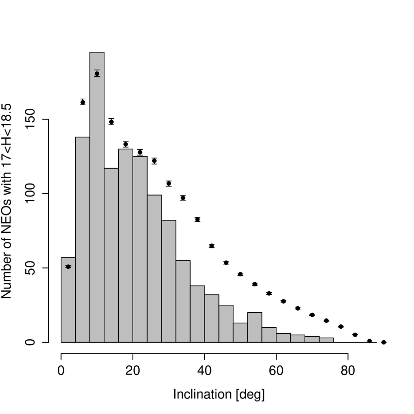
Figure 21: Our estimate for the debiased inclination distribution for NEOs with $17<H<18.5$ compared to currently known NEOs in the same $H$ range (ASTORB 2018-01-30). The uncertainties were computed as single-sided RMS estimates with respect to the nominal model by utilizing 100 alternative models as explained in Sect. 6.2. The error bars do not account for systematic uncertainties.

For NEOs with $22<H(<25)$ there are no debiased orbit models available and hence we cannot compare our results to the literature.

7.2 Extrapolation to larger and smaller NEOs

Although the calibration of our model is limited to $17<H<25$, we may occasionally want to extrapolate to larger and/or smaller objects. The limitation of such extrapolations is that the orbit distributions, and hence the relative ratios between the ERs, are fixed to either $H=17$ or $H=25$, depending on if the extrapolation is towards larger or smaller NEOs, respectively.

When extrapolating to larger NEOs, that is, to those with $H<17$, we use a power-law function for the extrapolation and obtain the slope from our estimate for $17<H<17.5$ NEOs. We also rescale the extrapolation so that the cumulative number of NEOs with $H<16$ coincides with the current number of known NEOs, that is, 170. An extrapolation to smaller $H$ values would predict 207 $H<16$ NEOs without the rescaling. The extrapolation predicts a few too many NEOs at $12\lesssim H\lesssim 15$ but we think that the agreement with the known population is still reasonable for most purposes (Fig. 20 right). Considering that the NEO inventory is virtually complete for $H<17$ one may alternatively choose to simply append the known population for the $H<17$ part.

An issue, however, is that many larger MBOs escape the MAB out of the ”forest” of weak resonances in the inner MAB (e.g., Nesvorný and Morbidelli, 1998; Morbidelli and Nesvorný, 1999). The bigger they are, the more difficult time they will have reaching one of the main NEO sources via Yarkovsky drift (Bottke et al., 2006). As discussed above, a potential problem with our model for large asteroids is that the test asteroids we have chosen to represent them have such high Yarkovsky semimajor axis drift rates that most will jump over these weak resonances. Given that most large NEOs are known, this does not present a problem for our NEO model per se, but a future NEO model wanting to make predictions about, e.g., planetary impacts by large NEOs will need to worry about getting the dynamics right for these bodies. In addition, Nesvorný and Roig (2018) have recently shown that the large end of the NEO population does not appear to be in steady-state which is the assumption behind the modeling carried out here. Hence it is not surprising that an extrapolation of the model described here cannot accurately reproduce the large end of the NEO HFD.

When extrapolating to smaller NEOs, that is, those with $H>25$ we can estimate the slope from our model for $24.5<H<25$ and use that for the extrapolation. However, that approach does not lead to a good agreement with the HFD by Harris and D’Abramo (2015) for $H\geq 27$. When converted to the rate of Earth impacts, Harris and D’Abramo (2015) is in reasonable agreement with the observed rate of impacts on the Earth (Brown et al., 2002, 2013). A more accurate extrapolation, that is, one that is more in line with the literature, can be obtained by using a slope found by others (e.g., Brown et al., 2002, 2013) for $H>25$.

7.3 Completeness of the current inventory of NEOs

The surveys have so far found 905 NEOs with the estimated $D>1\,\mathrm{km}$ ($H<17.75$; ASTORB 2018-01-30). Assuming that the $H<16$ population is essentially complete and currently includes 170 NEOs, we predict a population of $962^{+52}_{-56}$ for NEOs with $H<17.75$ (the uncertainty estimates only account for the random component; Fig. 20 right and Table 6). This implies that about 94% of all NEOs with $H<17.75$ have been found to date.

The orbits of the undiscovered large NEOs are characterized by high inclinations and relatively small semimajor axes (Fig. 22). NEOs with such orbital characteristics are challenging to detected because they can have relatively long synodic periods and they may be bright enough only at perihelion when they can be in the southern hemisphere. Finding these NEOs thus require longer surveys carried out (also) in the southern hemisphere and/or larger apertures. An example of such a challenging NEO to discover is 2017 MK₈ ($a=2.51\,\mathrm{au}$, $e=0.67$, $i=31.6^{\circ}$, $H=16.5$) which was discovered by Pan-STARRS as recently as in June 2017. This particular object crosses the ecliptic approximately at perihelion when inside the Earth’s orbit and at aphelion (at a distance of about $4\,\mathrm{au}$ from the Sun).

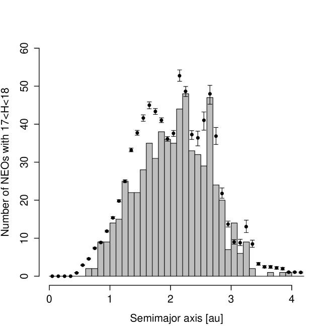
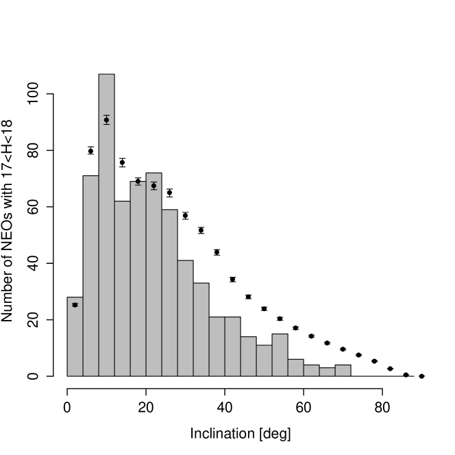
Figure 22: Known (ASTORB 2018-01-30; histogram) and predicted (dot with errorbars) marginal orbital-element distributions for NEOs with $17<H<18$. The uncertainties were computed as single-sided RMS estimates with respect to the nominal model by utilizing 100 alternative models as explained in Sect. 6.2. The error bars do not account for systematic uncertainties.

For smaller objects with $17<H<20$ the need for improved instrumentation becomes even more urgent as in addition to high-$i$ NEOs also large-$a$ NEOs remain undiscovered (Fig. 23). Smaller and more distant NEOs are difficult to detect due to their greater average distances from the observer and higher rates of motion when close to the Earth.

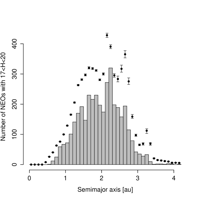
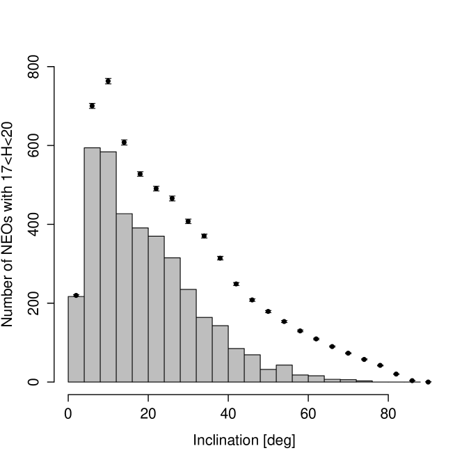
Figure 23: Known (ASTORB 2018-01-30; histogram) and predicted (dot with errorbars) marginal orbital-element distributions for NEOs with $17<H<20$. The uncertainties were computed as single-sided RMS estimates with respect to the nominal model by utilizing 100 alternative models as explained in Sect. 6.2. The error bars do not account for systematic uncertainties.

The main difference between the orbits of undiscovered small (Fig. 23) and large (Fig. 22) NEOs is that the former are more notably characterized by large eccentricities. As most of the known high-inclination NEOs have been discovered prior to, e.g., Pan-STARRS, which is the most prolific survey telescope currently operating, we find it unlikely that the remaining large, high-inclination NEOs would be discovered in the next decade without substantial improvements in observation strategy and/or instrumentation.

7.4 NEO flux from different ERs

The relative flux of asteroids and comets into the NEO population as a function of ER is strongly size dependent (Table 4). The number-weighted flux of NEOs in general ($17<H<25$) is dominated by inner-MAB ERs whereas the number-weighted flux of $D>100\,\mathrm{m}$ ($17<H<22$) NEOs is dominated by outer-MAB ERs. The domination of outer-MAB ERs for large NEOs has been seen before (Bottke et al., 2002a) but the change to domination by inner-MAB ERs for smaller NEOs has not been shown before.

Recently Granvik et al. (2017) estimated the relative flux of asteroids into the NEO population from different ERs through direct integrations of MBOs. They found a good agreement with (Bottke et al., 2002a) for $D=3\,\mathrm{km}$ objects but unfortunately the smallest diameter considered, $D=0.1\,\mathrm{km}$ ($H\sim 22.7$), is still fairly close to the ”large” group and hence they do not see the transition to inner-MAB domination. Instead the relative fluxes for all the diameters considered ($0.1\,\mathrm{km}$–$3.0\,\mathrm{km}$) are statistically indistinguishable. Focusing on the large group only we find that the flux through the 5:2J complex is the highest (Table 4) followed by the 3:1J, 2:1J and $\nu_{6}$ complexes and Phocaeas and Hungarias in descending order. The relative numbers are remarkably close to those predicted by Granvik et al. (2017) for $D=0.1\,\mathrm{km}$ asteroids through direct orbital integrations. The largest relative difference between our estimates and those by Granvik et al. (2017) is found for Hungarias in that our estimate is a factor of about three higher.

7.5 NEAs on retrograde orbits

We find that the fraction of retrograde objects ranges from about 1% to 2.5% depending on the range in $H$ magnitude and the main ERs are the 3:1J complex and JFCs (Fig. 24). In particular, when extrapolating our model down to $H=15$ it predicts that there are 0.5 (3.5) NEAs on retrograde orbits with $15<H\leq 16$ ($15<H\leq 18$). Greenstreet et al. (2012b) suggest that the NEO (343158) 2009 HC₈₂ is of asteroidal origin despite its retrograde orbit. The absolute magnitude for (343158) is 16.1 according to the MPC which agrees with our predicted number of NEAs on retrograde orbits assuming a 100% completeness for $H\lesssim 16$ NEAs and suggests that (343158) is the largest NEA on a retrograde orbit. Based on the new model we predict that there are still 2–3 $H<18$ NEAs on retrograde orbits left to be discovered. The fraction of unknown retrograde $H<18$ NEOs may appear surprisingly high considering that about 90% of all prograde NEOs in the same $H$ range have been discovered. We note, however, that the undiscovered large retrograde NEOs likely reside on nearly polar orbits that make them hard to discover (cf. Fig 22).

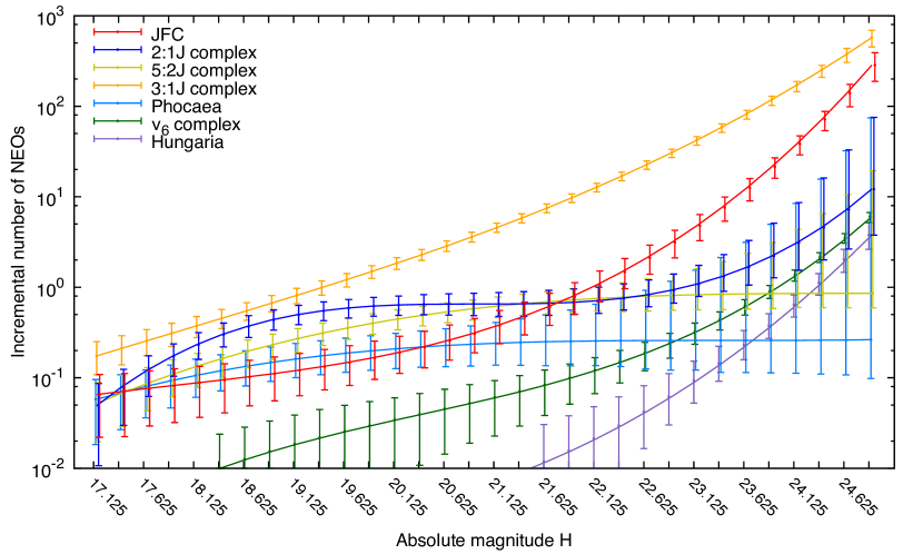
Figure 24: Debiased, incremental absolute-magnitude distributions for NEOs on retrograde orbits from different ERs.

The mechanism producing NEAs on retrograde orbits is primarily related to the 3:1J MMR as suggested by Greenstreet et al. (2012b) because most NEAs evolve to $i>90^{\circ}$ orbits when their $a\sim 2.5\,\mathrm{au}$ (Fig. 25). Note that (343158) 2009 HC₈₂ has $a\sim 2.53\,\mathrm{au}$ which puts it in the 3:1J MMR.

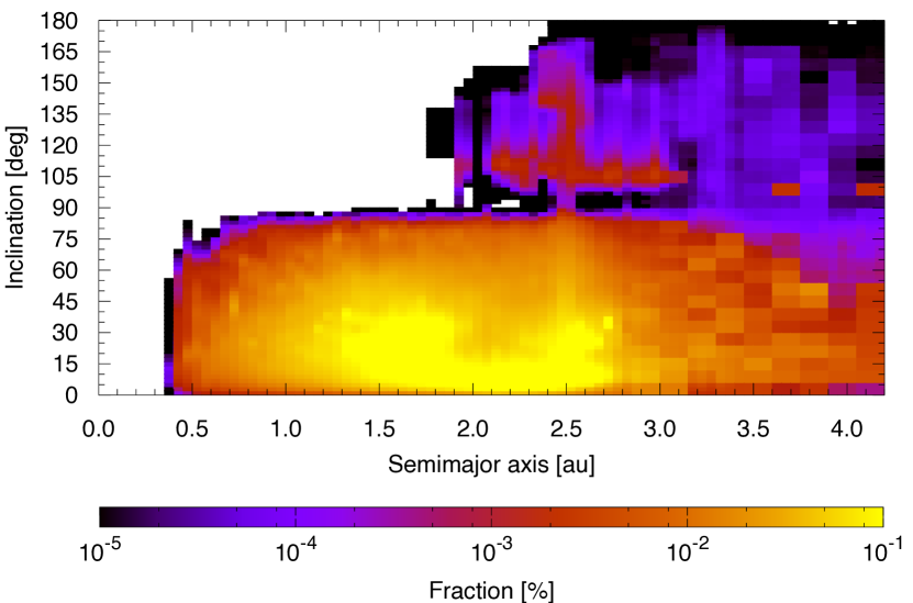
Figure 25: NEO steady-state ($a,i$) distribution for $17<H<25$.

7.6 Collision rate on terrestrial planets

In order to compute the collision probabilities of NEOs with Mercury, Venus and the Earth (we neglect Mars because the latter is also bombarded by asteroids which have $q>1.3$ au, not included in our model) we adopted the following procedure. For each cell in orbital space $(a,e,i)$ considered in our NEO model, we have computed the collision probability $P_{\rm col}(a,e,i)$ and impact velocity $v_{\rm col}(a,e,i)$ with the considered planet, using an Öpik-like code described in Vokrouhlický et al. (2012) and Pokorný and Vokrouhlický (2013). This code is superior to the one originally described in Wetherill (1967), because it accounts for the fact that the eccentricity and the inclination of an object oscillate in a coupled manner together with the precession of the argument of perihelion $\omega$. This oscillation is prominent when the $z$-component of the angular momentum is small (i.e., the well-known Lidov-Kozai oscillations: Lidov, 1962; Kozai, 1962). Thus, the code requires that the values of $a,e,i$ of the projectile be specified as well as the corresponding value of $\omega$. Because $\omega$ was not tracked in our model, for each cell we considered 10 particles, each with the ($a,e,i$) values corresponding to the center of the cell, and values of $\omega$ ranging from 0 to 90 degrees, with steps of 10 degrees. For simplicity we have assumed that each planet has a null inclination relative to the reference plane, but we used its actual orbital eccentricity. For each of these 10 particles, the code outputs a different collision probability $P_{(a,e,i)}(\omega)$ and velocity $v_{(a,e,i)}(\omega)$. The collision probability and velocity for objects in the cell $P_{\rm col}(a,e,i),v_{\rm col}(a,e,i)$ are computed as the averages of these quantities. In computing the averages we recognize the symmetry of the $\omega$-induced dynamics relative to the axes $\sin{\omega}=0$ and $\cos{\omega}=0$ and therefore the values of $P_{(a,e,i)},v_{(a,e,i)}$ for $\omega\neq 0,90^{\circ}$ are considered twice while $P_{(a,e,i)}(0),v_{(a,e,i)}(0),P_{(a,e,i)}(90),v_{(a,e,i)}(90)$ only once. Moreover, in computing the average of $v_{(a,e,i)}$ we weight with $P_{(a,e,i)}$.

Once the values $P_{\rm col}(a,e,i),v_{\rm col}(a,e,i)$ are computed for each cell, the total collision probability with the planet (impacts per year) is computed as

$$P_{\rm tot}=R_{p}^{2}\sum_{a,e,i}N_{\rm tot}(a,e,i)P_{\rm col}(a,e,i)\left(1+\frac{v_{\rm esc}^{2}}{v_{\rm col}^{2}(a,e,i)}\right)\,$$ (13)

where $R_{p}$ is the radius of the planet, $v_{\rm esc}$ is the escape velocity for its surface, and $N_{\rm tot}(a,e,i)=\sum_{H}N(a,e,i,H)$ is the number of asteroids in each orbital-magnitude cell of our model. Note that the term in parentheses on the right hand side implies that our collision probability calculation accounts for gravitational focusing.

The result is illustrated in Fig. 26 in a cumulative form (number of impacts per year on a planet for impactors brighter than a given magnitude $H$). The cumulative rate of Earth impacts by NEOs with $H<25$ is approximately once per millenium (Fig. 26). The results are in very good agreement with those reported in Morbidelli et al. (2002) (Table 5) for $H<17.3$, $H<19.0$, and $H<20.6$. While our nominal rate is about 3 times smaller than another contemporary estimate for $H<25$ (Harris and D’Abramo, 2015), we stress that this difference is explained by the difference in the HFDs rather than in the calculation of the impact rate. The estimates overlap at the 1$\sigma$ level when accounting for the uncertainties of the HFDs (Fig. 20).

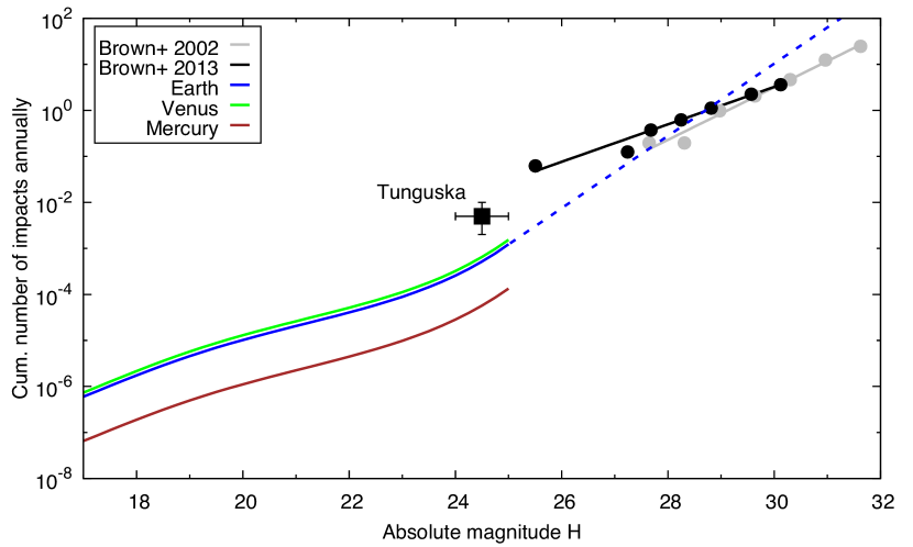
Figure 26: Cumulative annual rate of impacts on terrestrial planets predicted by our model and observed rate of bolides on the Earth (Brown et al., 2013, 2002). The dashed line marks a linear extrapolation based on our prediction for the slope at $24.5<H<25$. The conversion from bolide energy to absolute magnitude $H$ assumes a spherical shape, a bulk density of $3,000\,\mathrm{kg}\,\mathrm{m}^{-3}$, an average impact speed of $20.3\,\mathrm{km}\,\mathrm{s}^{-1}$, and a geometric albedo of 0.14. The error bars (and the nominal value) for the Tunguska event are approximate assuming that similar events happen every 100–500 years and that the diameter of the impactor is about 50 meters with the geometric albedo ranging from 0.05 to 0.25.

A linear extrapolation of the cumulative impact rate in the ($H,\log{N(<H)}$) space reproduces the observed rate of decameter-scale and smaller asteroids and meteoroids to within an order of magnitude (Fig. 26; Brown et al., 2013, 2002). A better match to the observed rate of bolide impacts would require a steeper slope at $24\lesssim H\lesssim 26$. If the higher-than-expected rate of large bolides is more than just a statistical anomaly, the extrapolation suggests that the NEO HFD has a bump at $24\lesssim H\lesssim 28$ that has not been predicted by NEO models so far to the best of our knowledge. However, one has to bear in mind that the largest bolides are single events and therefore their frequency is uncertain (see, e.g., Boslough et al., 2015).

The impact-flux ratios are fairly stable throughout the considered $H$ range (Fig. 27). The uncertainty on these estimates is driven by the uncertainty in the orbit distribution and HFD, and not more than about 10% based on the discussion in Sect. 6.2. Our total impact flux ratio for Venus and Earth ($\sim 1.2$) agrees with Vokrouhlický et al. (2017) whereas our estimates for the impact flux ratios per surface area for Venus and Earth ($\sim 1.4$) and Mercury and Earth ($\sim 0.75$) do not agree with the ones reported in Greenstreet et al. (2012a) but are about 20% higher and 40% lower, respectively. Given the rather trivial conversion from the total impact-flux ratio to the impact-flux ratio per surface area it seems that also Vokrouhlický et al. (2017) and Greenstreet et al. (2012a) are at odds with each other.

Figure 27: Total and per-surface-area impact-flux ratios Venus/Earth and Mercury/Earth as a function of impactor $H$ magnitude. These ratios do not account for the destruction of asteroids at small $q$ which changes all ratios as a function of $H$ (Table 3).

Fig. 28 shows the relative contribution of each source to the terrestrial impact rate. About 80% of the impacts come from the $\nu_{6}$ SR. Thus, the inner MAB is the predominant source of impactors. Given that the population of primitive asteroids in the inner MAB is more than 20% of the total (DeMeo and Carry, 2014), this implies that most of the primitive NEOs also come from the $\nu_{6}$ SR. This is in agreement with the results of Campins et al. (2010, 2013) and Bottke et al. (2015b) who investigated the most likely origin of specific primitive NEOs.

Figure 28: Source regions for Earth impactors with $H<20$.

The production rate of $D>20\,\mathrm{km}$ craters across the Earth’s surface over the last 100 Myr or so has been estimated from lunar craters to be $2.5(\pm 1.1)\times 10^{-15}$ km^-2 yr^-1 and from terrestrial craters to be $2.8(\pm 1.1)\times 10^{-15}$ km^-2 yr^-1 (Mazrouei et al., 2018). Hughes (2000), using a different method, estimated the production rate of $D>22$ km craters across the Earth’s surface over the last 125 Myr to be $3.0(\pm 0.3)\times 10^{-15}$ km^-2 yr^-1. We can compare these values to predictions from our model, assuming that the scaling relationship to turn projectiles into terrestrial craters is a factor of 20 (see, e.g., Melosh, 1989). Combining our collision probability results with 962 km-sized NEOs ($H<17.75$), 58% which are on Earth crossing orbits, yields a model production rate for terrestrial $D>20$ km craters of $2.4\times 10^{-15}$ km^-2 yr^-1. This value is in statistical agreement with the estimates from Mazrouei et al. (2018) but slightly outside the error bars for Hughes (2000). The difference for the latter, however, could simply suggest we need to slightly modify our crater scaling laws (see, e.g., Bottke et al., 2016).

7.7 ESA NEO service and access to realizations of the model

The model and tools for survey simulations have been made available by ESA through their Space Situational Awareness website dedicated to NEOs. The tool for generating a realization of the model produces a distribution of orbital elements and absolute magnitudes in the range $17<H<25$ by default, but the user has the option to extrapolate to larger and/or smaller $H$ magnitudes. The user may either define his/her own slope for the HFD outside the default range or use one of the predefined slopes. To improve the statistics it is also possible to provide a scaling factor, which is unity for the nominal model and, e.g., 10 for a population 10 times larger than the nominal population for the same $H$ range.

To simplify access to the model, we also provide direct access to a realization of the nominal model for the default $H$ range. The flat file contains orbital elements and absolute magnitudes ($a$,$e$,$i$,$H$) for 802,000 NEOs with $a<4.2\,\mathrm{au}$ and $17<H<25$.

8 Conclusions

We have developed a four-dimensional model describing the debiased NEO orbit ($a,e,i$) and absolute-magnitude ($H$) distributions. The free parameters in our modeling approach describe $H$ distributions for asteroids and comets that entered the NEO region through 7 different ERs in the MAB or the cometary region. Our modeling methodology, tools and results have been carefully vetted through comparing independent predictions of NEO detections and actual detections by CSS’s stations 703 and G96 — to the best of our knowledge such detailed and independent quality-control measures have never been employed in the past during the development of NEO population models.

We see statistically-significant differences in the shapes of the fitted $H$ distributions for the different ERs. The shapes range from almost flat (Phocaeas and the 5:2J complex) to simple power-law (3:1J complex) to increasing slope (Hungarias and JFCs) to waves (the $\nu_{6}$ and 2:1J complexes). Understanding the reason behind these differences is challenging because the shapes of the $H$ distributions are a convolution of the dynamical mechanisms (such as Yarkovsky and YORP) that replenish the NEO population and the asteroids’ material properties.

The fitted $H$ distributions also provide direct estimates for the absolute contributions of NEOs from 7 different ERs. Our predicted fractional contributions agree with previous estimates by Bottke et al. (2002a) in the sense that the $\nu_{6}$ and 3:1J complexes are the most significant ERs. Most NEOs thus originate in the inner MAB. The outer MAB and the JFCs contribute only about 10–25% of the steady-state NEO population depending on $H$. The JFCs contribution alone is about 2–10% depending on $H$. In addition, our model shows for the first time that the Hungaria group is an important source for NEOs whereas the Phocaea group is a less important source. Combined these high-inclination groups solve the controversy as to (initially) the existence (Stuart, 2001) and (later) the origin of high-inclination NEOs.

Our estimate for the number of NEOs on retrograde orbits is in agreement with Greenstreet et al. (2012a, b). These retrograde NEOs are dominated by the asteroids from the 3:1J complex with a lesser contribution from JFCs. This results in a substantially different overall shape for the HFD compared to NEOs on prograde orbits. We also note that these results clearly imply that the 3:1J MMR plays a key role in the production of NEOs on retrograde orbits.

Our results for the debiased marginal $a$, $e$, $i$ and $H$ distributions for large NEOs generally agree with the most recent literature with the exception that the inclination distribution is weakly bimodal due to the contribution from the Hungaria group. Although the main features of the orbit distribution are fairly stable across the considered $H$ range due to the substantial contribution from $\nu_{6}$ and 3:1J complexes across $H$, there is a clear but complex fluctuation with $H$ on top of that. Most of the fluctuation is explained by variation in contributions from the 5:2J complex and the Hungarias. In particular, the contribution from Hungarias is largest at the smallest sizes whereas the opposite is true for the 5:2J complex.

The relative fractions of Amors, Apollos, Atens, Atiras, and Vatiras are fairly insensitive to $H$. Our estimates for the relative fractions for $17<H<25$ are markedly different compared to the estimates by both Greenstreet et al. (2012a) and Bottke et al. (2002a) for $H<18$. A difference with respect to both Greenstreet et al. (2012a) and Bottke et al. (2002a) suggests that statistical uncertainties in the ER-specific steady-state orbit distributions that are used for the orbit models is not the culprit. Instead we think that the difference is driven by improved estimates of the relative contributions from different ERs.

Based on our NEO model and Öpik-like impact analysis we find a good agreement to earlier estimate for the impact rate on terrestrial planets in the literature for large NEOs. For smaller NEOs we can compare a linear extrapolation of our model to smaller sizes with the observed rate of bolides on the Earth. The agreement is reasonably good apart for $24<H<28$ where the frequency of Tunguska-sized impacts remains an unsettled issue. We also find a good agreement between our prediction and lunar cratering records.

Finally, our work suggests that the NEO population is in a steady state, at least for $H\geq 17$, because our model is based on that assumption and it accurately reproduces the observed population.

Acknowlegdements

We thank Pasquale Tricarico and Alan Harris for their detailed reviews that helped improve the manuscript. M.G. was funded by grants 137853 and 299543 from the Academy of Finland, and D.V. by grant GA13-01308S of the Czech Science Foundation. W.F.B. thanks NASA’s Near Earth Object Observation program for supporting his work in this project. We acknowledge support by ESA via contract AO/1-7015/11/NL/LvH (SGNEOP). CSC — IT Centre for Science, Finland, the Finnish Grid Infrastructure and the mesocentre SIGAMM at Observatoire de la Côte d’Azur provided computational resources.

References

References

- Abell et al. (2015) Abell, P.A., Barbee, B.W., Chodas, P.W., Kawaguchi, J., Landis, R.R., Mazanek, D.D., Michel, P., 2015. Human Exploration of Near-Earth Asteroids, in: Michel, P., DeMeo, F.E., Bottke, W.F. (Eds.), Asteroids IV, pp. 855–880.
- Akaike (1974) Akaike, H., 1974. A new look at the statistical model identification. IEEE Transactions on Automatic Control 19, 716–723.
- Binzel et al. (2015) Binzel, R.P., Reddy, V., Dunn, T.L., 2015. The Near-Earth Object Population: Connections to Comets, Main-Belt Asteroids, and Meteorites, in: Michel, P., DeMeo, F.E., Bottke, W.F. (Eds.), Asteroids IV, pp. 243–256.
- Boslough et al. (2015) Boslough, M., Brown, P., Harris, A., 2015. Updated population and risk assessment for airbursts from near-Earth objects (NEOs), in: 2015 IEEE Aerospace Conference, pp. 1–12.
- Bottke et al. (2015a) Bottke, W.F., Brož, M., O’Brien, D.P., Campo Bagatin, A., Morbidelli, A., Marchi, S., 2015a. The Collisional Evolution of the Main Asteroid Belt, in: Michel, P., DeMeo, F.E., Bottke, W.F. (Eds.), Asteroids IV, pp. 701–724.
- Bottke et al. (2005) Bottke, W.F., Durda, D.D., Nesvorný, D., Jedicke, R., Morbidelli, A., Vokrouhlický, D., Levison, H.F., 2005. Linking the collisional history of the main asteroid belt to its dynamical excitation and depletion. Icarus 179, 63–94.
- Bottke et al. (2000) Bottke, W.F., Jedicke, R., Morbidelli, A., Petit, J.M., Gladman, B., 2000. Understanding the Distribution of Near-Earth Asteroids. Science 288, 2190–2194.
- Bottke et al. (2002a) Bottke, W.F., Morbidelli, A., Jedicke, R., Petit, J.M., Levison, H.F., Michel, P., Metcalfe, T.S., 2002a. Debiased Orbital and Absolute Magnitude Distribution of the Near-Earth Objects. Icarus 156, 399–433.
- Bottke et al. (2016) Bottke, W.F., Vokrouhlický, D., Ghent, B., Mazrouei, S., Robbins, S., Marchi, S., 2016. On Asteroid Impacts, Crater Scaling Laws, and a Proposed Younger Surface Age for Venus, in: Proceedings of the Lunar and Planetary Science Conference, LPI, Houston, TX, USA. p. 2036.
- Bottke et al. (2002b) Bottke, W.F., Vokrouhlický, D., Rubincam, D.P., Broz, M., 2002b. The Effect of Yarkovsky Thermal Forces on the Dynamical Evolution of Asteroids and Meteoroids, in: Bottke, W., Cellino, A., Paolicchi, P., Binzel, R.P. (Eds.), Asteroids III. University of Arizona Press, pp. 395–408.
- Bottke et al. (2006) Bottke, W.F., Vokrouhlický, D., Rubincam, D.P., Nesvorný, D., 2006. The Yarkovsky and Yorp Effects: Implications for Asteroid Dynamics. Annual Review of Earth and Planetary Sciences 34, 157–191.
- Bottke et al. (2015b) Bottke, W.F., Vokrouhlický, D., Walsh, K.J., Delbo, M., Michel, P., Lauretta, D.S., Campins, H., Connolly, H.C., Scheeres, D.J., Chelsey, S.R., 2015b. In search of the source of asteroid (101955) Bennu: Applications of the stochastic YORP model. Icarus 247, 191–217.
- Brasser and Morbidelli (2013) Brasser, R., Morbidelli, A., 2013. Oort cloud and Scattered Disc formation during a late dynamical instability in the Solar System. Icarus 225, 40–49.
- Brown et al. (2002) Brown, P., Spalding, R.E., ReVelle, D.O., Tagliaferri, E., Worden, S.P., 2002. The flux of small near-Earth objects colliding with the Earth. Nature 420, 294–296.
- Brown et al. (2013) Brown, P.G., Assink, J.D., Astiz, L., Blaauw, R., Boslough, M.B., Borovička, J., Brachet, N., Brown, D., Campbell-Brown, M., Ceranna, L., Cooke, W., de Groot-Hedlin, C., Drob, D.P., Edwards, W., Evers, L.G., Garces, M., Gill, J., Hedlin, M., Kingery, A., Laske, G., Le Pichon, A., Mialle, P., Moser, D.E., Saffer, A., Silber, E., Smets, P., Spalding, R.E., Spurný, P., Tagliaferri, E., Uren, D., Weryk, R.J., Whitaker, R., Krzeminski, Z., 2013. A 500-kiloton airburst over Chelyabinsk and an enhanced hazard from small impactors. Nature 503, 238–241.
- Burnham and Anderson (2002) Burnham, K.P., Anderson, D.R., 2002. Model Selection and Multimodel Inference A Practical Information-Theoretic Approach. Springer, New York. 2nd edition.
- Campins et al. (2013) Campins, H., de León, J., Morbidelli, A., Licandro, J., Gayon-Markt, J., Delbo, M., Michel, P., 2013. The Origin of Asteroid 162173 (1999 JU3). AJ 146, 26.
- Campins et al. (2010) Campins, H., Morbidelli, A., Tsiganis, K., de León, J., Licandro, J., Lauretta, D., 2010. The Origin of Asteroid 101955 (1999 RQ36). ApJ 721, L53–L57.
- Chesley et al. (2003) Chesley, S.R., Ostro, S.J., Vokrouhlický, D., Čapek, D., Giorgini, J.D., Nolan, M.C., Margot, J.L., Hine, A.A., Benner, L.A.M., Chamberlin, A.B., 2003. Direct Detection of the Yarkovsky Effect by Radar Ranging to Asteroid 6489 Golevka. Science 302, 1739–1742.
- Christensen et al. (2012) Christensen, E., Larson, S., Boattini, A., Gibbs, A., Grauer, A., Hill, R., Johnson, J., Kowalski, R., McNaught, R., 2012. The Catalina Sky Survey: Current and Future Work, in: AAS/Division for Planetary Sciences Meeting Abstracts, p. 210.13.
- Cowan (1998) Cowan, G., 1998. Statistical Data Analysis. Oxford University Press, New York, U.S.
- D’Abramo et al. (2001) D’Abramo, G., Harris, A.W., Boattini, A., Werner, S.C., Harris, A.W., Valsecchi, G.B., 2001. NOTE: A Simple Probabilistic Model to Estimate the Population of near-Earth Asteroids. Icarus 153, 214–217.
- DeMeo and Carry (2014) DeMeo, F.E., Carry, B., 2014. Solar System evolution from compositional mapping of the asteroid belt. Nature 505, 629–634.
- Denneau et al. (2013) Denneau, L., Jedicke, R., Grav, T., Granvik, M., Kubica, J., Milani, A., Vereš, P., Wainscoat, R., Chang, D., Pierfederici, F., Kaiser, N., Chambers, K.C., Heasley, J.N., Magnier, E.A., Price, P.A., Myers, J., Kleyna, J., Hsieh, H., Farnocchia, D., Waters, C., Sweeney, W.H., Green, D., Bolin, B., Burgett, W.S., Morgan, J.S., Tonry, J.L., Hodapp, K.W., Chastel, S., Chesley, S., Fitzsimmons, A., Holman, M., Spahr, T., Tholen, D., Williams, G.V., Abe, S., Armstrong, J.D., Bressi, T.H., Holmes, R., Lister, T., McMillan, R.S., Micheli, M., Ryan, E.V., Ryan, W.H., Scotti, J.V., 2013. The Pan-STARRS Moving Object Processing System. Publications of the Astronomical Society of the Pacific 125, 357–395.
- Di Sisto et al. (2009) Di Sisto, R.P., Fernández, J.A., Brunini, A., 2009. On the population, physical decay and orbital distribution of Jupiter family comets: Numerical simulations. Icarus 203, 140–154.
- Durda et al. (1998) Durda, D.D., Greenberg, R., Jedicke, R., 1998. Collisional Models and Scaling Laws: A New Interpretation of the Shape of the Main-Belt Asteroid Size Distribution. Icarus 135, 431–440.
- Farnocchia et al. (2013) Farnocchia, D., Chesley, S.R., Vokrouhlický, D., Milani, A., Spoto, F., Bottke, W.F., 2013. Near Earth Asteroids with measurable Yarkovsky effect. Icarus 224, 1–13.
- Fernández and Morbidelli (2006) Fernández, J.A., Morbidelli, A., 2006. The population of faint Jupiter family comets near the Earth. Icarus 185, 211–222.
- Fernández et al. (2005) Fernández, Y.R., Jewitt, D.C., Sheppard, S.S., 2005. Albedos of Asteroids in Comet-Like Orbits. AJ 130, 308–318.
- Froeschle and Scholl (1986) Froeschle, C., Scholl, H., 1986. The secular resonance nu6 in the asteroidal belt. A&A 166, 326–332.
- Granvik et al. (2016) Granvik, M., Morbidelli, A., Jedicke, R., Bolin, B., Bottke, W.F., Beshore, E., Vokrouhlický, D., Delbò, M., Michel, P., 2016. Super-catastrophic disruption of asteroids at small perihelion distances. Nature 530, 303–306.
- Granvik et al. (2017) Granvik, M., Morbidelli, A., Vokrouhlický, D., Bottke, W.F., Nesvorný, D., Jedicke, R., 2017. Escape of asteroids from the main belt. A&A 598, A52.
- Granvik et al. (2012) Granvik, M., Vaubaillon, J., Jedicke, R., 2012. The population of natural Earth satellites. Icarus 218, 262–277.
- Greenstreet and Gladman (2013) Greenstreet, S., Gladman, B., 2013. High-inclination Atens are Indeed Rare. ApJ 767, L18.
- Greenstreet et al. (2012b) Greenstreet, S., Gladman, B., Ngo, H., Granvik, M., Larson, S., 2012b. Production of Near-Earth Asteroids on Retrograde Orbits. ApJL 749, L39.