Polarized fermions in one dimension: density and polarization
from complex Langevin calculations, perturbation theory, and the virial expansion

Abstract

We calculate the finite-temperature density and polarization equations of state of one-dimensional fermions with a zero-range interaction, considering both attractive and repulsive regimes. In the path-integral formulation of the grand-canonical ensemble, a finite chemical potential asymmetry makes these systems intractable for standard Monte Carlo approaches due to the sign problem. Although the latter can be removed in one spatial dimension, we consider the one-dimensional situation in the present work to provide an efficient test for studies of the higher-dimensional counterparts. To overcome the sign problem, we use the complex Langevin approach, which we compare here with other approaches: imaginary-polarization studies, third-order perturbation theory, and the third-order virial expansion. We find very good qualitative and quantitative agreement across all methods in the regimes studied, which supports their validity.

I Introduction

Motivated by the potential appearance of exotic polarized superfluid phases in ultracold atoms (see Refs. Casalbuoni and Nardulli (2004); Radzihovsky and Sheehy (2010); Chevy and Mora (2010); Gubbels and Stoof (2013) for reviews), along with the possibility of importing powerful methods from relativistic lattice field theory to the area of nonrelativistic strongly correlated matter (see e.g. Porter and Drut (2017); Rammelmüller et al. (2017a); Drut (2017); Loheac et al. (2018); Shill and Drut (2018); Loheac and Drut (2017)), we report on the determination of the thermal properties of one-dimensional (1D) fermionic systems at finite chemical potential asymmetry, i.e. polarized fermions. While 1D fermions have been extensively studied (see e.g. Refs. Takahashi (2004); Giamarchi (1999); Guan et al. (2013)), we use them here as a testbed for a suite of methods that are applicable to their higher dimensional counterparts.

Indeed, recently we applied complex stochastic quantization Loheac and Drut (2017) and imaginary-polarization Loheac et al. (2015) methods to the analysis of 1D fermions whose higher-dimensional analogues have a sign problem. Such is the case, for instance, for Hamiltonians featuring repulsive interactions Loheac and Drut (2017), finite chemical potential asymmetry (i.e. finite polarization) Braun et al. (2013), finite mass imbalance Braun et al. (2015); Rammelmüller et al. (2017b); Roscher et al. (2014a), or both Roscher et al. (2014b, 2015). In this work, we continue those investigations by tackling the polarized 1D Fermi gas with both attractive and repulsive interactions, putting together a more diverse set of tools than in our previous work: we compare calculations performed with the complex Langevin approach (CL) with those obtained from hybrid Monte Carlo (MC) studies at imaginary polarization (iHMC), lattice perturbation theory at third order (N3LO), and the virial expansion (at third order).

Our objective is to establish the reliability of non-perturbative approaches such as the CL method to then proceed to problems in higher dimensions, such as the spin-$1/2$ Fermi gas tuned to the unitary limit. While that and similar systems have been extensively studied in their unpolarized states, the polarized 3D case remains a mystery in many ways. There, the possible appearance of inhomogeneous superfluid phases at low temperatures has attracted a lot of attention in recent years (see, e.g., Refs. Casalbuoni and Nardulli (2004); Gubbels and Stoof (2013) for reviews). Still, what little is known about the fate of such phases in calculations beyond the mean-field approximation remains unclear at present (see, e.g., Refs. Roscher et al. (2015); Wang et al. (2017); Frank et al. (2018) for recent studies including fluctuation effects) and calls for ab initio studies. However, the latter (in form of MC methods) only allow investigations of unpolarized fermions with attractive contact interactions. The spin-polarized counterpart poses the aforementioned sign problem since the fermion determinant corresponding to each species may generally take different signs, producing a non-positive probability measure.

One way of avoiding non-positive probability measures is given by the so-called iHMC method, whereby one takes the chemical potential for each species to be complex, such that the chemical potential for one species is the complex conjugate of the other. The product of these two fermion determinants is then positive definite and represents a valid probability measure. However, this comes at a price: the calculated observables now have to be analytically continued to the real axis to obtain the physical observables. That technique was applied by the present authors to the 1D case of polarized, attractively interacting fermions in Ref. Loheac et al. (2015) with success for moderate-strength couplings, but the technique was found to be difficult to apply in the case of very strong couplings. Moreover, it is limited to attractive interactions, and is cumbersome in the sense that an appropriate ansatz must be selected to fit the Monte Carlo results obtained on the imaginary axis.

The main objective of our present work is to provide further validations of our CL approach to non-relativistic Fermi gases rather than providing a detailed phenomenological discussion of the thermodynamics of one-dimensional Fermi gases. Against this background, the remainder of this paper is organized as follows. In Sec. II we review the path integral formalism leading to the imaginary-polarization and complex Langevin methods, with emphasis on the latter; in Sec. III we review the perturbation theory formalism leading to our N3LO results; in Sec. IV we discuss the elements of the virial expansion, which is non-perturbative and which we use to validate our results in the low-fugacity region. Note that our discussion of the various methods is meant to be minimalistic as detailed discussions and introductions to the tools underlying our present work can be found in Ref. Lee (2009); Drut and Nicholson (2013) regarding MC approaches to non-relativistic systems, Refs. Braun et al. (2013); Loheac et al. (2015) regarding iHMC, and Ref. Loheac and Drut (2017) regarding our perturbative approach. In Sec. V, we present our results for the density and polarization equations of state, including a brief discussion of the underlying systematics. Finally, in Sec. VI, we summarize and present our conclusions.

II Stochastic Methods

II.1 Basic formalism

As in most finite-temperature calculations, we choose the grand-canonical ensemble, where the partition function is defined by

$$\mathcal{Z}=\text{Tr}\left[\exp(-\beta\hat{K})\right]\,,$$ (1)

where $\hat{K}=\hat{H}-\mu_{\uparrow}\hat{N}_{\uparrow}-\mu_{\downarrow}\hat{N}_{\downarrow}$ and $\uparrow,\downarrow$ refers to two particle species. Here, $\hat{H}$ is the Hamiltonian, $\beta$ is the inverse temperature, $\mu_{s}$ is the chemical potential for spin-$s$ particles, and $\hat{N}_{s}$ is the corresponding particle number operator. Below, we will also use the notation

$$\mu\equiv(\mu_{\uparrow}+\mu_{\downarrow})/2\,,\qquad h\equiv(\mu_{\uparrow}-\mu_{\downarrow})/2\,,$$ (2)

such that

$$\mu_{\uparrow}=\mu+h\,,\qquad\mu_{\downarrow}=\mu-h\,.$$ (3)

The Hamiltonian we will use is of the standard form

$$\hat{H}=\hat{T}+\hat{V},$$ (4)

where $\hat{T}$ is the kinetic energy operator, and $\hat{V}$ is the potential energy operator given by

$$\hat{T}=\int dx\;\sum_{s=\uparrow,\downarrow}\!\hat{\psi}_{s}^{\dagger}({x})\!\left(\!-\frac{\hbar^{2}}{2m}\frac{d^{2}}{dx^{2}}\!\right)\!\hat{\psi}_{s}({x})\,,$$ (5)

and

$$\hat{V}=-g\int dx\;\hat{n}_{\uparrow}({x})\hat{n}_{\downarrow}({x})\,,$$ (6)

where $\hat{\psi}_{s}^{\dagger},\hat{\psi}_{s}$ are the creation and annihilation operators in coordinate space for particles of spin $s$, and $\hat{n}_{s}=\hat{\psi}_{s}^{\dagger}\hat{\psi}_{s}$ are the corresponding density operators.

Below, we will put this problem on a spacetime lattice of spacing $\ell=1$ in the spatial direction (which sets the scale for everything else in the computation) and extent $L=N_{x}\ell$, and spacing $\tau$ in the imaginary-time direction, such that $\beta=\tau N_{\tau}$. Thus, $N_{x}$ and $N_{\tau}$ are the number of lattice points in the spatial and time directions, respectively. We use periodic boundary conditions for the former, and anti-periodic for the latter in order to respect the statistics of the fermion fields.

By applying a Suzuki-Trotter factorization first, one may use a Hubbard-Stratonovich (HS) transformation to decouple the interaction, which comes at the price of introducing a field integral. We thus arrive at the starting point of many conventional methods used to compute thermodynamic observables, namely the field-integral representation of the grand-canonical partition function,

$$\mathcal{Z}=\int\mathcal{D}\sigma\,{\det}M_{\uparrow}[\sigma]\,{\det}M_{\downarrow}[\sigma]\,.$$ (7)

Here, $M_{s}$ are the fermion matrices for each particle species (see Ref. Loheac and Drut (2017) for details), and $\sigma$ is the auxiliary field introduced by our choice of HS transformation. In most auxiliary-field MC methods, one then attempts to evaluate the integral stochastically by identifying a probability $P[\sigma]$ and corresponding action $S[\sigma]$ via

$$P[\sigma]=\exp(-S[\sigma])={\det}M_{\uparrow}[\sigma]\,{\det}M_{\downarrow}[\sigma]\,.$$ (8)

As a consequence, the calculation of observables takes the form

$$\langle\mathcal{O}\rangle=\frac{1}{\mathcal{Z}}\int\mathcal{D}\sigma\,e^{-S[\sigma]}\mathcal{O}[\sigma]\,,$$ (9)

such that the expectation value can be determined by sampling the auxiliary field $\sigma$ according to $P[\sigma]$.

II.2 Imaginary polarization method

As is well known, conventional MC algorithms are usually not suitable for calculations at finite polarization because $P[\sigma]$ is either complex or real but of varying sign, i.e. it suffers from the so-called phase or sign problem. One way to guarantee a non-negative $P[\sigma]$ for systems with attractive interactions (where the sign problem comes from $\mu_{\uparrow}\neq\mu_{\downarrow}$) is to make the chemical potential asymmetry $h$ imaginary, such that $\mu_{\uparrow}$ and $\mu_{\downarrow}$ (and therefore ${\det}M_{\uparrow}[\sigma]$ and ${\det}M_{\downarrow}[\sigma]$) are complex conjugates of each other. We then have

$$P[\sigma]=|{\det}M_{\uparrow}[\sigma]|^{2}.$$ (10)

Such an approach, referred to above as iHMC, enables non-perturbative calculations of observables which are a posteriori analytically continued to real asymmetry, as was done for the systems considered here in Ref. Loheac et al. (2015), and for mass-imbalanced systems in Refs. Braun et al. (2015); Rammelmüller et al. (2017b).

II.3 Complex Langevin method

Another way to bypass or overcome the sign problem is the CL method, which we will briefly describe here following our work of Ref. Loheac and Drut (2017). The first step in the CL approach is to complexify the auxiliary field $\sigma$, such that

$$\sigma=\sigma_{R}+i\sigma_{I},$$ (11)

where $\sigma_{R}$ and $\sigma_{I}$ are real fields. The CL equations of motion, including a regulating term which prevents uncontrolled excursions into the complex plane (see Ref. Loheac and Drut (2017)), are

$$\delta\sigma_{R} = -\text{Re}\left[\frac{\delta S[\sigma]}{\delta\sigma}\right]\delta t-2\xi\sigma_{R}\delta t+\eta\sqrt{\delta t},$$ (12)

$$\delta\sigma_{I} = -\text{Im}\left[\frac{\delta S[\sigma]}{\delta\sigma}\right]\delta t-2\xi\sigma_{I}\delta t,$$ (13)

where $\eta$ is a $t$-dependent noise field that satisfies $\langle\eta(x,\tau)\rangle=0$ and $\langle\eta(x,\tau)\eta(x^{\prime},\tau^{\prime})\rangle=2\delta_{x,x^{\prime}}\delta_{\tau,\tau^{\prime}}$, and $\xi$ is a real parameter which for the following results is set to $\xi=0.1$, see Refs. Loheac and Drut (2017); Rammelmüller et al. (2017b) for an analysis of the dependence of physical results on this parameter. Note that the time $t$ is a fictitious time that is unrelated to the imaginary-time $\tau$. In the CL context, $S[\sigma]$ is interpreted as a complex function of the complex variable $\sigma$; note that in the unpolarized case with attractive interactions, $\sigma$ becomes a real field.

The conditions for the validity of the CL algorithm have been extensively explored in recent years (see e.g. Aarts et al. (2010, 2011, 2017); Nagata et al. (2016)), as the CL method is not always guaranteed to converge to the right answer (in contrast with conventional stochastic quantization based on real actions). When CL does converge correctly, the expectation values of observables $\langle\mathcal{O}\rangle$ are obtained by averaging over the real part of $\mathcal{O}[\sigma]$, with complex fields $\sigma$ sampled throughout the CL evolution.

In the path toward making CL a viable solution to the sign problem, problems were identified affecting convergence and correctness; one of the most important of such problems was the appearance of uncontrolled excursions of $\sigma$ into the complex plane. This issue is currently under investigation and a few approaches have been proposed (see e.g. Bloch et al. (2017); Bloch (2017)). In our case, we modified the action in a way reminiscent of the dynamical stabilization approach of Ref. Attanasio and Jäger (2016); Aarts et al. (2016), which was proposed independently in Ref. Loheac and Drut (2017) for non-relativistic systems.

III Lattice perturbation theory

In this section we outline the relevant formalism for our perturbation theory results. We carried out our perturbative lattice calculations by expanding the grand-canonical partition function $\mathcal{Z}=\exp{(\beta PV)}$, as in Ref. Loheac and Drut (2017). There, we carried out perturbation theory starting from the field-integral formulation of the problem. That expansion gives us direct access to the pressure $P$ as a function of $\beta\mu$ and $\beta h$. Numerical differentiation with respect to $\beta\mu$ and $\beta h$ yields the density and polarization equations of state, respectively. Our perturbative calculations include contributions up to N3LO in the auxiliary field coupling $A^{2}=e^{\tau g}-1$, where $\tau$ is the temporal lattice spacing and $g$ is the lattice coupling. Thus, the expansion takes the form

$$\frac{\mathcal{Z}}{\mathcal{Z}_{0}}=1+A^{2}\Delta_{1}+A^{4}\Delta_{2}+A^{6}\Delta_{3}+\dots,$$ (14)

where the functions $\Delta_{n}(\beta\mu,\beta h)$ represent the contribution at order N$n$LO and $\mathcal{Z}_{0}$ is the noninteracting result. To access the pressure at a given order in $A^{2}$, we expand $\ln\mathcal{Z}$ in a consistent fashion such that, at third order,

$$\frac{P}{P_{0}}=1+\frac{1}{\ln\mathcal{Z}_{0}}\left(A^{2}\zeta_{1}+A^{4}\zeta_{2}+A^{6}\zeta_{3}\right),$$ (15)

where

$$\zeta_{1} = \Delta_{1},$$ (16)

$$\zeta_{2} = \Delta_{2}-\frac{1}{2}\Delta_{1}^{2},$$ (17)

$$\zeta_{3} = \Delta_{3}-\Delta_{1}\Delta_{2}+\frac{1}{3}\Delta_{1}^{3}.$$ (18)

In Ref. Loheac and Drut (2017) we presented calculations up to N3LO for the unpolarized case; here we extend those to the polarized system for both attractive and repulsive couplings. Note that if we were again to perform the analysis of $\mathcal{Z}$ to a particular order of $A$, but consider distinct determinants for each flavor, we would arrive at the same symmetry factors and diagrams as for the unpolarized case, but find that exactly half of the propagators are a function of $z_{\uparrow}$, and the remaining half are a function of $z_{\downarrow}$. This translates to modifying the corresponding sums over momenta such that they are invariant under exchange of spin-up and spin-down fermions, and considering all permutations of $z_{\uparrow}$ and $z_{\downarrow}$ across non-commuting propagators. Note that these extra considerations lead to a small increase in computational complexity when evaluating these diagrams, particularly as the number of loops involved grows.

IV Virial expansion

In addition to the stochastic and perturbative results previously discussed, we compare to the equation of state provided by the virial expansion, i.e. an expansion in powers of the fugacity $z=\exp({\beta\mu})$. For $\beta\mu\ll-1$, such an expansion is indeed expected to be valid.

Figure 1: Density equation of state $n=n_{\uparrow}+n_{\downarrow}$ normalized by the non-interacting, unpolarized counterpart $n_{0}$, for attractive (left) and repulsive (right) interactions of strength $\lambda=\pm 1$. Insets: Zoom in on the region $\beta\mu>0$ (left) and $\beta\mu>1$ (right). In all cases, the CL results are shown with colored symbols, iHMC results (from Ref. Loheac et al. (2015)) appear with black diamonds, perturbative results at third order are shown with solid lines, and virial expansion results appear as dashed lines.

For unpolarized systems, the expansion reads

$$\ln\mathcal{Z}=-\beta\Omega=Q_{1}\sum_{n=1}^{\infty}b_{n}z^{n}\,.$$ (19)

where $\mathcal{Q}_{1}=2L/\lambda_{T}$, $\lambda_{T}=\sqrt{2\pi\beta}$, and $b_{n}$ are the virial coefficients. The latter can be obtained in terms of the $n$-particle canonical partition functions $Q_{n}$ using

$$\mathcal{Z}=\sum_{n=0}^{\infty}Q_{n}z^{n}\,.$$ (20)

For polarized systems, on the other hand, we write

$$\mathcal{Z}=\sum_{n,m=0}^{\infty}Q_{n,m}z_{\uparrow}^{n}z_{\downarrow}^{m}\,.$$ (21)

Note that $z_{s}=e^{\beta\mu_{s}}$ and, with our usual definitions, $\mu_{\uparrow}=\mu+h$ and $\mu_{\downarrow}=\mu-h$.

At leading order in $z_{s}$, we have $n_{\uparrow,\downarrow}\lambda_{T}=z_{\uparrow,\downarrow}$, such that

$$n\lambda_{T}=(n_{\uparrow}+n_{\downarrow})\lambda_{T}=2{\rm e}^{\beta\mu}\cosh(\beta h)\,,$$ (22)

which yields

$$\frac{n}{n_{0}}=\cosh(\beta h)\,.$$ (23)

Here, $n_{0}$ is the density for the unpolarized system; the above leading-order result holds for any interaction strength. Similarly, we find for the polarization that

$$\frac{m}{n_{0}}=\frac{n_{\uparrow}-n_{\downarrow}}{n_{0}}=\sinh(\beta h)\,,$$ (24)

at leading order in $z_{s}$.

To access higher orders, we use the simpler expressions that result from taking the noninteracting case as a reference. Thus, the usual unpolarized virial expansion of the pressure takes the form

$$-\beta\Delta\Omega=\ln(\mathcal{Z}/\mathcal{Z}_{0})=Q_{1}\sum_{n=2}^{\infty}\Delta b_{n}z^{n},$$ (25)

where $\Delta b_{n}=b_{n}-b_{n}^{(0)}$ is the change in the $n$-th order virial coefficient due to interactions. Note that the sum starts at $n=2$ since $b_{1}\equiv b_{1}^{(0)}=1$ by definition.

For polarized systems, we have

$$-\beta\Delta\Omega=\ln(\mathcal{Z}/\mathcal{Z}_{0})=Q_{1}\sum_{n,m=1}^{\infty}\Delta b_{n,m}z_{\uparrow}^{n}z_{\downarrow}^{m}.$$ (26)

Writing down the partition function in terms of the $(n,m)$-particle canonical partition functions $Q_{n,m}$, it is straightforward to see that

$$\Delta b_{1,1} = \Delta b_{2},$$ (27)

$$\Delta b_{2,1} = \Delta b_{1,2}=\frac{\Delta b_{3}}{2},$$ (28)

which yields the first two terms of the virial expansion for the polarized case entirely in terms of the unpolarized coefficients.

Differentiating with respect to $z_{s}$ and dividing by the system size $L$ gives us access to $\Delta n=\Delta(n_{\uparrow}+n_{\downarrow})$ and $\Delta m=\Delta(n_{\uparrow}-n_{\downarrow})$. Using the relevant noninteracting polarized results $n^{(0)}$ and $m^{(0)}$, we can obtain $n$ and $m$ themselves. Calling $\bar{n}^{(0)}$ the noninteracting unpolarized result (i.e. $\bar{n}^{(0)}=\left.n^{(0)}\right|_{z_{\uparrow}=z_{\downarrow}}$), we have up to third order,

$$\frac{n}{\bar{n}^{(0)}} = \frac{Q_{1}}{\bar{n}^{(0)}V}\!\left[2\Delta b_{2}z_{\uparrow}z_{\downarrow}\right.$$ (29)

$$\qquad\quad\left.+3\frac{\Delta b_{3}}{2}(z^{2}_{\uparrow}z_{\downarrow}+z_{\uparrow}z^{2}_{\downarrow})\right]\!+\!\frac{n^{(0)}}{\bar{n}^{(0)}}\,.$$

Similarly, up to third order for the magnetization, we find

$$\frac{m}{\bar{n}^{(0)}}=\frac{Q_{1}}{\bar{n}^{(0)}V}\left[\Delta b_{3}(z^{2}_{\uparrow}z_{\downarrow}-z_{\uparrow}z^{2}_{\downarrow})\right]+\frac{m^{(0)}}{\bar{n}^{(0)}}\,.$$ (30)

For reference, we also present here the result for the density and polarization of the polarized noninteracting Fermi gas:

$$n^{(0)} = \frac{1}{\sqrt{\pi}\lambda_{T}}[I_{1}(z_{\uparrow})+I_{1}(z_{\downarrow})]\,,$$ (31)

$$m^{(0)} = \frac{1}{\sqrt{\pi}\lambda_{T}}[I_{1}(z_{\uparrow})-I_{1}(z_{\downarrow})]\,,$$ (32)

where $\lambda_{T}=\sqrt{2\pi\beta}$, $I_{1}(z)=z\,{dI_{0}(z)}/{dz}$, and

$$I_{0}(z)=\int_{-\infty}^{\infty}dx\ln(1+ze^{-x^{2}})\,.$$ (33)

In our numerical studies below, we employ the expressions for the density and the magnetization presented here at third order in the virial expansion, with the coefficients $b_{2}$ and $b_{3}$ taken from a numerical calculation Shill and Drut (tion), see also Tab. 1.

Table 1: Second and third-order virial coefficients $b_{2}$ and $b_{3}$ as a function of the dimensionless coupling $\lambda$. For the non-interacting gas ($\lambda=0$), the virial coefficients are $b_{n}=(-1)^{n+1}n^{-3/2}$. At finite coupling, the interacting virial coefficients have been taken from a numerical calculation Shill and Drut (tion). The given values of $b_{2}$ and $b_{3}$ at $\lambda=0$ correspond to the exact values.

$\lambda$	$b_{2}$	$b_{3}$
-2.0	$-0.180(5)$	$-0.0739(5)$
-1.0	$-0.490(5)$	$0.394(5)$
0	$-0.35355\dots$	$0.19245\dots$
1.0	$-0.0375(5)$	$-0.240(5)$
2.0	$0.190(5)$	$-0.0615(5)$

V Results

In this section we show our results for the density and polarization equations of state as obtained from a non-perturbative calculation with the CL method on lattices of size up to $N_{x}=61$ and $N_{\tau}=160$, lattice perturbation theory up to N3LO using a matching lattice size, and the third-order virial expansion. In addition, for attractive interactions we have at our disposal the data of Ref. Loheac et al. (2015), which were obtained using the technique of imaginary polarization and analytic continuation (described above as iHMC). The lattice calculations were performed using a temporal lattice spacing of $\tau=0.05$ such that $\beta=\tau N_{\tau}$, which was chosen to provide a suitable balance between computational demand and finite-lattice effects. The CL calculations were performed using an adaptive Euler integrator, and were evolved for a total of $10^{5}$ iterations, where the first 10% of samples were discarded to thermalize the system and improve convergence properties. Note that here we display the equation of state for a dimensionless coupling strength at $|\lambda|=1$ (i.e. for the repulsive and attractive case), but additionally show results at $|\lambda|=2$ in the Appendix.

V.1 Density at $|\lambda|=1$

In Fig. 1 we show our results for the density equation of state at $\lambda=1$ (left) and $\lambda=-1$ (right), as a function of $\beta\mu$ and for varying asymmetry $\beta h=0,\dots,2.0$. Note that $\lambda>0$ corresponds to attractive interactions, and interactions for $\lambda<0$ are repulsive. The insets show zooms into the region of positive $\beta\mu$, where quantum effects dominate. We compare our CL results with third-order perturbation theory, imaginary-polarization calculations (for the attractive case, as for repulsive interactions that option is not available), and the virial expansion in the region $\beta\mu\leq-1.5$.

The agreement between the methods is remarkable, in particular in the virial region (and for both attractive and repulsive regimes), where except for very small deviations in the perturbative third-order answer, the results are almost indistinguishable from one another. Note that, although the virial coefficients $b_{2}$ and $b_{3}$ used here vary considerably with the interaction strength $\lambda$ (see Tab. 1), the dominant term at large negative $\beta\mu$ is interaction independent [cf. Eqs. (23) and (24)]; all the methods studied here reproduce that universal asymptotic behavior. For $\beta\mu>1$ the insets in Fig. 1 also show agreement of the CL results with the perturbative and iHMC numbers.

Although the agreement between the various methods is remarkable, a word of caution is in order on the CL results for repulsive couplings. In that case, it was found in Ref. Rammelmüller et al. (2017b) that while the CL results for e.g., the ground-state energy, agree with the known exact results from the Bethe ansatz at zero temperature, the distributions of the energy do not exhibit a finite variance (see also Refs. Endres et al. (2011); DeGrand (2012); Drut and Porter (2015, 2016); Shi and Zhang (2016), where similar behavior is described in the context of cold atoms, QCD, entanglement, and electronic systems, even in the absence of a sign problem). This appears to be a general issue in QMC studies and requires further investigation. In any case, the distributions in the attractive regime are statistically well-behaved.

V.2 Polarization at $|\lambda|=1$

In Fig. 2 we show our results for the polarization equation of state at $\lambda=1$ (left) and $\lambda=-1$ (right), as a function of $\beta\mu$ and for varying asymmetry $\beta h=0,\dots,2.0$. Also in this case we compare our CL results with third-order perturbation theory, imaginary-polarization calculations (for the attractive case), and the virial expansion in the region $\beta\mu\leq-1.5$. Once again the results in the latter region are nearly indistinguishable from one another, and they remain so for increasing $\beta\mu$ as well, as far as $\beta\mu=4.0$ (where our explorations concluded).

Figure 2: Spin polarization $m=n_{\uparrow}-n_{\downarrow}$ normalized by the non-interacting, unpolarized density $n_{0}$ for attractive (left) and repulsive (right) interactions of strength $\lambda=\pm 1$. The CL results are shown with colored symbols, iHMC results (from Ref. Loheac et al. (2015)) appear with black diamonds, perturbative results at third order are shown with solid lines, and virial expansion results appear as dashed lines.

V.3 Systematics of Langevin time discretization

One of the features of stochastic quantization is that, either in its real or complex forms, it performs a walk in configuration space with a specific fictitious time $t$ discretization, which we denote here as $dt_{\text{CL}}$. Even when using adaptive algorithms, as done here, the adaptive-step tolerance effectively determines a scale for $dt_{\text{CL}}$ that affects the results. We have observed effects where if the tolerance is set such that it corresponds to an average time step which is too large, the CL evolution will converge to a value which systematically deviates from the true result. In addition, even for a fixed adaptive tolerance, a similar sensitivity exists for the initial $dt_{\text{CL}}$ used at the beginning of the trajectory.

To illustrate those effects, we show in Fig. 3 a plot of the sensitivity to the size of the initial CL time step $dt_{\text{CL}}$ for $|\lambda|=1$, using the perturbative answer as a reference. As evident from that figure, the size of $dt_{\text{CL}}$ is responsible for potential discrepancies. The remaining difference between the CL and perturbative results in the limit $dt_{\text{CL}}\to 0$ is ascribed to the inaccuracy of N3LO perturbation theory. On the scale of the insets of Fig. 1, however, that remaining difference would appear as agreement between CL and perturbation theory. (The same holds for the figures in the Appendix.) This highlights the need to explore such systematic effects when using the CL method.

VI Summary and Conclusions

In this work we have presented an application of the CL method to a classic problem: the polarized one-dimensional Fermi gas. With the main objective of validating the CL algorithm for non-relativistic Fermi gases, we compared our CL results for the finite-temperature density and polarization equations of state with those from perturbation theory, iHMC studies, and the virial expansion.

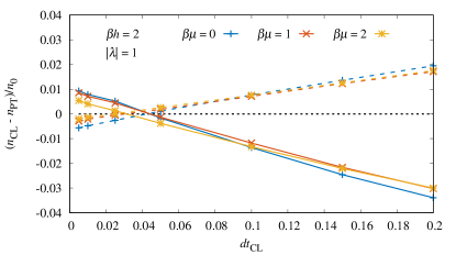
Figure 3: Density equation of state $n=n_{\uparrow}+n_{\downarrow}$ at $|\lambda|=1$ relative to the third-order perturbative result $n_{\text{PT}}$, normalized by the non-interacting, unpolarized counterpart $n_{0}$, as a function of the CL time step $dt_{\text{CL}}$, for three values of $\beta\mu$, all at $\beta h=2.0$. The dashed horizontal line shows the $n=n_{\text{PT}}$ line. The remaining differences at $dt_{\text{CL}}\to 0$ are likely a shortcoming of perturbation theory, but it would result in agreement between CL and the perturbative answers within the uncertainties shown in the other figures in this work, as in all cases the differences are reduced by a factor of 3 when $dt_{\text{CL}}\to 0$.

Generally speaking, our results speak favorably for the CL method as a way to tackle polarized matter, indicating that the door is open for calculations in higher dimensions and for non-trivial coupling strengths. More specifically, the results obtained with the various methods in the virial region are in remarkably good agreement with one another. For $\beta\mu\gtrsim-1.5$, small differences are noticeable in the density equation of state at strong coupling ($\lambda=2$), even less in the polarization.

It should be pointed out that fermions in 1D can be addressed without a sign problem by, e.g., mapping the system onto hard-core bosons (see e.g. Hirsch et al. (1982)) or employing the fermion bag approach Chandrasekharan (2013). However, to our acknowledge, such methods do not generalize (efficiently) to higher dimensions, which is why we focused here on benchmarks for auxiliary-field approaches. The latter not only generalize to higher dimensions but also to a wide range of situations including condensed matter, nuclear, and high-energy physics.

Acknowledgments.– We thank C. R. Shill for providing values of the interacting virial coefficients and L. Rammelmüller for useful discussions. This work was supported by HIC for FAIR within the LOEWE program of the State of Hesse and by the National Science Foundation under Grants No. DGE1144081 (Graduate Research Fellowship Program), PHY1452635 (Computational Physics Program).

Appendix A Results for higher interaction strengths: Density and polarization at $|\lambda|=2$.

Figure 4: Density equation of state $n=n_{\uparrow}+n_{\downarrow}$ normalized by the non-interacting, unpolarized counterpart $n_{0}$ for attractive (left) and repulsive (right) interactions of strength $\lambda=\pm 2$. Insets: Zoom in on the region $\beta\mu>0$ (left) and $\beta\mu>1$ (right). The CL results are shown with colored symbols, perturbative results at third order are shown with solid lines, and virial expansion results appear as dashed lines.

Figure 5: Spin polarization $m=n_{\uparrow}-n_{\downarrow}$ normalized by the non-interacting, unpolarized density $n_{0}$ for attractive (left) and repulsive (right) interactions of strength $\lambda=\pm 2$. The CL results are shown with colored symbols, perturbative results at third order are shown with solid lines, and virial expansion results appear as dashed lines.

In this Appendix we present the density and polarization equations of state analogous to Figs. 1 and 2, but for the stronger interaction strength of $|\lambda|=2$. The same techniques discussed for the results at $|\lambda|=1$ are applied here.

In Fig. 4 we show our results for the density equation of state at $\lambda=2$ (left) and $\lambda=-2$ (right), as a function of $\beta\mu$ and for varying asymmetry $\beta h=0,\dots,2.0$. We compare our CL results with third-order perturbation theory and the virial expansion for $\beta\mu\leq-1.5$. As expected, the agreement between all three techniques deteriorates at the increased coupling strength when compared to the results for $|\lambda|=1$. However, the overall comparison is satisfactory. For these systems, perturbation theory is expected to break down at this coupling strength. Indeed, this is most obvious for the unpolarized case which was further discussed in Ref. Loheac and Drut (2017). Agreement between perturbation theory and CL improves as the polarization increases, where the effective interaction between opposite spins lessens. The virial expansion demonstrates a more significant deterioration at this coupling as both $\beta\mu$ and $\beta h$ move away from $z_{s}\sim 0$.

In Fig. 5, we show our results for the polarization equation of state at $\lambda=2$ (left) and $\lambda=-2$ (right), as a function of $\beta\mu$ and for varying asymmetry $\beta h=0,\dots,2.0$. Also in this case we compare our CL results with perturbation theory calculations and find excellent agreement for the whole range of $\beta\mu$ studied.

Appendix B Perturbative progression from first to third order.

Figure 6: Density $n=n_{\uparrow}+n_{\downarrow}$ normalized by the non-interacting, unpolarized counterpart $n_{0}$ for attractive interaction of strength $\lambda=1$ (left) and $\lambda=2$ (right). The CL results are shown with black diamonds, perturbative results at first (NLO), second (N2LO), and third (N3LO) order are shown with dotted, dashed, and solid lines, respectively.

Finally, in Fig. 6 we show the progression of density results in lattice perturbation theory at first, second, and third order, for two attractive couplings ($\lambda=1,2$) and for two polarizations ($\beta h=1.0,2.0$). We note that the perturbative results appear very well converged at $\lambda=1$, where they agree very well with the CL answers, as noted in the main text. On the other hand, at $\lambda=2$, perturbation theory is (as expected) still slightly away from convergence [note in particular the big jump from first (dotted) to second order (dashed)], but it uniformly approaches the CL results.

References

- Casalbuoni and Nardulli (2004) R. Casalbuoni and G. Nardulli, Rev. Mod. Phys. 76, 263 (2004), hep-ph/0305069 .
- Radzihovsky and Sheehy (2010) L. Radzihovsky and D. E. Sheehy, Rep. Prog. Phys. 73, 076501 (2010), arXiv:0911.1740 [cond-mat.quant-gas] .
- Chevy and Mora (2010) F. Chevy and C. Mora, Rep. Prog. Phys. 73, 112401 (2010), arXiv:1003.0801 [cond-mat.quant-gas] .
- Gubbels and Stoof (2013) K. Gubbels and H. Stoof, Phys. Rep. 525, 255 (2013).
- Porter and Drut (2017) W. J. Porter and J. E. Drut, Phys. Rev. A 95, 053619 (2017), arXiv:1609.09401 [cond-mat.quant-gas] .
- Rammelmüller et al. (2017a) L. Rammelmüller, J. E. Drut, and J. Braun, in 19th International Conference on Recent Progress in Many-Body Theories (RPMBT19) Pohang, Korea, June 25-30, 2017 (2017) arXiv:1710.11421 [cond-mat.quant-gas] .
- Drut (2017) J. E. Drut, in 19th International Conference on Recent Progress in Many-Body Theories (RPMBT19) Pohang, Korea, June 25-30, 2017 (2017) arXiv:1710.10176 [cond-mat.quant-gas] .
- Loheac et al. (2018) A. C. Loheac, J. Braun, and J. E. Drut, Proceedings, 35th International Symposium on Lattice Field Theory (Lattice 2017): Granada, Spain, June 18-24, 2017, EPJ Web Conf. 175, 03007 (2018), arXiv:1710.05020 [cond-mat.quant-gas] .
- Shill and Drut (2018) C. R. Shill and J. E. Drut, Proceedings, 35th International Symposium on Lattice Field Theory (Lattice 2017): Granada, Spain, June 18-24, 2017, EPJ Web Conf. 175, 03003 (2018), arXiv:1710.03247 [hep-lat] .
- Loheac and Drut (2017) A. C. Loheac and J. E. Drut, Phys. Rev. D 95, 094502 (2017), arXiv:1702.04666 [hep-lat] .
- Takahashi (2004) M. Takahashi, ed., Quantum Physics in One Dimension (Oxford University Press, Oxford, 2004).
- Giamarchi (1999) T. Giamarchi, ed., Thermodynamics of One-Dimensional Solvable Models (Cambridge University Press, Cambridge, 1999).
- Guan et al. (2013) X.-W. Guan, M. T. Batchelor, and C. Lee, Rev. Mod. Phys. 85, 1633 (2013).
- Loheac et al. (2015) A. C. Loheac, J. Braun, J. E. Drut, and D. Roscher, Phys. Rev. A 92, 063609 (2015), arXiv:1508.03314 [cond-mat.quant-gas] .
- Braun et al. (2013) J. Braun, J.-W. Chen, J. Deng, J. E. Drut, B. Friman, C.-T. Ma, and Y.-D. Tsai, Phys. Rev. Lett. 110, 130404 (2013), arXiv:1209.3319 [cond-mat.stat-mech] .
- Braun et al. (2015) J. Braun, J. E. Drut, and D. Roscher, Phys. Rev. Lett. 114, 050404 (2015), arXiv:1407.2924 [cond-mat.quant-gas] .
- Rammelmüller et al. (2017b) L. Rammelmüller, W. J. Porter, J. E. Drut, and J. Braun, Phys. Rev. D 96, 094506 (2017b), arXiv:1708.03149 [cond-mat.quant-gas] .
- Roscher et al. (2014a) D. Roscher, J. Braun, J.-W. Chen, and J. E. Drut, J. Phys. G 41, 055110 (2014a), arXiv:1306.0798 [cond-mat.stat-mech] .
- Roscher et al. (2014b) D. Roscher, J. Braun, and J. E. Drut, Phys. Rev. A 89, 063609 (2014b), arXiv:1311.0179 [cond-mat.quant-gas] .
- Roscher et al. (2015) D. Roscher, J. Braun, and J. E. Drut, Phys. Rev. A 91, 053611 (2015), arXiv:1501.05544 [cond-mat.quant-gas] .
- Wang et al. (2017) J. Wang, Y. Che, L. Zhang, and Q. Chen, ArXiv e-prints (2017), arXiv:1703.00161 [cond-mat.supr-con] .
- Frank et al. (2018) B. Frank, J. Lang, and W. Zwerger, ArXiv e-prints (2018), arXiv:1804.03035 [cond-mat.quant-gas] .
- Lee (2009) D. Lee, Prog. Part. Nucl. Phys. 63, 117 (2009), arXiv:0804.3501 [nucl-th] .
- Drut and Nicholson (2013) J. E. Drut and A. N. Nicholson, J. Phys. G 40, 043101 (2013), arXiv:1208.6556 [cond-mat.stat-mech] .
- Aarts et al. (2010) G. Aarts, E. Seiler, and I.-O. Stamatescu, Phys. Rev. D 81, 054508 (2010), arXiv:0912.3360 [hep-lat] .
- Aarts et al. (2011) G. Aarts, F. A. James, E. Seiler, and I.-O. Stamatescu, Eur. Phys. J. C 71, 1756 (2011), arXiv:1101.3270 [hep-lat] .
- Aarts et al. (2017) G. Aarts, E. Seiler, D. Sexty, and I.-O. Stamatescu, JHEP 05, 044 (2017), [Erratum: JHEP01,128(2018)], arXiv:1701.02322 [hep-lat] .
- Nagata et al. (2016) K. Nagata, J. Nishimura, and S. Shimasaki, Phys. Rev. D 94, 114515 (2016), arXiv:1606.07627 [hep-lat] .
- Bloch et al. (2017) J. Bloch, J. Meisinger, and S. Schmalzbauer, Proceedings, 34th International Symposium on Lattice Field Theory (Lattice 2016): Southampton, UK, July 24-30, 2016, PoS LATTICE2016, 046 (2017), arXiv:1701.01298 [hep-lat] .
- Bloch (2017) J. Bloch, Phys. Rev. D 95, 054509 (2017), arXiv:1701.00986 [hep-lat] .
- Attanasio and Jäger (2016) F. Attanasio and B. Jäger, Proceedings, 34th International Symposium on Lattice Field Theory (Lattice 2016): Southampton, UK, July 24-30, 2016, PoS LATTICE2016, 053 (2016), arXiv:1610.09298 [hep-lat] .
- Aarts et al. (2016) G. Aarts, F. Attanasio, B. Jäger, and D. Sexty, Proceedings, International Meeting Excited QCD 2016: Costa da Caparica, Portugal, March 6-12, 2016, Acta Phys. Polon. Supp. 9, 621 (2016), arXiv:1607.05642 [hep-lat] .
- Shill and Drut (tion) C. R. Shill and J. E. Drut, (in preparation).
- Rammelmüller et al. (2017c) L. Rammelmüller, W. J. Porter, J. Braun, and J. Drut, Phys. Rev. A 96, 033635 (2017c), arXiv:1706.00031 [cond-mat.quant-gas] .
- Endres et al. (2011) M. G. Endres, D. B. Kaplan, J.-W. Lee, and A. N. Nicholson, Phys. Rev. Lett. 107, 201601 (2011).
- DeGrand (2012) T. DeGrand, Phys. Rev. D 86, 014512 (2012).
- Drut and Porter (2015) J. E. Drut and W. J. Porter, Phys. Rev. B 92, 125126 (2015).
- Drut and Porter (2016) J. E. Drut and W. J. Porter, Phys. Rev. E 93, 043301 (2016).
- Shi and Zhang (2016) H. Shi and S. Zhang, Phys. Rev. E 93, 033303 (2016).
- Hirsch et al. (1982) J. E. Hirsch, R. L. Sugar, D. J. Scalapino, and R. Blankenbecler, Phys. Rev. B 26, 5033 (1982).
- Chandrasekharan (2013) S. Chandrasekharan, Eur. Phys. J. A 49, 90 (2013), arXiv:1304.4900 [hep-lat] .