Topological Data Analysis for Object Data

Abstract

Statistical analysis on object data presents many challenges. Basic summaries such as means and variances are difficult to compute. We apply ideas from topology to study object data. We present a framework for using persistence landscapes to vectorize object data and perform statistical analysis. We apply to this pipeline to some biological images that were previously shown to be challenging to study using shape theory. Surprisingly, the most persistent features are shown to be “topological noise” and the statistical analysis depends on the less persistent features which we refer to as the “geometric signal”. We also describe the first steps to a new approach to using topology for object data analysis, which applies topology to distributions on object spaces.

Keywords: topological data analysis; persistence landscapes; object spaces; extrinsic object data analysis; .

1 Introduction

Object data may be considered to be sampled from some underlying object space, which may be a manifold or stratified space. Topology produces homology invariants that lend themselves to the investigation of holes or voids in this underlying structure. Topological data analysis (TDA) uses distance (i.e. metric) data to provide a multiscale summary of these topological features.

In the remainder of the introduction, we summarize: our framework for using topological data analysis for object data; our results; and make comparisons to related work. Mathematical terms that will be define in Sections 2 and 4 are in italics, and non-technical terms that are explained in Section 3 are in double quotes.

1.1 TDA framework for object data

The methods of topological data analysis are quite flexible, and there are many possible ways to apply them to object data. We will use persistent homology. The crucial step is encoding the object data by an increasing sequence of spaces that contain enough of the structure so that the subsequent statistical analysis will be successful. We will represent the object data by a finite sample of points. From the pairwise distances between these points we will construct an increasing family of simplicial complexes, called Vietoris-Rips complexes. We will calculate their persistent homology and convert this data to vectors using death vectors and persistence landscapes. These vectors will constitute our topological summary of the object data and we will the input to our statistical analysis.

1.2 Results

We applied the pipeline described above to a collection of images of leaves (see Figure 4). Looking at these images, we see a number of regions bounded by the veins, the midrib (the large central vein), and the boundary of the leaf. These regions are approximately rectangular shaped and their boundaries are topologically equivalent (homeomorphic or homotopy equivalent) to circles. Furthermore, the union of these boundaries (the veins and the boundary of the leaf) is topologically equivalent (has the same homotopy-type as) a collection of circles attached at a common point (a wedge or bouquet of circles). We expected that our analysis would be insensitive to “geometric noise” and detect this “topological signal” (homotopy-type).

In fact, the analysis was successful for the opposite reason. The point samples we obtained from the leaves were of low quality (see Figure 8). From these points it was impossible to see all of the rectangular regions of the leaves, and in addition, outlier points (see the bottom of Figure 8) created “topological noise”. However, the arrangement of sampled points contained enough geometric information on the leaves so that our statistical analysis was successful by using this “geometric signal”.

1.3 Related work

Our approach and results are closely related to work by Bendich et al. (2016) [2], who also applied TDA to object data. In their case they considered brain artery structures extracted from magnetic resonance images and applied persistence homology, which was encoded in vectors by the order statistic on the most persistent points in the persistence diagram. Also, closely related is work by Kovacev-Nikolic et al. (2016) [32] who applied persistent homology and persistence landscapes to protein structure data.

Our analysis differs by considering lower quality data (see Figure 8), using a sophisticated feature vector (the persistence landscape from which the persistence diagram can be reconstructed), and in highlighting the distinction between “topological noise” and “geometric signal”.

Outline of the paper

In Section 2 we summarize parts of topological data analysis (TDA) and introduce our framework for applying TDA to object data. In Section 3 we apply our framework to a particular set of object data. In Section 4 we introduce a new approach that applies differential or algebraic topology methods to data analysis of distributions on object spaces.

2 Objects TDA

Topological data analysis (TDA) summarizes the topological and geometric structure of data by applying tools from algebraic topology to certain geometric structures built from the data at hand.

2.1 Simplicial complexes

The basic building block is a simplex, which we will now define. A $0$-simplex is a single point or vertex, a $1$-simplex is the line segment or edge determined by $2$ distinct vertices, $2$-simplex is the solid triangle determined by $3$ vertices, that do not lie on a line, and so on. More formally, a $p$-simplex is the convex hull of points $x_{0},x_{1},\ldots,x_{p}\in\mathbb{R}^{d}$ such that the vectors $x_{1}-x_{0},\ldots,x_{p}-x_{0}$ are linearly independent.

In data-analytic applications, one treats a data point cloud, $\mathcal{X}$, as a noisy sampling of a metric space $\mathcal{M}$. In topological data analysis, one obtains summaries of the topology and geometry of $\mathcal{M}$ by defining a parametric family of nested simplicial complexes which is built on top of $\mathcal{X}$ and considering its topology. This family is known as a filtered simplicial complex or simply a filtration.

There are a number of different complexes which are used in topological data analysis. For example, we may consider a coarse-graining of $\mathcal{X}$ by taking the union of closed $\varepsilon$-neighborhoods;

$$\mathcal{X}_{\varepsilon}=\bigcup_{x\in\mathcal{X}}B_{\varepsilon}(x),\text{ where }B_{\varepsilon}(x)\left\{y\in\mathcal{M}:d\left(x,y\right)\leq\varepsilon\right\}.$$

The Čech complex is mainly of theoretical interest and is defined as follows.

Definition 1.

The Čech complex, $\mathcal{C}_{\varepsilon}$, generated from $\mathcal{X}$ is the simplicial complex which has a $p$-simplex whenever the closed $\varepsilon$-neighborhoods of subset of $p$ data cloud points have a common intersection (this is also called the nerve of cover $\mathcal{X}_{\varepsilon}$).

Figure 1 shows for a certain finite set of points $\mathcal{X}$ in the plane, the disks composing $\mathcal{X}_{\varepsilon}$ and the corresponding Čech complexes, $\mathcal{C}_{\varepsilon}$, for disks of radii $\varepsilon=0.053,0.184,0.316$ and $0.5$.

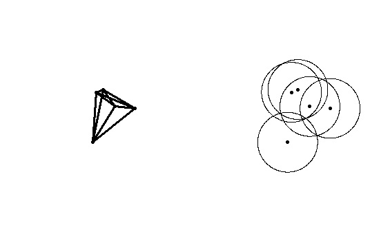
Figure 1: Čech complexes of a point cloud for various radii.

The Nerve theorem states that if $\mathcal{M}=\mathbb{R}^{d}$ then the homotopy types of $\mathcal{C}_{\varepsilon}$ and $\mathcal{X}_{\varepsilon}$ are the same. This means that Čech complex, $\mathcal{C}_{\varepsilon}$, is a topologically faithful simplicial model for the topology of $\mathcal{X}_{\varepsilon}$, a point cloud fattened by balls. Unfortunately, it is often expensive to compute and to store the Čech complex since to determine the $p$-simplices one has to compute all subsets of size $p$ of which there are a total of $2^{p}$. The Vietoris-Rips complex, which we now define, is a more computationally efficient alternative to the Čech complex.

Definition 2.

The Vietoris-Rips (VR) complex, $\mathcal{R}_{\varepsilon}$, generated from open cover $\mathcal{X}_{\varepsilon}$ is the simplicial complex which has a $p$-simplex any time that the closed $\varepsilon$-neighborhoods for subset of $p$ points all have pairwise nonempty intersections.

All Vietoris-Rips complexes $\mathcal{R}_{\varepsilon}$ (for all $\varepsilon$) can be computed for $n$ data cloud points once one has computed all $\binom{n}{2}$ pairwise distances.

In general, there is no single proximity parameter $\varepsilon$ that yields a Vietoris-Rips complex $\mathcal{R}_{\varepsilon}$ which best describes the topological and geometric structure from which that data point cloud was sampled. Instead one considers all possible values of $\varepsilon$ and one determines which topological features persist as $\varepsilon$ increases.

2.2 Persistent homology

Persistent homology completely describes how homology persists as one steps through the filtration. For example, consider a filtration of Vietoris-Rips complexes

$$\mathcal{R}_{\varepsilon_{0}}\subset\mathcal{R}_{\varepsilon_{1}}\subset\cdots\subset\mathcal{R}_{\varepsilon_{m}},$$

for $\varepsilon_{0}<\varepsilon_{1}<\cdots<\varepsilon_{m}$. One is interested in topological features that persist as the proximity parameter $\varepsilon$ ranges from $\varepsilon_{0}$ to $\varepsilon_{m}$. For a given value of $\varepsilon$, the number of $p$-dimensional holes of the Vietoris-Rips complex $\mathcal{R}_{\varepsilon}$ is determined as the dimension of the vector space given by the $p$th homology group $H_{p}(\mathcal{R}_{\varepsilon})$, where coefficients are taken to be in some fixed field, typically $\mathbb{Z}/2$. Let

$$\beta_{p}\left(\mathcal{R}_{\varepsilon}\right)=\dim\left[H_{p}\left(\mathcal{R}_{\varepsilon}\right)\right]$$

which is known as the $p$th Betti number. For instance, $\beta_{0}\left(\mathcal{R}_{\varepsilon}\right)$ is the number of connected components or clusters of the point cloud data set while $\beta_{1}\left(\mathcal{R}_{\varepsilon}\right)$ the number of holes or tunnels in the Vietoris-Rips complex $\mathcal{R}_{\varepsilon}$. However, even knowing the Betti numbers at all values of $\varepsilon$, one has no information on whether or not the corresponding topological features persist from one value of $\varepsilon$ to the next. Persistent homology remedies this defect by encoding not only the Betti numbers, but the persistent Betti numbers, given by

$$\beta_{i}^{j}=\operatorname{rank}\left(H_{p}(\mathcal{R}_{\varepsilon_{i}})\to H_{p}(\mathcal{R}_{\varepsilon_{j}})\right)$$

where $H_{p}(\mathcal{R}_{\varepsilon_{i}})\to H_{p}(\mathcal{R}_{\varepsilon_{j}})$ is the linear map induced by the inclusions $\mathcal{R}_{\varepsilon_{i}}\subset\mathcal{R}_{\varepsilon_{j}}$. The image of this linear map is called a persistent homology group.

The persistence diagram gives a complete summary of persistent homology as a collection of points $\{(b,d)\}$, where each $(\varepsilon_{i},\varepsilon_{j})$ represents a homology class that is born at $\varepsilon_{i}$ and dies at $\varepsilon_{j}$. To be precise, the multiplicity of the point $(\varepsilon_{i},\varepsilon_{j})$ in the persistence diagram is given by

$$\mu_{i}^{j}=\beta_{i-1}^{j}-\beta_{i}^{j}+\beta_{i}^{j-1}-\beta_{i-1}^{j-1}.$$

See [13] for more details. Two persistence diagrams are given in Figure 2. For a point $(b,d)$ in the persistence diagram, the quantity $d-b$ is called its persistence.

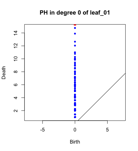
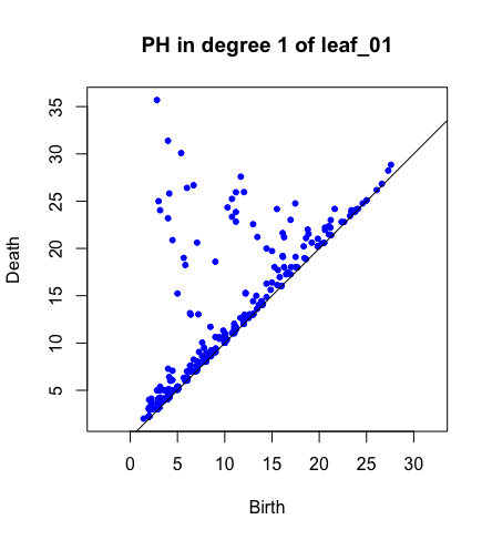
Figure 2: Persistence diagrams for homology in degree 0 (left) and degree 1 (right) of a Vietoris-Rips complex.

It is sometimes said that proximity parameter $\varepsilon$ ranges from $\varepsilon_{0}$ to $\varepsilon_{m}$ short-lived topological features are assumed to represent topological (statistical) noise while the features which persist over a wide range proximity parameter $\varepsilon$ values represent a topological signal. However, we will show that it can be the case that long-lived features represent noise and that short-lived features represent a geometric signal.

Remark 3.

Persistent homology of the Čech complex and the Vietoris-Rips complex. Note that while, in general, the homotopy types of $\mathcal{R}_{\varepsilon}$ and $\mathcal{X}_{\varepsilon}$ are not the same, it is true that for all $\varepsilon$

$$\mathcal{C}_{\varepsilon}\subset\mathcal{R}_{\varepsilon}\subset\mathcal{C}_{2\varepsilon}$$

Which means that if Čech complexes $\mathcal{C}_{\varepsilon}$ and $\mathcal{C}_{2\varepsilon}$ are effective in detecting persistent topological and geometric features then $\mathcal{R}_{\varepsilon}$ will also be effective.

2.3 Persistence landscapes and statistical inference

In order to facilitate statistical inference we wish to give a complete (i.e. invertible) unique (i.e. injective) encoding of the persistence diagram as a vector.

For the Vietoris-Rips complex, since all vertices appear at filtration value $0$, all of the points in the persistence diagram for homology in degree 0 have birth coordinate 0 (see the left side of Figure 2). Thus, all of the information is included in the death times (the times when connected components merge). As such, we encode the persistence diagram using the corresponding order statistic. We call this the death vector. See the left hand side of Figure 3.

For more general persistence diagrams, such as for homology in degree 1 for the Vietoris-Rips complex (see the right hand figure in Figure 2), we use the persistence landscape [7], which we now describe.

For each point $(b,d)$ in the persistence diagram, consider the following function

$$f_{(b,d)}(t)=\begin{cases}t-b,\quad\text{if }b\leq t<\frac{b+d}{2},\\ d-t,\quad\text{if }\frac{b+d}{2}\leq t<d,\\ 0,\quad\text{otherwise}.\end{cases}$$

Then for $k\geq 1$, the $k$th persistence landscape function of the persistence diagram $\mathcal{D}$ is given by

$$\lambda_{k}(t)=\operatorname{kmax}_{(b_{i},d_{i})\in\mathcal{D}}f_{(b_{i},d_{i})}(t),$$

where $\operatorname{kmax}$ denotes the $k$th largest element. The persistence landscape consists of the sequence of functions $\{\lambda_{1},\lambda_{2},\lambda_{3},\ldots\}$. Notice that by definition, for all $t\in\mathbb{R}$, $\lambda_{1}(t)\geq\lambda_{2}(t)\geq\lambda_{3}(t)\geq\ldots$. That is, the persistence landscape is a decreasing sequence of functions.

It remains to turn this sequence of functions into a vector. This is done be evaluating the functions on a grid. Specifically, we evaluate the persistence landscape functions $\lambda_{1},\ldots,\lambda_{K}$ for some sufficiently large $K$ at the values $a,a+\delta,a+2\delta,a+3\delta,\ldots,a+m\delta$ for appropriate choices of $a$, $\delta$ and $m$. The resulting values are concatenated to obtain a vector in $\mathbb{R}^{K(m+1)}$.

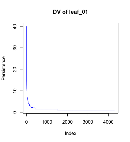
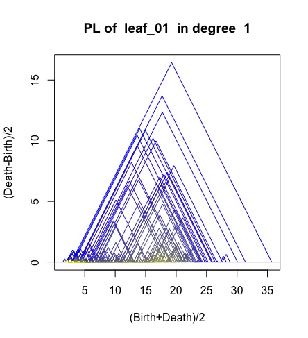
Figure 3: The death vector and persistence landscape corresponding to the persistence diagrams in Figure 2.

3 Objects TDA Example

Here we analyze the leaf data from Patrangenaru et al. (2016) [43] (see www.stat.fsu.edu/$\sim$vic/Original-figures). This image data set consists of two leaves, call them leaf A and leaf B, from the same tree. Twenty pictures were taken of each leaf from different perspectives, to yield a total of 40 pictures which are shown below in Figure 5. Two larger images are shown in Figure 4.

Figure 4: Sample original images of leaf A (left) and leaf B (right).

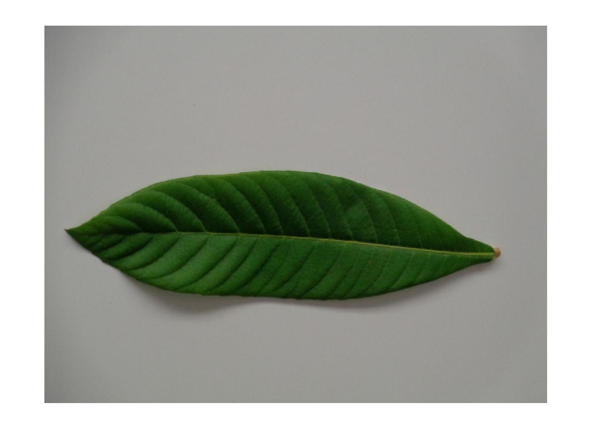
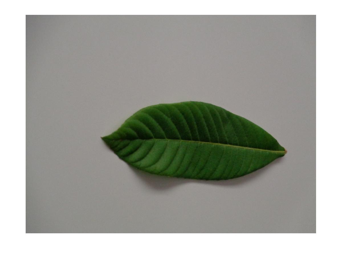
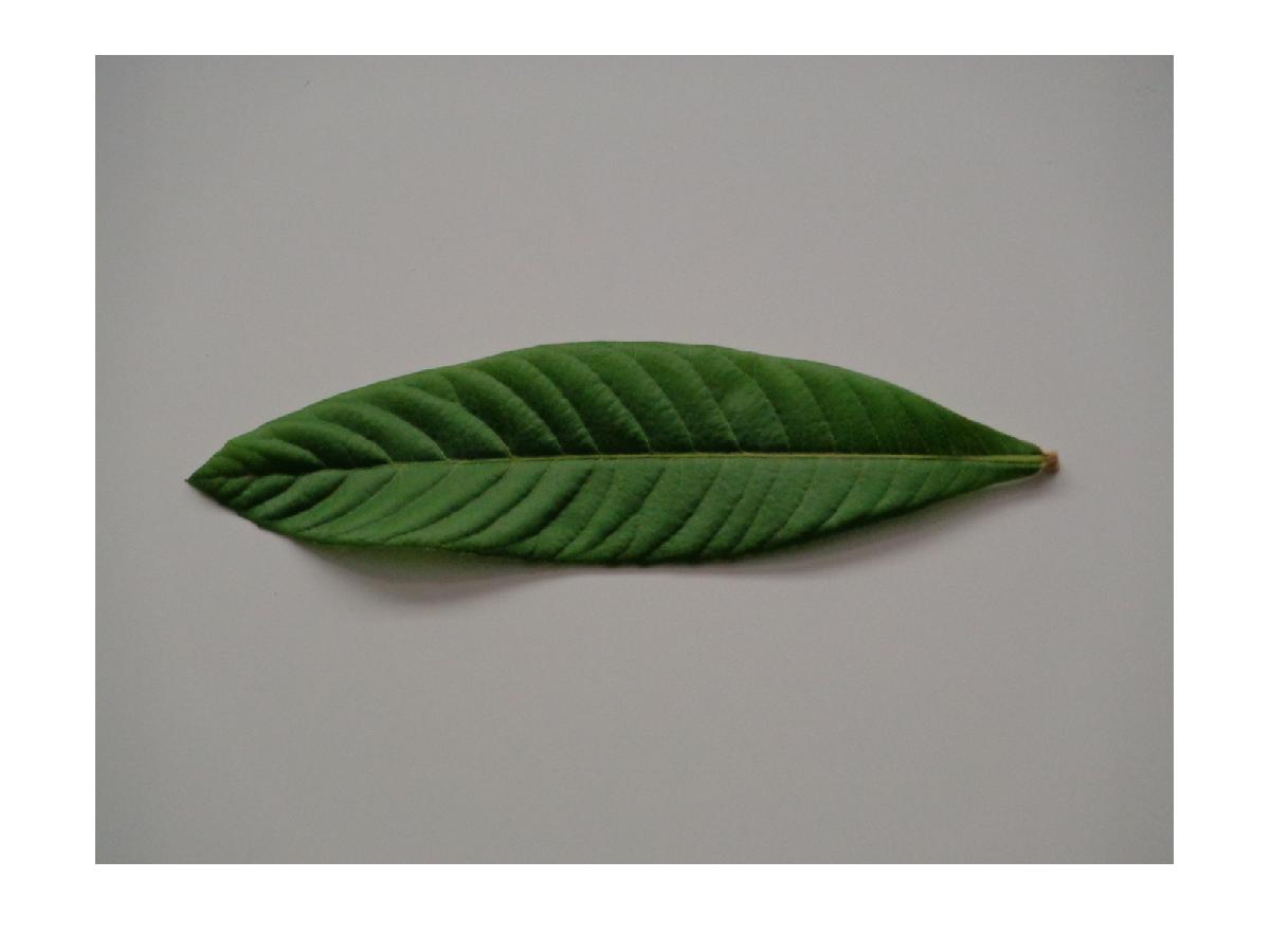
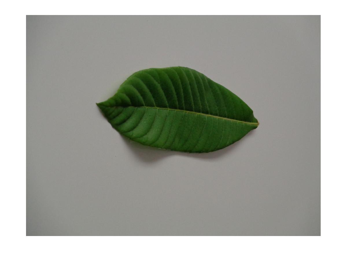
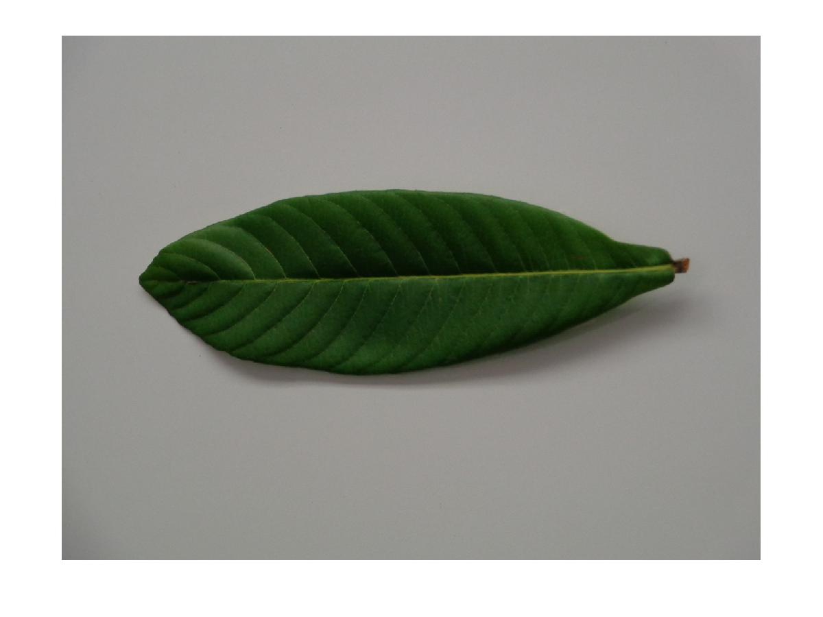
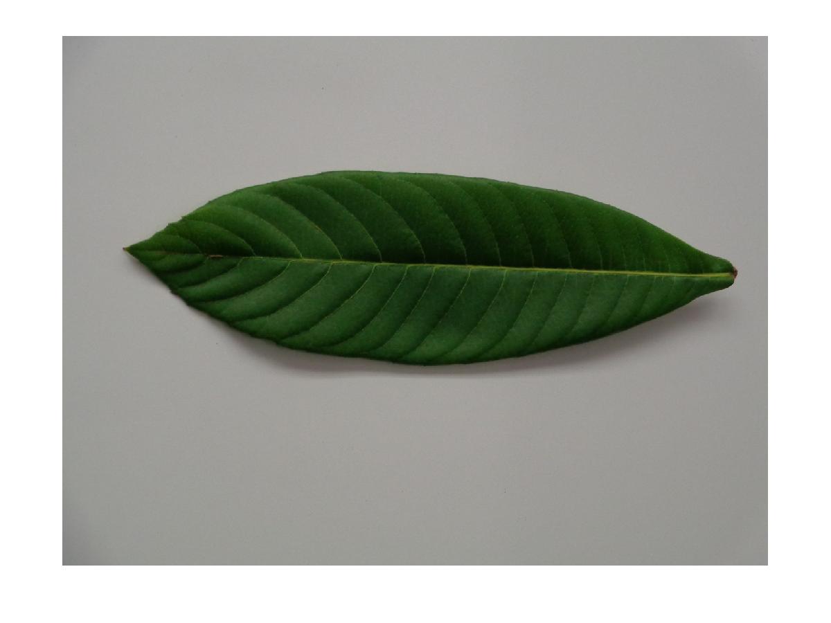
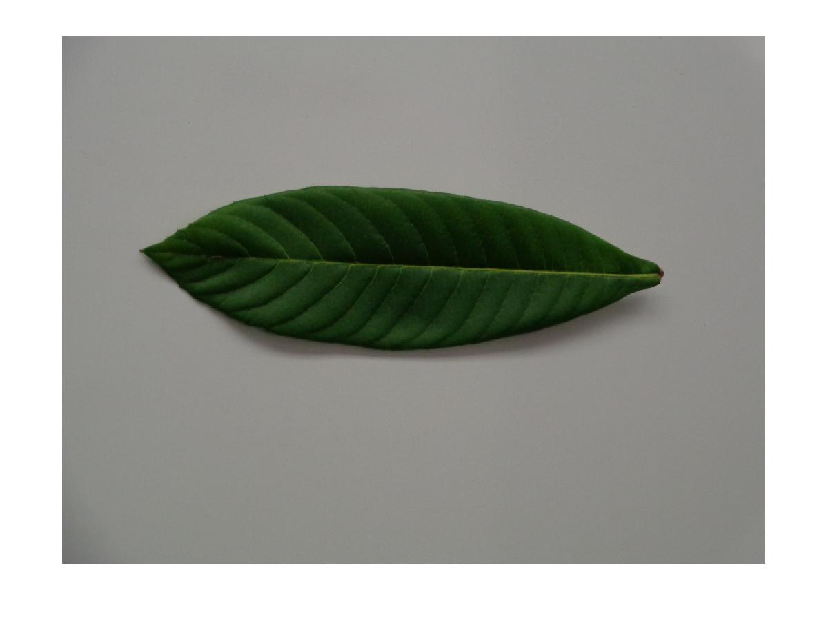
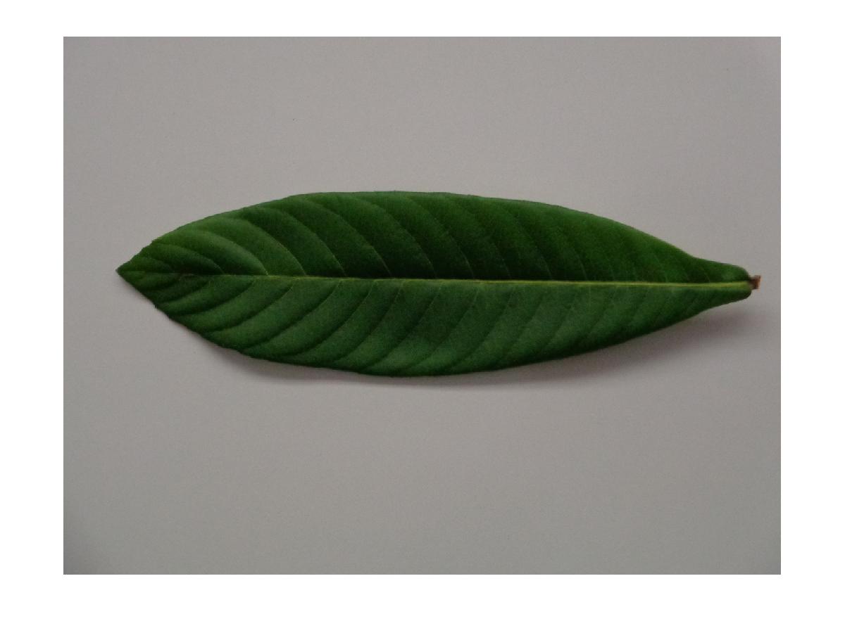
Figure 5: Original images of leaf A (top 20 figures) and leaf B (bottom 20 figures).

Next a contour each of the 40 pictures was extracted, in MATLAB with using an edge map, and then pairs of 2-dimensional contours were matched in resulting in ten matched pairs of contours for each leaf using the method of Ellingson et al. (2013)[21]. After this a 3-dimensional contour was reconstructed using the classical eight point algorithm (see for instance Ma et al. (2006)[33]) from each pair of 2-dimensional contours to yield a total of ten reconstructed 3-dimensional contour for each leaf. The two samples of 3-dimensional (reconstructed) contours for leaves A (left) and B (right) as shown in Figure 6.

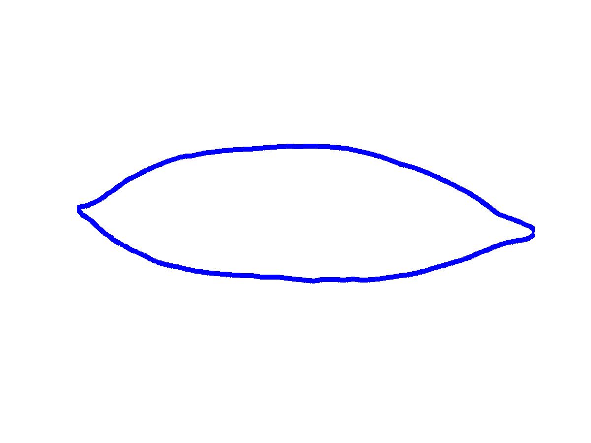
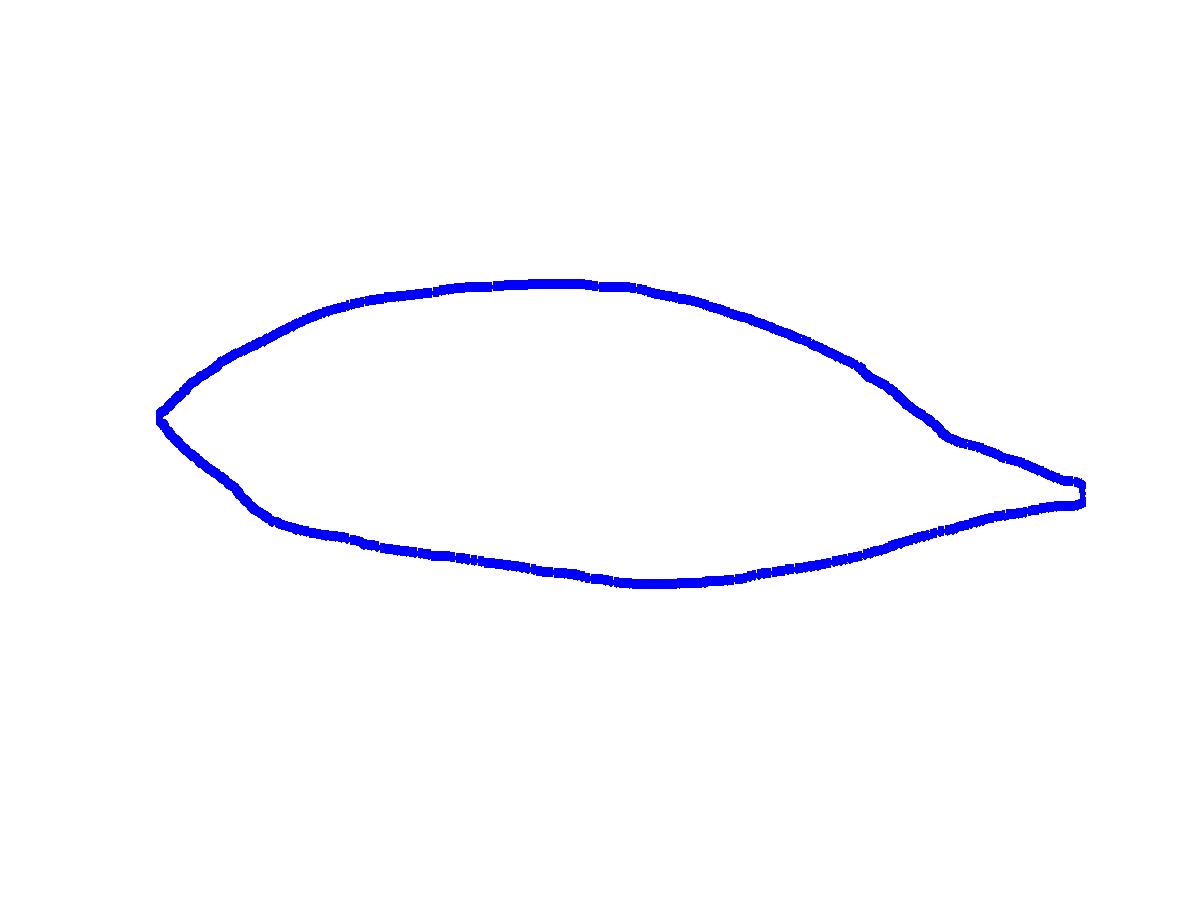
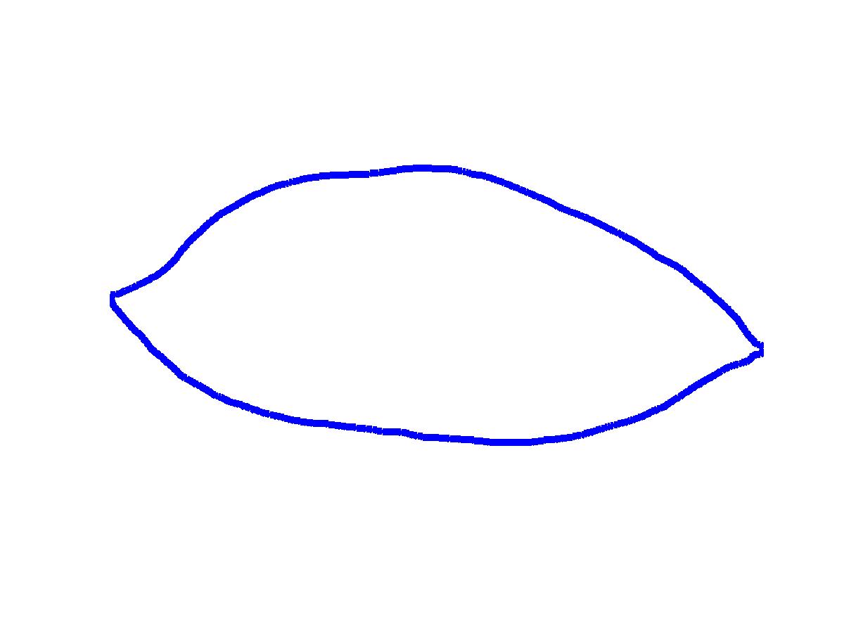
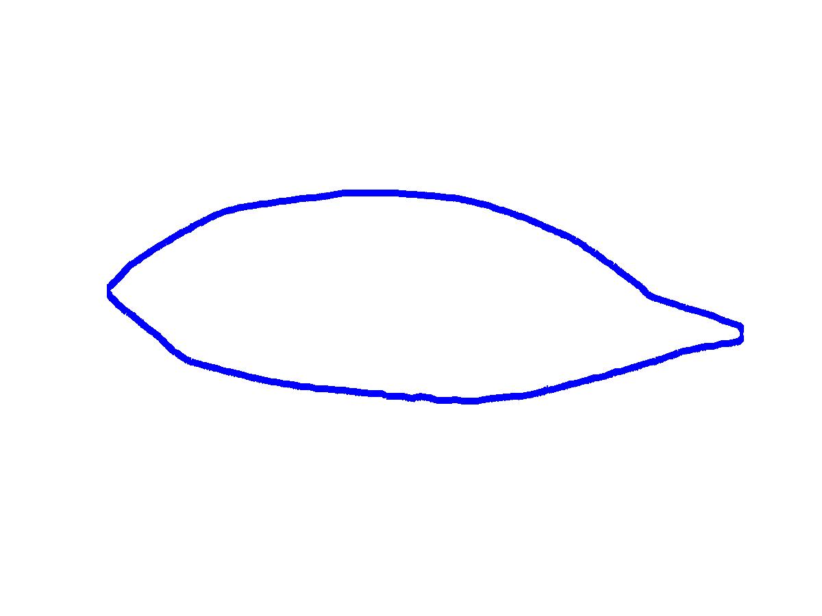
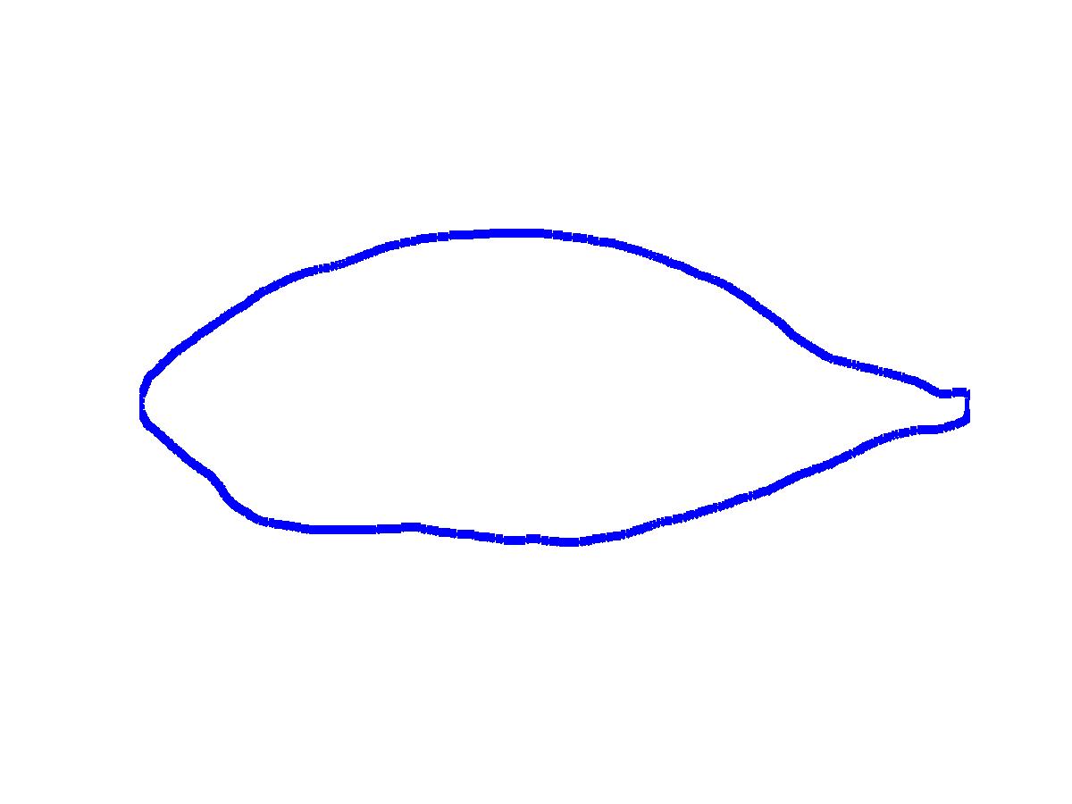
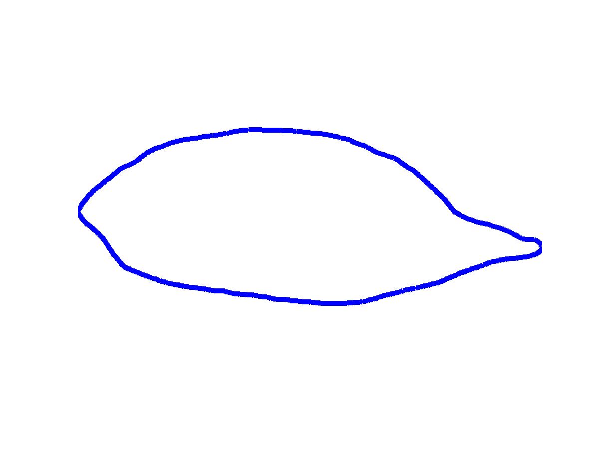
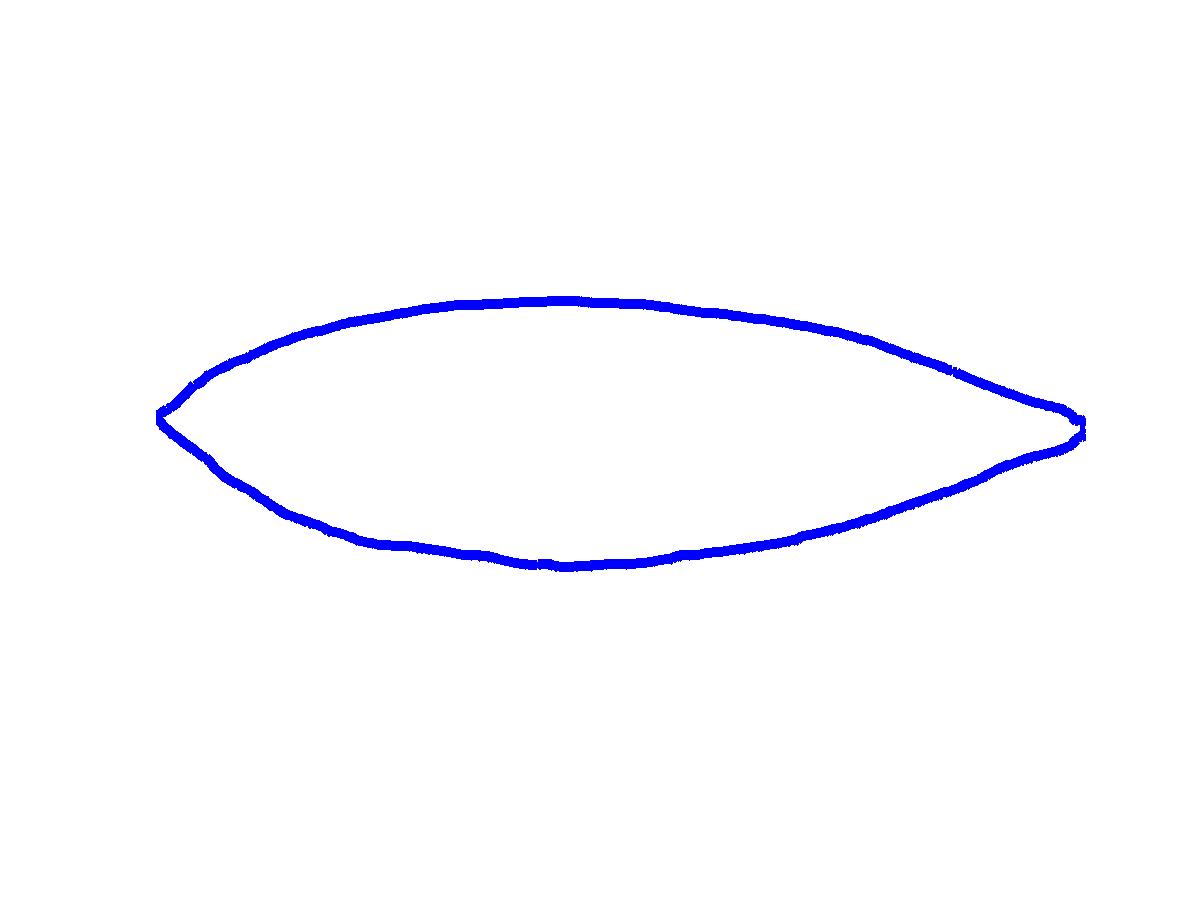
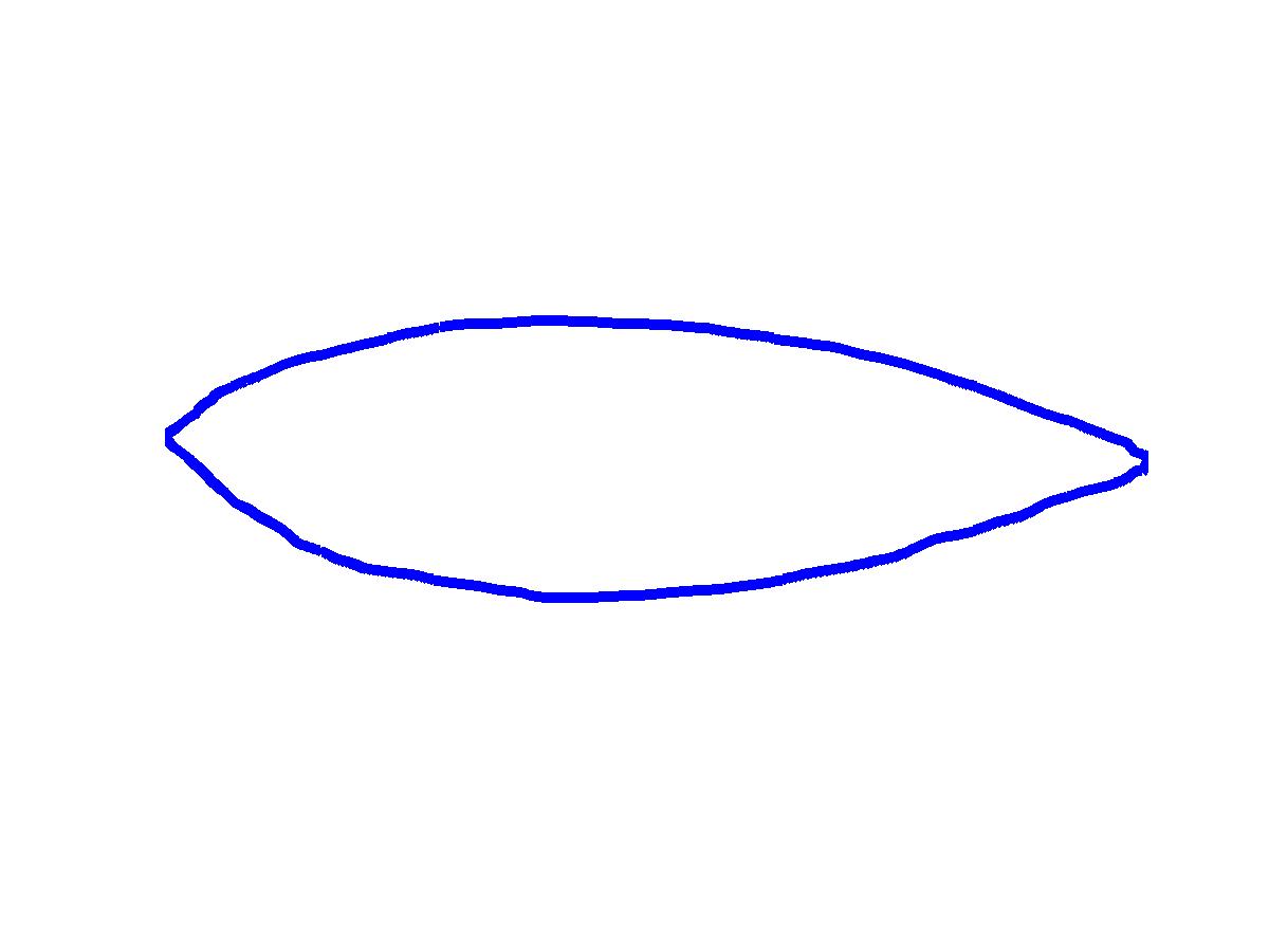
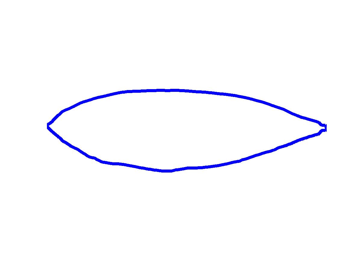
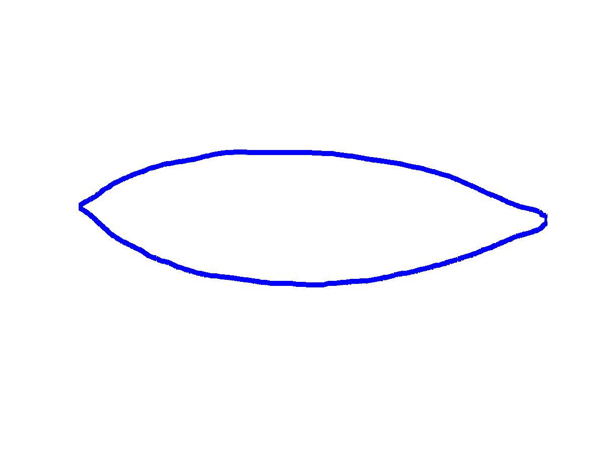
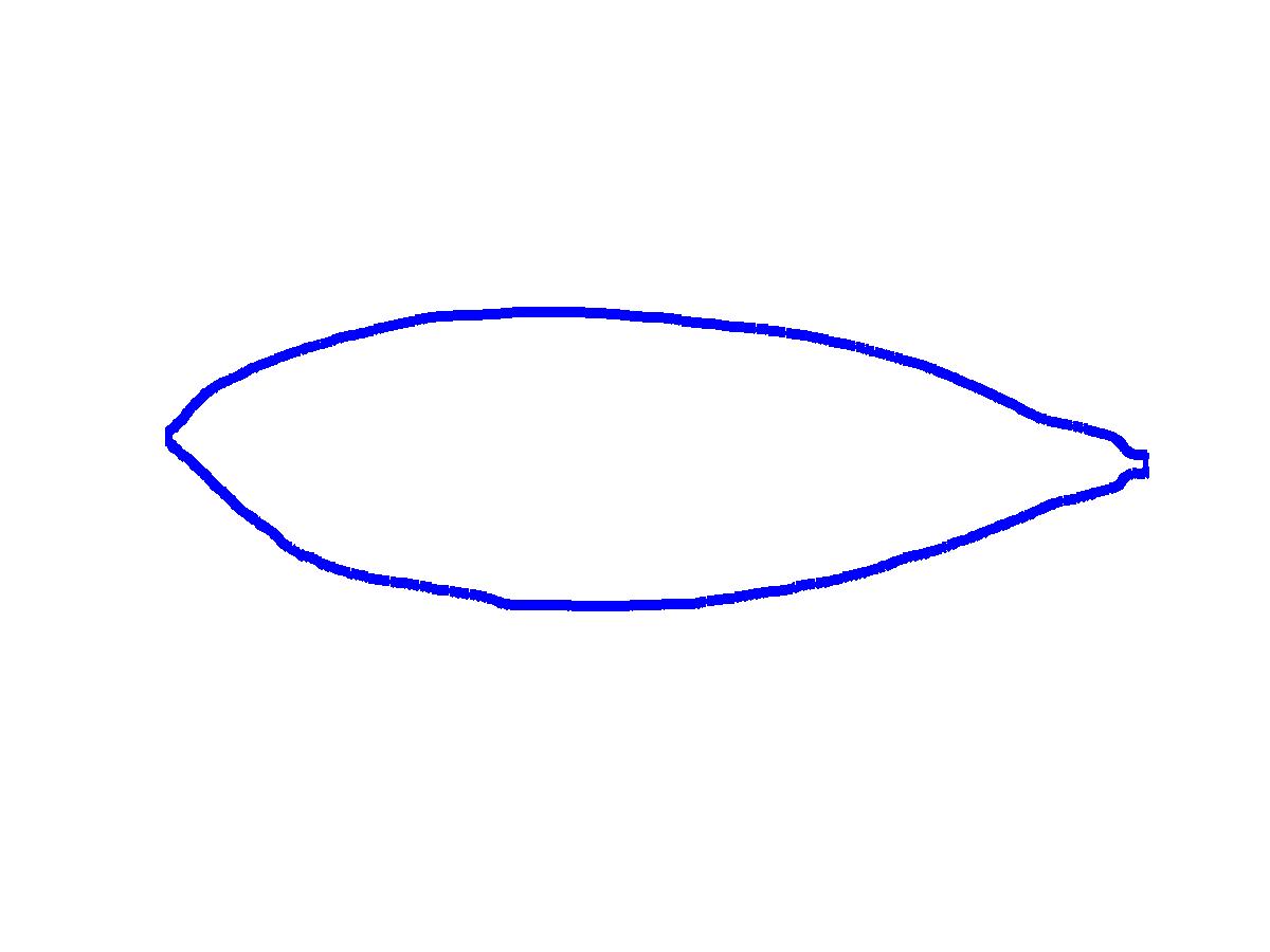
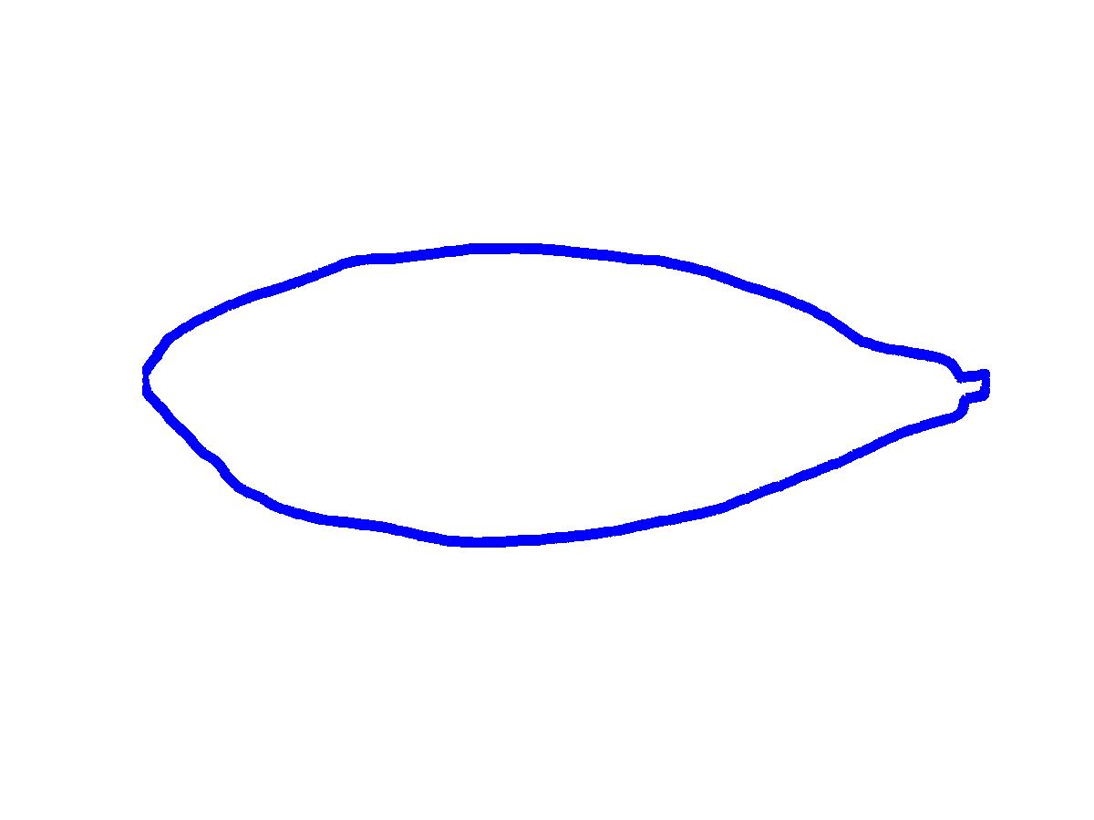
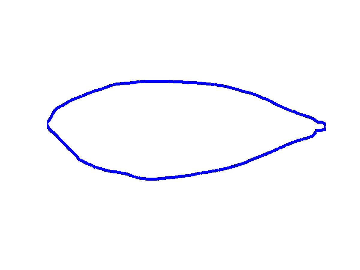
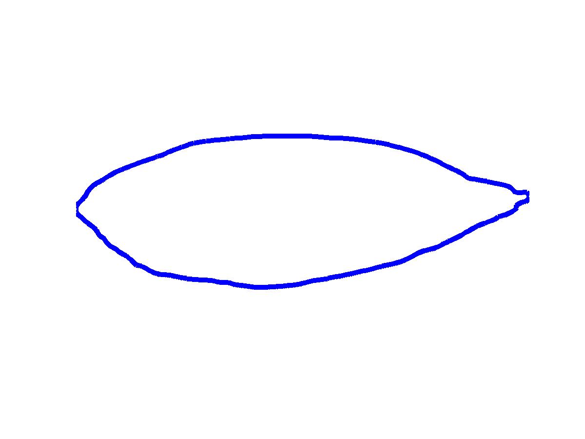
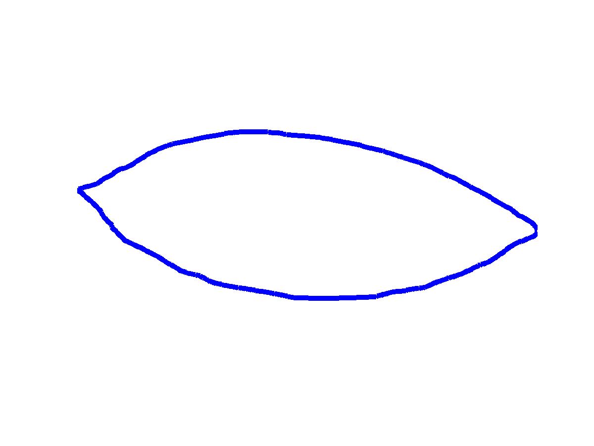
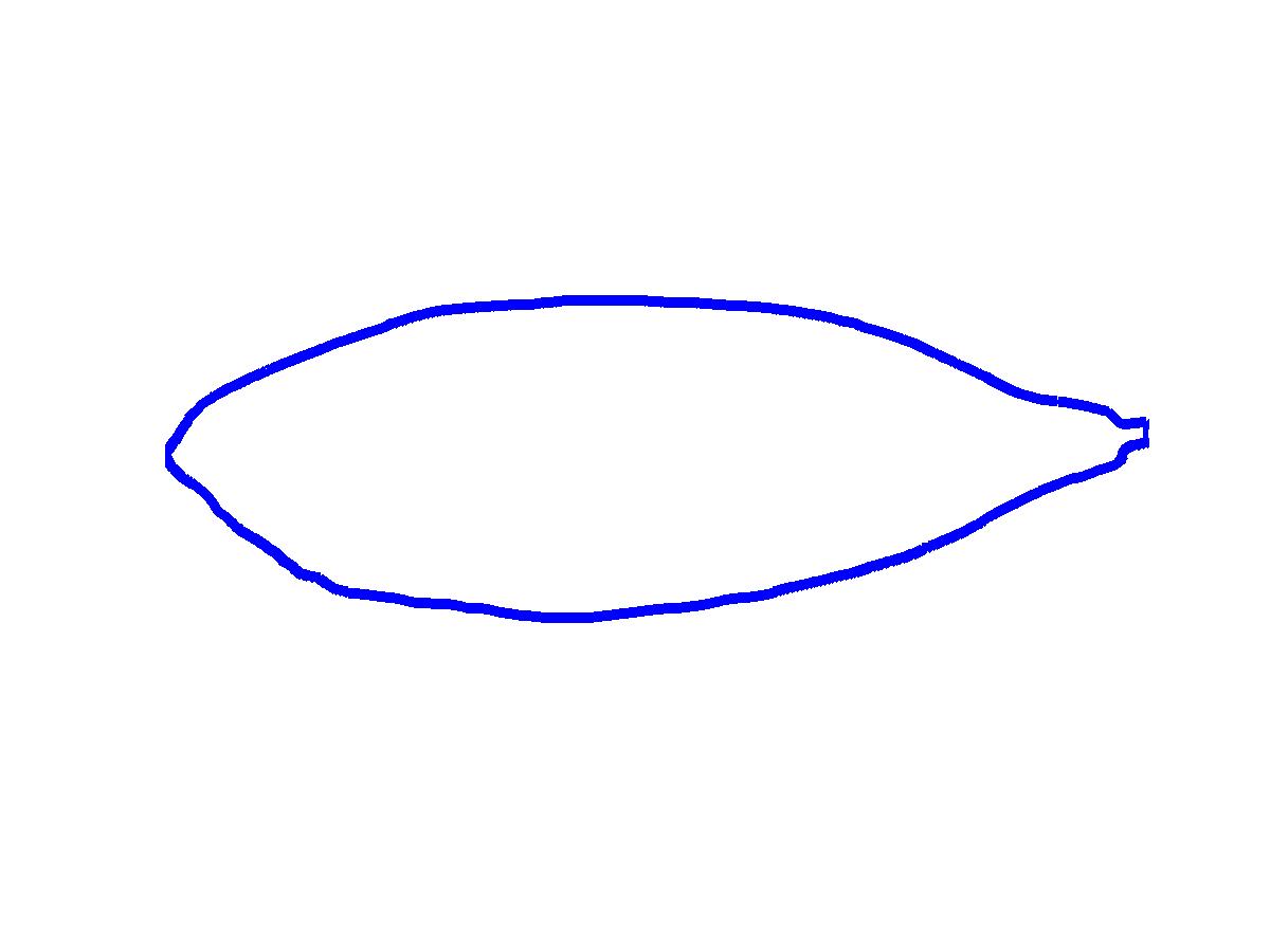
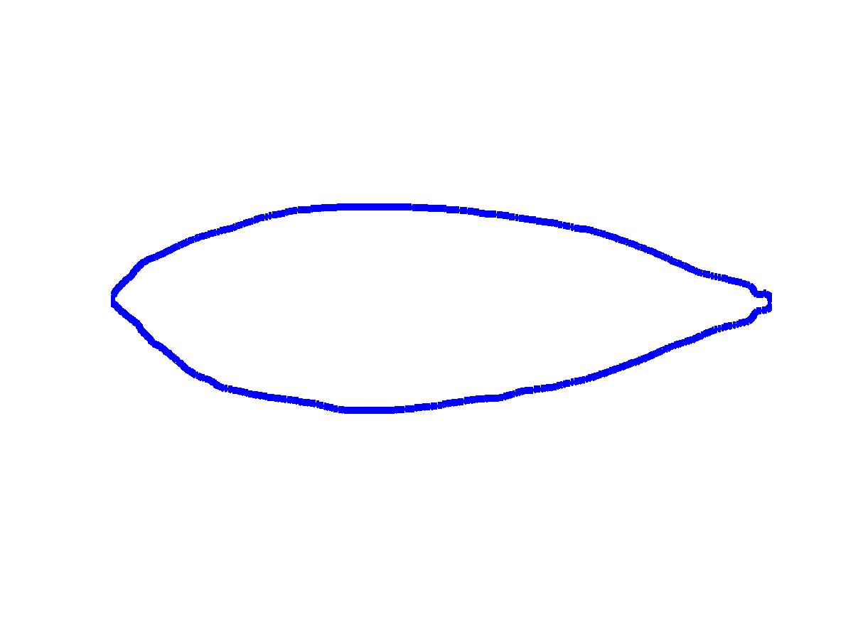
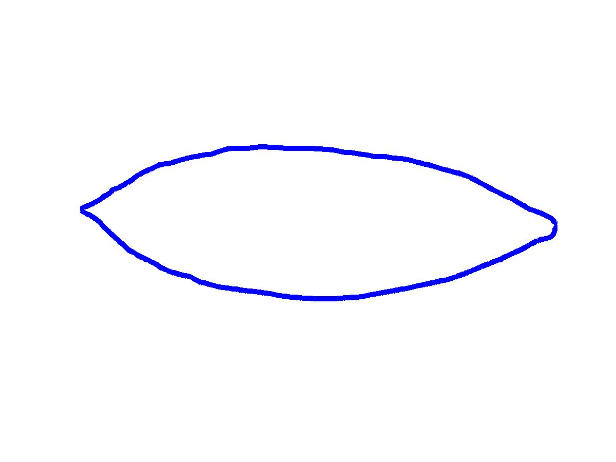
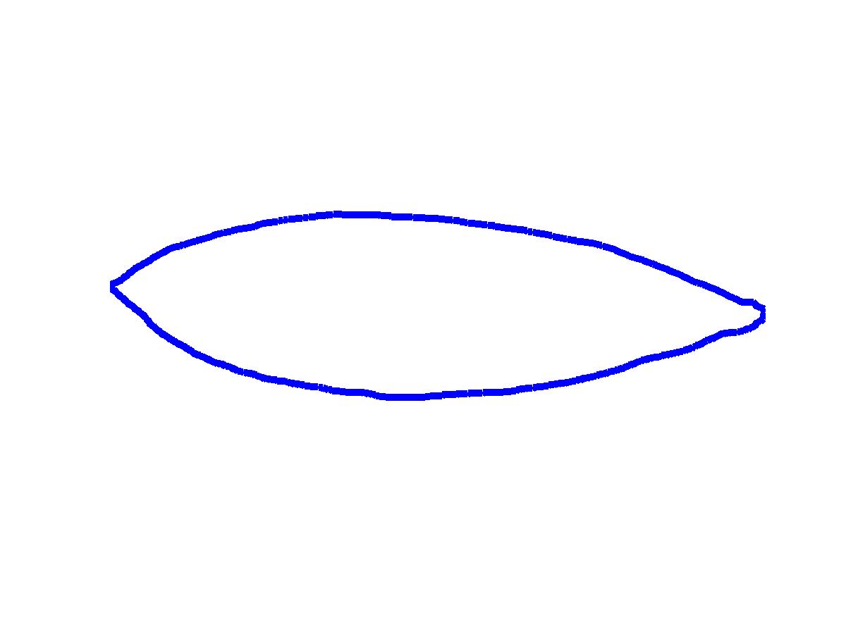
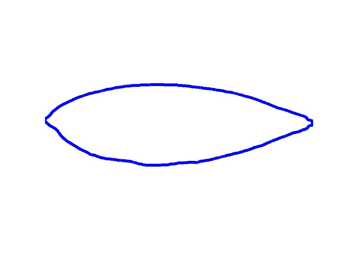
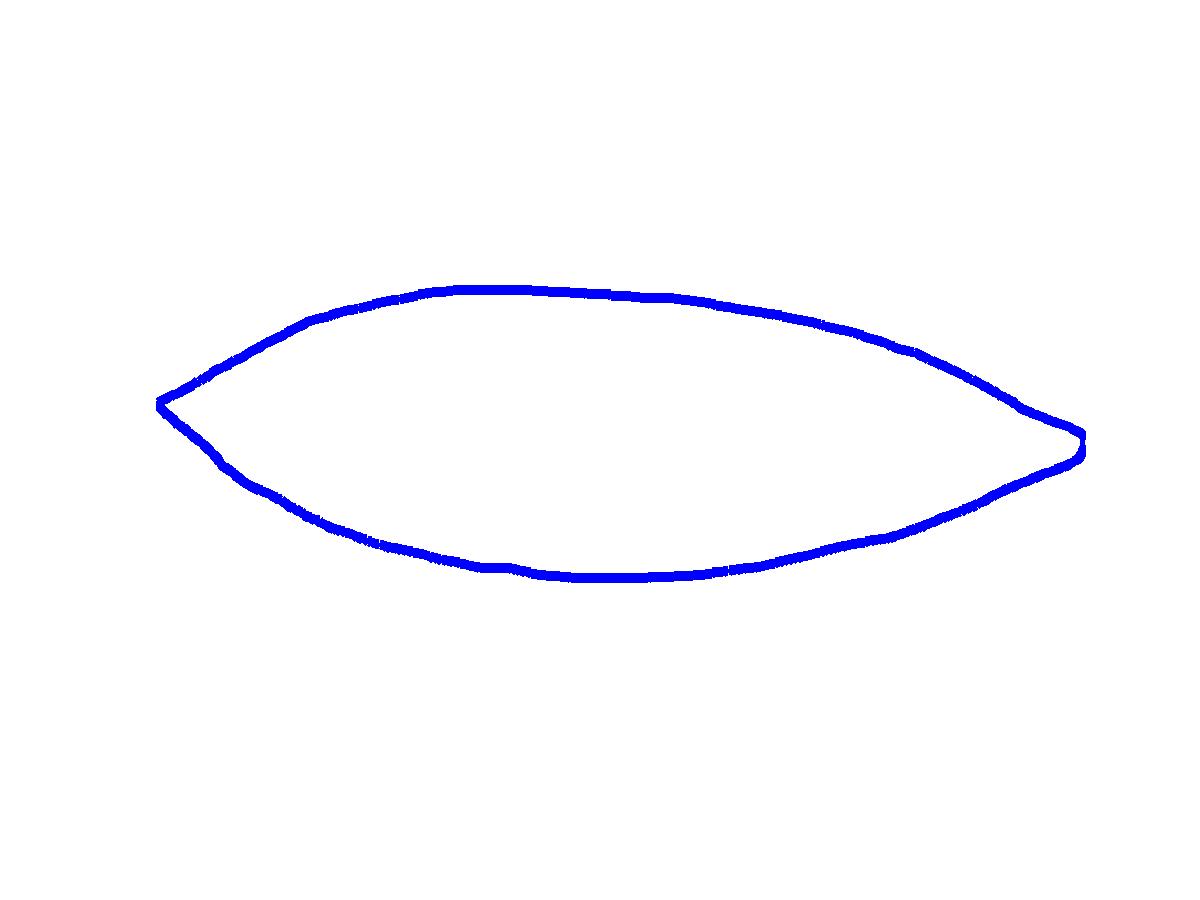
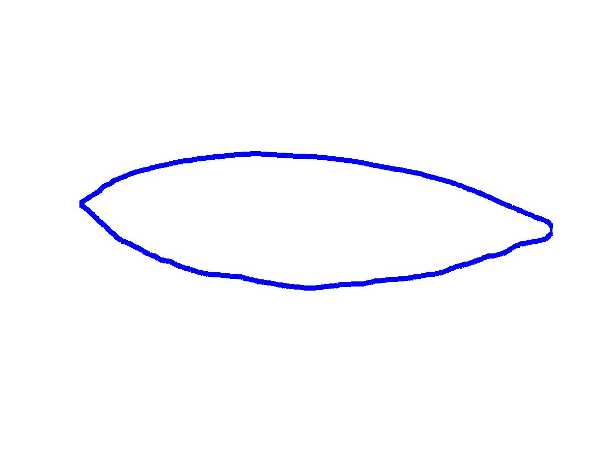
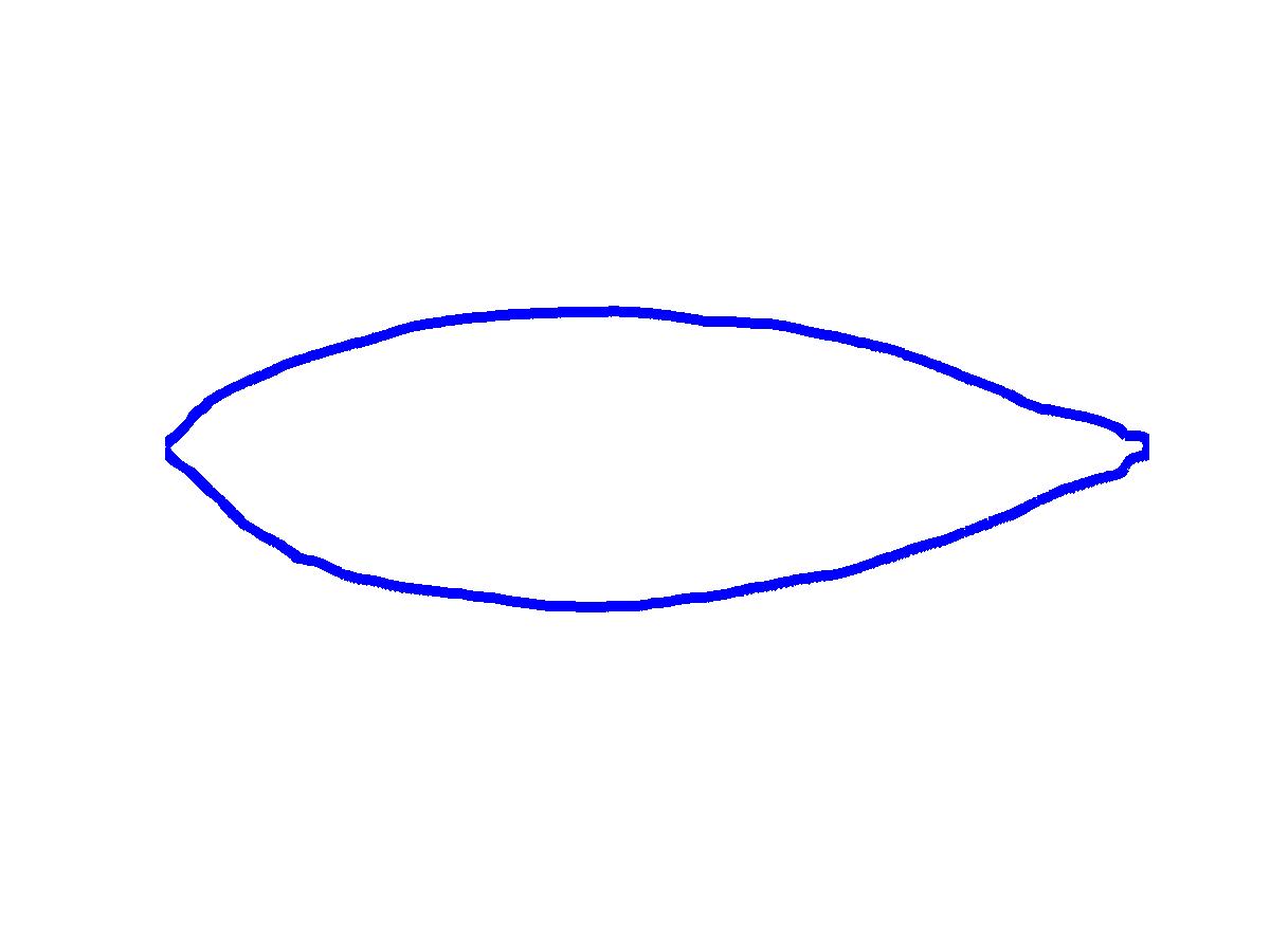
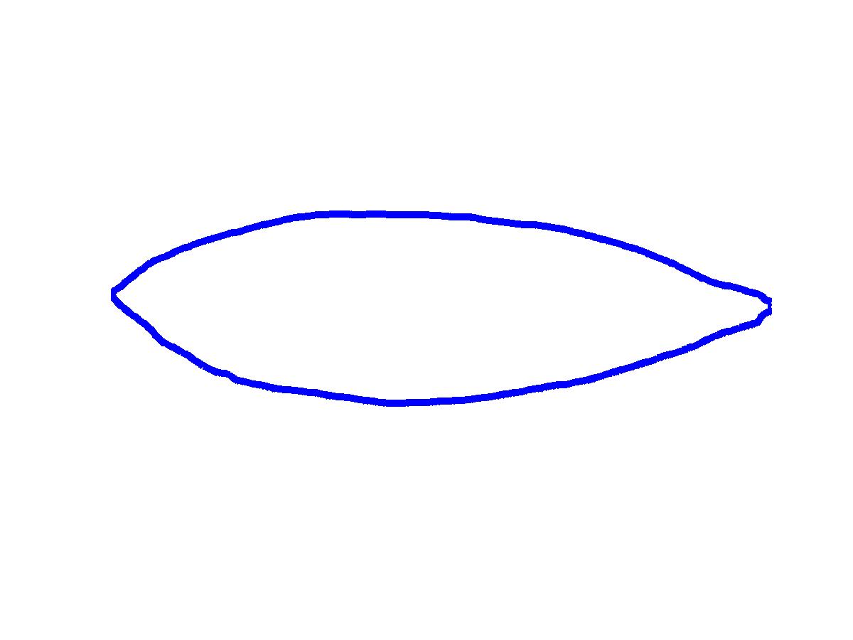
Figure 6: Contours extracted from the original images.

Finally, a neighborhood hypothesis test for a difference in the mean projective shape of the random 3-dimensional contours for leaves A and B was performed and a no significant difference was found. Our TDA analysis which follows outperforms that hypothesis testing procedure developed in Patrangenaru et al. (2016) [43] in terms of (i) being computationally much easier to implement, (ii) yielding statistically more powerful tests which find a significant difference in the leaf A and leaf B images as one would expect and (iii) providing much more information about the topological differences in the leaf image point clouds. Our computations were performed in MATLAB and Image Processing Toolbox Release 2013a, in R-3.4.1 with Pawel Dlotko’s Plot Of Landscapes package [16] and in C++ with Ulrich Bauer’s Ripser code [1]. First edge detection was performed in MATLAB with Sobel, Canny, Prewitt, Roberts, and Log (zero-crossing) methods in the Image Processing toolbox. After an inspection of the results from all five edge detection methods for all 40 point clouds it was found the Log method was essentially the best method in terms of detecting points on the edge or contour and the veins of a leaf and filtering out points not on contour or a vein. The totality of 40 leaf edges, from the Log edge detection method, are shown below in Figure 7.

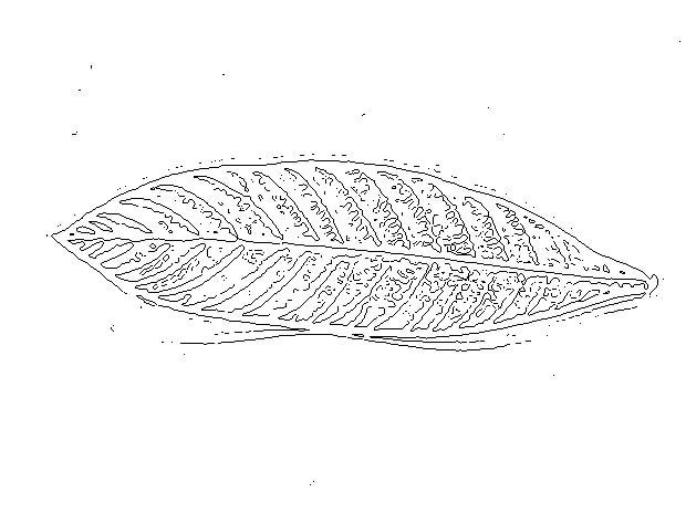
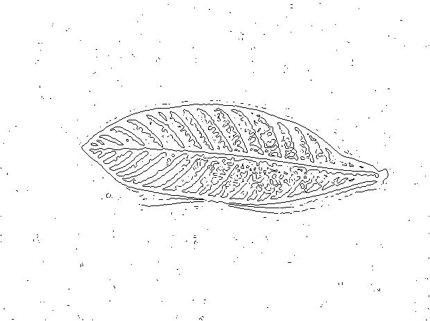
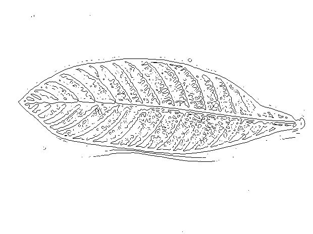
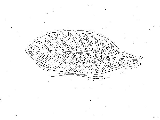
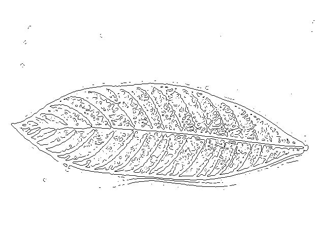
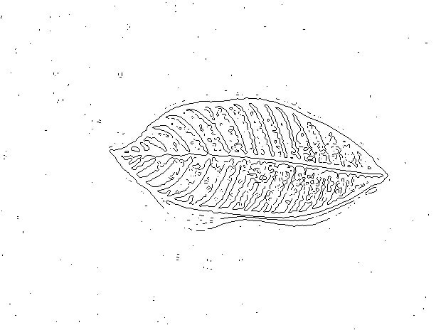
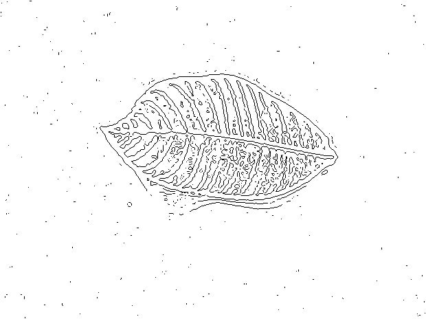
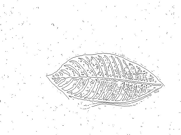
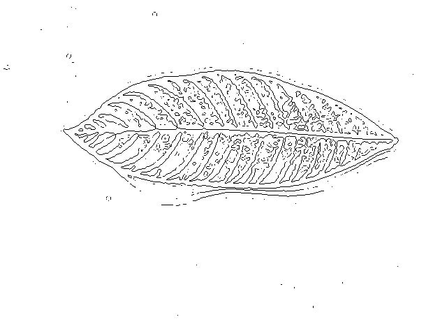
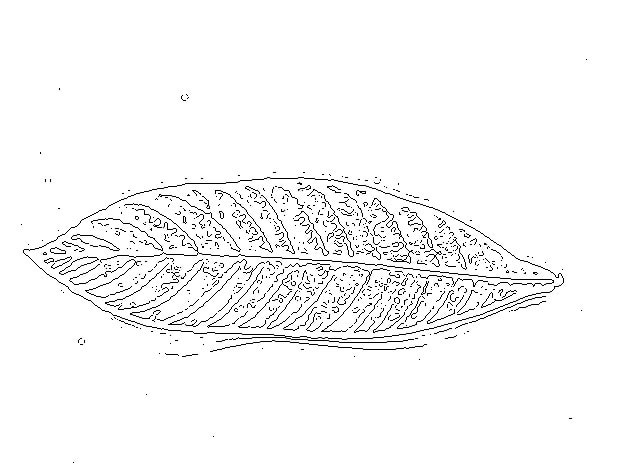
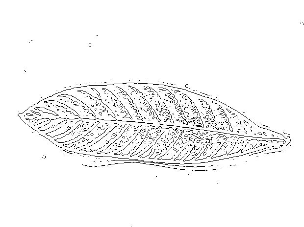
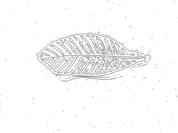
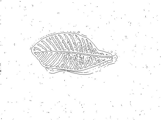
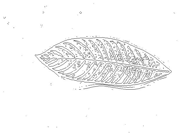
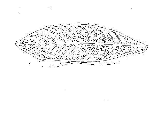
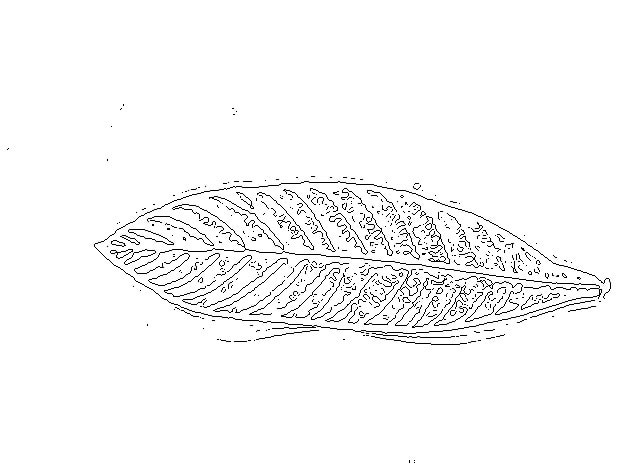
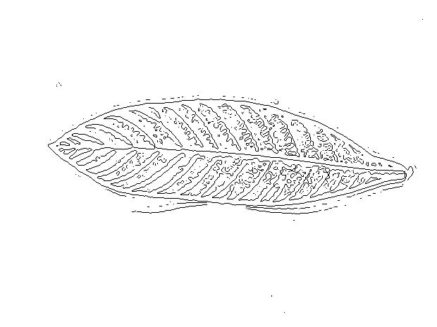
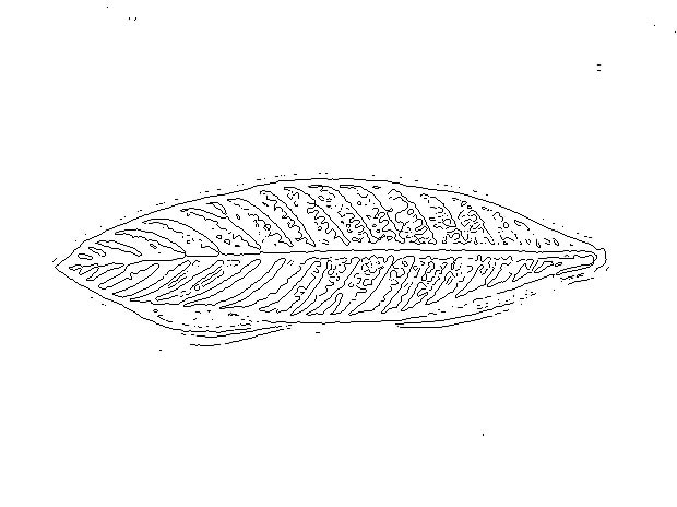
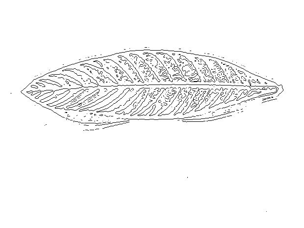
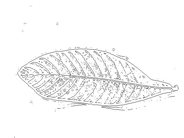
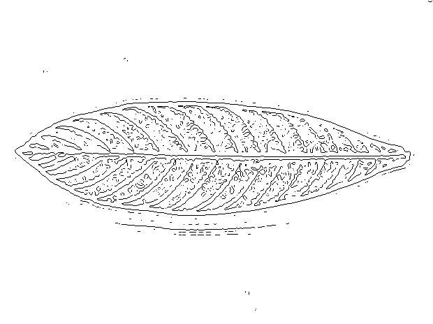
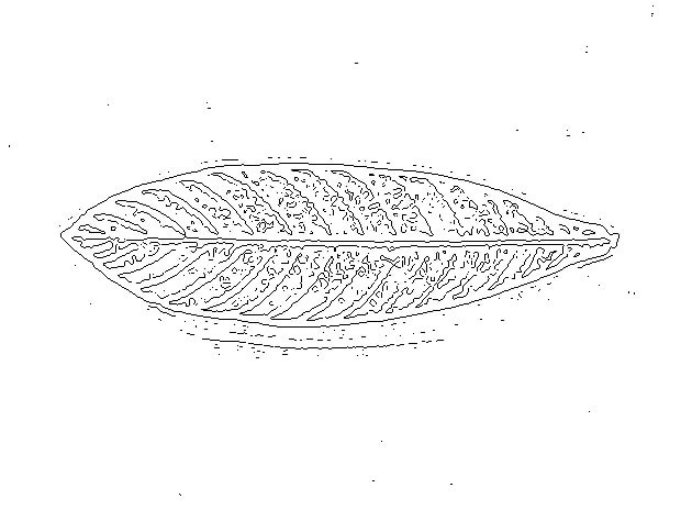
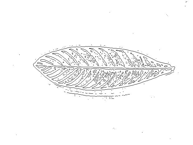
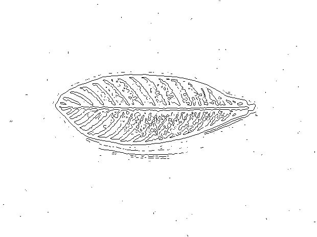
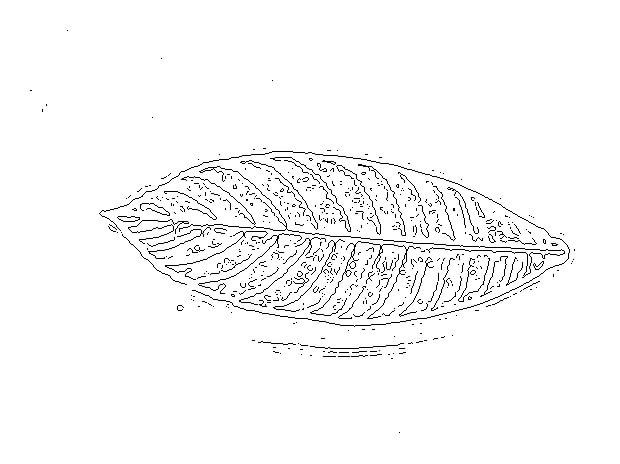
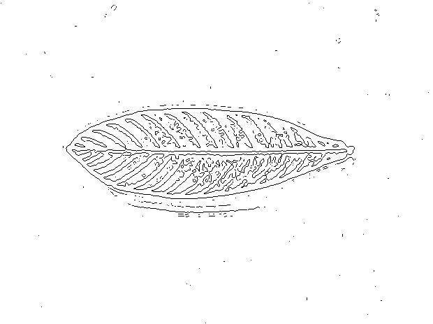
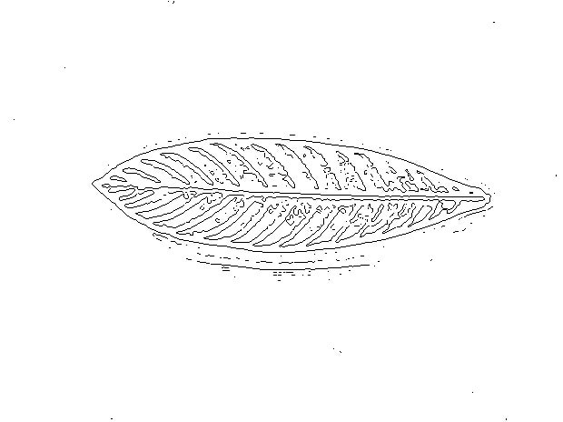
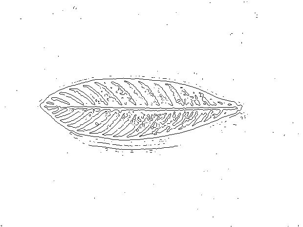
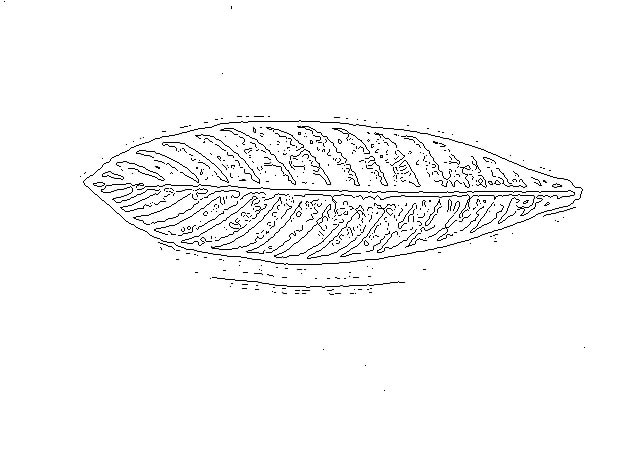
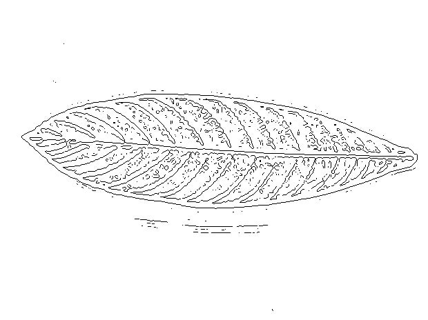
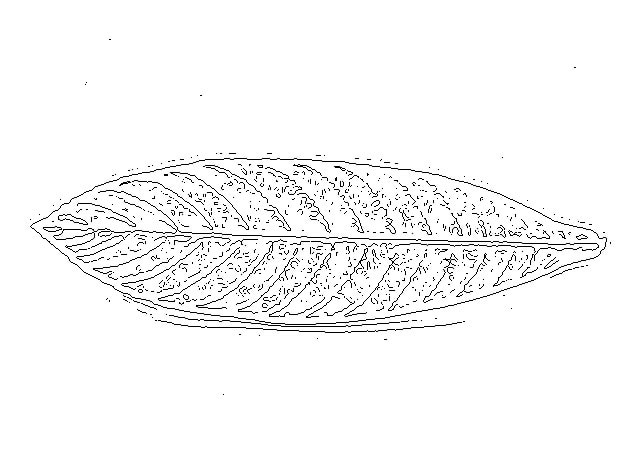
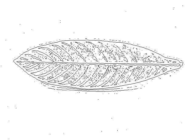
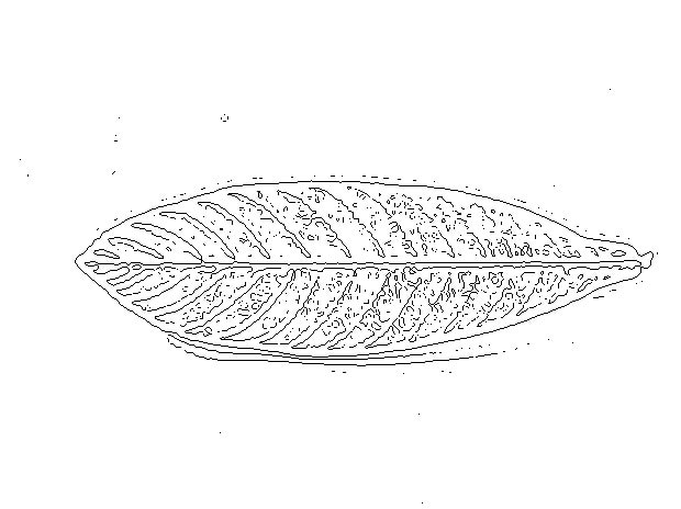
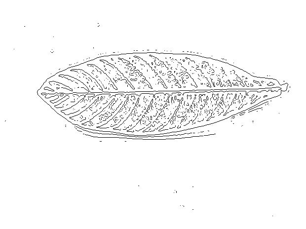
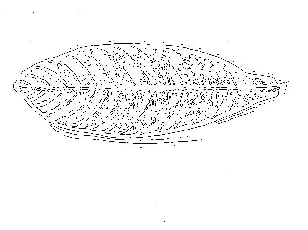
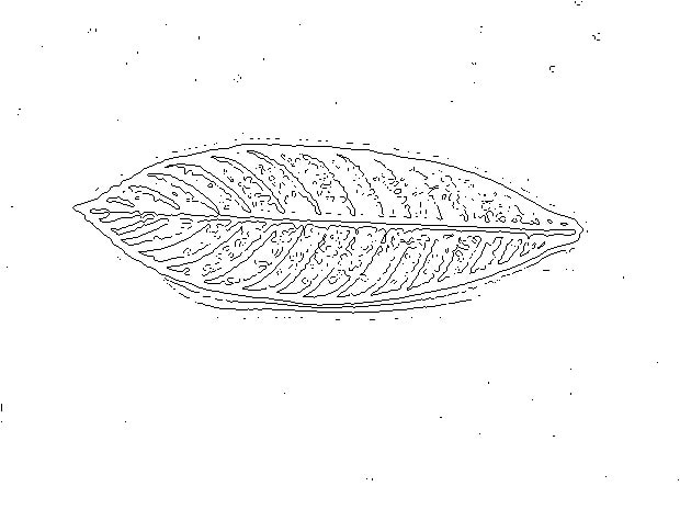
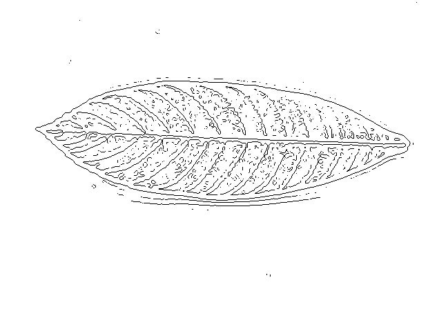
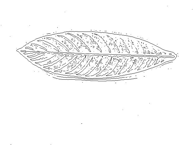
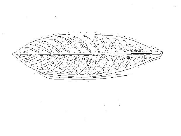
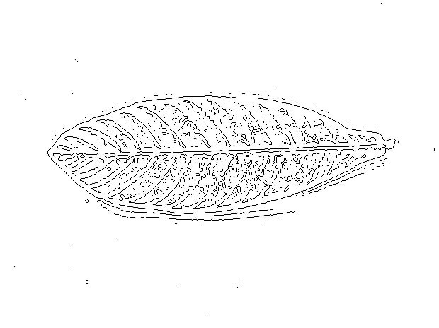
Figure 7: Leaf edges from the original images.

From these leaf edges point clouds consisting of approximately 4300 points were sampled. See Figure 8.

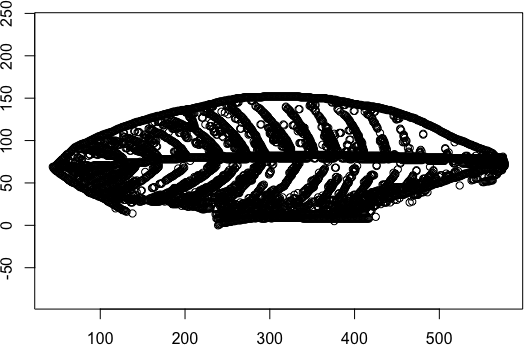
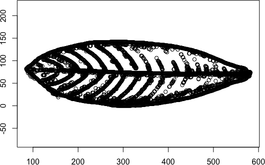
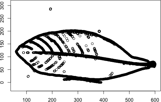
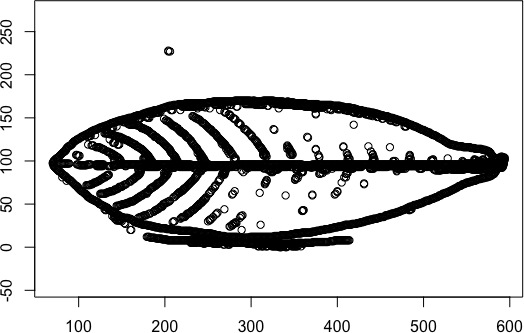
Figure 8: Sample point clouds from leaf A (top left and bottom left) and leaf B (top right and bottom right).

Next, the persistence diagrams for the Vietoris-Rips complexes of all the point cloud data sets were computed using Ripser [1] (see Sections 2.1 and 2.2). These persistence diagrams were then converted into vectors to facilitate statistical analysis. Specifically, the persistence diagrams for homology in degree 0 were converted into death vector (see Section 2.3) and the persistence diagrams for homology in degree 1 were converted into persistence landscapes (see Section 2.2) using the Persistence Landscapes Toolbox [8].

The persistence landscapes were converted into vectors by evaluating on a grid as follows. Specifically, we evaluated the persistence landscape functions $\lambda_{1},\ldots,\lambda_{60}$ (all further landscape functions were identically zero) at the values $0,0.1,0.2,0.3,\ldots,39.9,40$. The resulting $60\times 401=24060$ values were concatenated to obtain vectors in $\mathbb{R}^{24,060}$. For an example of the death vector and the persistence landscape, see Figure 3.

Next, we consider the average death vectors and average persistence landscapes for the two leaves and the differences between these averages. See Figure 9.

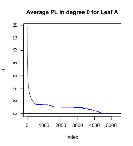
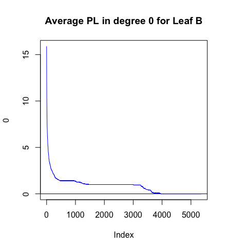
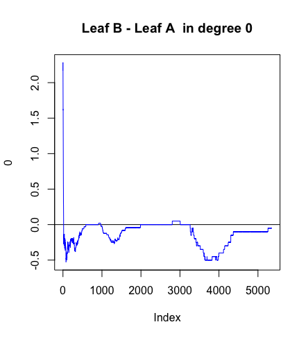
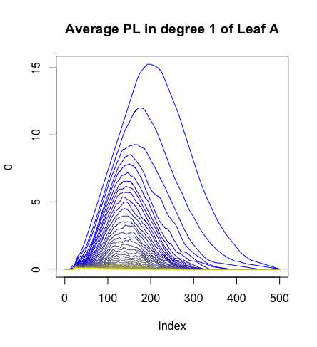
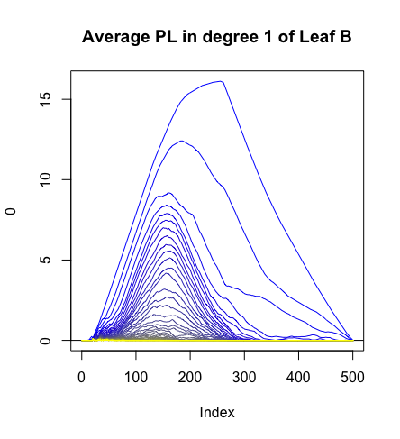
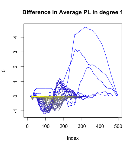
Figure 9: Average death vectors for leaf A (top left) and leaf B (top middle) and their difference (top right). Average persistence landscapes for leaf A (bottom left) and leaf B (bottom middle) and their difference (bottom right).

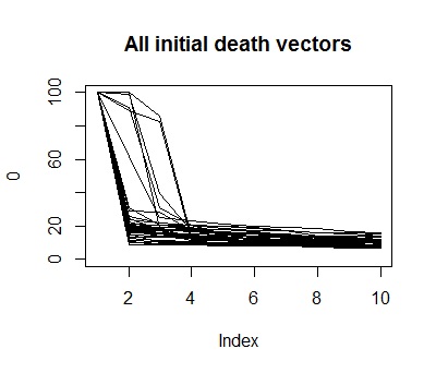
Figure 10: All initial death vectors

Upon inspection, of the initial terms of the death vectors, it was observed that the first three coordinates are very noisy (see Figure 10). As a result, these coordinates were excluded from further statistical analyses (with an eye toward removing “topological noise” from our data to better detect the “geometric signal”), and the resulting permutation test p-value for a difference in the death vectors, of leaves and A and B, was found to be a highly significant 0.0007.

The degree one persistence landscape functions were plotted to look for outliers and none were found. However, that the first 20 or so degree one persistence landscape functions contained large variability and hence large amounts of “topological noise”. In Figure 11, the plots of all of the first two degree one persistence landscape functions are displayed.

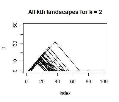
Figure 11: The first (left) and second (right) persistence landscape functions for all of the leaves.

Subsequently, the first 20 degree one persistence landscape functions were excluded (again, to filter out “topological noise”), leaving the remaining degree one persistence landscape functions, and the permutation test p-value for the difference in the lower frequency degree one persistence landscape functions, for leaves and A and B, was found to be highly significant at 0.0019. This p-value is not very sensitive to changing the number of excluded persistence landscape functions. When we did not exclude the first 20 degree one persistence landscape functions then the permutation test p-value was marginally insignificant at 0.0821.

After this we considered classification with support vector machines (SVMs). Here our feature vector was taken to be the death vector concatenated with all degree one persistence landscape vectors. Unlike the statistical analysis, we did not remove any “topological noise”. Using 10-fold cross validation we obtain a fitted classifier with 90% classification accuracy. In fact, we did just as well in terms of classification accuracy when the death vector was removed from the feature vector.

In summary, we see that the points in the persistence diagram that are closest to the diagonal, (that is, the points of high frequency, low variance in our topological statistics) best capture local geometry of the leaves and are better able to distinguish between the two leaves.

4 New Directions in Object Data Analysis

To date, Object Data Analysis (ODA) is the most inclusive type of statistical analysis as far as the complexity of the objects under investigation is concerned. In particular, ODA includes Linear Data Analysis (LDA), shape analysis (see Dryden and Mardia(2016)[18], Patrangenaru and Ellingson(2015)[39]), directional and axial data analysis (see Mardia and Jupp(2000)[34]), data analysis on spaces of phylogenetic trees (see Billera et al(2001)[5]), to mention just a few. Mathematically, ODA is data analysis on an object space, which is a complete separable metric space $(\mathcal{M},\rho)$ and typically has a manifold stratification (see Bhattacharya et al.(2013)[3], Patrangenaru and Ellingson(2015,p.475)[39] and the references therein). A random object is a function $X:\Omega\to\mathcal{M}$ defined on a probability space $(\Omega,\mathcal{A},\mathbb{P})$, such that $X^{-1}(B)\in\mathcal{A},$ for any Borel set $B\in\mathcal{B}_{\rho}$. Let $\mathcal{S}$ be the support of the probability measure (distribution) $Q=\mathbb{P}_{X}$ on $\mathcal{M},Q(B)=\mathbb{P}(X^{-1}(B)),\forall B\in\mathcal{B}_{\rho}.$

The main techniques for a nonparametric analysis of object data are Fréchet function based (see e.g. Patrangenaru and Ellingson (2015)[39]). Since in general there is no group structure on the object space, the total variance of $X$ is defined as the minimum of the expected square distance from $X$ to an arbitrary fixed object $x$ on $\mathcal{M},$ and the minimizers of this Fréchet function (see Fréchet [26]) form the mean set of $X.$ The fastest and theoretically sound quantitative methods for analyzing object data, are extrinsic, based on an object space embedding in a numerical space, with the induced “chord” distance. The embedding also allows using certain linear techniques when testing for equality of two or more distributions on an object spaces, via an extrinsic energy methodology (see e.g. Guo and Patrangenaru(2017)[28]).

4.1 Fréchet Object Data Analysis

Fréchet object data analysis (FODA) is a ODA on a metrizable object space, based on a preferred distance. There are two key types of distances used in FODA: a “chord distance” induced by the Euclidean distance on the numerical space where the object space is embedded, and a geodesic distance associated with a Riemannian structure on the nonsingular part of the object space. Extrinsic FODA (based on the chord distance) has multiple advantages over intrinsic analysis (using a geodesic distance), including computational and methodological advantages (see Bhattacharya et al(2012)[4], Patrangenaru et al(2015, p.168)[39]).

More general location parameters, reflecting the topological structure of both the support of the random object $X$ and of the underlying object manifold $\mathcal{M},$ extending those in Patrangenaru(2016a, 2016b)[40, 41] are introduced below.

Definition 4.

Assume the Fréchet function associated with a random object $X$ on $\mathcal{M}$ is a Morse function (for a definition see eg Bubenik et al [9]). The set of nondegenerate critical points of the Fréchet Morse function $\mathcal{F}_{X}$, with fixed index $r$ is the Fréchet mean set of index $r$ of $X.$

If $\mathcal{M}$ has dimension $m,$ the Fréchet mean sets of index $0$ and $m$ are, respectively, the Fréchet antimean set (see Patrangenaru and Ellingson (2015), p.139), and the Fréchet mean set. In case the Fréchet mean set of index $r$ of $X$ has one point, that point is called Fréchet mean of index $r$ of $X.$ Given a random sample of size $n$ from the distribution $Q$ associated with an random object on $\mathcal{M},$ we define the Fréchet sample mean (set) of index $r$ to be the Fréchet mean (set) of index $r$ of the empirical distribution $\hat{Q}_{n}.$ If the manifold $(\mathcal{M},\rho_{0})$ is compact, where $\rho_{0}$ is the chord distance associated with the embedding $j$ of $\mathcal{M}$ in $\mathbb{R}^{N},$ we define the extrinsic mean (set) of index $r$ of $Q$ to be the Fréchet mean (set) of index $r$ of $Q$ associated with the distance $\rho_{0},$ and given a sample of size $n$ from $Q,$ its extrinsic sample mean (set) of index $r$ is the extrinsic mean (set) of index $r$ of the empirical distribution $\hat{Q}_{n}.$

Remark 5.

Using similar, somewhat more sophisticated techniques as for antimeans (see Patrangenaru et al(2016a)[40]), one may prove the consistency of extrinsic sample means of index $r$ as estimators of the for extrinsic means of index $r$. Along these lines one may also derive the asymptotic distributions for extrinsic sample means of index $r$ that help estimate their population counterparts. To prove consistency, the key new ingredient involves the fact that the class of Morse functions is generic (open and dense).

The new location parameters introduced above allow for an extension of nonparametric regression to extrinsic regression and extrinsic anti-regression, when the response variable is a random object on a compact set. For more details and an application of time dependent anti-regression in projective shape analysis for biological growth of a clam shells species, see Deng et al.(2018)[15]

4.2 Statistical challenges of ODA

Unlike linear data analysis, including functional data analysis, ODA was designed to mainly analyze imaging data, since these days a datum is often an electronic image of some form. Arguably, the most widespread type of imaging data are digital camera images. Among the many challenges arising in with camera images, one of the most difficult is the 3D scene retrieval from its digital camera images (see eg. Ma et al.(2006)[33] or Chapter 22 in Patrangenaru and Ellingson (2015)[39]). If the dimensionality of the scene is of secondary interest, as opposed to its fine structure, as is the case with the TDA leaf data in Section 3, Fréchet function based methods become computationally costly and methodologically challenging. In addition, a plethora of usual methods for random vectors, raise difficulties with random objects on a nonlinear object space. Starting with a proper definition of location and spread parameters as shown in subsection 4.1, dimension reduction, regression, MANOVA and other inference problems, all the way to designing appropriate distributional models on object spaces and designing nonparametric tests for their goodness of fit, one encounters many unanswered, potentially difficult questions. Moreover new challenging questions arising from images of the Universe, on recognising dark matter and singularities as voids in the 3D continuum, raise qualitative questions that can be formulated in more in a TDA setting, rather than a “classical” FODA way. Note that in the multivariate case, Chen et al(2017)[12] already developed TDA techniques for qualitative aspects of data analysis. The challenge is to find similar methods for nonlinear ODA.

4.3 A homology approach to qualitative analysis of distributions on object spaces

From the object data analysis perspective, a closed manifold can be regarded as the support of the distribution on an object space. A basic example is provided by the Fisher von-Mises distribution on $\mathbb{S}^{1}$ [24], whose support is the entire circle. In general any compact manifold $\mathcal{M}$, endowed with a Riemannian structure $g$ may be regarded as the support of a uniform distribution on it, whose density w.r.t. the volume measure is $\frac{1}{Vol_{g}(\mathcal{M})}.$

Remark 6.

A well known result, the topological classification of compact orientable surfaces, shows that an algebraic homology invariant, the rank of the first homology group, which is twice the genus of such a surface, is a classifier for the homeomorphism class of such a surface. In dimensions three, the problem of classifying homeomorphism classes of closed manifolds based on their homology, was advanced only in the eighties and nineties, especially by Thurston-Perelman’s theorem (see Thurston(1982)[47], Perlman [42], Scott(2003)[44], Patrangenaru(1996)[37]), and in dimension four by M.H.Freedman, S. Donaldson and their collaborators (see eg. [17], [25]).

Unfortunately, object data is high dimensional, and in dimensions five or higher, it is way more difficult to classify homeomorphism classes of closed manifolds, even in the smooth case, due to the so called moduli spaces. So, despite the preferred equivalence via homeomorphisms, one has to accept the idea of a weaker form equivalence relation for topological spaces, leading to the notion of homotopy type, which is often used. Intuitively, two topological spaces have the same homotopy type if one can be continuously deformed, but not necessarily in one-to-one correspondence, into the other. The basic definitions are as follows:

Definition 7.

Given two topological spaces $X,Y,$ we say that two continuous functions $F_{0},F_{1}:X\to Y$ are homotopic, and we write $F_{0}\cong F_{1},$ if there is a continuous function $F:[0,1]\times X\to Y,$ such that $\forall x\in X,F(0,x)=F_{0}(x),F(1,x)=F_{1}(x).$ $X$ and $Y$ have the same homotopy type, if there are continuous functions $F:X\to Y,G:Y\to X,$ such that $G\circ F\cong Id_{X},F\circ G\cong Id_{Y}.$

One view of TDA is that it aims to consider the homotopy type of an object or of the support of a distribution, using a random sample of its points in a numerical space. More precisely, it really computes certain invariants associated with the homotopy type, that persist, while gradually inflating this sample by balls of growing radii around them, which is somewhat similar with the recovery of the CW homotopy type of a submanifold $M$ in the Euclidean space, via a filtration by sublevel sets of a Morse function (see Bubenik et al.(2010)[9]). Persistent homology measures these invariants associated with the homotopy type of the “telescoping” limit via this filtration $M_{n},n\in\mathbb{N}$ of $M$. Essentially if $\mathcal{S}$ is regarded as a union of sub-level level sets $\mathcal{S}_{n}$ of the support of a probability distribution on $\mathbb{R}^{p},$ one may consider the homotopy type of $(\mathbb{R}^{p},\mathcal{S}_{n}),$ as an “estimate” of the homotopy type of the pair $(\mathbb{R}^{p},\mathcal{S}).$ Note that two pairs $(\mathbb{R}^{p},A_{1}),(\mathbb{R}^{p},A_{2}),$ have the same homotopy type, if there are continuous functions $h,k:\mathbb{R}^{p}\circlearrowleft,$ with $h(A_{1})\subseteq A_{2},k(A_{2})\subseteq A_{1},$ such that $h\circ k$ and $k\circ f$ are homotopic to the identity of $\mathbb{R}^{p}.$ Thus within the same homotopy type, the continuity relation between the contiguous regions and the number of holes or voids of the subspaces $A_{1},A_{2}$ of $\mathbb{R}^{p}$ remains unchanged. Furthermore, when it comes to the support $\mathcal{S}$ of a distribution on an object space $\mathcal{M},$ this continuity relation of the pair $(\mathcal{M},\mathcal{S})$ is reflected by the homology of the pair $(\mathcal{M},\mathcal{S}),$ more precisely, its algebraic consequence, the exact homology sequence of this pair (see Patrangenaru and Ellingson (2015)[39], p.131-132). Homology is our approach to studying the support of a distribution, unlike homotopic trees that used for understanding connections (or continuity) between the contiguous connected components in machine vision (eg Sonka et al.(2015)[46], p.699, and an illustration in the Figure 12 below).

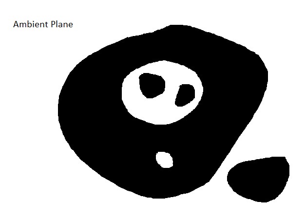
Figure 12: Contiguity of connected components explained via a homotopic tree.

4.4 Topological Object Data Analysis

Given the pair $(\mathcal{M},\mathcal{S}),$ where $\mathcal{M}$ is the ambient object space and $\mathcal{S}$ is the support of a distribution on $\mathcal{M},$ there is a long exact sequence in homology, via the inclusions $i:\mathcal{S}\to\mathcal{M}$ and $j:\mathcal{M}\to(\mathcal{M},\mathcal{S}),$ where $\mathcal{M})$ is the shorthand for $(\mathcal{M},\emptyset):$

$$\cdots\to H_{k}(\mathcal{S})\to^{{\!\!\!\!\!\!i_{k}}}H_{k}(\mathcal{M})\to^{{\!\!\!\!\!\!j_{k}}}H_{k}(\mathcal{M},\mathcal{S})\to^{{\!\!\!\!\!\!\partial_{k}}}H_{{k-1}}(\mathcal{S})\to\cdots.$$ (1)

Topological Object Data Analysis (TODA) is a data driven homology based statistical analysis of the relative homology spaces $H_{k}(\mathcal{M},\mathcal{S}).$

Note that since the homology groups of the Euclidean space are all trivial, except for $H_{0}(\mathbb{R}^{m})=\mathbb{Z},$ from (1) it follows that in case of a random vector $X$, $H_{k}(\mathcal{M},\mathcal{S})\backsimeq H_{k-1}(\mathcal{S}),$ therefore TODA aims at estimating the homology of $\mathcal{S},$ for example via a persistent homology.

Some stratified spaces of interest like spaces $T_{k}$ of phylogenetic trees with $k$ leafs (see Billera et al(2001)[5]) are contractible, therefore they have trivial reduced homology as well, thus for any random phylogenetic tree $X$ with $k$ leafs, whose distributional support is $\mathcal{S},$ the relative homology $H_{k}(T_{k},S)\backsimeq H^{k-1}(S),$ similar with the case of a random vector. From this perspective, TODA applies to phylogenetic tree spaces, via persistence homology techniques. This opens a new venue to qualitative analysis for certain types of Big Data.

References

- [1] Bauer, Ulrich (2017). Ripser: a lean C++ code for the computation of Vietoris–Rips persistence barcodes. Software available at https://github.com/Ripser/ripser.
- [2] Bendich, Paul; Marron, J. S.; Miller, Ezra; Pieloch, Alex; Skwerer, Sean. (2016). Persistent homology analysis of brain artery trees. Ann. Appl. Stat. 10, 198-–218.
- [3] Rabi N. Bhattacharya, Marius Buibas, Ian L. Dryden, Leif A. Ellingson, David Groisser, Harrie Hendriks, Stephan Huckemann, Huiling Le, Xiuwen Liu, James S. Marron, Daniel E. Osborne, Vic Patrângenaru, Armin Schwartzman, Hilary W. Thompson, and Andrew T. A.Wood. (2013) Extrinsic data analysis on sample spaces with a manifold stratification. Advances in Mathematics, Invited Contributions at the Seventh Congress of Romanian Mathematicians, Brasov, 2011, Publishing House of the Romanian Academy (Editors: Lucian Beznea, Vasile Brîzanescu, Marius Iosifescu, Gabriela Marinoschi, Radu Purice and Dan Timotin), pp. 241–252.
- [4] R. N. Bhattacharya, L. Ellingson, X. Liu and V. Patrangenaru and M. Crane (2012). Extrinsic Analysis on Manifolds is Computationally Faster than Intrinsic Analysis, with Applications to Quality Control by Machine Vision. Applied Stochastic Models in Business and Industry. 28, 222-235.
- [5] Billera, L., Holmes, S., Vogtmann, K.(2001). Geometry of the space of phylogenetic trees. Adv. Appl. Math. 27, 733–-767.
- [6] Bubenik, P. and Kim, P.T. (2007). A Statistical Approach to Persistent Homology, Homology, Homotopy and Applications, , .
- [7] Peter Bubenik.(2015). Statistical Topological Data Analysis using Persistence Landscapes. J. of Machine Learning Research. 16, 77–102.
- [8] Peter Bubenik and Pawel Dlotko (2017). A persistence landscapes toolbox for topological statistics.A persistence landscapes toolbox for topological statistics. 78, 91 – 114.
- [9] Bubenik, Peter; Carlsson, Gunnar; Kim, Peter T. and Luo, Zhi-Ming.(2010). Statistical topology via Morse theory persistence and nonparametric estimation. Algebraic methods in statistics and probability II, 75–-92, Contemp. Math., 516, Amer. Math. Soc.
- [10] Chazal, F., Oudot, S., Marc Glisse, M. and De Silva, V. (2016). The Structure and Stability of Persistence Modules. Springer Briefs in Mathematics pp.VII, 116, Springer-Verlag
- [11] Chazal, F., Fasy, B.T., Lecci, F., Michel, B., Rinaldo, A. and Wasserman, L. (2014). Robust Topological Inference: Distance-To-a-Measure and Kernel Distance. Technical Report
- [12] Chen, Yen-Chi; Genovese, Christopher R.; Wasserman, Larry.(2017). Statistical inference using the Morse-Smale complex. Electron. J. Stat. 11, 1390–-1433
- [13] Cohen-Steiner, David; Edelsbrunner, Herbert and Harer, John.(2007). Stability of persistence diagrams. Discrete Comput. Geom., 37, 103–120.
- [14] De Silva, V., Morozov, D. and Vejdemo-Johansson, M. (2011) Persistent Cohomology and Circular Coordinates, Discrete and Computational Geometry 45 737-759.
- [15] Y. Deng, V. Patrangenaru and V. Balan (2017). Anti-regression on Manifolds with an Applications to 3D Projective Shape Analysis. BSG Proceedings, 25, (In press).
-
[16]
Dlotko, Pavel.(2018). The Persistent Ladscape Toolbox
https://www.math.upenn.edu/dlotko/persistenceLandscape.html - [17] Donaldson, S. K.; Kronheimer, P. B.(1990). The geometry of four-manifolds. Oxford Mathematical Monographs. Oxford Science Publications. The Clarendon Press, Oxford University Press, New York.
- [18] Dryden, I.L. and Mardia, K.V. (2016). Statistical Shape Analysis, with Applications in R. Second Edition. Wiley, Chichester.
- [19] Edelsbrunner, H. and Harer, J. Persistent Homology- a Survey. Surveys on Discrete and Computational Geometry. Twenty Years Later, eds. J.E. Goodman, J. Pach and R. Pollack, Contemporary Mathematics , Amer. Math. Soc., Providence, Rhode Island,
- [20] Edelsbrunner, Herbert; Harer, John L.(2010). Computational topology. An introduction. American Mathematical Society, Providence, RI. ISBN: 978-0-8218-4925-5
- [21] L. Ellingson, F. H. Ruymgaart and V. Patrangenaru (2013). Nonparametric Estimation of Means on Hilbert Manifolds and Extrinsic Analysis of Mean Shapes of Contours. Journal of Multivariate Analysis. 122, 317–333.
- [22] Fasy, B.T., Lecci, F., Rinaldo, A., Wasserman, L., Balakrishnan, S. and Singh, A. (2014) Statistical Inference For Persistent Homology: Confidence Sets For Persistence Diagrams, Annals of Statistics. Ann. Statist., , .
- [23] Fasy, B.T., Jisu Kim, J., Lecci, F. and Maria, C. (2015). Introduction to the R package TDA.
- [24] Fisher, N. I. (1983). Statistical analysis of circular data. Cambridge University Press, Cambridge.
- [25] Freedman, Michael H.; Quinn, Frank (1990). Topology of 4-manifolds. Princeton Mathematical Series, 39. Princeton University Press, Princeton, NJ.
- [26] Fréchet, M.(1948). Les élements aléatoires de nature quelconque dans un espace distancié (In French). Ann. Inst. H. Poincaré, 10, 215–310.
- [27] Ghrist, R.(2008). Barcodes: The Persistent Topology of Data, Bulletin of the American Mathematical Society, 45, .
- [28] R. Guo and V. Patrangenaru (2017). Testing for the Equality of two Distributions on High Dimensional Object Spaces. arXiv:1703.07856.
- [29] Izenman, A. J. (2008). Modern Multivariate Statistical Techniques: Regression, Classification, and Manifold Learning, Springer, New York.
- [30] Jaco, William H.; Shalen, Peter B. (1979). Seifert fibered spaces in 3-manifolds. Mem. Amer. Math. Soc. 21 , no. 220
- [31] Kaczynski, T., Mischaikow, K., and Mrozek, M. Algebraic Topology: A Computational Approach. Lecture Notes.
- [32] Kovacev-Nikolic, V; Bubenik P., Nikolic, D. and Heo, G. (2016). Using persistent homology and dynamical distances to analyze protein binding. Stat. Appl. Genet. Mol. Biol. 15(1), .
- [33] Ma, Y., Soatto, S., Kosecka, J. and Sastry, S.S. (2006). An invitation to 3-D vision, Springer, New York.
- [34] Mardia, K. V. and Jupp, P.E.(2000). Directional Statistics, Wiley, Chichester.
- [35] Mielke, P.W. and Berry, K.J. (2001). Permutation Methods: A Distance Function Approach, Springer, New York.
- [36] J. Milnor (1962). A unique decomposition theorem for 3-manifolds, American Journal of Mathematics, 84
- [37] Patrangenaru, V.(1996). Classifying 3- and 4-dimensional homogeneous Riemannian manifolds by Cartan triples. Pacific J. Math. 173, no. 2, 511–532
- [38] P Niyogi, S Smale, S Weinberger. (2008) Finding the homology of submanifolds with high confidence from random samples. Discrete Computational Geometry 39, 419–441.
- [39] Patrangenaru, V. and Ellingson, L. E. (2015). Nonparametric Statistics on Manifolds and their Applications to Object Data Analysis. CRC.
- [40] V. Patrangenaru, K.D.Yao and R. Guo (2016a). Nonparametric Inference for Location Parameters via Fréchet Functions. 2nd International Symposium on Stochastic Models in Reliability Engineering, Life Science and Operations Management (SMRLO), Beer Sheva, Israel. ( Edited by Frenkel, I and Lisnianski, A) 254–262.
- [41] V. Patrangenaru, K.D.Yao and R. Guo (2016b). Extrinsic Means and Antimeans. In: Cao R., González Manteiga W., Romo J. (eds) Nonparametric Statistics. Springer Proceedings in Mathematics Statistics, vol 175. 161–178.
- [42] Perelman, G. (2003) Ricci Flow with Surgery on Three-Manifolds, http://arxiv.org/abs/math.DG/0303109.
- [43] V. Patrangenaru, R. Paige, K. D. Yao, M. Qiu and D. Lester (2016). Projective Shape Analysis of Contours and Finite 3D Configurations from Digital Camera Image. Statistical Papers. 57, 1017–1040.
- [44] Scott, Peter (1983). The geometries of 3-manifolds. Bull. London Math. Soc. 15, no. 5, 401–487.
- [45] Soille, P. (2003). Morphological Image Analysis: Principles and Applications, Springer-Verlag New York.
- [46] Milan Sonka, Vaclav Hlavac, Roger Boyle (2015). Image Processing, Analysis, and Machine Vision , 4th Edition.
- [47] Thurston, William P. (1982). Three-dimensional manifolds, Kleinian groups and hyperbolic geometry. Bull. Amer. Math. Soc.(NS) .6, no. 3, 357–-381.