Towards the ICRF3: astrometric comparison of the USNO 2016A VLBI solution with ICRF2 and Gaia DR1

Abstract

The VLBI USNO 2016A (U16A) solution is part of a work-in-progress effort by USNO towards the preparation of the ICRF3. Most of the astrometric improvement with respect to the ICRF2 is due to the re-observation of the VCS sources. Our objective in this paper is to assess U16A’s astrometry. A comparison with ICRF2 shows statistically significant offsets of size 0.1 mas between the two solutions. While Gaia DR1 positions are not precise enough to resolve these offsets, they are found to be significantly closer to U16A than ICRF2. In particular, the trend for typically larger errors for Southern sources in VLBI solutions are decreased in U16A. Overall, the VLBI-Gaia offsets are reduced by 21%. The U16A list includes 718 sources not previously included in ICRF2. Twenty of those new sources have statistically significant radio-optical offsets. In two-thirds of the cases, these offsets can be explained from PanSTARRS images.

=1 Friends of AASTeX

1 Introduction

The ICRF2 catalog (Fey et al., 2015) is the current realization of the International Celestial Reference Frame (ICRF) since 2010. This paper discusses some of the work done in preparation of the future iteration of the ICRF, the ICRF3. Most of the current improvement discussed in this paper comes from the re-observation of the VCS sources (VCS-II, see Gordon et al. (2016)).

In the optical domain, the Gaia mission already produced astrometrically unmatched positions of the ICRF2 optical counterparts in its first data release (Lindegren et al., 2016). In particular, Mignard et al. (2016) investigated the distribution of offsets between ICRF2 and the Gaia Auxiliary Quasar Solution; they found that the bulk of the sources have a scatter of $\sim 1.5-1.8$ mas in the coordinates for the whole sample and $\sim 0.7$ mas for the defining sources. They also found a significant bias of -0.1 mas in declination (in the sense Gaia - ICRF2) for the defining subset.

While the ICRF2 is built uniquely on S/X observations, recent efforts with observations in the K-band give solutions closer to GAIA DR1 (Jacobs et al., 2017), and are thus already a significant improvement to the ICRF2, even with the limited number of sources observed up to now. This makes the contribution of K-band observations highly compelling for the future of the ICRF.

Many works have discussed the presence of offsets between the radio and optical positions (see for example Assafin et al. (2013); Orosz & Frey (2013); Zacharias & Zacharias (2014)). The offsets can give some information on the intrinsic structure of the source, such as the presence of a jet structure (Kovalev et al., 2017). Several papers recently investigated the statistically significant radio-optical offsets using radio positions and the larger secondary solution of the Gaia DR1 catalog (Petrov & Kovalev, 2017a; Makarov et al., 2017). Makarov et al. (2017) investigated the statistically significant offsets between ICRF2 and Gaia DR1 and used PanSTARRS (Chambers et al., 2016) images to find, when possible, the underlying reason; close doubles (actual binaries or chance alignements with field stars), source confusion or extended objects. Knowledge of the large offsets is important as they can complicate the astrometric adjustment of large catalogs to the ICRF (see Berghea et al. (2016) for a discussion of this issue).

This paper discusses the astrometric differences between the work-in-progress toward ICRF3 developed at USNO, called USNO 2016A (hereafter named U16A), the ICRF2, and the Gaia DR1 catalog.

2 The USNO 2016A Global CRF Solution

The United States Naval Observatory is one of the VLBI Analysis Centers for the International VLBI Service (IVS) and as such, is responsible for producing Celestial and Terrestrial Reference Frame (CRF and TRF, respectively) products for the community. Here, we present the U16A global solution for the CRF derived using observations that date back to the onset of the astrometric/geodetic VLBI in 1979. Data were acquired at standard wavelengths of 13 and 3.6 cm simultaneously; this allows for accurate calibration of the wavelength-dependent propagation delays introduced by the Earth’s ionosphere. VLBI astrometry uses multiple channels within each band and applies a least-squares analysis method in order to produce precise group delays. Typically, VLBI observing sessions occur over a 24-hour period, which is necessary to separate the parameters for polar motion and nutation. The U16A solution was determined using the CALC/SOLVE software currently distributed by Goddard Space Flight Center (GSFC). For a comprehensive description of the least-squares method used for deriving source positions from group delay observations, we refer to Ma et al. (1986).

The U16A solution contains a total of 4129 sources, 295 of which are part of the “defining sources” category of VLBI sources. These 295 objects have been observed with the highest number of observing sessions and thus, have the most constrained positions in the solution. There are 2195 sources that are part of the VLBA Calibrator Survey (VCS) as presented in Beasley et al. (2002), which have since been re-observed. These VCS sources are among the least observed objects in the solution with a median number of observing sessions of only two and therefore, have the least constrained positions. The remaining objects are a mixture of new and other, non-VCS sources. The U16A solution contains 3411 objects from the ICRF2. Three ICRF2 sources are absent from the U16A solution: SN1993J, VELA, and LANA. Table 1 summarizes the different sources and the number of times the objects have been observed. In the next section, we compare the differences in position between the U16A solution and the ICRF2.

Type of source	Number	Number of sessions			Number of observations (delays)
		min	median	max	min	median	max
Defining	295	27	190	4398	104	4376	385497
VCS	2195	1	2	34	12	113	674
Non-VCS	921	1	16	3830	3	214	234292
New	718	1	2	18	3	59	864
Total	4129	1	2	4398	3	111	385497

Table 1: Statistics of the U16A solution

3 Comparison of the U16A solution with ICRF2

Figure 1 shows the differences U16A-ICRF2 for both coordinates. We can already notice a clear systematic difference in the declination component. Table 2 gives the median differences in components and absolute offsets. The numbers between parentheses are the confidence intervals of the median, computed with bootstrap resampling (Efron & Tibshirani, 1994), using the BC_a (Bias-Corrected and accelerated) intervals (DiCiccio & Efron, 1996) with 95% coverage and 20,000 bootstrap samples. The advantage of using the bootstrap here is to i) provide a statistical uncertainty for the median estimator, and ii) compute that uncertainty without assuming any error distribution. We will study the consistency of the U16A formal errors in a later section.

Figure 1: Position differences in mas, in the sense U16A-ICRF2, restricted to the range [-1,1] mas.

	295 defining		2191 VCS		921 Non-VCS		3407 sources
RA*cos(Dec)	-9	(-24, 12)	-31	(-49, -7)	-3	(-19, 4)	-17	(-25, -4)
Dec	-45	(-60, -35)	-27	( -55, -6)	-42	(-52, -35)	-39	(-50, -31)
Angular separation	90	(79, 100)	572	(517, 618)	141	(129, 150)	306	(286, 328)

Table 2: Median differences in position in the sense U16A-ICRF2, in $\mu$as. The number between parentheses are bootstrap BC_a confidence intervals with 95% coverage. The median differences in both coordinates represent the systematic offset between the solutions, while the median angular separation gives a sense of the scatter of the absolute displacement.

The median of the absolute offsets between the two solutions is $\sim$ 0.3 mas. However the differences are heterogeneous when we consider the different subsets and components. There is a clear difference in declination for the defining and non-VCS sources between the two catalogs, while the VCS subset seems less affected. As noted above, a 0.1 mas offset was similarly reported by Mignard et al. (2016) in a comparison between Gaia AQS and ICRF2. In comparison, the differences in RA*cos(Dec) are much less sharp, and the only statistically significant difference concerns the VCS sources.

The behavior of the offsets with respect to the right ascension and declination is shown on figure 2, where we only show the trends that indicate a significant, non-linear behavior with respect to the components. The blue line indicates a local robust average, while the green lines represent a 95% confidence interval computed with bootstrap resampling. Details on the statistical method are given in the appendix. One of the main features is a clear negative systematic offset in the declination, mostly affecting the southern declinations for the defining and non-VCS subsets and peaking at $\delta\sim$ - 30 deg.

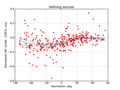
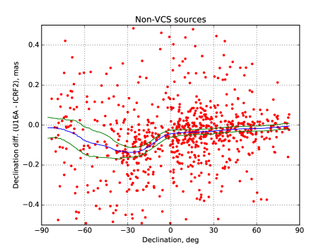
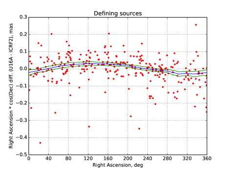
Figure 2: Position differences in mas, in the sense U16A-ICRF2. The blue curve is a robust local estimate of the mean, while the green curves indicate its 95% confidence interval. See appendix A for details.

Another distinct, though smaller, feature is a sinusoidal pattern of the right ascension offset with respect to that same coordinate for the defining sources.

Finally, we note that there are four outliers with absolute position offsets U16A-ICRF2 larger than 150 mas in at least one coordinate. These are IVS 0114-211 (offset = 4484 mas), IVS 1936+095 (offset = 1084 mas), IVS 0802-170 (offset = 379 mas), and IVS 1820-274 (offset = 303 mas). These large offsets are likely due to the improved astrometric quality, resulting from an increase in the number of delays from the ICRF2. The ICRF2 contained only 3 delay measurements per source, whereas the present U16A solution includes between 12 and 54 delay measurements per source.

3.1 Global rotation and glide between the different frames

It is also of interest to examine whether statistically significant large-scale patterns are present between the three frames. We applied a vector spherical harmonic (VSPH) expansion of the offsets in RA and Dec following the methods outlined in Makarov & Murphy (2007) and Mignard & Klioner (2012). The VSPH expansion decomposes the offsets into a set of spheroidal and toroidal harmonics; the first degree of which corresponds to a global rotation and “glide”, where the last term, coined by Mignard & Klioner (2012), represents a pattern in which the offsets are all directed to a specific point on the celestial sphere. The VSPH expansion, being formally infinite, is usually computed up to a given degree $l_{max}$. Which harmonics are statistically significant or useful to describe the data must then be decided. Here we computed the expansion for different maximum degrees ($l_{max}=1...7$), and selected the $l_{max}$ which minimizes the normalized Sum of the Squared Residuals $SSR/(2N-2p)$, where $N$ is the number of sources and $p$ is the number of spherical harmonics considered. Choosing $l_{max}$ on the basis of the BIC criterion (Bayesian Information Criterion, see Schwarz, 1978) gave identical results. Different procedures like cross-validation or bootstrap could also be used for that task. As a sidenote, we take notice that since the VSPH expansion is a useful tool to analyze sky-correlated patterns in astrometry, a deeper consideration of what is the “adequate” $l_{max}$, weighting the different techniques of model selection, would be interesting.

The computations were made with a weighted least squares solving equation (30) in Mignard & Klioner (2012) up to the maximum degree $l_{max}$, and taking into account the covariance errors. The outliers were removed by discarding the offsets located at more than 3 $\times$ MAD from the sample median. The basic rotation and glide between U16A and ICRF2 are reported in table 3. These are the simplest global offset patterns and correspond to the lowest degree harmonics (specifically, $l=1$ with $m=0,\pm 1$). The components of the rotation and glide vectors are obtained from the spherical harmonics using equations (62-63) and (67-68) from Mignard & Klioner (2012). We do not report the offset patterns corresponding to higher-degree coefficients. The number of sources $N_{sources}$ considered is indicated in the table. The component values shown in the table correspond to a computation using the $l_{max}$, also indicated in the table.

		$l_{max}$	$N_{sources}$	Rotation			Glide
				x	y	z	x	y	z
U16A - ICRF2		2	2433	-3 $\pm$ 4	-10 $\pm$ 4	0.7 $\pm$ 3	$\mathbf{-19\pm 4}$	$\mathbf{-29\pm 4}$	$\mathbf{-71\pm 4}$
U16A - Gaia AQS		1	1794	-41 $\pm$ 14	$\mathbf{-54\pm 12}$	-4 $\pm$ 13	-23 $\pm$ 13	$\mathbf{60\pm 12}$	$\mathbf{78\pm 11}$
ICRF2 - Gaia AQS		1	1728	$\mathbf{-54\pm 16}$	$\mathbf{-55\pm 14}$	16$\pm$ 15	-13 $\pm$ 15	$\mathbf{88\pm 15}$	$\mathbf{155\pm 14}$

Table 3: Components of the global rotation and glide between the catalogs, in $\mu$as. The bold font denotes the values with a 3-sigma significance.

The rotation and glide components of the offsets between the U16A and ICRF2 positions are shown in Figure 3, for different values of $l_{max}$. They do not show a statistically significant rotation (at the 3-sigma level). The main feature is the highly significant glide present in each coordinate, and its large negative $z$-component is consistent with the negative offsets in declination seen in table 2. These two results also hold for computations using $l_{max}=2...7$, and are thus robust in that regard.

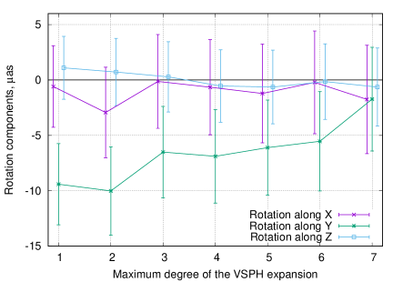
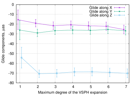
Figure 3: Rotation and glide components resulting from the VSPH expansion of the U16A - ICRF2 offsets. The values are slightly shifted along the horizontal for better readability.

Where do the U16A-ICRF2 systematic differences seen in figure 2 come from? A definitive answer is unclear at this point, but as shown by Ma et al. (2016), similar systematic differences have been linked to observations from stations belonging to the AUST network, which started observing in 2010. The authors showed that removing the observations from the AUST stations - as well as those from the KATH12M or HOBART12 stations - reduced some of those systematic differences. A systematic error in ICRF2 still cannot be ruled out.

4 Comparison of the VLBI positions with the Gaia Auxiliary Quasar Solution

Can a comparison with the Gaia positions help in identifying which solution is causing the offsets shown in the last section? In this section we compare the U16A and ICRF2 lists to the Gaia auxiliary quasar solution (Mignard et al., 2016) (hereafter called Gaia AQS). In opposition to the Gaia DR1 main catalog, the positions of the quasars in Gaia AQS were computed with the assumption that their proper motions were negligible. The median of the position differences between the two Gaia catalogs is 0.76 mas.

Before investigating the offsets between the catalogs, we can look at the distribution of the Gaia counterparts in RA and Dec. We refer to Mignard et al. (2016) for the problem of the selection of the optical counterparts of the ICRF2 objects in Gaia. Gaia AQS contains 2191 ICRF2 objects (64% of the ICRF2). We matched U16A with the Gaia DR1 main catalog with the same criteria as Mignard et al. (2016), and partitioned the sky with Healpix (Górski et al., 2005) into pixels of size 53.7 deg² (corresponding to Healpix’s Nside = 8). We then computed the ratio (number of U16A sources with a Gaia counterpart) / (number of U16A sources) in each pixel. The result is shown in figure 4. Low values indicate the location where the Gaia counterparts are missing; these are mostly along the galactic plane.

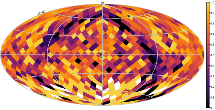
Figure 4: Equatorial map (Aitoff projection) showing the ratio (number of U16A sources with a Gaia DR1 counterpart) / (number of U16A sources) in pixels of $\sim$ 54 deg². Low (darker) values indicate a scarcity of Gaia counterparts. White pixels correspond to regions without data at this resolution.

Table 4 shows the median differences U16A-Gaia AQS and ICRF2-Gaia AQS. The latter comparison was investigated in detail by Mignard et al. (2016). We repeat some of their computations for the sake of exploring the improvement intrinsic to U16A. The formal errors of U16A and ICRF2 are displayed in table 7. For comparison, the median formal errors of Gaia AQS are 626 $\mu$as (in RA) and 564 $\mu$as (in Dec).

		262 defining		1289 VCS		640 Non-VCS		2191 sources
	RA*cos(Dec)	-104	(-277, 12)	-108	(-169, -27)	-171	(-254, -83)	-121	(-173, -76)
U16A-Gaia AQS	Dec	77	(11, 148)	-32	(-90, 30)	36	(-11, 91)	13	(-31, 48)
	Angular separation	584	(489, 652)	1009	(938, 1073)	897	(796, 991)	916	(865, 961)
	RA*cos(Dec)	-84	(-199, 10)	-4	(-109, 98)	-113	(-221, -39)	-62	(-124, 3)
ICRF2-Gaia AQS	Dec	135	(88, 236)	25	(-74, 86)	108	(30, 176)	69	(29, 111)
	Angular separation	601	(491, 666)	1346	(1325, 1551)	950	(818, 1034)	1159	(1097, 1225)

Table 4: Median differences in position in the sense U16A-Gaia AQS and ICRF2-Gaia AQS, in $\mu$as, with bootstrap BC_a confidence intervals with 95% coverage.

Overall, U16A is found to be significantly closer to Gaia AQS than ICRF2. This is mostly apparent for the VCS subset, where the offset has been reduced by $\sim$ 25 %, compared to just a few percents for the two other subsets. This demonstrates the improvement obtained by the re-observation of the VCS sources. As shown by the size covered by the confidence intervals, the overall scatter is also much reduced; the offset of the 2191 sources has MAD(U16A-Gaia) = 768 (724, 820) $\mu$as, while MAD(ICRF2-Gaia) = 1099 (1003, 1190) $\mu$as. This is despite a larger scatter in RA*cos(Dec) for the defining sources in U16A.

Table 5 shows the median differences between U16A and Gaia AQS limited to sources with $\geq$ 10 sessions. The positions of these sources are to be considered more precise. All the defining sources met this requirement, while only a few VCS sources did (we did not give any statistics for those). The larger scatter (i.e. the size of the bootstrap confidence interval) observed in RA*cos(Dec) is due to the defining sources, which now account for 262/657 $\sim$ 40% of this sample.

	262 defining		5 VCS	390 Non-VCS		657 sources
RA * cos(Dec)	-104	(-277, 12)	N.A.	-170	(-242, -63)	-141	(-219, -68)
Dec	77	(11, 148)	N.A.	39	(-11, 98)	52	(9, 92)
Absolute offset	584	(489, 652)	N.A.	703	(606, 814)	644	(589, 702)

Table 5: Median differences in position in the sense U16A-Gaia AQS, in $\mu$as, with bootstrap confidence intervals with 95% coverage. This concerns sources with $\geq$ 10 sessions. The statistics for the defining subset are identical to those in table 4, while the small number of VCS sources does not allow meaningful statistics.

4.1 Scatter depending on the declination

We investigated the systematic differences of U16A and ICRF2 with the declination, by computing the median slope of the angular separation with the Thiel-Sen method (Theil, 1950; Sen, 1968). We should expect to see a negative slope (i.e. larger offsets for Southern sources) due to the greater number of observing stations in the Northern Hemisphere, and the fact that Southern sources are typically observed from the Northern Hemisphere. This last feature results in small spatial sky coverage, which produces elongated uv-plane projections and highly elliptical beam patterns.

The results are listed in table 6 and shown in figure 5. The subsets have different results. The most important improvement brought by U16A concerns the VCS subset, which has the largest systematic difference in declination. The negative slope is significantly reduced by U16A, as well as its scatter. The defining subset has no statistically significant slope, both in U16A and ICRF2. The non-VCS subset does have a significant negative slope, very similar with U16A and ICRF2.

	262 Defining	1289 VCS	640 Non-VCS	2191 sources
Offset U16A - Gaia AQS	0.51 (-0.83, 1.90)	-3.00 (-4.44, -1.59)	-1.75 (-3.39, -0.29)	-1.49 (-2.40, -0.59)
Offset ICRF2 - Gaia AQS	0.29 (-1.09, 1.75)	-7.09 (-9.54, -4.75)	-1.87 (-3.51, -0.35)	-2.39 (-3.63, -1.19)

Table 6: The slope of the absolute offsets with declination, in $\mu$as.deg^-1. The slope and the 95% coverage confidence intervals (indicated between parentheses) are determined with the Thiel-Sen method.

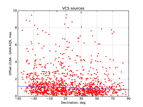
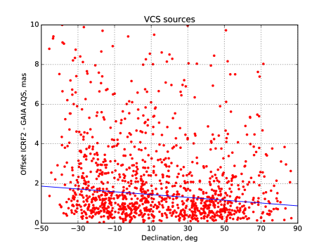
Figure 5: Absolute offsets of U16A and ICRF2 relative to Gaia AQS for the VCS subset, in mas. The Thiel-Sen line (see table 6) is also shown.

4.2 Consistency of the U16A formal errors

Since the U16A positions are improved compared to the ICRF2, the U16A formal errors should reflect this improvement and be smaller than their ICRF2 counterparts. We note that the ICRF2 formal errors were inflated (see Fey et al. (2015)), according to the formula

$$\sigma^{2}_{inflated}=(1.5\,\sigma)^{2}+(40\,\mu as)^{2}.$$ (1)

We show the distribution of the formal errors of U16A (inflated) and ICRF2 in figures 6 and 7. Approximately half of the U16A objects with inflated formal errors $<$ 0.1 mas are defining sources (and almost all the sources in the defining subset makes that cut), the other half corresponds to the 30% most precise non-VCS sources.

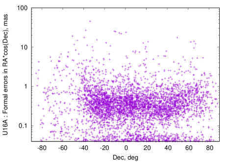
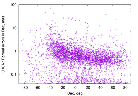
Figure 6: Formal errors of U16A, inflated following formula (1).

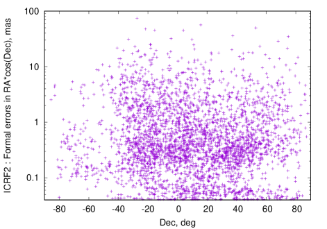
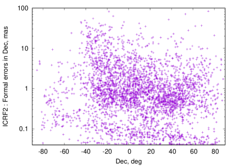
Figure 7: Formal errors of ICRF2.

Table 7 indicates some statistics of location and scale of the formal errors. The U16A median formal errors are smaller by $\sim$ 20-25% compared to ICRF2, while the scatter is reduced by $\sim$ 40-45%.

	Median	MAD
U16A $\sigma_{\alpha}^{*}$	323 (312, 332)	266 (256, 277)
U16A $\sigma_{\delta}$	548 (530, 561)	459 (439, 480)
ICRF2 $\sigma_{\alpha}^{*}$	397 (377, 416)	438 (413, 466)
ICRF2 $\sigma_{\delta}$	739 (705, 773)	832 (788, 874)

Table 7: Statistics of the formal errors of U16A (inflated) and ICRF2 in $\mu$as, with bootstrap confidence intervals with 95% coverage. The MAD represents the scatter of the formal errors around their median.

Note that the formal errors in declination are significantly larger than their counterparts in right ascension (both in ICRF2 and U16A). Because of the larger number of VLBI antennas in the Northern Hemisphere, there are many more (and longer) east-west VLBI baselines than there are north-south VLBI baselines. The larger number of observations on east-west baselines is thus reflected by the smaller uncertainties in right ascension.

We show the differences (U16A - Gaia AQS) normalized by their combined errors, i.e.,

$$\frac{(\alpha_{U}-\alpha_{G})\cos\delta}{(\sigma^{2}_{\alpha^{*}_{U}}+\sigma^{2}_{\alpha^{*}_{G}})^{1/2}}=\frac{\alpha_{U}-\alpha_{G}}{(\sigma^{2}_{\alpha_{U}}+\sigma^{2}_{\alpha_{G}})^{1/2}},\,\,\,\,\,\,\,\,\,\,\frac{\delta_{U}-\delta_{G}}{(\sigma^{2}_{\delta_{U}}+\sigma^{2}_{\delta_{G}})^{1/2}}$$ (2)

for both coordinates in figure 8.

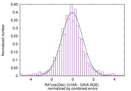
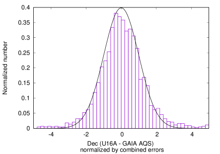
Figure 8: Normalized difference U16A - Gaia AQS. A normal distribution $\mathcal{N}(0,1)$ is shown for comparison.

Both distributions are similar to normal distributions, as expected. Estimations of the scale of the distributions are $\sigma$ = 1.071 (computed when limited to the interval [-3.5,3.5]), MAD = 1.026 for RA, and $\sigma$ = 1.114, MAD = 1.105 for Dec. The formal errors of U16A in figure 8 are not inflated. If they are inflated, we now have $\sigma$ = 1.022, MAD = 0.945 for RA, and $\sigma$ = 1.021, MAD = 0.978 for Dec. Though there are also a small number of large differences not accounted for by the formal errors, we conclude that they — in both U16A and Gaia AQS — broadly reflect the distribution of real errors for the majority of objects.

4.3 Global rotation and glide between the different frames

We applied the VSPH expansion to investigate the global rotation and glide between the U16A, Gaia AQS and ICRF2 frames. The results are shown in table 3.

Concerning the ICRF2-Gaia AQS offsets, our results are globally in agreement with the values found by Mignard et al. (2016). We attribute the differences in the rotation and glide components listed in their table 2 and shown in their figure 14 — which are within $\sim$ 20 $\mu$as from ours — to the different $l_{max}$, and to the sample selection, caused by different approaches for discarding outliers. In particular we recover the significant glide in the y and z-components between the ICRF2 and Gaia (which holds for all the $l_{max}$ considered). The significant 50 $\mu$as global rotation is a weaker result, supported only by $l_{max}=1,2$.

The statistically significant components of the U16A - Gaia AQS offsets are also weaker, in that they are not supported by all the $l_{max}$ considered in this study. If we accept that the 60-70 mas glides in the y and z-components are significant, they are notably smaller than their counterparts in the ICRF2 - Gaia AQS comparison, which corroborate the results found earlier in this paper.

5 Comparison of the new sources in U16A with Gaia DR1

In this section we turn our attention to the subset of 718 new sources included in U16A. These have not been previously compared to the Gaia positions. See table 1 for more details on these sources. We crossmatched the positions of the new U16A sources with the Gaia DR1 main catalog with a 1 arcsec radius, and obtained 425 unique matches (59% of the new U16A sources subset). The G magnitude distribution of these new sources is shown in figure 9 and is similar to, although somewhat fainter than, the rest of the sources.

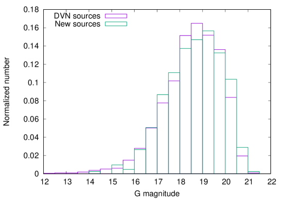
Figure 9: Distribution of the Gaia G magnitude of the DVN sources (defining, VCS and non-VCS) and the new U16A sources matched with Gaia DR1.

In order to compare the U16A - Gaia DR1 position differences with their formal errors, we computed the separation and the normalized separation $X$, as in Mignard et al. (2016), taking into account the correlation between right ascension and declination in both U16A and Gaia DR1. They are shown in figure 10. Since the errors are normally distributed, $X$ should have a Rayleigh distribution. In that case, the statistically expected number of sources with $X>3.67$ in a sample of size 425 is less than 0.5. We find 43 sources (10% of the sample) larger than this value. If we inflate the U16A errors, we now obtain 20 outliers (5% of the sample). This is similar to the results of Mignard et al. (2016) with regards to the position differences between ICRF2 and Gaia AQS. Half of the outliers have offsets larger than 150 mas.

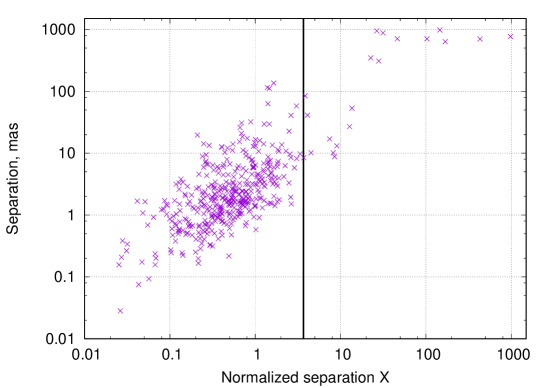
Figure 10: Separation U16A-Gaia DR1 versus the normalized separation $X$ for the new sources. The U16A errors have been inflated (see text). The vertical solid line demarcates the 3.67 statistically significant normalized separation X, thus, all sources to the right of this line are considered outliers.

5.1 PanSTARRS images

The sources presenting large position differences between ICRF2 and Gaia DR1 were recently investigated in detail by Makarov et al. (2017) using PanSTARRS images. Those large radio-optical differences can frequently be explained by the presence of close companions and extended structures, although a number of sources defy those explanations.

We looked at the PanSTARRS images of all the new 20 sources with normalized separation $>$ 3.67. The results are shown in table 8 in Appendix B, while figure 11 displays three sources representative of the classification in table 8: pair, extended, and no discernible feature. Of the 18 sources present in the PanSTARRS 3pi survey, about two thirds of them show distinctive features helping to explain the large offsets. These features are mostly the presence of a companion to the source (either true companion or chance alignement with a field star) and extended objects. Both features displace the optical photocenter detected by Gaia.

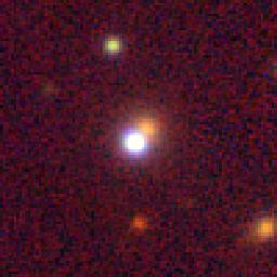
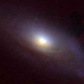
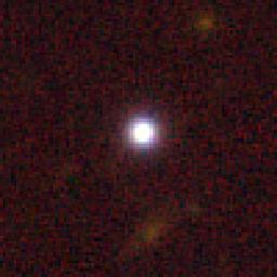
Figure 11: PanSTARRS images of some of the objects in table 8. Left: IVS 1750+093, offset = 948 mas. Middle: NGC 5635, offset = 27 mas. Right: IVS 1117-248, offset = 309 mas. The images are 25 arcsec (left and right) and 60 arcsec wide (middle) and are centered on the U16A radio positions.

6 Conclusions

We compared the current USNO ICRF solution (U16A) to the ICRF2 and Gaia catalogs. The U16A solution shows some significant differences of size 0.1 mas, and smaller, relative to ICRF2, although no significant global rotation is found between these two frames. While the first Gaia release does not have the precision necessary to resolve these systematic differences in detail, the U16A solution is found to be significantly closer to Gaia than ICRF2 in both coordinates. As mentioned above, those systematic differences in declination observed in the Southern Hemisphere might be caused by observations from some of the VLBI AUST stations since 2010. However, these affect mainly the positions of Southern sources. Since the improvement of the U16A is mostly due to the greater accuracy of its VCS subset — which is the largest component of the catalog, and is disproportionally distributed in the Northern Hemisphere and thus less influenced by the systematic differences — it is not surprising that U16A is still found to be globally more accurate than ICRF2. Finally, with the help of PanSTARRS images, we investigated the large radio-optical offsets that some of the new U16A sources display and found an explanation for two-thirds of them.

We thank the reviewer for providing comments that improved the quality of the paper. This work also benefited from discussions and comments from Christopher Dieck, Christopher S. Jacobs, and Norbert Zacharias. This work has made use of data from the European Space Agency (ESA) mission Gaia (http://www.cosmos.esa.int/gaia), processed by the Gaia Data Processing and Analysis Consortium (DPAC, http://www.cosmos.esa.int/web/gaia/dpac/consortium). Funding for the DPAC has been provided by national institutions, in particular the institutions participating in the Gaia Multilateral Agreement. The Pan-STARRS1 Surveys (PS1) have been made possible through contributions of the Institute for Astronomy, the University of Hawaii, the Pan-STARRS Project Office, the Max-Planck Society and its participating institutes, the Max Planck Institute for Astronomy, Heidelberg and the Max Planck Institute for Extraterrestrial Physics, Garching, The Johns Hopkins University, Durham University, the University of Edinburgh, Queen’s University Belfast, the Harvard-Smithsonian Center for Astrophysics, the Las Cumbres Observatory Global Telescope Network Incorporated, the National Central University of Taiwan, the Space Telescope Science Institute, the National Aeronautics and Space Administration under Grant No. NNX08AR22G issued through the Planetary Science Division of the NASA Science Mission Directorate, the National Science Foundation under grant No. AST-1238877, the University of Maryland, and Eötvös Loránd University (ELTE), and the Los Alamos National Laboratory. We made use of the Department of Defense Celestial Database of the USNO Astrometry Department. This research has made use of the VizieR catalog access tool, CDS, Strasbourg, France. The original description of the VizieR service was published in A&AS, 143, 23.

Appendix A Robust non-parametric regression

The mean curves in figure 2 were obtained by computing the robust equivalent of the Nadaraya-Watson estimator (Härdle & Tsybakov, 1988; Hall & Jones, 1990). The classic (non-robust) Nadaraya-Watson estimator (Nadaraya, 1964; Watson, 1964; Takezawa, 2005) is a local weighted constant defined by

$$\hat{m}(x)=\frac{\sum_{i=1}^{N}K(\frac{x-x_{i}}{h})Y_{i}}{\sum_{i=1}^{N}K(\frac{x-x_{i}}{h})}\,,$$ (A1)

where $x$ and $Y$ are the explanatory and dependent variables, respectively, and $K(u)$ is an appropriate smoothing kernel (here we used a Gaussian distribution). This estimator is the solution of the least squares problem

$$\operatorname*{minimize}_{m(x)}=\sum_{i=1}K\bigg{(}\frac{x-x_{i}}{h}\bigg{)}(Y_{i}-m(x))^{2}\text{ \hskip 14.22636pt or, equivalently, \hskip 14.22636pt}\sum_{i=1}K\bigg{(}\frac{x-x_{i}}{h}\bigg{)}(Y_{i}-m(x))=0\,.$$ (A2)

The bandwidth $h$ is a free parameter and determines whether the procedure overfits or underfits the real offsets.

A robust M-estimator (Huber & Ronchetti, 2009) for $m(x)$ is obtained by replacing the square with a robust function $\psi(u)$ and solving

$$\sum_{i=1}K\bigg{(}\frac{x-x_{i}}{h}\bigg{)}\psi\bigg{(}\frac{Y_{i}-m(x)}{s}\bigg{)}=0\,,$$ (A3)

where $s$ is a robust scale estimate. We used the Huber function

$$\begin{split}\psi(u)&=-1\text{\hskip 2.84544pt,\hskip 28.45274pt}u\leq-c\\ \psi(u)&=\frac{u}{c}\text{\hskip 2.84544pt,\hskip 28.45274pt}\,\,-c<u\leq c\\ \psi(u)&=1\text{\hskip 2.84544pt,\hskip 28.45274pt}\,\,\,\,u>c\end{split}$$ (A4)

where the coefficient $c=1.345$ is chosen so as to give a 95% efficiency in case the errors follow a simple Gaussian distribution (Holland & Welsh, 1977).

The estimate $\hat{m}(x)$ is obtained as follows:

1. Compute a local scale $s$, by computing the MAD of the $Y_{i}$ values in an interval around $x$ (say 10 degrees)

2. Solve iteratively for $m(x)$ with Newton’s method until a satisfactory convergence is reached

   $$m(x)^{(p+1)}=m(x)^{(p)}+\frac{\sum_{i=1}^{N}K(\frac{x-x_{i}}{h})\psi(\frac{Y_{i}-m(x)^{(p)}}{s})}{\sum_{i=1}^{N}K(\frac{x-x_{i}}{h})\psi^{\prime}(\frac{Y_{i}-m(x)^{(p)}}{s})}\,s\,,$$ (A5)

   where the initial guess $m(x)^{(0)}$ is the local median of the $Y_{i}$ values.

The choice of the bandwidth $h$ is crucial and is usually computed by using cross-validation, i.e. by finding $h$ that minimizes

$$CV(h)=\sum_{i=1}^{N}|Y_{i}-\hat{m}(x)^{(-i)}|\,,$$ (A6)

where $\hat{m}(x)^{(-i)}$ is the estimate computed by omitting the i^th source. Here the cross-validation step is robustified by using a sum of absolute values instead of the usual sum of squares (Leung, 2005).

The curves corresponding to the confidence intervals in figure 2 were computed using wild bootstrap resampling (Liu, 1988; Mammen, 1993). The non-parametric regression curve, computed as described above, gives the residuals $r_{i}=Y_{i}-\hat{m}(x_{i})$. The $Y_{i}$ values of the wild bootstrap samples are called $Y^{*}_{i}$ and are computed following

$$Y^{*}_{i}=Y_{i}+\varepsilon_{i}\,r_{i}\,,$$ (A7)

where the $\varepsilon_{i}$ follow a Rademacher distribution (see Flachaire (2005))

$$\begin{split}\varepsilon_{i}&=-1\text{\hskip 2.84544pt,\hskip 28.45274pt}p=0.5\\ \varepsilon_{i}&=1\text{\hskip 2.84544pt,\hskip 28.45274pt}\,\,\,\,p=0.5\,.\end{split}$$ (A8)

This amounts to randomly changing the sign of the residuals with respect to the mean curve.

A number of wild bootstrap samples (200) were computed for each mean curve, and the estimator $\hat{m}(x)$ was computed for each of the samples. The distribution of the resulting estimators $\hat{m}^{*}_{B}(x)$ with $B=1,...,200$ is then used to compute a 95 % confidence interval at each point $x_{i}$.

Appendix B U16A new sources with statistically significant radio-optical offsets with Gaia DR1

IVS name	Gaia DR1 source id	U16A RA	U16A Dec	U16A-Gaia	Features in PS1 image,	Gaia DR1	Gaia DR1 (mean / max			Number of
				offset	close Gaia neighbors and notes	excess noise	of excess noise / # of			VLBI
						(excess noise $\sigma$)	neighbors) within 0.1 deg			sessions
		deg	deg	mas		mas	mas	mas
Reasonable or tentative explanation
2048$+$370	1870909710012536832	312.711411916	37.2425211822	982.598	Possibly double sep. 1.5”, object at 5”	0. (0.)	1.305	7.769	81	2
1750$+$093	4488716878495401600	268.259853834	9.3333374835	947.725	Double sep. 1.5”	0.757 (3.88)	1.572	4.985	25	1
1740$-$169	4123749111948788480	265.775909615	-16.9711020499	772.631	Extended, Gaia neighbor at 4”	0.563 (1.93)	1.351	18.129	329	2
1858$-$212	4081909331557329664	285.268558136	-21.2003238993	708.536	Double sep. 0.5” or lens, Gaia neighbor at 4.9”	2.276 (1.92)	1.233	5.650	116	2
1701$-$246	4112708198449948160	256.25534233	-24.7527101571	706.490	2MASSX galaxy, Gaia neighbor at 4.7”	2.072 (13.53)	1.450	11.605	175	2
0931$+$103	589443338929476864	143.44211412	10.1524506152	84.398	NGC 2911, well-resolved galaxy with dust	15.667 (2370.78)	1.149	1.580	2	2
1151$+$126	3919707688292070784	178.543363944	12.4193758601	53.367	Galaxy	15.451 (278.46)	1.897	1.897	1	1
0310$+$410	239542077129105152	48.4901913843	41.2566596249	41.217	2MASSX galaxy	10.932 (1120.03)	1.175	3.194	17	1
NGC 5635	1280540719731180544	217.132340338	27.408953535	26.889	Well-resolved galaxy with dust	9.511 (2032.17)	1.992	1.992	1	2
2338$-$295	2327748343150961408	355.374009923	-29.320843913	10.171	Galaxy, Gaia neighbor at 3.8”	6.893 (381.44)	7.577	18.464	6	3
1638$+$118	4447290166579343616	250.245385766	11.734503378	10.124	Galaxy	3.147 (125.71)	1.270	2.414	7	2
1400$+$162	1231616197506959104	210.685473087	15.9990737579	8.458	Galaxy	1.260 (4.32)	2.280	2.779	3	2
No explanation
1834$-$155	4102987622313209472	279.406967906	-15.5455694377	880.142	Gaia neighbors at 1.7” and 3.7”	0.695 (8.67)	1.445	8.119	264	2
1911$+$013	4264732100629035264	288.560639404	1.40730671431	701.242		1.784 (20.78)	1.775	18.095	238	2
1143$+$052	3896995007877942016	176.632255657	4.97202463292	636.309		2.254 (1.09)	1.457	1.614	2	2
1117$-$248	3534310892614244992	170.038022714	-25.1354989919	308.826		0.626 (8.60)	0.938	1.719	7	5
1221$+$484	1545500550756588032	185.992627829	48.2160179775	13.151		4.171 (15.66)	1.006	1.258	3	1
1216$+$179	3946753131714484992	184.69418527	17.638130057	8.800		0.479 (2.52)			0	1
Sources not in PS1 images
1738$-$336	4053875702081678080	265.515372964	-33.6928928969	347.617	Gaia neighbor at 4.7”	1.159 (2.21)	1.361	5.386	369	2
0912$-$330	5630916907781932928	138.653004231	-33.2478928246	17.001		0. (0.)	0.838	4.475	23	1

Table 8: Features observed on the PanSTARRS images for the 20 sources with large separations U16A - Gaia DR1.

References

- Assafin et al. (2013) Assafin, M., Vieira-Martins, R, Andrei, A.H., Camargo, J.I.B., & da Silva Neto, D.N., 2013, MNRAS, 430, 2797
- Beasley et al. (2002) Beasley, A.J., Gordon, D., Peck, A.B., Petrov, L., MacMillan, D.S., Fomalont, E.E., & Ma, C. 2002, ApJS, 141, 13
- Berghea et al. (2016) Berghea, C.T, Makarov, V.V., Frouard, J., et al., 2016, The Astronomical Journal, 152, 53
- Chambers et al. (2016) Chambers, K.C., Magnier, E.A., Metcalfe, N. et al., 2016, The Pan-STARRS1 Surveys, arXiv:1612.05560
- DiCiccio & Efron (1996) DiCiccio, T. J., & Efron, B. 1996, Statistical Science, 11, 3, 189-228
- Efron & Tibshirani (1994) Efron, B., & Tibshirani, R. J. 1994, An introduction to the bootstrap, CRC press
- Fey et al. (2015) Fey, A. L., Gordon, D., Jacobs, C. S., et al. 2015, The Astronomical Journal, 150, 58
- Flachaire (2005) Flachaire, E. 2005, Computational Statistics & Data Analysis, 49, 361-376
- Gordon et al. (2016) Gordon, D., Jacobs, C., Beasley, A., Peck, A., Gaume, R., Charlot, P., Fey, A., Ma, C., Titov, O., & Boboltz, D., 2016, The Astronomical Journal, 151, 154
- Górski et al. (2005) Górski, K. M., Hivon, E., Banday, A. J., Wandelt, B. D., Hansen, F. K., Reinecke, M., & Bartelmann, M. 2005, The Astrophysical Journal, 622, 759-771
- Hall & Jones (1990) Hall P., & Jones, M.C. 1990, The annals of statistics, 18, 4, 1712
- Härdle & Tsybakov (1988) Härdle, W., & Tsybakov, A.B. 1988, The annals of statistics, 16, 1, 120
- Holland & Welsh (1977) Holland P.W., & Welsh, R.E. 1977, Communications in Statistics-Theory and Methods, 6, 9
- Huber & Ronchetti (2009) Huber, P.J., & Ronchetti, E.M. 2009, Robust Statistics, 2nd Edition, ISBN: 978-0-470-12990-6
- Jacobs et al. (2017) Jacobs, C.S, Bertarini, A., De Witt, A., Garcia-Miro, C., Gordon, D., Horiuchi, S., Lovell, J., McCallum, J., Mercolino, M., Quick, J., Snedeker, L., Bourda, G., & Charlot, P., ‘Tying multiple Radio Wavelength Celestial Frames to the Gaia Optical Frame’, IAU 330, Astrometry and Astrophysics in the Gaia Sky, Nice France, 24-28 April 2017
- Kovalev et al. (2017) Kovalev, Y.Y. , Petrov, L., & Plavin, A.V. 2017, A&A, 598, L1
- Leung (2005) Leung, D. H-Y. 2005, The annals of statistics, 33, 5, 2291
- Lindegren et al. (2016) Lindegren, L., Lammers, U., Bastian, U., et al. 2016, Astronomy & Astrophysics, 595, A4
- Liu (1988) Liu, R.Y. 1988, The annals of statistics, 16, 4, 1696-1708
- Ma et al. (1986) Ma, C., Clark, T.A., Ryan, J.W., Herring, T.A., Shapiro, I.I., Corey, B.E., Hinteregger, H.F., Rogers, A.E.E., Whitney, A.R., & Knight, C.A. 1986, AJ, 92, 1020
- Ma et al. (2016) Ma, C., MacMillan, D., Le Bail, K., & Gordon, D, 2016, ”Aspects of ICRF-3”, in International VLBI Service for Geodesy and Astrometry 2016 General Meeting Proceedings: “New Horizons with VGOS”, Eds. Dirk Behrend, Karen D. Baver, Kyla L. Armstrong, NASA/CP-2016-219016, p. 270-274
- Makarov & Murphy (2007) Makarov, V.V., & Murphy, D.W. 2007, AJ, 134, 1, 367-375
- Makarov et al. (2017) Makarov, V.V., Frouard, J., Berghea, C.T., Rest, A., Chambers, K.C., Kaiser, N., Kudritzki, R-P., & Magnier, E.A. 2017, The Astrophysical Journal Letters, 835, L30
- Mammen (1993) Mammen, E. 1993, The annals of statistics, 21, 1, 255-285
- Mignard & Klioner (2012) Mignard, F., & Klioner, S. 2012, Astronomy & Astrophysics, 547, A59
- Mignard et al. (2016) Mignard, F., Klioner, S., Lindegren, L., et al. 2016, Astronomy & Astrophysics, 595, A5
- Nadaraya (1964) Nadaraya, E. 1964, Theory Probab. Appl. 9, 141-142
- Orosz & Frey (2013) Orosz, G., & Frey, S. 2017, A&A, 553, A13
- Petrov & Kovalev (2017a) Petrov, L., & Kovalev, Y.Y. 2017, MNRAS, 467, 1, L71
- Schwarz (1978) Schwarz, G. 1978, The annals of statistics, 6, 2, 461-464
- Sen (1968) Sen, P.K. 1968, Journal of the American Statistical Association, 63, 324, 1379-1389
- Takezawa (2005) Takezawa, K. 2005, Introduction to Nonparametric regression, Wiley, ISBN 978-0-471-74583-9
- Theil (1950) Theil, H. 1950, Proceedings of the Royal Netherlands Academy of Sciences, 53, 386-392
- Watson (1964) Watson, G. 1964, Sankhyā Ser. 26, 359-372
- Zacharias & Zacharias (2014) Zacharias, N. & Zacharias, M.I. 2014, The Astronomical Journal, 147, 95