Constraint-Based Inference in Probabilistic Logic Programs

Abstract

Probabilistic Logic Programs (PLPs) generalize traditional logic programs and allow the encoding of models combining logical structure and uncertainty. In PLP, inference is performed by summarizing the possible worlds which entail the query in a suitable data structure, and using it to compute the answer probability. Systems such as ProbLog, PITA, etc., use propositional data structures like explanation graphs, BDDs, SDDs, etc., to represent the possible worlds. While this approach saves inference time due to substructure sharing, there are a number of problems where a more compact data structure is possible. We propose a data structure called Ordered Symbolic Derivation Diagram (OSDD) which captures the possible worlds by means of constraint formulas. We describe a program transformation technique to construct OSDDs via query evaluation, and give procedures to perform exact and approximate inference over OSDDs. Our approach has two key properties. Firstly, the exact inference procedure is a generalization of traditional inference, and results in speedup over the latter in certain settings. Secondly, the approximate technique is a generalization of likelihood weighting in Bayesian Networks, and allows us to perform sampling-based inference with lower rejection rate and variance. We evaluate the effectiveness of the proposed techniques through experiments on several problems. This paper is under consideration for acceptance in TPLP.

1 Introduction

A wide variety of models that combine logical and statistical knowledge can be expressed succinctly in the Probabilistic Logic Programming (PLP) paradigm. The expressive power of PLP goes beyond that of traditional probabilistic graphical models (eg. Bayesian Networks (BNs) and Markov Networks (MNs)) as can be seen in the examples in Figs. 1 and 2. These examples are written in PRISM, a pioneering PLP language [Sato and Kameya, 1997]. While the example in Fig. 1 encodes the probability distribution of a palindrome having a specific number of occurrences of a given character, the example in Fig. 2 encodes the probability that at least two persons in a given set have the same birthday. Examples such as these and other models like reachability over graphs with probabilistic links illustrate how logical clauses can be used to specify models that go beyond what is possible in traditional probabilistic graphical models.

⬇

% Generate a list of N random variables.

genlist(0, []).

genlist(N, L) :-

N > 0,

msw(flip, N, X),

L = [X|L1],

N1 is N-1,

genlist(N1, L1).

% Evidence: list is a palindrome.

evidence(N) :-

genlist(N, L), palindrome(L).

% Query: string has K ’a’s

query(N, K) :-

genlist(N, L), count_as(L, K).

⬇

% Check if a given list is a palindrome

palindrome(L) :- phrase(palindrome, L).

palindrome --> [].

palindrome --> [_X].

palindrome --> [X], palindrome, [X].

% Query condition:

count_as([], 0).

count_as([X|Xs], K) :-

count_as(Xs, L),

(X=a -> K is L+1; K=L).

% Domains:

values(flip, [a,b]).

% Distribution parameters:

set_sw(flip, [0.5, 0.5]).

Figure 1: Palindrome PLP

The Driving Problem.

The expressiveness of PLP comes at a cost. Since PLP is an extension to traditional logic programming, inference in PLP is undecidable in general. Inference is intractable even under strong finiteness assumptions. For instance, consider the PRISM program in Fig. 1. In that program, genlist/2 defines a list of the outcomes of $N$ identically distributed random variables ranging over {a,b} (through msw/3 predicates). Predicate palindrome/1 tests, using a definite clause grammar definition, if a given list is a palindrome; and count_as/2 tests if a given list contains $k$ (not necessarily consecutive) “a”s. Using these predicates, consider the inference of the conditional probability of $\mathtt{query}(n,k)$ given $\mathtt{evidence}(n)$: i.e., the probability that an $n$-element palindrome has $k$ “a”s.

⬇

% Two from a population of

% size N share a birthday.

same_birthday(N) :-

person(N, P1),

msw(b, P1, D),

person(N, P2),

P1 < P2,

msw(b, P2, D)

% Bind P, backtracking

% through 1..N

person(N, P) :-

basics:for(P, 1, N).

% Distribution parameters:

:- set_sw(b(_),

uniform(1,365)).

Figure 2: Birthday PLP

The conditional probability is well-defined according to PRISM’s distribution semantics [Sato and Kameya, 2001]. However, PRISM itself will be unable to correctly compute the conditional query’s probability, since the conditional query, as encoded above, will violate the PRISM system’s assumptions of independence among random variables used in an explanation. Moreover, while the probability of goal evidence(N) can be computed in linear time (using explanation graphs), the conditional query itself is intractable, since the computation is dominated by the binomial coefficient $\binom{N}{k}$. This is not surprising since probabilistic inference is intractable over even simple statistical models such as Bayesian networks. Consequently, exact inference techniques used in PLP systems such as PRISM, ProbLog [De Raedt et al., 2007] and PITA [Riguzzi and Swift, 2011], have exponential time complexity when used on such programs.

Approximate inference based on rejection sampling also performs poorly, rejecting a vast number of generated samples, since the likelihood of a string being a palindrome decreases exponentially in $N$. Alternatives such as Metropolis-Hastings-based Markov Chain Monte Carlo (MCMC) techniques [Hastings, 1970, e.g.] do not behave much better: the chains exhibit poor convergence (mixing), since most transitions lead to strings inconsistent with evidence. Gibbs-sampling-based MCMC [Geman and Geman, 1984] cannot be readily applied since the dependencies between random variables are hidden in the program and not explicit in the model.

Our Approach.

In this paper, we use PRISM’s syntax and distribution semantics, but without the requirements imposed by the PRISM system, namely, that distinct explanations of an answer are pairwise mutually exclusive and all random variables within an explanation are independent. We, however, retain the assumption that distinct random variable instances are independent. Thus we consider PRISM programs with their intended model-theoretic semantics, rather than that computed by the PRISM system.

We propose a data structure called Ordered Symbolic Derivation Diagram (OSDD) which represents the set of possible explanations for a goal symbolically. The key characteristic of OSDDs is the use of constraints on random variables. This data structure is constructed through tabled evaluation on a transformed input program. For example, the OSDD for “same_birthday(3)” from example Fig. 2 is shown in Fig. 3(b). This data structure can be used for performing exact inference in polynomial time as will be described later. In cases where exact inference is intractable, OSDDs can be used to perform sampling based inference. For example, the OSDD for “evidence(6)” from example Fig. 1 is shown in Fig. 3 (a) and can be used for performing likelihood weighted sampling [Fung and Chang, 1990; Shachter and Peot, 1990].

(a) OSDD for evidence(6)		(b) OSDD for same_birthday(3)

Figure 3: OSDDs for introductory examples

The rest of the paper is organized as follows. In Section 2 we formally define OSDDs and the operations on OSDDs. Next we give the procedure for construction of OSDDs. This procedure relies on a program transformation which is explained in Section 3. Next we give the exact and approximate inference algorithms using OSDDs in Section 4. We present the experimental results in Section 5, related work in Section 6, and concluding remarks in Section 7.

2 Ordered Symbolic Derivation Diagrams

Notation:

We assume familiarity with common logic programming terminology such as variables, terms, substitutions, predicates and clauses. We use Prolog’s convention, using identifiers beginning with a lower case letter to denote atomic constants or function symbols, and those beginning with an upper case letter to denote variables. We often use specific symbols such as $t$ to denote ground terms, and $i,j,k$ to denote integer indices. We assume an arbitrary but fixed ordering ”$\prec$” among variables and ground terms.

A type is a finite collection of ground terms. In this paper, types represent the space of outcomes of switches or random processes. For example in Palindrome example of Fig 1, the set of values $\{a,b\}$ is a type. A variable $Y$ referring to the outcome of a switch is a typed variable; its type, denoted $type(Y)$, is deemed to be the same as the space of outcomes of $s$. The type of a ground term $t$ can be any of the sets it is an element of.

Definition 1 (Atomic Constraint).

An atomic constraint, denoted $\beta$, is of the form $\{X=T\}$ or $\{X\neq T\}$, where $X$ is a variable and $T$ is a variable or a ground term of the same type as $X$. When $T$ is a ground term, we can assert that $type(T)=type(X)$.

A set of atomic constraints representing their conjunction is called a constraint formula. Constraint formulas are denoted by symbols $\gamma$ and $\phi$. Note that atomic constraints are closed under negation, while constraint formulas are not closed under negation.

Definition 2 (Constraint Graph).

The constraint graph for a constraint formula $\gamma$ is labeled undirected graph, whose nodes are variables and ground terms in $\gamma$. Edges are labeled with ”$=$” and ”$\not=$” such that

• $T_{1}$ and $T_{2}$ are connected by an edge labeled ”$=$” if, and only if, $T_{1}=T_{2}$ is entailed by $\gamma$.

• $T_{1}$ and $T_{2}$ are connected by an edge labeled ”$\not=$” if, and only if, $T_{1}\not=T_{2}$ is entailed by $\gamma$, and at least one of $T_{1},T_{2}$ is a variable.

Note that a constraint graph may have edges between two terms even when there is no explicit constraint on the two terms in $\gamma$.

Definition 3 (Ordering).

Based on an (arbitrary but fixed) ordering among ground terms, we define an ordering on ground switch instance pairs $(s,i)$ and $(s^{\prime},i^{\prime})$ as follows:

• If $i\prec i^{\prime}$ then $(s,i)\prec(s^{\prime},i^{\prime})$ for all ground terms $s$ and $s^{\prime}$.

• If $i=i^{\prime}\land s\prec s^{\prime}$ then $(s,i)\prec(s^{\prime},i^{\prime})$.

• If $i=i^{\prime}\land s=s^{\prime}$ then $(s,i)=(s^{\prime},i^{\prime})$.

Canonical representation of constraint formulas.

A constraint formula is represented by its constraint graph which in turn can be represented as a set of triples $(source,destination,constraint)$ each of which represents an edge in the constraint graph. Recall that variables and ground terms can be compared using total order $\prec$. Assuming an order between the two symbols ”$=$” and ”$\not=$”, we can define a lexicographic order over each edge triple, and consequently order the elements of the edge set. The sequence of edge triples following the above order is a canonical representation of a constraint formula. Using this representation, we can define a total order, called the canonical order, among constraint formulas themselves given by the lexicographic ordering defined over the edge sequences.

Given any constraint formula $\gamma=\{\beta_{1},\beta_{2},\ldots,\beta_{n}\}$, its negation $\neg\gamma$ is given by a set of constraint formulas $\neg\gamma=\{\{\neg\beta_{1}\},\{\beta_{1},\neg\beta_{2}\},\ldots,\{\beta_{1},\beta_{2},\ldots,\beta_{n-1},\neg\beta_{n}\}\}$. The above defines negation of a formula to be a set of constraint formulas which are pairwise mutually exclusive and together represent the negation.

The set of solutions of a constraint formula $\gamma$ is denoted $\mbox{$[\![$}\gamma\mbox{$]\!]$}$ and their projection onto a variable $X\in Vars(\gamma)$ is denoted $\mbox{$\mbox{$[\![$}\gamma\mbox{$]\!]$}$}_{X}$. The constraint formula is unsatisfiable if $\mbox{$\mbox{$[\![$}\gamma\mbox{$]\!]$}$}=\emptyset$, and satisfiable otherwise. Note that substitutions can also be viewed as constraint formulas.

PRISM.

The following is a high-level overview of PRISM. PRISM programs have Prolog-like syntax (see Fig. 4). In a PRISM program the msw relation (“multi-valued switch”) has a special meaning: msw(X,I,V) says that V is the outcome of the I-th instance from a family X of random processes. The set of variables $\{\mathtt{V}_{i}\mid\mathtt{msw(}p,i,\mathtt{V}_{i}\mathtt{)}\}$ are i.i.d. for a given random process $p$.

The distribution parameters of the random variables are specified separately.

The program in Fig. 4 encodes a Hidden Markov Model (HMM) in PRISM.

Figure 4: PRISM program for an HMM

The set of observations is encoded as facts of predicate obs, where obs(I,V) means that value V was observed at time I. In the figure, the clause defining hmm says that T is the N-th state if we traverse the HMM starting at an initial state S (itself the outcome of the random process init). In hmm_part(I, N, S, T), S is the I-th state, T is the N-th state. The first clause of hmm_part defines the conditions under which we go from the I-th state S to the I+1-th state NextS. Random processes trans(S) and emit(S) give the distributions of transitions and emissions, respectively, from state S.

The meaning of a PRISM program is given in terms of a distribution semantics [Sato and Kameya, 1997, 2001]. A PRISM program is treated as a non-probabilistic logic program over a set of probabilistic facts, the msw relation. An instance of the msw relation defines one choice of values of all random variables. A PRISM program is associated with a set of least models, one for each msw relation instance. A probability distribution is then defined over the set of models, based on the probability distribution of the msw relation instances. This distribution is the semantics of a PRISM program. Note that the distribution semantics is declarative. For a subclass of programs, PRISM has an efficient procedure for computing this semantics based on OLDT resolution [Tamaki and Sato, 1986].

Inference in PRISM proceeds as follows. When the goal selected at a step is of the form msw(X,I,Y), then Y is bound to a possible outcome of a random process X. Thus in PRISM, derivations are constructed by enumerating the possible outcomes of each random variable. The derivation step is associated with the probability of this outcome. If all random processes encountered in a derivation are independent, then the probability of the derivation is the product of probabilities of each step in the derivation. If a set of derivations are pairwise mutually exclusive, the probability of the set is the sum of probabilities of each derivation in the set. PRISM’s evaluation procedure is defined only when the independence and exclusiveness assumptions hold. Finally, the probability of an answer is the probability of the set of derivations of that answer.

OSDD.

We use OSDDs to materialize derivations in a compact manner. OSDDs share a number of features with Binary Decision Diagrams (BDDs) [Bryant, 1992] and Multivalued Decision Diagrams (MDDs) [Kam et al., 1998]. BDDs are directed acyclic graphs representing propositional boolean formulas, with leaves labeled from $\{0,1\}$ and internal nodes labeled with propositions. In a BDD, each node has two outgoing edges labeled $0$ and $1$, representing a true and false valuation, respectively, for the node’s proposition. An MDD generalizes a BDD where internal nodes are labeled with finite-domain variables, and the outgoing edges are labeled with the possible valuations of that variable. In an OSDD, internal nodes represent switches and the outgoing edges are labeled with constraints representing the possible outcomes of that node’s switch.

Definition 4 (Ordered Symbolic Derivation Diagram).

An ordered symbolic derivation diagram over a set of typed variables $V$ is a tree, where leaves are labeled from the set $\{0,1\}$ and internal nodes are labeled by triples of the form $(s,k,Y)$, where $s$ and $k$ are switch and instance respectively and $Y\in V$. We call $Y$ the output variable of the node. The edges are labeled by constraint formulas over $V$. We represent OSDDs by textual patterns $(s,k,Y)[\gamma_{i}:\psi_{i}]$ where $(s,k,Y)$ is the label of the root and each sub-OSDD $\psi_{i}$ is connected to the root by an edge labeled $\gamma_{i}$. OSDDs satisfy the following conditions:

1. Ordering: For internal nodes $n=(s,k,Y)$ and $n^{\prime}=(s^{\prime},k^{\prime},Y^{\prime})$, if $n$ is the parent of $n^{\prime}$, then $(s,k)\prec(s^{\prime},k^{\prime})$. The edges are ordered by using the canonical ordering of the constraint formulas labeling them.

2. Mutual Exclusion: The constraints labeling the outgoing edges from an internal node are pairwise mutually exclusive (i.e., for each $\gamma_{i}$ and $\gamma_{j}$, $\mbox{$\mbox{$[\![$}\gamma_{i}\land\gamma_{j}\mbox{$]\!]$}$}=\emptyset$).

3. Completeness: Let $(s,k,Y)[\gamma_{i}:\psi_{i}]$ be a sub-OSDD and let $\sigma$ be any substitution that satisfies all constraints on the path from root to the given sub-OSDD such that $\sigma(Y)\in\mbox{\it type\/}(Y)$. Then there is a $i$ such that $\sigma$ satisfies $\gamma_{i}$.

4. Urgency: Let $\mathcal{O}(n)$ be the set of output variables in the path from the root to node $n$ (including $n$). Then for every constraint formula $\gamma_{i}$ labeling an outgoing edge from $n$, it holds that $Vars(\gamma_{i})\subseteq\mathcal{O}(n)$ and for every ancestor $n^{\prime}$ of $n$, $Vars(\gamma_{i})\not\subseteq\mathcal{O}(n^{\prime})$.

5. Explicit constraints: If constraint formula $\gamma_{i}$ out of a node $n$ entails an implicit atomic constraint $\beta$ on variables in $\mathcal{O}(n)$, then $\beta$ occurs explicitly in the path from root to $n$. A consequence of this condition is that the conjunction of constraint formulas labeling edges in a path will be satisfiable.

A tree which satisfies all conditions of an OSDD except conditions 4 and 5 is called an improper OSDD.

Example 1 (OSDD properties).

We illustrate the definiton by using the OSDD shown in Fig. 3(b). The OSDD is represented by the textual pattern $(b,1,X1)[\emptyset:\psi_{1}]$ where $\psi_{1}$ is the sub-tree rooted at the node labeled $msw(b,2,X2)$, which in turn can be represented by the textual pattern $(b,2,X2)[\{X1=X2\}:1,\{X1\neq X2\}:\psi_{2}]$ where $\psi_{2}$ is the sub-tree rooted at the node $msw(b,3,X3)$ and so on. The internal nodes satisfy the total ordering based on the instance numbers. All outgoing edges from an internal node are pairwise mutually exclusive. For instance for the outgoing edges of the node labeled $msw(b,3,X3)$, $X1=X3$ is mutually exclusive w.r.t to $X1\neq X3,X2=X3$ and $X1\neq X3,X2\neq X3$. Similarly, $X1\neq X3,X2=X3$ is mutually exclusive to $X1\neq X3,X2\neq X3$. Consider the sub-OSDD rooted at $msw(b,2,X2)$ any substitution that grounds $X1,X2$ satisfies the (empty) constraints on the path from the root to that sub-tree. Further any such substitution will satisfy exactly one of the edge constraints $X1=X2$ or $X1\neq X2$. It is obvious from the example that urgency is satisfied. Finally consider the constraint formula $X1\neq X3,X2=X3$. This entails the implicit constraint $X1\neq X2$. However, this constraint is explicitly found in the path from the root to that sub-tree. Therefore the OSDD in Fig. 3(b) is a proper OSDD.

OSDDs can be viewed as representing a set of explanations or derivations where a node of the form $(s,k,Y)$ binds $Y$. This observation leads to the definition of bound and free variables:

Definition 5 (Bound and Free variables).

Given an OSDD $\psi=(s,k,Y)[\gamma_{i}:\psi_{i}]$ the bound variables of $\psi$, denoted $BV(\psi)$, are the output variables in $\psi$. The free variables of $\psi$, denoted $FV(\psi)$, are those variables which are not bound.

Each OSDD corresponds to an MDD which can be constructed as follows.

Definition 6 (Grounding).

Given an OSDD $\psi=(s,k,Y)[\gamma_{i}:\psi_{i}]$, the MDD corresponding to it is denoted $\mathcal{G}(\psi)$ and is recursively defined as $\mathcal{G}(\psi)=(s,k,Y)[\alpha_{j}:\mathcal{G}(\psi_{j}[\alpha_{j}/Y])]$ where $\alpha_{j}\in type(Y)$ and $\psi_{j}=\psi_{i}$ such that $\gamma_{i}[\alpha_{j}/Y]$ is satisfiable.

Example 2 (Grounding).

As an example consider a smaller version of the OSDD shown in Fig. 3(a) as shown in Fig. 5(a). In the first step of the grounding, all values satisfy the (empty) constraint of the outgoing edge. Therefore we get two subtrees which are identical except the substitution that is applied to the variable $X1$. In the next step (which we omit here), the subtrees get ground. Consider the left subtree, the value “a” satisfies the left branch, while the value “b” satisfies the right branch. Therefore in effect those edges get relabelled by “a” and “b” and similarly for the right subtree.

(a) OSDD		(b) Grounding

Figure 5: Example of grounding OSDD

Canonical OSDD representation.

Given a total order among variables and terms, the order of nodes in an OSDD is fixed. We can further order the outgoing edges uniquely based on the total order of constraints labeling them. This yields a canonical representation of OSDDs. In the rest of the paper we assume that OSDDs are in canonical form.

Definition 7 (Equivalence).

All OSDD leaves which have the same node label are equivalent. Two OSDDs $\psi=(s,k,Y)[\gamma_{i}:\psi_{i}]$ and $\psi^{\prime}=(s,k,Y^{\prime})[\gamma^{\prime}_{i}:\psi^{\prime}_{i}]$ are equivalent if $\forall i.\ \ [\gamma_{i}:\psi_{i}]=[\gamma^{\prime}_{i}:\psi^{\prime}_{i}][Y/Y^{\prime}]$.

We now define common operations over OSDDs which can create OSDDs from primitives.

Definition 8 (Conjunction/Disjunction).

Given OSDDs $\psi=(s,k,Y)[\gamma_{i}:\psi_{i}]$ and $\psi^{\prime}=(s^{\prime},k^{\prime},Y^{\prime})[\gamma^{\prime}_{j}:\psi^{\prime}_{j}]$, let $\oplus$ stand for either $\land$ or $\lor$ operation. Then $\psi\oplus\psi^{\prime}$ is defined as follows.

• If $(s,k)\prec(s^{\prime},k^{\prime})$, then $\psi\oplus\psi^{\prime}=(s,k,Y)[\gamma_{i}:\psi_{i}\oplus\psi^{\prime}]$

• If $(s^{\prime},k^{\prime})\prec(s,k)$ then $\psi\oplus\psi^{\prime}=(s^{\prime},k^{\prime},Y^{\prime})[\gamma^{\prime}_{j}:\psi^{\prime}_{j}\oplus\psi]$

• If $(s,k)=(s^{\prime},k^{\prime})$, first we apply the substitution $[Y/Y^{\prime}]$ to the second OSDD. Then $\psi\oplus\psi^{\prime}=(s,k,Y)[\gamma_{i}\land\gamma^{\prime}_{j}:\psi_{i}\oplus\psi^{\prime}_{j}]$.

Example 3 (Conjunction/Disjunction).

Consider the input OSDDs in Fig. 6(a). Their disjunction is shown in Fig. 6(b). Disjunction of this OSDD with a third OSDD involving switch instance pairs $(b,2),(b,3)$ results in the OSDD shown in Fig. 3(b).

(a) Input OSDDs		(b) Disjunction

Figure 6: Disjunction of OSDDs

Although OSDDs have been defined as trees, we can turn them into DAGs by combining equivalent subtrees. It is easy to generalize the above operations to work directly over DAGs. The above operation may produce improper OSDDs, but can be readily transformed to proper OSDDs as follows

Transformation from improper to proper OSDDs.

(a) Improper OSDD		(b) Proper OSDD

Figure 7: Transformation example

When performing and/or operations over proper OSDDs, the resulting OSDD may be improper. For instance, consider one OSDD with variables $X,Z$, and another with variables $Y,Z$. Constraints between $X$ and $Z$, and those between $Y$ and $Z$ may imply constraints between $X$ and $y$ that may not be explicitly present in the resulting OSDD, thereby violating the condition of explicit constraints (Def.  4).

Fig. 7(a) shows an improper OSDD that violates the explicit constraints condition. For example, the edge $(Z,\Psi_{1})$, leading to the sub-OSDD $\Psi_{1}$, has edge constraints which imply $X=Y$ while the edges leading to $\Psi_{2}$ and $\Psi_{3}$ imply $X\neq Y$.

An improper OSDD can be converted into a proper one by rewriting it using a sequence of steps as follows. First, we identify an implicit constraint and where it may be explicitly added without violating the urgency property. In the example, we identify $X=Y$ as implicit, and attempt to introduce it on the outgoing edges of node labeled $Y$. This introduction splits the edge from $Y$ to $Z$ into two: one labeled $X=Y$, and another labeled $X\neq Y$, the negation of the identified constraint. The original child rooted at $Z$ is now replicated due to this split. We process each child, eliminating edges and corresponding sub-OSDDs whenever the constraints are unsatisfiable. In the example in Fig. 7(b) we see that the edges $(Z,\Psi_{2})$ and $(Z,\Psi_{3})$ have been removed from $\Psi_{Z_{1}}$ since their constraint formula are inconsistent with $X=Y$. We repeat this procedure until no implicit constraints exist in $\Psi$.

Constraint application.

An OSDD may be specialized for a context which constrains its variables, as follows.

Definition 9 (Constraint application).

Given an OSDD $\psi=(s,k,Y)[\gamma_{i}:\psi_{i}]$ and an atomic constraint $\beta$, the application of $\beta$ to $\psi$ results in a new OSDD $\psi^{\prime}$ as follows:

• Application of $\beta$ to $0,1$ yields $0,1$ respectively.

• If $Vars(\beta)\subseteq\mathcal{O}(n)$ where $n$ is the root of $\psi$, then $\psi^{\prime}=(s,k,Y)[\gamma_{i}\land\beta:\psi_{i},\neg\beta:0]$

• Else $\psi^{\prime}=(s,k,Y)[\gamma_{i}:\psi^{\prime}_{i}]$ where each $\psi^{\prime}_{i}$ results from the application of $\beta$ to $\psi_{i}$.

Properties.

OSDDs and the operations defined above have a number of properties necessary for their use in representing explanations for query evaluation in PLPs.

Proposition 1 (Closure).

OSDDs are closed under conjunction and disjunction operations.

The following shows that conjunction and disjunction operations over OSDDs lift the meaning of these operations over ground MDDs.

Proposition 2 (Compatibility with Grounding).

Let $\psi=(s,k,Y)[\gamma_{i}:\psi_{i}]$ and $\psi^{\prime}=(s^{\prime},k^{\prime},Y^{\prime})[\gamma^{\prime}_{j}:\psi^{\prime}_{j}]$ be two OSDDs, then

$$\mathcal{G}(\psi\oplus\psi^{\prime})=\mathcal{G}(\psi)\oplus\mathcal{G}(\psi^{\prime}).$$

3 Construction

Given a definite PLP program and a ground query, we construct an OSDD as the first step of the inference process. The construction is done via constraint-based tabled evaluation over a transformed program. At a high level, each $n$-ary predicate $p/n$ in the original PLP program is transformed into a $n+2$-ary predicate $p/(n+2)$ with one of the new arguments representing an OSDD at the time of call to $p$, and the other representing OSDDs for answers to the call.

For simplicity, although the transformed program represents OSDDs as Prolog terms, we reuse the notation from Section 2 to describe the transformation.

Transformation.

We use $\overline{T_{1}},\overline{T_{2}},\ldots$ to represent tuples of arguments. Clauses in a definite program may be of one of two forms:

• Fact $p(\overline{T})$: is transformed to another fact of the form $p(\overline{T},\mathtt{O},\mathtt{O})$, denoting that a fact may bind its arguments but do not modify a given OSDD.

• Clause $\mbox{\it head\/}\leftarrow\mbox{\it body\/}$: without loss of generality, we assume that the body is binary: i.e., clauses are of the form $p(\overline{T})\leftarrow q(\overline{T_{1}}),r(\overline{T_{2}})$. Such clauses are transformed into $p(\overline{T},\mathtt{O_{1}},\mathtt{O_{3}})\leftarrow q(\overline{T_{1}},\mathtt{O_{1}},\mathtt{O_{2}}),r(\overline{T_{2}},\mathtt{O_{2}},\mathtt{O_{3}})$

For each user-defined predicate $p/n$ in the input program, we add the following directive for the transformed predicate $p/(n+2)$

:- table $p(\_,\ldots,\_,$ lattice(or/3)).

which invokes answer subsumption [Swift and Warren, 2010] to group all answers by their first $n+1$ arguments, and combine the $n+2$-nd argument in each group using or/3, which implements the disjunction operation over OSDDs.

Constraint-Based Evaluation.

An important aspect of OSDD construction is constraint processing. Our transformation assumes that constraints are associated with variables using their attributes [Holzbaur, 1992]. We assume the existence of the following two predicates:

• inspect(X, C), which, given a variable X, returns the constraint formula associated with X; and

• store(C), which, given a constraint formula C, annotates all variables in C with their respective atomic constraints.

For tabled evaluation, we assume that each table has a local constraint store [Sarna-Starosta and Ramakrishnan, 2007]. Such a constraint store can be implemented using the above two predicates.

OSDD Builtins.

The construction of the transformed program is completed by defining predicates to handle the two constructs that set PLPs apart:

• msw(S, K, X, $\mathtt{O_{1}}$, $\mathtt{O_{1}}$): Note that msw’s in the body of a clause would have been transformed to a 5-ary predicate. This predicate is defined as:

  $$msw(S,K,Y,\mathtt{O_{1}},\mathtt{O_{2}})\leftarrow \mathtt{inspect(}Y,\gamma\mathtt{)},$$

  $$(\gamma=\{\}\rightarrow O=(S,K,Y)[\{\}:1]$$

  $$;\ \ O=(S,K,Y)[\gamma:1,\neg\gamma:0]$$

  $$),\mathtt{and(O_{1},O,O_{2})}.$$

  where and/3 implements conjunction operation over OSDDs.

• Constraint handling: constraints in the input program will be processed using:

  $$constraint(C,\mathtt{O_{1}},\mathtt{O_{2}})\leftarrow ((\mbox{\it Vars\/}(C)\cap BV(\mathtt{O_{1}}))\not=\emptyset$$

  $$\rightarrow\mathtt{O_{2}}=\mathtt{applyConstraint}(C,\mathtt{O_{1}})$$

  $$;\ \ \mathtt{O_{2}}=\mathtt{O_{1}}$$

  $$),\mathtt{store}(C).$$

  where applyConstraint is an implementation of Defn. 9

To compute the OSDD for a ground atom $q(\overline{X})$ in the original program, we evaluate $q(\overline{X},1,O)$ to obtain the required OSDD as $O$.

4 Inference

Exact Inference.

Given an OSDD $\psi=(s,k,Y)[\gamma_{i}:\psi_{i}]$, let $Dom(FV(\psi))$ be the Cartesian product of the types of each $X\in FV(\psi)$. We define a function $\pi$ which maps an OSDD $\psi$ and a substitution $\sigma\in Dom(FV(\psi))$ to $\mathbb{R}$. Its definition for leaves is as follows

$$\pi(1,\emptyset)=1\text{ and }\pi(0,\emptyset)=0.$$

Next for an OSDD $\psi$ and an arbitrary substitution $\sigma^{\prime}$, define $\Pi(\psi,\sigma^{\prime})$ to be

$$\Pi(\psi,\sigma^{\prime})=\sum_{\sigma:\sigma\nparallel\sigma^{\prime}}\pi(\psi,\sigma),$$

where constraint formulas $\sigma$ and $\sigma^{\prime}$ are said to be compatible if their conjunction is satisfiable (denoted $\sigma\nparallel\sigma^{\prime}$). For internal nodes we define $\pi(\psi,\sigma)$ as

$$\pi(\psi,\sigma)=\sum_{i}\sum_{y\in\mbox{$\mbox{$[\![$}\gamma_{i}\sigma\mbox{$]\!]$}$}_{Y}}P(Y=y)\Pi(\psi_{i},\sigma[y/Y]).$$

where $P(Y=y)$ is the probability that $k$-th instance of $s$ has outcome $y$.

Given a ground query whose OSDD is $\psi$ we return the answer probability as $\Pi(\psi,\emptyset)$.

Proposition 3 (Complexity).

The time complexity of probability computation of OSDD $\psi$ is $O(D\cdot N\cdot exp(V))$ where $D$ is the maximum cardinality of all types, $N$ is the number of nodes in $\psi$, and $V$ is the size of the largest set of free variables among all internal nodes of $\psi$.

Under certain conditions we can avoid the exponential complexity of the naive probabilistic inference algorithm. By exploiting the regular structure of the solution space to a constraint formula we avoid the explicit summation $\sum_{y\in\mbox{$\mbox{$[\![$}\gamma_{i}\sigma\mbox{$]\!]$}$}_{Y}}$. In this case we say that $\gamma_{i}$ is measurable. We formally define measurability and a necessary and sufficient condition for measurability.

Definition 10 (Measurability).

A satisfiable constraint formula $\gamma$ is said to be measurable w.r.t $X\in Vars(\gamma)$ if for all ground substitutions $\sigma$ on $Vars(\gamma)\setminus\{X\}$ which satisfy $\gamma$, $|\mbox{$\mbox{$[\![$}\gamma\sigma\mbox{$]\!]$}$}_{X}|$ is equal to a unique value $m_{X}$ called the measure of $X$ in $\gamma$.

Definition 11 (Saturation).

A constraint formula $\gamma$ is said to be saturated if its constraint graph satisfies the following condition: For every $X\in Vars(\gamma)$, let $\mathcal{Z}$ be the set of nodes connected to $X$ with a $``\neq"$ edge. Then there exists an edge ($``\neq"$ or $``="$) between each pair of nodes in $\mathcal{Z}$ (except when both nodes in the pair represent constants).

Proposition 4 (Condition for Measurability).

A satisfiable constraint formula is measurable w.r.t all of its variables if and only if it saturated.

Definition 12 (Measurability of OSDDs).

An OSDD is said to be measurable, if for each internal node $n$ and outgoing edge labeled $\gamma_{i}$, the constraint formula obtained by taking the conjunction of $\gamma_{i}$ with the constraint formula on the path from root to $n$ is measurable w.r.t the output variable in node $n$.

Example 4 (Measurability).

As an example, consider the OSDD for the birthday problem. It satisfies the measurability condition. The measures for the constraint formulas labeling the edges are shown in Fig. 3(b).

When an OSDD is measurable and all distributions are uniform, the probability computation gets specialized as follows:

$$\pi(\psi,\sigma)=\sum_{i}m_{i}P(Y=\hat{y_{i}})\Pi(\psi_{i},\sigma[\hat{y_{i}}/Y])$$

where $\hat{y_{i}}$ is an arbitrary value in $\mbox{$\mbox{$[\![$}\gamma_{i}\sigma\mbox{$]\!]$}$}_{Y}$ and $P(Y=\hat{y_{i}})=\frac{1}{|type(Y)|}$.

Proposition 5 (Complexity for Measurable OSDDs).

If an OSDD $\psi$ is measurable and all switches have uniform distribution, the complexity of computing probability of $\psi$ is $O(D\cdot N)$ where $D$ is the maximum cardinality of all types and $N$ is the number of nodes in $\psi$.

Likelihood Weighted Sampling.

Likelihood weighting is a popular sampling based inference technique in BNs. The technique can be described as follows: Sample all variables except evidence variables in the topological order. The values of evidence variables are fixed and each one of them contributes a likelihood weight, which is the probability of its value given the values of its parents. The likelihood weight of the entire sample is the product of the likelihood weights of all evidence variables. This technique has been shown to produce sample estimates with lower variance than independent sampling [Fung and Chang, 1990; Shachter and Peot, 1990].

Likelihood weighted sampling can be generalized to PLPs as follows: Given an OSDD $\psi=(s,k,Y)[\gamma_{i}:\psi_{i}]$ for evidence, generate a sample as follows:

• Construct $type^{\prime}(Y)=type(Y)\setminus\cup_{j}\mbox{$\mbox{$[\![$}\gamma_{j}\mbox{$]\!]$}$}_{Y}$ where $\psi_{j}=0$.

• If $type^{\prime}(Y)=type(Y)$ sample $y$ from the distribution of $Y$ leaving likelihood weight of the sample unchanged.

• Otherwise, sample $y$ uniformly from $type^{\prime}(Y)$ and multiply the likelihood weight of the sample by $P(Y=y)$. Let $y\in\mbox{$\mbox{$[\![$}\gamma_{i}\mbox{$]\!]$}$}_{Y}$ for some $i$. Then continue construction of the sample by recursively sampling from the OSDD $\psi_{i}[y/Y]$

For PLPs encoding BNs and MNs, the simple nature of evidence allows us to generate only consistent samples. However, for general queries in PLP, it is possible to reach a node whose edge constraints to non-$0$ children are unsatisfiable. In that case, we reject the current sample and restart. Thus, we generalize traditional LW sampling.

To compute conditional probabilities, samples generated for evidence are extended by evaluating queries. The conditional probability of the query given evidence is computed as the sum of the likelihood weights of the samples satisfying the query and evidence divided by the sum of the likelihood weights of the samples which satisfy evidence. To compute unconditional probability of a query, we simply compute the average likelihood weight of the samples satisfying the query.

Example 5 (Likelihood weighting).

Consider the OSDD shown in Fig. 3(a). To generate a likelihood weighted sample we start from the root and sample the random variables. The first three nodes do not have any constraints on their outgoing edges, therefore we can sample those random variables from their distributions. Assume that we get the sequence “aba”. The likelihood weight of the sample remains 1 at this stage. When sampling the random variables at the next three nodes, $type^{\prime}(Y)$ gets restricted to a single value. Since the distributions are all uniform the likelihood of the entire sample becomes $0.5^{3}$. All samples would have the same likelihood weight and therefore the probability of “evidence(6)” is $0.125$

5 Experimental Evaluation

We present the results of experiments using a prototype implementation of a likelihood weighted sampler based on OSDDs. The prototype uses XSB Prolog to construct OSDDs, and a few modules written in C for maintaining the sampler’s state and dealing with random variable distributions. We used the following examples in the experiments.

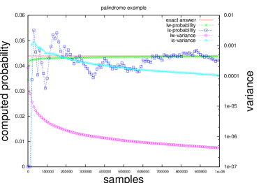
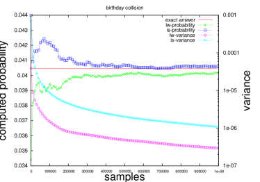
(a) Palindrome	(b) Birthday

Figure 8: Experimental Results

• Palindrome, which is shown in Fig. 1, with evidence limited to strings of length $N=20$, and query checking $K=4$ “a”s. While the compuation of evidence probability is easy, the computation of the probability for conjunction of query and evidence is not. This is because, the query searches for all possible combinations of ’K’ positions. Therefore, for large problem sizes, likelihood weighting has to be used to get approximate answers.

• Birthday, shown in Fig. 2 with population size of $6$, i.e. query same_birthday(6). While this query can be evaluated by exact inference due to measurability, we use it to test the performance of likelihood weighted sampler.

The results of the experiments are shown in Fig. 8. Each subfigure plots the estimated probability and variance of the estimate (on log scale), for two samplers: the LW method described in this paper, and a simple independent sampler (with rejection sampling for conditional queries). Note that the LW sampler’s results show significantly lower variance in both the examples.

For the Palindrome example, the LW sampler quickly converges to the actual probability, while the independent sampler fails to converge even after a million samples. The unusual pattern of variance for independent sampler in the initial iterations is due to it not being able to generate consistent samples and hence not having an estimate for the answer probability. In the birthday example, we notice that all consistent samples have the same likelihood weight and they are quite low. Due to this reason, likelihood weighting doesn’t perform much better than independent sampling. Interestingly, independent sampling using the OSDD structure was significantly faster (up to $2\times$) than using the program directly. This is because the program’s non-deterministic evaluation has been replaced by a deterministic traversal through the OSDD.

Comparison with PITA and ProbLog samplers

We compared the performance of LW sampler with the sampling based inference of ProbLog and PITA . ProbLog provides independent sampling along with an option to propagate evidence. We didn’t find these to be effective and ProbLog failed to generate consistent samples in reasonable time (5 mins). PITA sampling [Riguzzi, 2011] on the other hand provided better performance (see table 1). Due to the lack of constraint processing, the time required per sample is higher for PITA although the convergence behavior is similar. It should be noted that PITA counts only consistent samples, and there can be many attempts at generation of a consistent sample. In contrast, our constraint processing techniques allow us to generate a consistent sample at every attempt (for the specific examples considered). The plots showing estimated answer probability and the variance of the estimates for the two examples for PITA are shown in Fig. 9.

Problem	OSDD gen.	LW	ProbLog	ProbLog-pe	Mcint.-rej.	Mcint.-MH
palindrome	0.019	0.00017	188	na	0.41	7.7
birthday	0.025	1.7e-5	19	26	0.004	0.003

Table 1: Time for OSDD computation and per consistent sample (seconds)

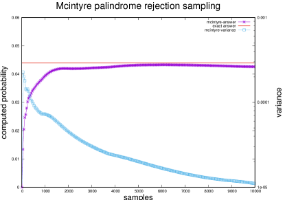
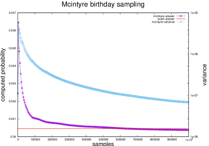
PITA palindrome	PITA birthday

Figure 9: Experimental Results for PITA samplers

PITA and ProbLog exact inference

We evaluated the exact inference procedures of PITA and ProbLog on the same examples. We used a timeout of 15 minutes for both systems. ProbLog’s inference does not scale beyond small problem sizes for thes two examples. PITA could successfully compute the conditional probabilities for Palindrome with $n=18$. PITA’s inference completed for the Birthday example with population size $2$, but ran out of memory for larger population sizes. The table 2 shows the time required to construct the OSDDs for the birthday example and the palindrome example. The leftmost column gives the population size/length of the string. While the birthday problem has a single osdd, the palindrome example requires two osdds: the one for evidence and one for conjunction of query and evidence. It turns out that all of them satisfy the measurability property. However we note that the osdd for conjunction of query and evidence for palindrome example is intractable for large problem sizes. The evidence osdd for palindrome on the other hand is very simple and scales well. The columns with title “M. prob” show the time required to compute the probability from the OSDDs by exploiting measurability.

	Birthday			Palindrome
Size	osdd	M. prob.	evid. osdd	qe osdd	M. prob
6	0.025	0.005	0.01	0.043	0.003
8	0.079	0.008	0.01	0.208	0.006
10	0.215	0.014	0.0109	0.7189	0.008
12	0.795	0.024	0.0129	1.877	0.008
14	5.49	0.035	0.014	4.94	0.033
16	52.83	0.056	0.017	16.03	0.076

Table 2: Time for OSDD generation and probability computation (seconds)

6 Related Work

Symbolic inference based on OSDDs was first proposed in [Nampally and Ramakrishnan, 2015]. The present work expands on it two significant ways: Firstly, the construction of OSDDs is driven by tabled evaluation of transformed programs instead of by abstract resolution. Secondly, we give an exact inference procedure for probability computation using OSDDs which generalizes the exact inference procedure with ground explanation graphs.

Probabilistic Constraint Logic Programming [Michels et al., 2013] extends PLP with constraint logic programming (CLP). It allows the specification of models with imprecise probabilities. Whereas a world in PLP denotes a specific assignment of values to random variables, a world in PCLP can define constraints on random variables, rather than specific values. Lower and upper bounds are given on the probability of a query by summing the probabilities of worlds where query follows and worlds where query is possibly true respectively. While the way in which “proof constraints” of a PCLP query are obtained is similar to the way in which symbolic derivations are obtained (i.e., through constraint based evaluation), the inference techniques employed are completely different with PCLP employing satisfiability modulo theory (SMT) solvers.

cProbLog extends ProbLog with first-order constraints [Fierens et al., 2012]. This gives the ability to express complex evidence in a succinct form. The semantics and inference are based on ProbLog. In contrast, our work makes the underlying constraints in a query explicit and uses the OSDDs to drive inference.

CLP($\mathcal{BN}$) [Costa et al., 2002] extends logic programming with constraints which encode conditional probability tables. A CLP($\mathcal{BN}$) program defines a joint distribution on the ground skolem terms. Queries are answered by performing inference over a corresponding BN.

There has been a significant interest in the area of lifted inference as exemplified by the work of [Poole, 2003; Braz et al., 2005; Milch et al., 2008]. The main idea of lifted inference is to treat indistinguishable instances of random variables as one unit and perform inference at the population level. Lifted inference in the context of PLP has been performed by converting the problem to parfactor representation [Bellodi et al., 2014] or weighted first-order model counting [Van den Broeck et al., 2011]. Lifted explanation graphs [Nampally and Ramakrishnan, 2016] are a generalization of ground explanation graphs, which treat instances of random processes in a symbolic fashion. In contrast, exact inference using OSDDs treats values of random variables symbolically, thereby computing probabilities without grounding the random variables. Consequently, the method in this paper can be used when instance-based lifting is inapplicable. Its relationship to more recent liftable classes [Kazemi et al., 2016] remains to be explored.

The use of sampling methods for inference in PLPs has been widespread. The evidence has generally been handled by heuristics to reduce the number of rejected samples [Cussens, 2000; Moldovan et al., 2013]. More recently, [Nitti et al., 2016] present an algorithm that generalizes the applicability of LW samples by recognizing when valuation of a random variable will lead to query failure. Our technique propagates constraints imposed by evidence. With a rich constraint language and a propagation algorithm of sufficient power, the sampler can generate consistent samples without any rejections.

Adaptive sequential rejection sampling [Mansinghka et al., 2009] is an algorithm that adapts its proposal distributions to avoid generating samples which are likely to be rejected. However, it requires a decomposition of the target distribution, which may not be available in PLPs. Further, in our work the distribution from which samples are generated is not adapted. It is an interesting direction of research to combine adaptivity with the proposed sampling algorithm.

7 Conclusion

In this work we introduced OSDDs as an alternative data structure for PLP. OSDDs enable efficient inference over programs whose random variables range over large finite domains. We also showed the effectiveness of using OSDDs for likelihood weighted sampling.

OSDDs may provide asymptotic improvements for inference over many classes of first-order probabilistic graphical models. An example of such models is the Logical hidden Markov model (LOHMM) which lifts the representational structure of hidden Markov models (HMMs) to a first-order domain [Kersting et al., 2006]. LOHMMs have proved to be useful for applications in computational biology and sequential behavior modeling. LOHMMs encode first-order relations using abstract transitions of the form $p:\mathtt{H}\xleftarrow[]{\mathtt{O}}\mathtt{B}$ where $p\in[0,1]$. Any of $\mathtt{H},\mathtt{B},\mathtt{O}$ may be partially ground, and there may be logical variables which are shared between any of the atoms in an abstract transition. Abstract explanations that are obtained by inference over such models that avoids grounding of variables whenever possible can be naturally captured by OSDDs.

Appendix A Proofs

Proposition (Closure properties).

OSDDs are closed under conjunction and disjunction operations.

Proof.

Let $\psi=(s,k,Y)[\gamma_{i}:\psi_{i}]$ and $\psi^{\prime}=(s^{\prime},k^{\prime},Y^{\prime})[\gamma^{\prime}_{j}:\psi^{\prime}_{j}]$ be two OSDDs.

Let $\oplus$ denote either $\land$ or $\lor$, then by the definition of $\psi\oplus\psi^{\prime}$ ordering is preserved. Depending on the ordering of the OSDDs, $\psi\oplus\psi^{\prime}$ has three cases. If $(s,k)\prec(s^{\prime},k^{\prime})$ (resp. $(s^{\prime},k^{\prime})\prec(s,k)$ then $\psi\oplus\psi^{\prime}$ is constructed by leaving the root and edge lables intact at $(s,k,Y)$ (resp. $(s^{\prime},k^{\prime},Y^{\prime}))$. In this case urgency, mutual exclusion, and completeness are all preserved since $\psi$ (resp. $\psi^{\prime}$) is an OSDD and the root and its edge labels are unchanged.

If $(s,k)=(s^{\prime},k^{\prime})$ urgency is preserved since $\forall i\forall j$ $\gamma_{i}\land\gamma^{\prime}_{j}$ are the constructed edges of $\psi\oplus\psi^{\prime}$ and individually these $\gamma_{i}$ and $\gamma^{\prime}_{j}$ satisfied urgency. If we take two distinct edge constraints $\gamma_{i}\land\gamma^{\prime}_{j}$ and $\gamma_{k}\land\gamma_{l}$ it is the case that $\mbox{$\mbox{$[\![$}\gamma_{i}\land\gamma^{\prime}_{j}\land\gamma_{k}\land\gamma^{\prime}_{l}\mbox{$]\!]$}$}=\emptyset$ since either $i\neq k$ or $j\neq l$ and both $\mbox{$\mbox{$[\![$}\gamma_{i}\land\gamma_{k}\mbox{$]\!]$}$}=\emptyset$ and $\mbox{$\mbox{$[\![$}\gamma^{\prime}_{j}\land\gamma^{\prime}_{l}\mbox{$]\!]$}$}=\emptyset$. Let $\sigma$ be the grounding substitution of $\cup_{i,j}Vars(\gamma_{i}\land\gamma^{\prime}_{j})\setminus\{Y\}$ that is compatible with constraint formula labeling the path to the node $(s,k,Y)$. To prove completeness, we note that $\cup_{j}\mbox{$\mbox{$[\![$}\gamma_{i}\sigma\land\gamma^{\prime}_{j}\sigma\mbox{$]\!]$}$}_{Y}=\mbox{$\mbox{$[\![$}\gamma_{i}\sigma\mbox{$]\!]$}$}_{Y}$. Therefore, $\cup_{i,j}\mbox{$\mbox{$[\![$}(\gamma_{i}\land\gamma^{\prime}_{j})\sigma\mbox{$]\!]$}$}=type(Y)$. ∎

Proposition.

Let $\psi=(s,k,Y)[\gamma_{i}:\psi_{i}]$ and $\psi^{\prime}=(s^{\prime},k^{\prime},Y^{\prime})[\gamma^{\prime}_{j}:\psi^{\prime}_{j}]$ be two OSDDs, then

$$\mathcal{G}(\psi\oplus\psi^{\prime})=\mathcal{G}(\psi)\oplus\mathcal{G}(\psi^{\prime}).$$

Proof.

When $(s,k)\prec(s^{\prime},k^{\prime})$, then $\mathcal{G}(\psi)\oplus\mathcal{G}(\psi^{\prime})=(s,k,Y)[\alpha_{r}:\mathcal{G}(\psi_{r}[\alpha_{r}/Y])\oplus\mathcal{G}(\psi^{\prime})]$. But $\mathcal{G}(\psi\oplus\psi^{\prime})=\mathcal{G}((s,k,Y)[\gamma_{i}:\psi_{i}\oplus\psi^{\prime}])=(s,k,Y)[\alpha_{r}:\mathcal{G}(\psi_{r}\oplus\psi^{\prime}[\alpha_{r}/Y])]$.

Thus, we consider the case where $(s,k)=(s^{\prime},k^{\prime})$. Both ground explanation graphs have the same root, therefore the ground explanations in $\mathcal{G}(\psi)\oplus\mathcal{G}(\psi^{\prime})$ are obtained by combining subtrees connected which have the same edge label. Given grounding substitution $\sigma$ on $\cup_{i,j}Vars(\gamma_{i}\land\gamma^{\prime}_{j})\setminus\{Y\}$ that is compatible with the constraint formula labeling the path from root to the node under consideration, if some value $\alpha\in type(Y)$ is such that it satisfies $\gamma_{i}\sigma$ and $\gamma^{\prime}_{j}\sigma$ for specific $i,j$, then in $\psi\oplus\psi^{\prime}$, $\alpha\in\mbox{$\mbox{$[\![$}(\gamma_{i}\land\gamma_{j})\sigma\mbox{$]\!]$}$}_{Y}$, therefore the same subtrees are combined. ∎

Proposition (Condition for Measurability).

A satisfiable constraint formula is measurable w.r.t all of its variables if and only if it saturated.

Proof.

First we prove that saturation is a sufficient condition for measurability.

The proof is by induction on the number of variables in $\gamma$. When $|Vars(\gamma)|=1$ the proposition holds since the only satisfiable constraint formulas with a single variable are $\{X=c\}$ for some $c\in Dom(X)$ or formulas of the form $\{X\neq c_{1},X\neq c_{2},\ldots,X\neq c_{m}\}$ for some distinct set of values $\{c_{1},\ldots,c_{m}\}\subset Dom(X)$. Clearly the formulas are measurable w.r.t $X$.

Assume that the proposition holds for saturated constraint formulas with $n$ variables. Now consider a satisfiable constraint formula $\gamma$ with $n+1$ variables which is saturated. Let $X\in Vars(\gamma)$. Consider the graph obtained by removing $X$ and all edges incident on $X$ from the constraint graph of $\gamma$. It represents a saturated constraint formula $\gamma^{\prime}$ with $n$ variables. This is because for any three variables $A,B,C$ distinct from $X$, if $A=B,B=C$ then $A,C$ are connected by an “$=$” edge. Similarly, if $A=B,B\neq C$, then $A,C$ are connected by an “$\neq$” edge. Further for any variable $A$ other than $X$, if $Z$ is the set of variables connected to $A$ by “$\neq$” edges, then there exists edges between each pair of these nodes. This is due to the definition of saturation which is satisfied by $\gamma$.

But, by inductive hypothesis $\gamma^{\prime}$ is measurable w.r.t each of its variables. Now consider computing the measure of $X$ in $\gamma$. If $X$ is connected to any node $Y$ with an “$=$” edge, then measure of $X$ is 1. If $X$ is not connected to any node with an “$=$” edge, then it is either disconnected from other nodes or connected to them by only “$\neq$” edges. In either case $m_{X}$ is computed by subtracting the number of nodes connected to $X$ by “$\neq$” edges from the domain.

To prove that saturation is a necessary condition we use proof by contradiction. Assume there exists a measurable constraint formula $\gamma$ which is not saturated. Then there exists a variable $X\in Vars(\gamma)$ and a set $\mathcal{Z}$ which is the set of nodes connected to the node for $X$ by “$\neq$” edge and for some pair of elements $A,B\in\mathcal{Z}$, there is no edge between them. Since we take closure of “$=$” edges, we can assume that $\gamma\not\models A=B$. So there must exist two substitutions $\sigma,\sigma^{\prime}$ where $A=B$ and $A\neq B$ respectively. The number of solutions of $X$ under these two substitutions is clearly different, which is a contradiction. ∎

References

- Bellodi et al. [2014] Bellodi, E., Lamma, E., Riguzzi, F., Costa, V. S., and Zese, R. 2014. Lifted variable elimination for probabilistic logic programming. TPLP 14, 4-5, 681–695.
- Braz et al. [2005] Braz, R. D. S., Amir, E., and Roth, D. 2005. Lifted first-order probabilistic inference. In 19th Intl. Joint Conf. on Artificial intelligence. 1319–1325.
- Bryant [1992] Bryant, R. E. 1992. Symbolic boolean manipulation with ordered binary-decision diagrams. ACM Computing Surveys 24, 3, 293–318.
- Costa et al. [2002] Costa, V. S., Page, D., Qazi, M., and Cussens, J. 2002. CLP(BN): Constraint logic programming for probabilistic knowledge. In 19th Conf. on Uncertainty in Artificial Intelligence. 517–524.
- Cussens [2000] Cussens, J. 2000. Stochastic logic programs: Sampling, inference and applications. In 16th Conf. on Uncertainty in Artificial Intelligence. Morgan Kaufmann, 115–122.
- De Raedt et al. [2007] De Raedt, L., Kimmig, A., and Toivonen, H. 2007. Problog: A probabilistic Prolog and its application in link discovery. In 20th Intl. Joint Conf. on Artifical Intelligence. 2462–2467.
- Fierens et al. [2012] Fierens, D., Van den Broeck, G., Bruynooghe, M., and De Raedt, L. 2012. Constraints for probabilistic logic programming. In NIPS Probabilistic Programming Workshop. 1–4.
- Fung and Chang [1990] Fung, R. M. and Chang, K.-C. 1990. Weighing and integrating evidence for stochastic simulation in bayesian networks. In 5th Annual Conf. on Uncertainty in Artificial Intelligence. 209–220.
- Geman and Geman [1984] Geman, S. and Geman, D. 1984. Stochastic relaxation, Gibbs distributions, and the Bayesian restoration of images. IEEE Transactions on Pattern Analysis and Machine Intelligence 6, 6, 721–741.
- Hastings [1970] Hastings, W. 1970. Monte carlo sampling methods using markov chains and their applications. Biometrika 57, 1, 97–109.
- Holzbaur [1992] Holzbaur, C. 1992. Metastructures versus attributed variables in the context of extensible unification. In 4th Intl. Symp. on Programming Language Implementation and Logic Programming. 260–268.
- Kam et al. [1998] Kam, T., Villa, T., Brayton, R., and Sangiovanni-Vincentelli, A. 1998. Multivalued decision diagrams: Theory and applications. Intl. J. Multiple-Valued Logic 4, 9–62.
- Kazemi et al. [2016] Kazemi, S. M., Kimmig, A., Broeck, G. V. d., and Poole, D. 2016. New liftable classes for first-order probabilistic inference. In NIPS. 3125–3133.
- Kersting et al. [2006] Kersting, K., Raedt, L. D., and Raiko, T. 2006. Logical hidden Markov models. Journal of Artificial Intelligence Research 25, 2006.
- Mansinghka et al. [2009] Mansinghka, V. K., Roy, D. M., Jonas, E., and Tenenbaum, J. B. 2009. Exact and approximate sampling by systematic stochastic search. In 12th Intl. Conf. on A. I. and Statistics. 400–407.
- Michels et al. [2013] Michels, S., Hommersom, A., Lucas, P. J., Velikova, M., and Koopman, P. 2013. Inference for a new probabilistic constraint logic. In 23rd Intl. Joint Conf. on Artificial Intelligence. 2540–2546.
- Milch et al. [2008] Milch, B., Zettlemoyer, L. S., Kersting, K., Haimes, M., and Kaelbling, L. P. 2008. Lifted probabilistic inference with counting formulas. In 23rd AAAI Conf. on Artificial Intelligence. 1062–1068.
- Moldovan et al. [2013] Moldovan, B., Thon, I., Davis, J., and Raedt, L. D. 2013. MCMC estimation of conditional probabilities in probabilistic programming languages. In ECSQARU. 436–448.
- Nampally and Ramakrishnan [2015] Nampally, A. and Ramakrishnan, C. R. 2015. Constraint-based inference in probabilistic logic programs. In 2nd Intl. Workshop on Probabilistic Logic Programming. 46–56.
- Nampally and Ramakrishnan [2016] Nampally, A. and Ramakrishnan, C. R. 2016. Inference in probabilistic logic programs using lifted explanations. In 32nd Intl. Conf. on Logic Programming, ICLP 2016 TCs. 15:1–15:15.
- Nitti et al. [2016] Nitti, D., De Laet, T., and De Raedt, L. 2016. Probabilistic logic programming for hybrid relational domains. Machine Learning 103, 3, 407–449.
- Poole [2003] Poole, D. 2003. First-order probabilistic inference. In 18th Intl. Joint Conf. on A. I. 985–991.
- Riguzzi [2011] Riguzzi, F. 2011. MCINTYRE: A Monte Carlo algorithm for probabilistic logic programming. In CILC. 25–39.
- Riguzzi and Swift [2011] Riguzzi, F. and Swift, T. 2011. The PITA system: Tabling and answer subsumption for reasoning under uncertainty. Theory and Practice of Logic Programming (TPLP) 11, 4-5, 433–449.
- Sarna-Starosta and Ramakrishnan [2007] Sarna-Starosta, B. and Ramakrishnan, C. R. 2007. Compiling constraint handling rules for efficient tabled evaluation. In Practical Aspects of Declarative Languages (PADL). 170–184.
- Sato and Kameya [1997] Sato, T. and Kameya, Y. 1997. PRISM: A language for symbolic-statistical modeling. In 15th Intl. Joint Conf. on Artificial Intelligence. 1330–1339.
- Sato and Kameya [2001] Sato, T. and Kameya, Y. 2001. Parameter learning of logic programs for symbolic-statistical modeling. Journal of Artificial Intelligence Research 15, 391–454.
- Shachter and Peot [1990] Shachter, R. D. and Peot, M. A. 1990. Simulation approaches to general probabilistic inference on belief networks. In 5th Annual Conf. on Uncertainty in Artificial Intelligence. 221–234.
- Swift and Warren [2010] Swift, T. and Warren, D. S. 2010. Tabling with answer subsumption: Implementation, applications and performance. In Logics in Artificial Intelligence: 12th European Conference (JELIA). 300–312.
- Tamaki and Sato [1986] Tamaki, H. and Sato, T. 1986. OLD resolution with tabulation. In Proceedings of the Third international conference on logic programming. Springer, 84–98.
- Van den Broeck et al. [2011] Van den Broeck, G., Taghipour, N., Meert, W., Davis, J., and De Raedt, L. 2011. Lifted probabilistic inference by first-order knowledge compilation. In Proceedings of the Twenty-Second international joint conference on Artificial Intelligence. 2178–2185.