Halo Profiles and the Concentration–Mass Relation for a CDM Universe
Abstract
Profiles of dark matter-dominated halos at the group and cluster scales play an important role in modern cosmology. Using results from two very large cosmological -body simulations, which increase the available volume at their mass resolution by roughly two orders of magnitude, we robustly determine the halo concentration–mass – relation over a wide range of masses, employing multiple methods of concentration measurement. We characterize individual halo profiles, as well as stacked profiles, relevant for galaxy–galaxy lensing and next-generation cluster surveys; the redshift range covered is , with a minimum halo mass of . Despite the complexity of a proper description of a halo (environmental effects, merger history, nonsphericity, relaxation state), when the mass is scaled by the nonlinear mass scale , we find that a simple non-power-law form for the – relation provides an excellent description of our simulation results across eight decades in and for . Over the mass range covered, the – relation has two asymptotic forms: an approximate power law below a mass threshold , transitioning to a constant value, at higher masses. The relaxed halo fraction decreases with mass, transitioning to a constant value of above the same mass threshold. We compare Navarro–Frenk–White (NFW) and Einasto fits to stacked profiles in narrow mass bins at different redshifts; as expected, the Einasto profile provides a better description of the simulation results. At cluster scales at low redshift, however, both NFW and Einasto profiles are in very good agreement with the simulation results, consistent with recent weak lensing observations.
1 Introduction
The endpoints of structure formation in cold dark matter cosmologies are dark matter-dominated clumps called halos. In these cosmologies, initial density perturbations are amplified by the gravitational Jeans instability and small localized nonlinear structures form at high redshift. As the universe evolves, halos grow via mass accretion and halo mergers; galaxies form within halos. Halo abundance, evolution history, and properties such as mass, velocity, sub-structure, and phase space structure, as well as the halo gas and galaxy content, all play important roles in modern cosmology, as well as in the modeling of galaxy formation, whether by empirical or semi-analytic means (White & Frenk, 1991; Kauffmann et al., 1993, 1997; Cole et al., 1994; Jing et al., 1998; Somerville & Primack, 1999; Benson et al., 2000, 2003; Peacock & Smith, 2000; Seljak, 2000; Berlind & Weinberg, 2002; Vale & Ostriker, 2004; Zheng et al., 2005; Baugh, 2006; Conroy et al., 2006; Benson, 2010; Guo et al., 2010; Moster et al., 2010; Wetzel & White, 2010; Hearin et al., 2016). A number of observational probes based on strong and weak gravitational lensing, X-ray observations, and galaxy clustering are sensitive to the nature of halo density profiles (Meneghetti et al., 2005; Mandelbaum et al., 2006, 2008; Comerford & Natarajan, 2007; Johnston et al., 2007; Okabe et al., 2010, 2013; Umetsu et al., 2011, 2014, 2016; Oguri et al., 2012; Bhattacharya et al., 2013; Newman et al., 2013; Merten et al., 2015; Niikura et al., 2015; Amodeo et al., 2016; Okabe & Smith, 2016; Umetsu & Diemer, 2017). This is particularly true for cluster cosmology and galaxy–galaxy lensing, which focus at the upper end of the halo mass range.
In the remainder of the introduction, we briefly discuss halo profiles and concentrations and their importance for cosmology (Section 1.1), the current state of observed halo profiles (Section 1.2), and prior work on the profiles and concentrations of simulated halos (Section 1.3). We then outline the aims and primary results of this work (Section 1.4).
1.1 Halo Profiles
Although the formation of halos is a complex, hierarchical nonlinear dynamical process, the radial density profile of individual halos is robustly fit by a surprisingly simple form, as first described by Navarro, Frenk, & White (1996, 1997), using results from cosmological -body simulations. The two-parameter NFW density profile is given by
| (1) |
where is a characteristic dimensionless density parameter. The critical density is ; is the Hubble parameter, and the NFW scale radius, , is defined by the radius where the logarithmic profile slope . For , , whereas for , . A dimensionless shape parameter, the halo concentration, , is commonly used as one of the NFW parameters. The halo radius is a radial scale set by the spherical overdensity (SO) halo mass definition: , where is a dimensionless overdensity parameter. We choose the critical density as the reference density; the mean density of the universe is another common choice. We also make the conventional choice of (for X-ray work with clusters, higher values of are often used, such as or ), and refer to the corresponding concentration as .
Describing individual halos in terms of the NFW description is obviously a severe idealization. Halos are not spherical and can have complex shapes. In particular, a more realistic description of individual halos is as prolate ellipsoids with a major axis length roughly twice as long as the minor axis (Jing & Suto, 2002). Additionally, at a fixed halo mass and more or less independent of the how the mass is defined, halo shapes and profiles can display considerable variability, with some dependence on whether the halos are dynamically relaxed (White, 2002; Lukić et al., 2009). Observations that focus on stacked halos, such as galaxy–galaxy lensing or stacked cluster weak lensing, involve averaging over many individual halos and thus reduce bias due to the characteristics of individual lenses (see, e.g., Simet et al. 2017 as an example of the current state of the art).
Despite some of these caveats, there are well-defined and observationally testable predictions for halo masses and profiles as a function of cosmological parameters. For instance, the halo mass function is an essential cosmological quantity, relevant to determining cluster abundance (Holder et al., 2001) and to modeling of the observed galaxy distribution, to mention two obvious examples. The halo profile shape can also be predicted accurately in modern cosmological simulations and is known to be correlated with the halo mass. One aspect of this correlation is the existence of a well-determined – relation, as was already noted by NFW. Cosmological constraints delivered by ongoing surveys such as the Dark Energy Survey (DES111https://www.darkenergysurvey.org) and next-generation surveys such as the Dark Energy Spectroscopic Instrument (DESI222http://desi.lbl.gov), Euclid (Refregier et al. 2010), the Large Synoptic Survey Telescope (LSST) (LSST Science Collaboration et al. 2009), and the Wide-field Infrared Survey Telescope (WFIRST) (Spergel et al. 2015) will rely on having accurate predictions for halo profiles and masses.
1.2 Observed Profiles: Individual and Stacked Halos
Individual halo profiles can be measured using X-ray and strong and weak lensing measurements, as already mentioned. Because of a number of factors (e.g., observational limitations, selection bias, individual variability, line-of-sight dependence, analysis issues), there are difficulties in comparing these observations directly to theoretical predictions. Earlier measurements tended to have higher concentrations and a significantly steeper – relation than that predicted by simulations (see, e.g., Schmidt & Allen 2007; Broadhurst et al. 2008; Okabe et al. 2010; Oguri et al. 2012 and the discussion in Comerford & Natarajan 2007); however, the state of the art has been significantly enhanced by more recent group and cluster-scale observations. In Figure 1 we present a set of recent observational results for the – relation from measurements of individual clusters. (For another compilation, see Bhattacharya et al. 2013.) We also show results from the simulation carried out in this paper, which are discussed in detail in Section 4.1 below; we find good agreement between the observations and the CDM predictions, despite uncertainties in accounting for selection biases and other measurement errors.

Given sufficient statistics, stacking techniques can be used for both higher- (cluster weak lensing) and lower-mass halos (galaxy–galaxy lensing). The results from stacked observations average over intrinsic halo variability and lines of sight, but have different systematic issues compared to individual halo measurements. Moreover, stacked density profiles differ systematically from the NFW prescription, with potentially observable consequences. As discussed in Section 3.2, the Einasto profile (Einasto, 1965) is a much better fit in this case. Next-generation surveys, and LSST in particular, will increase the number of known clusters by over an order of magnitude. Provided systematic errors can be sufficiently controlled, there is, therefore, sufficient motivation to consider the individual and stacked halo profiles separately. Figure 2 shows observational results for stacked observations using galaxy–galaxy lensing and cluster weak lensing. Here too, the results are in good agreement; significant improvements in the observational results are expected in the near future.

1.3 Concentrations of Simulated Halos
Even without including baryonic effects, which at cluster-scale masses could lead to changes at the level (Duffy et al., 2010), the current status of theoretical predictions and comparison with observations as shown in Section 4.1 is certainly satisfactory. However, a number of open issues still remain. Simulations have shown that the concentration depends on both mass and redshift, with massive halos less concentrated than lower-mass halos at the same redshift. The – relation has been measured in a large number of papers, in different ways (Bullock et al. 2001; Eke et al. 2001; Zhao et al. 2003; Duffy et al. 2008; Gao et al. 2008; Macciò et al. 2008; Klypin et al. 2011, 2016; Ludlow et al. 2012, 2014, 2016; Prada et al. 2012; Bhattacharya et al. 2013; Correa et al. 2015; and Diemer & Kravtsov 2015). There has been some disagreement in the results obtained, which appears to be largely due to the different ways in which the concentration has been operationally defined. Different fitting methods and binning choices can produce inconsistent – relations (see, e.g., discussions in Bhattacharya et al. 2013; Meneghetti & Rasia 2013; Dutton & Maccio 2014). One of the objectives of this paper, therefore, is to present a robust set of results, arrived at by using methods with potentially different systematics, and by investigating several possible sources of numerical error.
1.4 This Work
The primary aim of this paper is to further study and robustly determine the – relation and halo profiles at group and cluster scales at low to medium redshifts, and to characterize the profile evolution over this redshift range for both relaxed and unrelaxed halos. The halo mass range considered here is mostly focused on masses significantly larger than the nonlinear (or “collapse”) mass scale , which gives the mass scale corresponding to peaks of the initial Gaussian random field collapsing at redshift (see definition in Section 4): at , at , and at . Following the discussion above, we split our – relation study into two parts: one for individual halos and the other for stacked halos, in order to be consistent with current and future observational strategies.
We determine the concentration by fitting the radial mass distribution, , rather than the density profile, following the procedure outlined in Bhattacharya et al. (2013). In addition to this primary method, we introduce two alternative techniques for concentration estimation – one of which is independent of the assumed form of the density profile – that we employ to characterize the robustness with which the – relation can be determined. We find that the results are in good agreement over the mass ranges where all of our methods can be properly used. Each of the three methods is sensitive to a different range of the profile, and subject to different types of error – we use the agreement across methods to show that our concentration measurements are robust.
The two massive state-of-the-art CDM simulations (Section 2) that form the basis of the results presented here share two essential characteristics: large volumes and very good mass resolution. At the mass resolutions considered, these simulations have roughly two orders of magnitude more volume than previous work. This allows us to robustly explore the – relation with excellent statistics over a relatively wide halo mass and redshift range, and to use narrow mass bins in stacked analyses. Our results are consistent with the general idea that the concentration of halos should be set more or less by the mean density of the universe when the halos are assembled. (Unfortunately, there is no predictive theory for how the – relation should depend on redshift, because there is no real theory for the NFW profile either.) At , massive clusters, which are still forming today, would be expected to have a lower concentration than smaller-mass halos that have masses less than . Because drops steeply with redshift, at , one might expect the – relation to flatten over a significantly extended mass range as redshift increases and a large fraction of the halos in the upper mass range are still forming. Our results are very consistent with this expectation.
By combining results from multiple redshifts and scaling the halo mass by the nonlinear mass scale , we find that the – relation can be well-fit by a single expression; in agreement with Zhao et al. (2003), Gao et al. (2008), Ludlow et al. (2014), we find a concentration floor of . The transition from a power-law behavior of the scaled – relation to an asymptotically flat regime occurs at a halo threshold mass, , right at the upper end of cluster-scale halo masses at . We note that the unrelaxed halo fraction is roughly half at masses above , and decreases with mass below . Further discussion of these results can be found in Section 4.
As is a function of cosmological parameters, we can compare our results to other simulations in the same family of CDM cosmologies by assuming a certain level of universal behavior, as is known to hold for the mass function (see, e.g., Heitmann et al. 2006). Appendix A.2 shows that the – relations of other simulations fall within the population variance of our results, and their results from redshifts between and broadly follow the shape of a power-law transitioning to constant . We have checked that this cosmology-independent behavior does not hold sufficiently far away from our fiducial cosmology by comparison to the CDM results presented in Bhattacharya et al. (2013) and in Kwan et al. (2013).
The rest of this paper is organized as follows. In Section 2, we describe the large cosmological -body simulations that are the source of the halo catalogs and halo profiles. Section 3 describes our methodology for measuring the halo concentrations using the radial profiles. Section 4 presents the resulting – relations and the new fitting form using scaled halo masses. Section 5 concludes with a final discussion of the results. The appendices contains the results of investigations of possible sources of numerical error and comparisons of some of our results to previous work.
2 Simulations
The results reported here use data from two very large, gravity-only -body simulations run with the Hardware/Hybrid Accelerated Cosmology Code (HACC) framework (Habib et al., 2016). These are the ‘Q Continuum’ (Heitmann et al., 2014) and ‘Outer Rim’ (Habib et al., 2016) simulations carried out on the CPU/GPU system Titan at Oak Ridge National Laboratory and the Blue Gene/Q (BG/Q) system Mira at Argonne National Laboratory, respectively. HACC uses a hybrid force calculation scheme, splitting the total force calculation into a long-range component and a short-range component. In both runs, the long-range forces are computed using the same high-order spectral particle mesh method, while the short-range forces are computed using different methods (albeit with the same hand-over scale to the short-range solver) in order to best exploit the available computational architecture. A direct particle-particle interaction technique is used for the CPU/GPU system and an RCB (Recursive Coordinate Bisection) tree method for the BG/Q system. Halo identification and characterization is carried out with HACC’s parallel CosmoTools analysis framework, using a combination of in situ and offline analyses.
The Q Continuum and Outer Rim runs represent independent realizations of the same shared WMAP-7 (Komatsu et al., 2011) cosmology:
| (2) |
but with differing volumes and mass resolution. The box size for the Q Continuum run is , while that of Outer Rim is . The number of particles in these simulations are trillion (Q Continuum) and trillion (Outer Rim); the associated mass resolutions are (Q Continuum) and (Outer Rim). The force resolutions are (comoving) (Q Continuum) and (Outer Rim). Both simulations are given a Zel’dovich approximation initial condition at with transfer functions generated by the CAMB code (Lewis et al., 2000). The Outer Rim simulation has been used for several analyses of SDSS IV extended Baryon Oscillation Spectroscopic Survey data (Gil-Marín et al., 2018; Hou et al., 2018; Zarrouk et al., 2018).
The large volumes and excellent mass resolution in these simulations lead to the following advantages in characterizing halo properties: (1) sufficiently large numbers of halos at high masses over the redshift ranges studied (at , million and million halos of at least 2000 particles in Q Continuum and Outer Rim, respectively); (2) excellent profile resolution for individual halos; and (3) the ability to study stacked halo profiles in narrow mass bins – hundreds of halos in mass bins of width at cluster scales, and hundreds of thousands at lower masses. Compared to our previous work in Bhattacharya et al. (2013), the mass resolution is improved by more than an order of magnitude. In addition, the overlapping volume and mass resolution coverage between the two boxes (which are run using different -body algorithms) provides an automatic cross-check for certain types of systematic errors that can arise in cosmological simulations.
3 Concentration Measurement
In this section, we describe our methods for measuring halo concentrations. This requires first defining and measuring the halo mass, followed by a determination of the halo concentration. In the context of the – relation, the mass is usually defined in terms of an SO, , as discussed in Section 1. A halo with mass has a corresponding size, , the radius within which the halo has an average overdensity of with respect to . Common choices of include and , where follows from the spherical top-hat collapse model. It is also not uncommon to define the overdensity with respect to the mean density of the universe, rather than the critical density. As stated earlier, we will use the critical density as the reference, with . It should be noted that the definition of the SO mass does not depend on the nature of the density profile.
A common alternative NFW parameterization, which we use here, describes the NFW profile in terms of an SO halo mass and the halo concentration, . Written in terms of the SO radius and the concentration, the NFW profile becomes
| (3) |
where .
Using the NFW profile as defined by Equation 3, it is clear that given (or equivalently, ) and (or equivalently, ), the NFW profile is uniquely determined. Given the NFW description, the SO mass and concentration together completely determine the spherically averaged halo profile.
Halo concentrations are computed using halo profiles built by HACC’s parallel SO halo finder, which is part of the CosmoTools analysis framework. First, friends-of-friends (FOF) halos with dimensionless linking length are found by a fast, parallel, tree-based algorithm, and their centers determined by finding the deepest potential minimum within the FOF halo. All particles (not just those in the original FOF halo) are counted in radial shells centered on the point of minimum potential, and the mass is calculated as the mass within a sphere whose average density is 200 times the critical density. No unbound particles are removed because we are interested in the density profile as measured and not in some idealized theoretical notion of what might constitute membership in a halo. Twenty shells are placed uniformly in log space between a minimum radius at the smoothing scale and a maximum radius greater than , and the differential mass profile is calculated from the bin widths and particle counts. We note that the notion of an SO halo becomes problematic during major halo mergers; the halo center is also potentially not well-defined during such epochs.
The concentration measurement procedure uses three different methods, explained in detail below: profile fit (as in Bhattacharya et al. 2013), accumulated mass, and peak finding. The idea behind using these different methods is to explore the robustness with which the concentration can be determined in the presence of different types of systematic errors. We measure concentrations only for well-sampled halos, i.e., those above a conservative threshold of at least 2000 particles within (see Appendix B.6), corresponding to a mass of for Q Continuum and for Outer Rim.
Following standard practice, for all three methods we keep the mass fixed as found by the SO algorithm described above and fit only for the concentration. In principle, it is possible to allow both quantities to float, but this leads to variability in the determined concentrations, even if the associated changes only by a small amount.
3.1 Individual Halos
Halos are dynamically evolving objects; a halo profile may not be well-described by the NFW profile if it is far from a dynamically relaxed state – for example, if it is the product of a recent merger. We identify these halos by a simple test (Neto et al., 2007; Duffy et al., 2008): halos are labeled relaxed if the distance between the halo center and the center of mass of all particles in the SO halo is, at most, . If the offset exceeds , the halo is assumed to be unrelaxed. (In rare circumstances, characterized by accidental symmetry, unrelaxed halos can pass the relaxed halo test, but the reverse is not true.) At , of all halos of at least 2000 particles are relaxed, with a higher fraction of high-mass halos unrelaxed. As redshift increases, the relaxed fraction drops to 45%, and by is independent of mass across the range (see Figure 3).
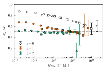
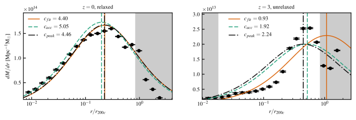
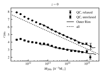
Figure 4 shows examples of relaxed and unrelaxed halo profiles at high and low redshifts. Note that much of the mass of the unrelaxed halo is far from the center, so the identified scale radius is large and concentration is small. In general, our relaxation criterion implies that unrelaxed halos have significant mass far from the potential minimum, so we expect and find unrelaxed halos to be less concentrated than relaxed halos of the same mass (Figure 5). The unrelaxed halo – relation has lower amplitude and slope than the – relation of all halos, but as for relaxed halos, concentration decreases with mass at low redshift and is constant at high . Notably, this holds true at high masses and redshifts – the relaxed halo – relation does not fall below the – relation for unrelaxed halos.
Individual halos are fit to the NFW differential mass profile,
| (4) |
which rises as at small , peaks at , and falls off as using the following three methods:
Profile Fit, . The halo mass and radius are fixed by as found by the SO algorithm. The profile fit uses the Levenberg–Marquardt algorithm, which, weighted by the Poisson error in the number of particles in each shell, minimizes
| (5) |
where is the radial width of a shell that contains particles and is evaluated at the midpoint of the bin. Only shells whose outer radius falls within and encloses at least 100 particles are fit. Shells beyond , with their high particle counts and low Poisson error, would have disproportionate influence on the fit, and the NFW form does not necessarily hold at the farther edges of a halo. The requirement of at least 100 particles in a shell also excludes the inner regions (roughly a tenth of the virial radius at cluster mass scales) that may suffer from numerical errors and not be modeled well by gravity-only simulations (due to missing baryonic/feedback effects).
Accumulated Mass, . This method uses the fact that the mass enclosed by the NFW scale radius is
| (6) |
The concentration is found iteratively by fixing , interpolating the enclosed mass profile to solve Equation (6) for , and updating .
Peak Finding, . The differential mass profile, Equation (4), peaks at , so the scale radius can be measured by simply locating the peak. To do this, profiles are smoothed using a three-point Hanning filter
| (7) |
and the scale radius is set to the location of maximum smoothed , excluding the first and last radial bins. Note that this method makes no assumption about the specific form (NFW, Einasto, etc.) of the halo profile.
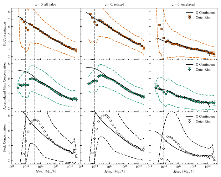
Our goal in using three different methods is to verify the robustness of our concentration measurements. These three methods are sensitive to different features of the profile. Both the profile fit and accumulated mass methods assume the NFW form, while peak finding does not. The accumulated mass method counts particles only to the scale radius, so it is most sensitive to the inner profile, . The profile fit is more influenced by the outer profile, as the outer shells, with their higher particle counts, have lower Poisson error and are weighted more heavily in the fit. If halos were always well-described by the NFW form, all three methods would find the same concentration; when their results differ, the profile is not a perfect NFW profile. We use as the primary concentration measurement and the other two methods to check our results and to better understand changes in halo profiles with mass and redshift.
The three methods agree best on well-resolved halos at low redshift, as shown in Figure 6. At high redshift, the methods differ by as much as 10%: the fit and peak concentrations are essentially flat as a function of mass, while the accumulated mass – relation slopes slightly upward, still well within the range of the intrinsic concentration scatter.

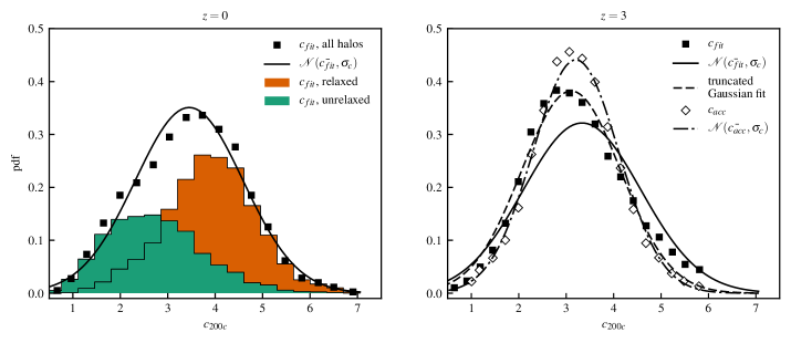
At all mass ranges and redshifts with sufficient halos in a bin, the distribution of accumulated mass concentrations is approximately normal, as shown in Figure 7. The accumulated mass scale radius can only fall between the innermost bin in the profile and , limiting the range of . However, fit concentrations can be arbitrarily high, so the distribution of is positively skewed, particularly at masses and redshifts where profiles are less well-described by the NFW form. See also Appendix A.4.
3.2 Stacked Halos
Individual halo profiles can be noisy, but with 10 million halos of at least 2000 particles at in Q Continuum and 20 million in Outer Rim, we can stack thousands of halos in a narrow mass bin (for example, , hereafter “a 1% stack”) to obtain smooth profiles. Relaxed halos are stacked by interpolating and summing the individual enclosed mass profiles. The differential mass profile is calculated from the mean enclosed mass profile. Note that we fit the 3D halo profile; a future paper will compare the concentrations that would be found for the same stacks using observational methods like weak lensing, which must fit the 2D projected mass profile.
Assuming the particles in our simulated profiles are drawn from a true NFW distribution, the stacked profile is a sum of NFW profiles with different concentrations, which, in principle, is not describable as an NFW profile. To visualize how the stacked profiles compare to an NFW profile, we calculate the effective power-law index of , that is, the slope of . For an NFW profile,
| (8) |
the density is proportional to at small and at large , crossing at the scale radius. We calculate for stacked halos using a low-noise Lanczos differentiator with ,
| (9) |
for the first two and last two bins,
| (10) | |||
| (11) |
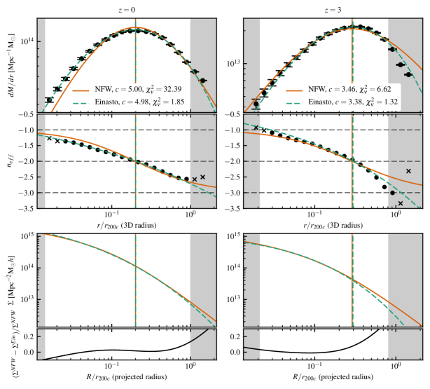
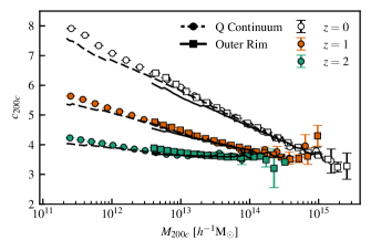
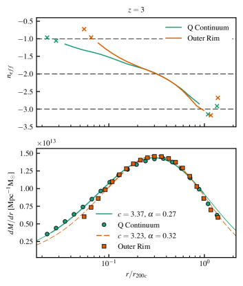
Figure 8 shows examples of stacked profiles and their at and . At high redshifts, the outer and inner profiles diverge from an NFW profile: by , density falls off more steeply than the NFW profile, while at small , the density profile becomes shallower than the NFW profile (due to limitations imposed by force and mass resolution; however, results from our two simulations are still in good agreement, indicating little effect on the concentration itself). When we nevertheless calculate the NFW concentrations of the stacks, the three methods can find different concentrations, despite their agreement on the average concentration of individual halos. Additionally, the stacked fit concentrations differ from mean individual fit concentrations, as shown in Figure 9, but by no more than 5%,. The stacked concentrations are lower than individual means at low mass, but higher at high mass. These discrepancies reflect the fact that these stacked profiles deviate from the NFW form.
Previous studies have shown that profiles with a third parameter can better fit stacked profiles (Navarro et al., 2004; Merritt et al., 2006; Prada et al., 2006; Gao et al., 2008). After investigating several three-parameter profiles, we find the Einasto profile,
| (12) |
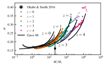
to be the best. We fit stacked halos to the Einasto form, allowing the concentration and the shape parameter to vary freely. The mass is the mean mass of halos in the stack, as determined by the SO algorithm. We find that the Einasto shape parameter increases with mass and redshift, as shown in Figure 10. These results are in reasonable agreement with the model of Gao et al. (2008) fit to results at . The Einasto concentrations agree between the Outer Rim and Q Continuum runs, but the shape parameters differ at high redshift. See Appendix B.4 for further discussion of this discrepancy, and Appendix A.5 for further comparison to other works.
Our results show that, at low mass, the stacked peak is to the left of the peak of the NFW profile fit to the stack, while at high masses at high redshift the opposite is true. At , Einasto concentrations are greater than NFW concentrations at low mass; the Einasto and NFW – relations cross around (see Figure 8 for an example stack whose peak location is well captured by the NFW fit), and at the highest masses, the Einasto concentration begins to fall below the NFW concentration. Luckily, at cluster scales at , the NFW fit peak is transitioning from the left of the stacked peak to the right, and appears to be temporarily in agreement – so NFW and Einasto profiles both fit the stacks very well, as found for the CLASH dataset by Umetsu & Diemer (2017). These authors stack profiles in a wide mass bin; we do not find substantial differences in the quality of NFW vs. Einasto fits for wide mass bins, of up to 70%, compared to narrower 1% or 5% bins.
4 The Concentration–Mass Relation
The concentration measurements described above are now used to investigate the – relation. As shown in Figures 6 and 9, the – relation flattens with increasing redshift. At higher redshifts, halos of all masses have concentration and the – relation falls no further; Zhao et al. (2003) found a similar floor. We do not present results for redshifts higher than (see discussion in the appendix), but concentrations measured up to redshifts as high as are consistent with this floor.
In order to represent the data in a -independent form, we scale the mass by the redshift-dependent nonlinear (or “collapse”) mass scale , which solves
| (13) |
where is the linear critical density for collapse and , the amplitude of mass fluctuations, is the power spectrum smoothed with a top-hat filter. The power spectrum is calculated from the growth factor
| (14) |
| (15) |
and is as given by CAMB (Lewis et al., 2000). The mean square perturbation is
| (16) |
where we choose the window function to be the Fourier transform of a spherical top-hat filter of radius ,
| (17) |
The nonlinear mass depends weakly on cosmology and falls steeply with redshift: for our cosmology, at , at , and at . Already at , , and our least-massive halos exceed the nonlinear mass scale by three orders of magnitude at this redshift. Combining the results of the two simulations at redshifts up to , we probe eight decades in , as shown in Figure 11.

When represented in terms of , the individual – relations at different redshifts fall relatively tightly onto a single relation: the concentration behaves as a power law with as long as ; at masses farther above the nonlinear mass scale, the concentration asymptotes to a constant value . This behavior is shown in Figure 11 for both individual and stacked halos, and is consistent with analytic models which find concentration to be independent of mass above a threshold mass. Dalal et al. (2010) find concentration to approach a constant for high-mass halos, those for which (implying ), where Gaussian statistics are a good description of the slopes of the corresponding peaks in the initial Gaussian random field. Okoli & Afshordi (2016), similarly, predict a constant – relation, , in the high-mass regime where an assumption of spherical collapse is valid. See further discussion in Appendix A.2.
We fit to a simple functional form that captures this behavior:
| (18) |
transitioning at from a power law to a constant . This plateau is found at a concentration between 3 and 4, depending on the halos included (all halos vs. relaxed halos only, for example) and the type of fit. Table 1 gives the fit parameters. We note that the fit should not be naïvely extrapolated to masses smaller than those considered here.
This form is not fully universal in the sense of being approximately cosmology-independent, as can be shown by checking against the CDM results of Bhattacharya et al. (2013) and Kwan et al. (2013). We are currently investigating the detailed cosmology dependence of the – relation using the Mira–Titan Universe suite of simulations (Heitmann et al., 2016; Lawrence et al., 2017), which cover 100 cosmological models allowing for a parameterization of dark energy as well as the effect of massive neutrinos. These results will be presented elsewhere.
The peak-height parameter is frequently used to find a redshift-independent – relation, with similar motivations (see, e.g. Bhattacharya et al. 2013; Dutton & Maccio 2014; Ludlow et al. 2014; Diemer & Kravtsov 2015). We find our results to be more universal with redshift as a function of than as a function of (see Appendix A.5 for further details). Moreover, we find -independence to hold for other overdensities, although it does deteriorate for smaller choices of (including ).
| Type of Fit | ||||
|---|---|---|---|---|
| Individual, all | ||||
| Individual, relaxed | ||||
| Stack, NFW | ||||
| Stack, Einasto | ||||
| Notes. Use Equation 18 with variance . | ||||
Aside from the concentration, it is also important to investigate the fraction of relaxed halos as a function of . Because halos with are likely to be in the “halo formation” phase, the unrelaxed fraction should increase with mass. However, one would anticipate that the existence of a finite asymptotic value of the concentration, , suggests that the relaxed fraction also reaches a limiting value. We find that, like the concentration, the relaxed fraction is also independent of mass for at redshifts higher than , or alternatively, for , as shown in Figure 12. At low redshift, up to 80% of low-mass halos are relaxed, falling to 50% at high masses, which is still a substantial fraction; at high redshifts, 50% of halos (that pass our minimum mass threshold) are relaxed at all masses, even for .

4.1 Comparison with Observations
We compare our – relation at to individual and stacked halo concentrations measured from individual X-ray (Vikhlinin et al., 2006), individual weak and strong lensing (Newman et al., 2013; Merten et al., 2015), and stacked lensing (Mandelbaum et al., 2006, 2008; Johnston et al., 2007; Okabe et al., 2010, 2013; Umetsu et al., 2011, 2014, 2016; Oguri et al., 2012; Brimioulle et al., 2013; Sereno & Covone, 2013; Foëx et al., 2014; Niikura et al., 2015; Okabe & Smith, 2016; Cibirka et al., 2017) observations. Concentrations and masses are reported in a variety of mass definitions (, , ); when is not provided, we assume an NFW profile and convert to , according to Hu & Kravtsov (2003).
All observations considered here were carried out at redshifts between and ; in the case of stacked analyses, we assign a mean redshift to the sample. We fit the – relation at to
| (19) |
the fit parameters are shown in Table 2. Note that this simple fit is only valid for redshifts , where a power-law dependence on mass and redshift is a reasonable description of our results. Individual (Figure 1) and stacked (Figure 2) measurements are scaled to according to the fit redshift dependence and compared to the corresponding mean of individual relaxed halos or stacked . Note that our Einasto and NFW fit concentrations are identical around , and are only beginning to diverge at cluster scales, as mentioned in Section 3.2 above. This is the mass range where, as shown in Figure 8, Einasto and NFW profiles both provide very good fits and are difficult to distinguish. The CLASH measurement of Umetsu & Diemer (2017), where both Einasto and NFW forms are able to fit the projected mass profile, also falls in this range.
The current agreements with observations are very good for both individual and stacked halo measurements, although there are a few outliers. Next-generation CMB, optical, and X-ray surveys will greatly increase the number of well-measured group and cluster-scale halos. This will lead to much better control on mass measurement for stacked observations (currently at , as claimed by LoCuSS), as well as on the profile measurements (Simet et al. 2017).
| Type of fit | |||
|---|---|---|---|
| individual, all | |||
| individual, relaxed | |||
| stack, NFW | |||
| stack, Einasto | |||
| Notes. Use Equation 19 with variance . | |||
5 Discussion
The high-volume, high-resolution simulations Q Continuum and Outer Rim simultaneously provide superior statistics (20 million and 10 million halos of at least 2000 particles at , respectively) and halo resolution, allowing us to use multiple methods of concentration measurement to study the – relation across eight decades in , the distribution of concentration within mass bins, and smooth stacked profiles of at least hundreds of halos in narrow (5% and smaller) mass bins.
Our three methods of concentration measurement (fit, accumulated mass, and peak finding) agree best on massive halos at low redshift; at higher , mean measurements differ by 10–20%. This is consistent with the general expectation that concentration measurements can have systematic differences depending on how the measurements are carried out (Bhattacharya et al. 2013; Meneghetti & Rasia 2013; Dutton & Maccio 2014; see Appendix A.2 for further discussion). These caveats aside, our results are in excellent agreement with observations as well as with most recent simulations.
The – relation is not a precise, narrow correlation between the halo concentration and halo mass. There is a substantial amount of intrinsic variability, which appears, remarkably, to be cosmology-independent; it is specified by , where is the standard deviation around the mean concentration at a given halo mass (Dolag et al. 2004; Bhattacharya et al. 2013). Our results are consistent with a Gaussian distribution of concentration within mass bins (Lukić et al. 2009; Reed et al. 2011; Bhattacharya et al. 2013). Small deviations at lower concentrations can be explained by an unrelaxed halo population, and at higher concentrations due to the existence of a small high-concentration tail.
Because of the excellent statistics made possible by our simulations, we can study the stacked profiles of halos in narrow mass bins. We find that the Einasto profile is an excellent fit to the data, and that concentrations measured from our stacked profiles agree with the means of the concentrations of those halos measured individually.
Our well-characterized results for the – relation across a wide range of redshifts motivate searching for a simple description of the data in a redshift-independent form, much as in the case of the halo mass function. Although there is no basic theory for the – relation and its evolution with redshift, there exist a number of models and fits to numerical data. These include some simple analytical ideas, power-law models, and significantly more complex fits (see Appendix A.3). We find that scaling the halo mass by the nonlinear mass scale allows us to describe results from different redshifts by a single relation with a very simple form. This – relation has a power-law form at lower masses (over the mass range investigated) and transitions to a constant value at masses above a threshold mass . At redshifts higher than , all halos above the threshold of 2000 simulation particles exceed and have concentration . At low redshifts (such as , where ), only the most massive (cluster-scale) halos approach . These halos, too, have concentrations .
Our results are in excellent agreement with current observational datasets. Future measurements will have significantly enhanced statistics for both individual and stacked halo profiles. This will bring the observational errors closer to the current error estimates from the simulations and allow for any differences to become more apparent. Increasing our understanding of the halo profiles will aid in controlling systematic errors in a number of cosmological analyses. In an upcoming paper, we will present halo mass accretion histories and discuss their implications for the shape and redshift-dependence of the – relation. We are also currently investigating halo profiles in the Mira–Titan suite of simulations (Heitmann et al., 2016), to be able to predict deviations from CDM.
Acknowledgements
The authors thank members of the Cosmological Physics and Advanced Computing Group at Argonne for many useful discussions. S.H. acknowledges helpful exchanges with Rachel Mandelbaum.
Argonne National Laboratory’s work was supported under the U.S. Department of Energy contract DE-AC02-06CH11357. The authors acknowledge support from the ASCR/HEP SciDAC program. This research used resources of the ALCF, which is supported by the DOE Office of Science under contract DE-AC02-06CH11357 and resources of the OLCF, which is supported by DOE/SC under contract DE-AC05-00OR22725. Some of the results presented here were made possible by awards of computer time provided by the ASCR Leadership Computing Challenge (ALCC), the ASCR Innovative and Novel Computational Impact on Theory and Experiment (INCITE) programs at ALCF and OLCF, and an Early Science Project at the ALCF.
The CosmoSim database used in this paper is a service provided by the Leibniz-Institute for Astrophysics Potsdam (AIP). The MultiDark database was developed in cooperation with the Spanish MultiDark Consolider Project CSD2009-00064.
The work of H.C. was supported by the National Science Foundation Graduate Research Fellowship Program under Grants No. DGE-1144082 and DGE-1746045.
In this appendix, we compare our results with those from other simulations commenting on agreements and differences. We also investigate various simulation errors that could affect halo concentrations, demonstrating that our results are robust to these potential error sources. We note that the Outer Rim and Q Continuum simulations have mass resolutions that are different by a factor of 20 and were run using different short-range force algorithms ( versus tree). Achieving very consistent results, given these differences, is itself a good test of the overall methodology.
Appendix A Other Simulations
Our results are in reasonably good agreement with those of recent simulations; differences often arise due to choices made in the operational definition of the concentration.
A.1 Profile Shape
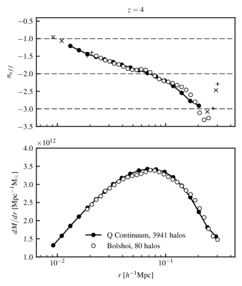
To illustrate the closeness of obtained profiles across simulations, we compare our results with Klypin et al. (2011) and Prada et al. (2012) who calculate the concentrations of halos from the MultiDark and Bolshoi project suite of simulations. These halo profiles are publicly available in the CosmoSim database333https://www.cosmosim.org/cms/simulations. The cosmologies of the Bolshoi and MultiDark simulations differ from ours, but the mass resolutions of Bolshoi () and Q Continuum () are similar. A stacked profile of high-redshift Bolshoi halos overlaps with a Q Continuum profile at the same mass and redshift (Figure 13); the shape of the halo profiles is essentially the same.
A.2 The – Relation in Other Simulations
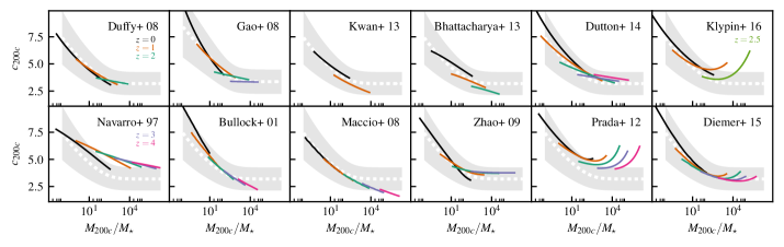
Many different methods have been used to measure concentrations from a large set of simulations. The results fall in one of three categories: concentration is power-law at all masses and redshifts; concentration flattens at high masses and redshifts; or concentration increases at high mass and redshift. Our results are most consistent with the second category; we do not find evidence that concentration increases with mass at high masses and redshifts, but instead find that it approaches a constant . Selected fits and analytical models of all three types are compared to our results in Figure 14. Masses are scaled by and multiple redshifts are shown to check for redshift-independent behavior in others’ results; note, however, that the – relation is not fully cosmology-independent – concentrations are higher in high- cosmologies.
The first papers to note a deviation from power-law behavior at high mass and redshift described a flattening of the – relation. Zhao et al. (2003) describe a concentration floor at and a mass-independent – relation at high redshift; their plot may show a slight upward slope. Neto et al. (2007) provide results only for , but comment on a tendency toward constant concentration at high mass. Gao et al. (2008) note a flattening at high mass and redshift. The model of Zhao et al. (2009), which predicts concentration from the time when a halo reaches a fraction of its final mass, predicts a flat regime at high masses and redshifts; again, the results at may slope slightly upward, but are fit to a model that predicts mass-independent concentration. Two results at high redshift also find very shallow – relations: Hellwing et al. (2016) provide results for relaxed halos only, but find that the – relation flattens at redshifts up to . Angel et al. (2016) find a shallow – relation for relaxed halos at ; the – relation for the full halo sample is shown to be consistent with the upturn of Diemer & Kravtsov (2015), but also appears to be consistent with a flat relation.
Using a new method to measure concentration, based on maximum circular velocity , Klypin et al. (2011) note an upturn in the – relation. The upturn is stronger for relaxed halos (in addition to our criterion that the distance between halo centers fall within , their halos are only relaxed if spin parameter ). The reasons for the upturn are unknown, but the statistics of the highest density peaks are suggested as a possible explanation. Using a modified version of the method and including only bound particles in halo profiles, Prada et al. (2012) also find an upturn. The upturn is also seen in relaxed halos selected using the spin parameter and center-offset criteria as well as an additional requirement that the virial ratio . Elaborating on the statistics of high-density peaks, Prada et al. (2012) show that infall velocity is greatest for the most massive halos. Klypin et al. (2016) returns to this point, suggesting that greater infall velocity will produce more concentrated halos, and notes a relationship between true concentration and the Einasto shape parameter . Muñoz-Cuartas et al. (2011) use a profile fitting method rather than ; power-law fits are used to describe their results, but a flattening of the – relation at high mass is noted to be consistent with Klypin et al. (2011). Correa et al. (2015) fit density profiles, and find an upturn or flattening when all halos are included in the – relation, but not when the sample is restricted to relaxed halos. Diemer & Kravtsov (2015) also use a density profile fitting method, find an upturn, and propose a model that predicts a positive slope for the high- – relation.
The methods of the above papers differ in several respects. Other papers discuss the effects of these differences in methodology on the – relation. Ludlow et al. (2012) find an upturn using the method, but the upturn is not seen when the halo sample is restricted to relaxed halos selected using two criteria (virial ratio and fraction of mass in substructure) in addition to our restriction on the distance between halo centers (the – relation for our unrelaxed halo sample does not differ from that of relaxed halos in shape, only in amplitude). The additional criteria are relevant, as halos are seen to pass through phases of high concentration immediately following major mergers: when the infalling progenitor passes near the center of the halo, the halo is highly concentrated and is classified as unrelaxed according to the virial ratio test. Ludlow et al. (2014), Angel et al. (2016), and Hellwing et al. (2016) also see no upturn in the relaxed-halo – relation. Meneghetti & Rasia (2013) are able to bring the results of Prada et al. (2012) into agreement with those of Duffy et al. (2008) by binning halos in as opposed to , and by measuring concentration through profile fitting as opposed to the method. Dutton & Maccio (2014) do find that the – relation slopes upward at when the method is used, but is flat when concentrations are determined by a profile fit method. The – relations are fit to power laws, but do show either a slight upturn or plateau at high masses and redshifts. Rodriguez-Puebla et al. (2016), however, do find an upturn in concentrations measured by profile fitting as well as using the method; Klypin et al. (2016) find an upturn both when binning in and in virial mass.
A.3 Models of the – Relation
Several different fits and models, with varying levels of physical motivation, have been used to describe the – relation. The simplest description is a power-law fit at each redshift to concentration as a function of mass (top row of Figure 14: Duffy et al. 2008; Gao et al. 2008; Kwan et al. 2013; Dutton & Maccio 2014). In the case of the upturn, a third parameter is needed to fit , as in Klypin et al. (2016). The peak-height parameter has been used as the independent parameter to find a redshift-independent – relation; the shape may simply be fit, as in e.g. Bhattacharya et al. (2013), or described by a model (bottom row of Figure 14).
One set of models assumes that the density of the central regions of a halo is determined by the background density at the time the halo forms. The model of Navarro, Frenk, & White (1997) predicts the concentration of a halo of mass from the collapse redshift , the redshift when the total mass of progenitors of mass () or greater first reaches , calculated using the extended Press–Schechter formalism. Concentration is found by assuming that the mean density at determines the density of the final halo within . The model is found to describe simulated – relations for small values of . Bullock et al. (2001) revise the model of Navarro, Frenk, & White (1997); the collapse redshift is found as the time when the collapse mass, , first reaches a fraction of the final halo mass, . In addition to the free parameter, , a second parameter, , relates a density of the halo to the background density at . Macciò et al. (2008) modify the Bullock et al. (2001) model, allowing the halo overdensity with respect to the mean background density to change with redshift.
Using mass accretion histories, Zhao et al. (2009) find that concentration of a halo of mass can be calculated from the age of the universe, , when its main progenitor first reached a mass of . This time is calculated from a model of mass accretion history. The fit to concentration as a function of and predicts a constant concentration of when . Combined with the mass accretion histories, this implies a flat – relation at high redshift, where halos rapidly accrete mass; by , a halo of mass is approaching the stage of its evolution where concentration begins to grow. This model is also used by van den Bosch (2014), with modified parameters, to describe concentrations found using the maximum circular velocity method of Klypin et al. (2011). Wechsler et al. (2002) and Zhao et al. (2003) also provide concentrations based on mass accretion history fits. Correa et al. (2015) combine mass accretion histories, extended Press–Schechter theory, and a fit relationship between concentration and formation time, defined as the time the mass of a halo’s main progenitor reaches the mass within the scale radius of the descendant halo. This model predicts concentration that falls with mass for relaxed halos at all masses and redshifts.
Two other models use an additional cosmology-dependent variable to fit the – relation. Prada et al. (2012) describe concentration as a function of and a time variable , motivated by its appearance in the growth factor . Diemer & Kravtsov (2015) develop a model in which concentration is a function of both and the local slope of the power spectrum, .
Two papers that predict halo concentrations from the initial Gaussian random field are consistent with our results. Dalal et al. (2010) predict halo profiles from the shapes of initial peaks in the Gaussian random field, then fit those profiles to an NFW form to find the concentration. The shape of the – relation is determined by the outer slopes of these peaks. For high-mass halos, where slope is shallow and consistent with a prediction from Gaussian statistics, concentration is independent of halo mass. The outer slopes of simulated peaks corresponding to low-mass halos differ from the Gaussian statistics predictions and produce halo profiles with higher concentrations. The transition between these two regimes is redshift-dependent, but falls between and for . Okoli & Afshordi (2016) calculate the initial energy of a region before collapse, then assume energy is conserved and use the Jeans equation to find concentration from the final energy. In the case of spherical collapse (valid for the largest halos), the resulting concentration is mass-independent. For smaller halos, ellipsoidal collapse predicts concentrations that fall with mass.
A.4 Gaussian Distribution of Concentrations
As discussed in Section 3.1 above, we find that concentrations within a mass bin are normally distributed. Reed et al. (2011) and Bhattacharya et al. (2013) also discuss the Gaussian distribution of their concentration measurements. Figure 15 compares our results in corresponding mass bins. There is very good agreement, in the lowest mass bin, with the results of Bhattacharya et al. (2013); the corresponding simulations have very similar mass resolutions. The two higher mass bins of Bhattacharya et al. (2013) use a simulation with significantly worse mass resolution, which may explain the worse agreement with our results. The agreement with Reed et al. (2011) is very interesting, considering that the underlying cosmology differs considerably from the one used here. We note that the mass bin here is by no means narrow; our – relation falls by 25% from the lowest mass in this mass bin to the highest.

A.5 Peak Height Parameter
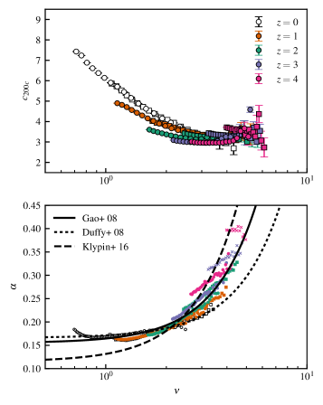
Efforts to find a redshift-independent expression for profile parameters often (e.g. Gao et al. 2008; Prada et al. 2012; Dutton & Maccio 2014; Klypin et al. 2016) convert mass to the “peak height” parameter . Like , is defined from the mean square perturbation (Equation 16):
| (A1) |
We again use . Note that , but is much less sensitive to mass and redshift than . In Figure 16, we see disagreement between concentrations at different redshifts at low . Figure 10 shows that scaling mass by does not suggest a redshift-independent scaling for the Einasto shape parameter, but we do not find significant improvement when is expressed as a function of . The relation is too flat at high to fall on the same line as the lower- relations, as seen in Figure 16. However, our results are in reasonable agreement with those of Gao et al. (2008) for , (and slightly less so with the Planck cosmology results of Klypin et al. 2016). A discrepancy with the model of Gao et al. (2008) arises at , but the model was developed using results only at .
Appendix B Sources of Error
Characteristics of the simulation, such as timestep or initial redshift, or of the halo finder, such as the choice of halo center, may affect the shape or amplitude of the – relation. We check some of the error scenarios in small simulations, and others using the different properties of the Q Continuum and Outer Rim simulations. We find that the – relation as obtained here is robust for . However, there is more distortion at higher redshifts, where, as expected, the agreement between our two simulations with different mass resolutions deteriorates. Below, we present our tests and comment on the various results obtained.
Unfortunately, none of these tests are able to reproduce the differently shaped – relations found by other works in Appendix A.2 above. No two works use the same procedures, so the many remaining methodological differences we are unable to test must contribute to the discrepancies between the resulting – relations. These include halo identification algorithms, the exclusion of unbound particles from halo profiles, and methods of calculating concentrations, among others.
B.1 Initial Redshift
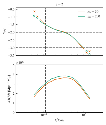
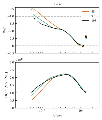
The large simulations are initialized at . (In general, the simulations follow the guidelines laid down in Heitmann et al. 2010.) We compare a small simulation (same cosmology with box size and ) with this initial redshift to one with a deliberately extreme value of . While differences in the profiles are visible at , the – relations differ by only a few percent. The two small simulations have the same seed, so halos form at the same locations; two halos with the same center are the same halo and can be directly compared. At , 35,551 halos of at least 2000 particles are found in the simulation with ; 28,874 are found in the simulation with . More halos form in the simulation with higher initial redshift, so we select relaxed halos from and pair each with the halo whose center is closest, then stack in narrow mass bins. As seen in the stacked profile of Figure 17, the halos lose mass at all radii (more than 90% of the halos have higher mass than their pairs), while the slope of the profile is unchanged. In particular, note that the radius at which is identical; the small change in mass, thus , does produce a slightly higher concentration when . For the example in Figure 17, increases from when to when .
B.2 Timesteps
In this test, we run smaller simulations (same cosmology with box size and same mass resolution as Q Continuum, ) with half, twice, and the same number of timesteps as for the larger simulations. Again, all three test simulations use the same seed, so the profiles of paired halos can be compared. At , 2782 halos of at least 2000 particles are found in the simulation with the standard number of timesteps; 2625 are found in the simulation with halved timesteps, and 2705 when timesteps are doubled. The fewest halos form with halved timesteps, so relaxed halos are selected from that simulation and paired with the closest halos in the others. As shown in Figure 18, the profile at large radius is unchanged, but the inner profile requires more timesteps to converge. Note that all three profiles cross and peak at the same point, indicating no change in scale radius. The shape of the – relation is essentially unaffected; at , doubling the number of timesteps shifts the – relation uniformly up by less than 5% for both fit and accumulated mass methods, while halving timesteps shifts it down by about 8%.
B.3 Halo Centering
We identify the center of a halo as the most bound particle (MBP), locating the local minimum of the potential. Other methods select the most connected particle (MCP, the particle with the greatest number of FOF neighbors), or use a histogram method to find the maximum density. We compare these three methods for a test simulation at . For relaxed halos, where the MBP and MCP centers can differ by , the concentrations vary by less than 5%. The distance between centers is greater for unrelaxed halos – an average of . At low masses, their fit concentrations differ as well; MCP and histogram fit concentrations are up to 20% greater than MBP for halos of 2000 particles, , while the difference returns to less than 5% at high masses.
B.4 Inner Profile
As seen in Figures 8 and 18, differences from the ‘true’ profile are more pronounced in the inner profile than at large radius. Error in the inner profile may have little effect on measurements of NFW concentration, but the Einasto profiles are more sensitive to profile shape; a small change in the inner profile produces a larger change in the shape parameter than in the concentration, as seen in Figures 10 and 19. Inner-profile discrepancies between Outer Rim and Q Continuum arise only at high redshift; where measurements of the shape parameter are inconsistent, the higher-resolution Q Continuum profiles are closer to the ‘true’ shape. The convergence in the inner profile is consistent with the considerations presented in Power et al. (2003).
B.5 Peak-finding Method
We present only for lower-concentration halos; this is because of a systematic error that can arise due to insufficient mass resolution. Figure 20 shows the artificially high measurements found at lower masses at : when concentration is high, is found at smaller radii, where error in particle counts per radial bin may be substantial. For a low-mass Outer Rim halo at with mass and concentration , is found around . A single radial bin at this radius will contain about 100 particles; even with three-point smoothing, the peak is noisy. The other two methods are less susceptible to this error: accumulated mass sums over neighboring bins, and profile fit takes the Poisson error in each bin into account. At high masses and low concentrations, however, the relevant radial bins contain 1–2 orders of magnitude more particles; the peak is better defined and the peak-finding method finds concentrations more similar to the results of the other methods.
B.6 Minimum Particle Count
We present concentrations only for halos of at least 2000 particles, as in Bhattacharya et al. (2013). Neto et al. (2007) discuss conservative minimum particle counts of to ensure high-quality fits and agreement between different mass resolutions. Poveda-Ruiz et al. (2016), finding statistical bias in concentration measurements of halos resolved with hundreds of particles, advocate a minimum particle count of approximately 4000 particles. Because the mass resolutions of Outer Rim and Q Continuum differ by a factor of 20, the two simulations can be used to check for convergence at fixed mass. (The concentrations of 100-particle Outer Rim halos, for example, can be compared to 2000-particle Q Continuum halos of the same mass.) As seen in Figure 20, 2000 particles is sufficient for fit and accumulated mass methods to agree, but, as discussed above, the peak method can be used safely only on larger, less concentrated halos.
References
- Amodeo et al. (2016) Amodeo, S., Ettori, S., Capasso, R., & Sereno, M. 2016, A&A, 590, A126
- Angel et al. (2016) Angel, P.W., Poole, G.B., Ludlow, A.D., Duffy, A.R., Geil, P.M., Mutch, S.J., Mesinger, A., & Wyithe, J.S.B. 2016, MNRAS, 459, 2106
- Baugh (2006) Baugh, C.M. 2006, RPPh., 69, 3101
- Benson (2010) Benson, A.J. 2010, PhR, 495, 33
- Benson et al. (2003) Benson, A.J., Bower, R.G., Frenk, C.S., Lacey, C.G., Baugh, C.M., & Cole, S. 2003, ApJ, 599, 38
- Benson et al. (2000) Benson, A.J., Cole, S., Frenk, C.S., Baugh, C.M., & Lacey, C.G. 2000, MNRAS, 311,793
- Berlind & Weinberg (2002) Berlind, A.A. & Weinberg, D.H. 2002, ApJ, 575, 587
- Bhattacharya et al. (2013) Bhattacharya, S., Habib, S., Heitmann, K., & Vikhlinin, A. 2013, ApJ 766, 32
- Bhattacharya et al. (2011) Bhattacharya, S., Heitmann, K., White, M., Lukić, Z., Wagner, C., & Habib, S. 2011, ApJ, 732, 211
- Brimioulle et al. (2013) Brimioulle, F., Seitz, S., Lerchster, M., Bender, R., & Snigula, J. 2013, MNRAS 432, 1046
- Broadhurst et al. (2008) Broadhurst, T., Umetsu, K., Medezinski, E., Oguri, M., & Rephaeli, Y. 2008, ApJL, 685, L9
- Bullock et al. (2001) Bullock, J.S., Kolatt, T.S., Sigad, Y., Somerville, R.S., Kravtsov, A.V., Klypin, A.A., Primack, J.R., & Dekel, A. 2001, MNRAS, 321, 559
- Cibirka et al. (2017) Cibirka, N., Cypriano, E.S., Brimioulle, F., Gruen, D., Erben, T., van Waerbeke, L., Miller, L., Finoguenov, A., Kirkpatrick, C., Henry, J.P., Rykoff, E., Rozo, E., Dupke, R., Kneib, J-P., Shan, H., & Spinelli, P. 2017, MNRAS, 468, 1092
- Cole et al. (1994) Cole, S., Aragon-Salamanca, A., Frenk, C.S., Navarro, J.F., & Zepf, S.E. 1994, MNRAS 271, 781
- Comerford & Natarajan (2007) Comerford, J.M. & Natarajan, P. 2007, MNRAS, 379, 190
- Conroy et al. (2006) Conroy, C., Wechsler, R.H., & Kravtsov, A.V. 2006, ApJ, 647, 201
- Correa et al. (2015) Correa, C.A., Wyithe, J.S.B., Schaye, J., & Duffy, A. 2015, MNRAS, 452, 1217
- Dalal et al. (2010) Dalal, N., Lithwick, Y., & Kuhlen, M. 2010, arXiv:1010.2539
- Diemer & Kravtsov (2015) Diemer, B., & Kravtsov, A.V. 2015, ApJ, 799, 108
- Dolag et al. (2004) Dolag, K., Bartelmann, M., Perrotta, F., Baccigalupi, C., Moscardini, L. Meneghetti, M. & Tormen, G. 2004, A&A, 416, 853
- Duffy et al. (2010) Duffy A.R., Schaye, J., Kay, S.T., Dalla Vecchia, C., Battye, R.A., & Booth, C.M. 2010, MNRAS, 405, 2161
- Duffy et al. (2008) Duffy, A.R., Schaye, J., Kay, S.T., & Dalla Vecchia, C. 2008, MNRAS, 390, L64
- Dutton & Maccio (2014) Dutton, A.A. & Macciò, A.V. 2014, MNRAS, 441, 3359
- Einasto (1965) Einasto, J. 1965, Trudy Astrofizicheskogo Instituta Alma-Ata, 5, 87
- Eke et al. (2001) Eke, V., Navarro, H., & Steinmetz, M. 2001, ApJ, 554, 115
- Foëx et al. (2014) Foëx, G., Motta, V., Jullo, E., Limousin, M., & Verdugo, T. 2014, A&A 572, A19
- Gao et al. (2008) Gao, L., Navarro, J.F., Cole, S., Frenk, C.S., White, S.D.M., Springel, V., Jenkins, A., & Neto, A.F. 2008, MNRAS, 387, 536
- Gil-Marín et al. (2018) Gil-Marín, H., Guy, J., Zarrouk, P., Burtin, E., Chuang, C.-H., Percival, W.J., Ross, A.J., Ruggeri, R., Tojerio, R., Zhao, G.-B., Wang, Y., Bautista, J., Hou, J., Sánchez, A.G., Pâris, I., Baumgarten, F., Brownstein, J.R., Dawson, K.S., Eftekharzadeh, S., Gonz lez-P rez, V., Habib, S., Heitmann, K., Myers, A.D., Rossi, G., Schneider, D.P., Tinker, J.L., & Zhao, C. 2018, arXiv:1801.02689
- Guo et al. (2010) Guo, Q., White, S., Cheng, L., & Bolyan-Kolchin, M. 2010, MNRAS, 404, 1111
- Habib et al. (2016) Habib, S., Pope, A., Finkel, H., Frontiere, N., Heitmann, K., Daniel, D., Fasel, P., Morozov, V., Zagaris, G., Peterka, T., Vishwanath, V., Lukić, Z., Sehrish, S., & Liao, W.K. 2016, NewA, 42, 49
- Hearin et al. (2016) Hearin, A.P., Zentner, A.R., van den Bosch, F.C., Campbell, D., & Tollerud, E. 2016, MNRAS, 460, 2552
- Heitmann et al. (2016) Heitmann, K., Bingham, D., Lawrence, E., Bergner, S., Habib, S., Higdon, D., Pope, A., Biswas, R., Finkel, H., Frontiere, N., & Bhattacharya, S. 2016, ApJ, 820, 108
- Heitmann et al. (2014) Heitmann, K., Frontiere, N., Sewell, C., Habib, S., Pope, A., Finkel, H., Rizzi, S., Insley, J., & Bhattacharya, S. 2015, ApJS, 219, 34
- Heitmann et al. (2006) Heitmann, K., Lukić, Z., Habib, S., Ricker, P.M. 2006, ApJL, 642, L85
- Heitmann et al. (2010) Heitmann, K., White, M., Wagner, C., Habib, S., & Higdon, D. 2010, ApJ, 715, 104
- Hellwing et al. (2016) Hellwing, W.A., Frenk, C.S., Cautun, M., Bose, S., Helly, J., Jenkins, A., Sawala, T., & Cytowski, M. 2015, MNRAS, 457, 3492
- Holder et al. (2001) Holder, G., Haiman, Z., & Mohr, J.J. 2001, ApJL, 560, L111
- Hou et al. (2018) Hou, J., Sánchez, A.G., Scoccimarro, R., Salazar-Albornoz, S., Burtin, E., Gil-Marín, H., Percival, W.J., Ruggeri, R., Zarrouk, P., Zhao, G.-B., Bautista, J., Brinkmann, J., Brownstein, J.R., Dawson, K.S., Devi, N.C., Myers, A.D., Habib, S., Heitmann, K., Tojeiro, R., Rossi, G., Schneider, D.P., Seo, H.-J., & Wang, Y. 2018, arXiv:1801.02656
- Hu & Kravtsov (2003) Hu, W. & Kratsov, A.V. 2003, ApJ, 584, 702
- Jenkins et al. (2001) Jenkins, A., Frenk, C.S., White, S.D.M., Colberg, J.M., Cole, S., Evrard, A.E., Couchman, H.M.P., & Yoshida, N. 2001, MNRAS, 321, 372
- Jing et al. (1998) Jing, Y.P., Mo, H.J., & Börner, G. 1998, ApJ, 494, 1
- Jing & Suto (2002) Jing, Y.P., & Suto, Y. 2002, ApJ, 574, 538
- Johnston et al. (2007) Johnston, D.E., Sheldon, E.S., Wechsler, R.H., Rozo, E., Koester, B.P., Frieman, J.A., McKay, T.A., Evrard, A.E., Becker, M.R., & Annis, J. 2007, arXiv:0709.1159
- Kauffmann et al. (1997) Kauffmann, G., Nusser, A., & Steinmetz, M. 1997, MNRAS, 286, 795
- Kauffmann et al. (1993) Kauffmann, G., White, S.D.M., & Guiderdoni, B. 1993, MNRAS, 264, 201
- Klypin et al. (2016) Klypin, A., Yepes, G., Göttlober, S., Prada, F., & Heß, S. 2016, MNRAS, 457, 4340
- Klypin et al. (2011) Klypin, A.A., Trujillo-Gomez, S., & Primack, J. 2011, ApJ, 740, 102
- Komatsu et al. (2011) Komatsu, E., Smith, K.M., Dunkley, J., Bennett, C.L., Gold, B., Hinshaw, G., Jarosik, N., Larson, D., Nolta, M.R., Page, L., Spergel, D.N., Halpern, M., Hill, R.S., Kogut, A., Limon, M., Meyer, S.S., Odegard, N., Tucker, G.S., Weiland, J.L., Wollack, E., & Wright, E.L. 2011, ApJS, 192, 18
- Kwan et al. (2013) Kwan, J., Bhattacharya, S., Heitmann, K., & Habib, S. 2013, ApJ, 768, 123
- Lawrence et al. (2017) Lawrence, E., Heitmann, K., Kwan, J., Upadhye, A., Bingham, D., Habib, S., Higdon, D., Pope, A., Finkel, H., & Frontiere, N. 2017, arXiv:1705.03388
- Lewis et al. (2000) Lewis, A., Challinor, A., & Lasenby, A. 2000, ApJ, 538, 473
- LSST Science Collaboration et al. (2009) LSST Science Collaboration, Abell, P.A., Allison, J., et al. 2009, arXiv:0912.0201
- Ludlow et al. (2016) Ludlow, A.D., Bose, S., Angulo, R.E., Wang, L., Hellwing, W.A., Navarro, J.F., Cole, S., & Frenk, C.S. 2016, MNRAS, 460, 1214
- Ludlow et al. (2014) Ludlow, A.D., Navarro, J.F., Angulo, R.E., Boylan-Kolchin, M., Springel, V., Frenk, C., & White, S.D.M. 2014, MNRAS, 441, 378
- Ludlow et al. (2012) Ludlow, A.D., Navarro, J.F., Li, M., Angulo, R.E., Boylan-Kolchin, M., & Bett, P.E. 2012, MNRAS, 427, 1322
- Lukić et al. (2007) Lukić, Z., Heitmann, K., Habib, S., Bashinsky, S., & Ricker, P.M. 2007, ApJ, 671, 1160
- Lukić et al. (2009) Lukić, Z., Reed, D., Habib, S., & Heitmann, K. 2009, 692, 217
- Macciò et al. (2008) Macciò, A.V., Dutton, A.A., & van den Bosch, F.C. 2008, MNRAS, 391, 1940
- Mandelbaum et al. (2006) Mandelbaum, R., Seljak, U., Cool, R.J., Blanton, M., Hirata, C.M., & Brinkmann, J. 2006, MNRAS, 372, 758
- Mandelbaum et al. (2008) Mandelbaum, R., Seljak, U., & Hirata, C.M. 2008, JCAP 0808, 006
- Meneghetti et al. (2005) Meneghetti, M., Bartelmann, M., Dolag, K., Moscardini, L., Perrotta, F., Baccigalupi, C., & Tormen, G. 2005, A&A, 442, 413
- Meneghetti & Rasia (2013) Meneghetti, M. & Rasia, E. 2013, arXiv:1303.6158
- Merritt et al. (2006) Merritt, D., Graham, A.W., Moore, B., Diemand, J. & Terzić, B. 2006, AJ, 132, 2685
- Merten et al. (2015) Merten, J., Meneghetti, M., Postman, M., Umetsu, K., Zitrin, A., Medezinski, E., Nonino, M., Koekemoer, A., Melchior, P., Gruen, D., Moustakas, L.A., Bartelmann, M., Host, O., Donahue, M., Coe, D., Molino, A., Jouvel, S., Monna, A., Seitz, S., Czakon, N., Lemze, D., Sayers, J., Balestra, I., Rosati, P., Benítez, N., Biviano, A., Bouwens, R., Bradley, L., Broadhurst, T., Carrasco, M., Ford, H., Grillo, C., Infante, L., Kelson, D., Lahav, O., Massey, R., Moustakas, J., Rasia, E., Rhodes, J., Vega, J., & Zheng, W. 2015, ApJ, 806, 4
- Moster et al. (2010) Moster, B.P., Somerville, R.S., Maulbetsch, C., van den Bosch, F.C., Maccio, A.V., Naab, T., & Oser, L. 2010, ApJ, 710, 903
- Muñoz-Cuartas et al. (2011) Muñoz-Cuartas, J.C., Macciò, A.V., Gottlöber, S., & Dutton, A.A. 2011, MNRAS, 411, 584
- Navarro, Frenk, & White (1996) Navarro, J.F., Frenk, C.S., & White, S.D.M. 1996, ApJ, 462, 563
- Navarro, Frenk, & White (1997) Navarro, J.F., Frenk, C.S., & White, S.D.M. 1997, ApJ, 490, 493
- Navarro et al. (2004) Navarro, J.F., Hayashi, E., Power, C., Jenkins, A.R., Frenk, C.S., White, S.D.M., Springel, V., Stadel, J. & Quinn, T.R. 2004, MNRAS, 349, 1039
- Neto et al. (2007) Neto, A.F., Gao, L., Bett, P., Cole, S., Navarro, J.F., Frenk, C.S., White, S.D.M., Springel, V., & Jenkins, A. 2007, MNRAS, 381, 1450
- Newman et al. (2013) Newman, A.B., Treu, T., Ellis, R.S., Sand, D.J., Nipoti, C., Richard, J., & Jullo, E. 2013, ApJ, 765, 24
- Niikura et al. (2015) Niikura, H., Takada, M., Okabe, N., Martino, R., & Takahashi, R. 2015, PASJ, 67, 103
- Oguri et al. (2012) Oguri, M., Bayliss, M.B., Dahle, H., Sharon, K, Gladders, M.D., Natarajan, P., Hennawi, J.F., & Koester, B.P. 2012, MNRAS, 420, 3213
- Okabe & Smith (2016) Okabe, N. & Smith, G.P. 2016, MNRAS, 461, 2794
- Okabe et al. (2013) Okabe, N., Smith, G.P., Umetsu, K., Takada, M., & Futamase, T. 2013, ApJL, 769, L35
- Okabe et al. (2010) Okabe, N., Takada, M., Umetsu, K., Futamase, T., & Smith, G.P. 2010, PASJ, 62, 811
- Okoli & Afshordi (2016) Okoli, C. & Afshordi, N. 2016, MNRAS, 456, 3068
- Peacock & Smith (2000) Peacock, J.P. & Smith, R.E. 2000, MNRAS, 318, 1144
- Poveda-Ruiz et al. (2016) Poveda-Ruiz, C.N., Forero-Romero, J.E., & Muñoz-Cuartas, J.C. 2016, ApJ, 832, 169
- Power et al. (2003) Power, C., Navarro, J.F., Jenkins, A., Frenk, C.S., White, S.D.M., Springel, V., Stadel, J. & Quinn, T. 2003, MNRAS, 338, 14
- Prada et al. (2012) Prada, F., Klypin, A.A., Cuesta, A.J., Betancort-Rijo, J.E., & Primack, J. 2012, MNRAS, 423, 3018
- Prada et al. (2006) Prada, F., Klypin, A.A., Simonneau, E., Betancort-Rijo, J., Patiri, S., Gottlöber, S. & Sanchez-Conde, M.A. 2006, ApJ, 645, 1001
- Reed et al. (2011) Reed, D.S., Koushiappas, S.M., & Gao, L. 2011, MNRAS, 415, 3177.
- Refregier et al. (2010) Refregier, A., Amara, A., Kitching, T.D., Rassat, A., Scaramella, R., & Weller, J. 2010, arXiv:1001.0061 [astro-ph.IM]
- Rodriguez-Puebla et al. (2016) Rodríguez-Puebla, A., Behroozi, P., Primack, J., Klypin, A., Lee, C., & Hellinger, D. 2016, MNRAS, 462, 893
- Schmidt & Allen (2007) Schmidt, R.W., & Allen, S.W. 2007, MNRAS, 379, 209
- Seljak (2000) Seljak, U. 2000, MNRAS, 318, 203
- Sereno & Covone (2013) Sereno, M. & Covone, G. 2013, MNRAS, 434, 878
- Simet et al. (2017) Simet, M., McClintock, T., Mandelbaum, R., Rozo, E., Rykoff, E., Sheldon, E., & Wechsler, R.H. 2017, MNRAS, 466, 3103
- Somerville & Primack (1999) Somerville, R.S. & Primack, J.R. 1999, MNRAS, 310, 1087
- Spergel et al. (2015) Spergel, D., Gehrels, N., Baltay, C., Bennett, D., Breckinridge, J., Donahue, M., Dressler, A., Gaudi, B.S., Greene, T., Guyon, O., Hirata, C., Kalirai, J., Kasdin, N.J., Macintosh, B., Moos, W., Perlmutter, S., Postman, M., Rauscher, B., Rhodes, J., Wang, Y., Weinberg, D., Benford, D., Hudson, M., Jeong, W.-S., Mellier, Y., Traub, W., Yamada, T., Capak, P., Colbert, J., Masters, D., Penny, M., Savransky, D., Stern, D., Zimmerman, N., Barry, R., Bartusek, L., Carpenter, K., Cheng, E., Content, D., Dekens, F., Demers, R., Grady, K., Jackson, C., Kuan, G., Kruk, J., Melton, M., Nemati, B., Parvin, B., Poberezhskiy, I., Peddie, C., Ruffa, J., Wallace, J.K., Whipple, A., Wollack, E., & Zhao, F. 2015, arXiv:1503.03757 [astro-ph.IM]
- Umetsu et al. (2011) Umetsu, K., Broadhurst, T., Zitrin, A., Medezinski, E., & Postman, M. 2011, ApJ, 738, 41
- Umetsu & Diemer (2017) Umetsu, K. & Diemer, B. 2017, ApJ, 836, 231
- Umetsu et al. (2014) Umetsu, K., Medezinski, E., Nonino, M., Merten, J., Postman, M., Meneghetti, M., Donahue, M., Czakon, N., Molino, A., Seitz, S., Gruen, D., Lemze, D., Balestra, I., Benítez, N., Biviano, A., Broadhurst, T., Ford, H., Grillo, C., Koekemoer, A., Melchior, P., Mercurio, A., Moustakas, J., Rosati, P., & Zitrin, A. 2014, ApJ, 795, 163
- Umetsu et al. (2016) Umetsu, K., Zitrin, A., Gruen, D., Merten, J., Donahue, M., & Postman, M. 2016, ApJ, 821, 116
- Vale & Ostriker (2004) Vale, A. & Ostriker, J.P. 2004, MNRAS, 353, 189
- van den Bosch (2014) van den Bosch, F.C., Jiang, F., Hearin, A., Campbell, D., Watson, D., & Padmanabhan, N. 2014, MNRAS, 445, 1713
- Vikhlinin et al. (2006) Vikhlinin, A., Kravtsov, A., Forman, W., Jones, C., Markevitch, M., Murray, S.S., & Van Speybroeck, L. 2006, ApJ, 640, 691
- Wechsler et al. (2002) Wechsler, R.H., Bullock, J.S., Primack, J.R., Kravtsov, A.V., & Dekel, A. 2002, ApJ, 568, 52
- Wetzel & White (2010) Wetzel, A.R. & White, M. 2010, MNRAS, 403, 1072
- White (2002) White, M. 2002, ApJS, 143, 241
- White & Frenk (1991) White, S.D.M. & Frenk, C.S. 1991, ApJ, 379, 52
- Zarrouk et al. (2018) Zarrouk, P., Burtin, E., Gil-Marín, H., Ross, A.J., Tojeiro, R., Pâris, I., Dawson, K.S., Myers, A.D., Percival, W.J., Chuang, C.-H., Zhao, G.-B., Bautista, J., Comparat, J., González-Pérez, V., Habib, S., Heitmann, K., Hou, J., Laurent, P., Le Goff, J.-M., Prada, F., Rodríguez-Torres, S.A., Rossi, G., Ruggeri, R., Sánchez, A.G., Schneider, D.P., Tinker, J.L., Wang, Y., Yèche, C., Baumgarten, F., Brownstein, J.R., de la Torre, S., du Mas des Bourboux, H., Kneib, J.-P., Palanque-Delabrouille, N., Peacock, J., Petitjean, P., Seo, H.-J., & Zhao, C. 2018, arXiv:1801.03062
- Zhao et al. (2003) Zhao, D.H., Jing, Y.P., Mo, H.J., & Börner, G. 2003, ApJL, 597, L9
- Zhao et al. (2009) Zhao, D.H., Jing, Y.P., Mo, H.J., & Börner, G. 2009, ApJ, 707, 354
- Zheng et al. (2005) Zheng, Z., Berlind, A.A., Weinberg, D.H., Benson, A.J., Baugh, C.M., Cole, S., Davé, R., Frenk, C.S., Katz, N., & Lacey, C.G. 2005, ApJ 633, 791