Shape of a skyrmion

Abstract

We propose a method of determining the shape of a two-dimensional magnetic skyrmion, which can be parameterized as the position dependence of the orientation of the local magnetic moment, by using the expansion in terms of the eigenfunctions of the Schrödinger equation of a harmonic oscillator. A variational calculation is done, up to the next-to-next-to-leading order. This result is verified by a lattice simulation based on Landau-Lifshitz-Gilbert equation. Our method is also applied to the dissipative matrix in the Thiele equation as well as two interacting skyrmions in a bilayer system.

I Introduction

A magnetic skyrmion is a two-dimensional (2D) topologically protected swirling spin texture in a chiral magnet nagaosa ; Fert . It was discovered in an intermetallic compound MnSi by using neutron scattering Muhlbauer , and was also observed by using Lorentz transmission electron microscopy (LTEM) Yu1 , spin-resolved scanning tunnelling microscopy  2DSkyrmion2 , etc. The critical current density for the manipulation of a magnetic skyrmion is much lower than that for magnetic domain walls ultralow . Therefore it was proposed that skyrmions may act as future information carriers in magnetic information storage and processing devices.

For a typical 2D skyrmion, The orientation ${\bf n}$ of the local magnetic moment can be parameterized in cylindrical coordinates as NParameterAndLinear ; NParameterArcTan

$$\begin{split}&{\bf n}(\rho,\phi,z)=\sin[\theta(\rho)]{\bf e}_{\phi}+\cos[\theta(\rho)]{\bf e}_{z},\\ \end{split}$$ (1)

where $\theta$ is the angle between ${\bf n}$ and ${\bf e}_{z}$.

$\theta(\rho)$ describes the shape of a skyrmion. On large scales, a skyrmion can be considered as a point-like particle because of its topological nature. However, on scales compatible with or smaller than its radius, the shape of a skyrmion should be taken into account and becomes an interesting subject. For example, the current-driven motion of a skyrmion can be described in terms of the Thiele equation Thiele , which is widely used in studying rotational property ThieleStudy ; ThieleStudyAndJDB , skyrmion Hall effect Jiang , skyrmions in bilayer systems bilayer1 ; bilayer2 ; Zhang2 , etc. The dissipative matrix in the Thiele equation relies on $\theta(\rho)$. Besides, $\theta(\rho)$ is important in studying the interaction between two skyrmions in bilayer systems bilayer2 , because the interaction is significant only when the two skyrmions are close to each other.

Hence it is important to determine $\theta(\rho)$. Previously, $\theta(\rho)$ was obtained by numerical methods pin or was assumed to either be linear in $\rho$ Jiang ; NParameterAndLinear ; thetarho , or satisfy $\theta(\rho)=\arctan\left(\exp\left(-\rho/\Delta\right)\right)$ NParameterArcTan ; arctan . In this paper, instead, we propose an efficient method to analytically calculate $\theta(\rho)$ of a 2D skyrmion stabilized by an external magnetic field. We find an analytical expression of $\theta(\rho)$ and compare it with our numerical result. We also study the radii of the skyrmions by a lattice simulation of the Landau-Lifshitz-Gilbert (LLG) equation. Using the approximation in our analytical method, the dissipative matrix element and the interaction between the skyrmions can be explicitly expressed in terms of the ferromagnetic coupling, the Dzyaloshinskii-Moriya (DM) interaction strength and the magnetic field. Our analytical result is confirmed by our numerical result.

The rest of the paper is organized as the following. Our analytical method is introduced in Sec. II. Our lattice simulation is discussed in Sec. III. The dissipative matrix element and the interaction between two skyrmions are discussed in Sec. IV. A summary is made in Sec. V.

II Harmonic Oscillator Expansion

First we briefly review the equation of $\theta(\rho)$ in Eq. (1), as well as the numerical solution following the method used in pin .

The Hamiltonian can be written in terms of the dimensionless parameters as FreeEnergy

$$\begin{split}&{\mathcal{H}}_{\rm tot}({\bf r})=\frac{J}{2}\nabla{\bf n}\cdot\nabla{\bf n}+D{\bf n}\cdot(\nabla\times{\bf n})-{\bf B}\cdot{\bf n},\\ \end{split}$$ (2)

where ${\bf n}$ is the orientation of the local magnetic moment, given above in Eq. (1), $J$ is the local ferromagnetic exchange strength, $D$ is the local strength of DM interaction, ${\bf B}$ is the external magnetic field. $\theta(\rho)$ can be obtained by minimizing the total energy

$$\begin{split}&F=\int d{\bf r}\mathcal{F}(\bf r)=2\pi\int d\rho\rho\mathcal{F}(\rho),\\ \end{split}$$ (3)

where the energy density $\mathcal{F}$ is pin

$$\begin{split}&\mathcal{F}(\rho)={\mathcal{H}}_{\rm tot}(\rho)-{\mathcal{H}}_{\rm fe}=2J\left[\left(\frac{1}{2}\frac{\partial\theta}{\partial\rho}+\kappa\right)^{2}-\kappa^{2}+\frac{\sin^{2}(\theta)}{4\rho^{2}}+\frac{\kappa\sin(2\theta)}{2\rho}\right]-B(\cos(\theta)-1),\\ \end{split}$$ (4)

with $\kappa\equiv D/2J$, ${\mathcal{H}}_{\rm fe}=-B$. It has been assumed that the magnetic field ${\bf B}=B({\bf r}){\bf e}_{z}$ is along $z$ direction. The Euler-Lagrange equation yields

$$\begin{split}&\frac{\sin(\theta)\cos(\theta)}{\rho}-\theta^{\prime}-\rho\theta^{\prime\prime}-2\frac{D}{J}\sin^{2}(\theta)+\frac{B}{J}\rho\sin(\theta)=0,\end{split}$$ (5)

which can be solved numerically by using the scheme of finite differences pin . In the rest of this paper, the numerical solutions are always obtained by using this method.

The main content of our paper is the following analytical method. A function $f(x)$ well defined in $[0,\infty)$, with $f(0)>0$, $f(\infty)=0$, and $\int_{0}^{\infty}dx|f(x)|^{2}$ being finite, can be expanded in terms of the eigenfunctions of the quantum Hamiltonian of an harmonic oscillator,

$$\begin{split}&\phi_{n,\omega}(x)=\left(\frac{\omega}{\pi}\right)^{\frac{1}{4}}\frac{1}{\sqrt{2^{n}n!}}H_{n}(\sqrt{\omega}x)e^{-\frac{\omega x^{2}}{2}},\\ \end{split}$$ (6)

where $H_{n}(x)$ is the Hermite polynomials. $\phi_{n,\omega}(x)$’s are solutions of

$$\begin{split}&\left(\frac{1}{2}\omega^{2}x^{2}+\frac{1}{2}\frac{d^{2}}{dx^{2}}\right)\phi=E\phi.\end{split}$$ (7)

Therefore $f(x)$ can be expanded as

$$\begin{split}&f(x)=\sum_{n=0}^{\infty}C_{n}\phi_{2n,\omega}(x)\\ \end{split}$$ (8)

with $C_{n}=\int_{0}^{\infty}dxf(x)\phi_{2n,\omega}(x)$.

Previous ansatz functions for $\theta(\rho)$ included the linear functions Jiang ; NParameterAndLinear ; NParameterArcTan ; thetarho , as well as $\tan^{-1}(\exp(-\rho/\Delta))$ arctan ; NParameterArcTan . In Appendix A, these ansatz functions are expanded in terms of harmonic oscillator functions, as examples.

II.1 Leading order (LO) approximation

As the numerical solution is close to a Gaussian function, we assume that the LO wave function, as a Gaussian function, is a good approximation. Thus the coefficients in the expansion $\theta(\rho)=\sum_{n}C_{n}\phi_{2n,\omega}(\rho)$ satisfy $C_{0}\gg C_{i>0}$. Under this assumption, one can use the Rayleigh-Ritz variational method RRMethod to obtain $\omega$ and $C_{n}$’s order by order.

At LO, $\theta(\rho)\approx\theta_{\rm LO}(\rho)=C_{0}\left(\omega/\pi\right)^{1/4}\exp(-\omega\rho^{2}/2)$. To ensure $\theta(0)=\pi$ and $\theta(\infty)=0$, we use $\theta_{\rm LO}(\rho)=\pi\exp(-\omega\rho^{2}/2)$ as a trial solution. To minimize the total energy $F$, $\omega$ should satisfy $dF/d\omega=0$, leading to

$$\begin{split}&\frac{D\pi^{\frac{3}{2}}}{2\omega\sqrt{2\omega}}-\frac{D}{4\omega}\int_{0}^{\infty}d\rho\sin(2\pi e^{-\frac{\omega\rho^{2}}{2}})-\frac{B}{2\omega^{2}}\left(2(-\text{Ci}(\pi)+\gamma_{E}+\log(\pi))\right)=0,\end{split}$$ (9)

where $\gamma_{E}$ is the Euler constant, ${\rm Ci}$ is the cosine integral function defined as

$$\begin{split}&{\rm Ci}(z)\equiv-\int_{z}^{\infty}dt\frac{\cos(t)}{t}.\end{split}$$ (10)

The solution can be obtained as

$$\begin{split}&\omega_{\rm LO}=\left(\frac{\sqrt{2}B\left(2(-\text{Ci}(\pi)+\gamma+\log(\pi))\right)}{D(\pi^{\frac{3}{2}}-a_{0})}\right)^{2},\\ \end{split}$$ (11)

where

$$\begin{split}&a_{0}\equiv\frac{1}{\sqrt{2}}\int_{0}^{\infty}dx\sin(2\pi e^{-\frac{x^{2}}{2}})\approx 0.250432,\\ \end{split}$$ (12)

$$\begin{split}&\omega_{\rm LO}\approx 0.768548\left(\frac{B}{D}\right)^{2}.\\ \end{split}$$ (13)

To verify the leading order approximation, some examples of the results from $\theta_{\rm LO}(\rho)$ together with the numerical results are shown in Fig. 1. The parameter values $D/J=0.2$ and $D/B=10$ or $20$ are close to $D/J=0.18$ and $B/J=0.0075$ to $0.0252$ in Ref. ThieleStudyAndJDB . The parameter values $D/J=0.1$ and $D/B=20$ are close to $D/J=0.09$ and $B/J=0.001875$ to $0.0063$ in Ref. JDBRef1 . The parameter values $D/J=0.5$ and $D/B=3$ are close to $D/J=0.5$ and $B/J=0.15-0.3$ in Ref. JDBRef2 .

We also find numerically that for a given value of $D/J$, the size of the skyrmion is nearly independent of $J$, and depends on $D/B$. This is in consistency with the LO approximation, in which $\theta_{\rm LO}(\rho)$ is Gaussian function, thus the radius of a skyrmion is $R\propto\left(\omega_{\rm LO}\right)^{-1/2}\propto D/B$, which is independent of $J$. This is also in consistency with the previous results using dimensionless parameters ThieleStudyAndJDB ; JDBRef1 ; alpha3 ; bilayer2 ; pin ; Tchoe . Note that $J$ is merely an energy unit, and that $\rho$ is also dimensionless. For realistic materials, the radii of the skyrmions depend on realistic ferromagnetic coupling because the unit of $\rho$ depends on it, and the rescaling of $\rho$ must be taken into account. The relation between the dimensionless parameters and the realistic parameters will be discussed in Sec. III.

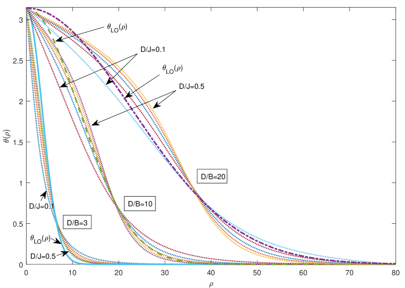
Figure 1: The numerical result of $\theta(\rho)$ and the function $\theta_{\rm LO}(\rho)$. The solid line represents $\theta_{\rm LO}(\rho)$ for $D/B=3$, the dashed line in the middle represents $\theta_{\rm LO}(\rho)$ for $D/B=10$, while the dotted dashed line on the right represents $\theta_{\rm LO}(\rho)$ for $D/B=20$. Around each line of $\theta_{\rm LO}(\rho)$, the five dotted lines represent the numerical results for the corresponding value of $D/B$ and for $D/J=0.1,0.2,0.3,0.4,0.5$. For each group of five dotted lines with a same value of $D/B$, the slope increases with $D/J$.

II.2 Next-to-next-to-leading order (NNLO) approximation

At the next-to-leading order (NLO), the function $\theta(\rho)$ can be approximated as $\theta_{\rm NLO}(\rho)=\pi\exp\left(-\omega\rho^{2}/2\right)+c\pi\omega\rho^{2}\exp\left(-\omega\rho^{2}/2\right)$, where $c$ is a parameter. Solving the equations $dF/d\omega=0$ and $dF/dc=0$, we find that the result is the same as the LO, that is, $c\approx 0$. So we need to consider the NNLO approximation. The trial solution at NNLO can be written as $\theta_{\rm NNLO}(\rho)=C_{0}\phi_{0,\omega}+C_{1}\phi_{2,\omega}+C_{2}\phi_{4,\omega}$. It is required that $\theta_{\rm NNLO}(0)=\pi$ and $\theta_{\rm NNLO}(\infty)=0$, thus $\theta_{\rm NNL}(\rho)$ can be parameterized as

$$\begin{split}&\theta_{\rm NNLO}(\rho)=\pi e^{-\frac{\omega\rho^{2}}{2}}+a\pi\omega\rho^{2}e^{-\frac{\omega\rho^{2}}{2}}+b\pi(\omega\rho^{2})^{2}e^{-\frac{\omega\rho^{2}}{2}},\\ \end{split}$$ (14)

where $a$, $b$ and $\omega$ are parameters to be determined. From $dF/db=0$, $dF/da=0$ and $dF/d\omega=0$, one obtains

$$\begin{split}&\frac{J}{2}\left(a_{i11}+a_{i12}a+a_{i13}b\right)+\frac{D}{2\sqrt{\omega}}\left(a_{i21}+a_{i22}a+a_{i23}b\right)\\ &-\frac{B}{2\omega}\left(a_{i31}+a_{i32}a+a_{i33}b\right)+\mathcal{O}(a^{2})+\mathcal{O}(b^{2})+\mathcal{O}(ab)=0,\\ \end{split}$$ (15)

where $i=1,2,3$. The coefficients $a_{ijk}$ are constant numbers independent of $J$, $B$ and $D$, and $\theta_{\rm NNLO}(\rho)$ can be expressed in terms of these constant numbers and $J$, $B$ and $D$. The detailed calculation is given in the Appendix A. It is found that

$$\begin{split}&a\approx 0.2021+\frac{\frac{B}{J}(-0.4364\frac{B}{J}+0.1449\left(\frac{D}{J}\right)^{2})}{\left(\frac{B}{J}\right)^{2}+0.01388\frac{B}{J}\left(\frac{D}{J}\right)^{2}-0.1148\left(\frac{D}{J}\right)^{4}},\\ &b\approx-0.09900+\frac{\frac{B}{J}(0.2026\frac{B}{J}-0.06728\left(\frac{D}{J}\right)^{2})}{\left(\frac{B}{J}\right)^{2}+0.01388\frac{B}{J}\left(\frac{D}{J}\right)^{2}-0.1148\left(\frac{D}{J}\right)^{4}},\\ &\omega_{\rm NNLO}\approx\left(\frac{B}{D}\frac{0.9594\left(\frac{B}{J}\right)^{2}-0.02628\frac{B}{J}\left(\frac{D}{J}\right)^{2}-0.09704\left(\frac{D}{J}\right)^{4}}{\left(\frac{B}{J}\right)^{2}+0.04050\frac{B}{J}\left(\frac{D}{J}\right)^{2}-0.1237\left(\frac{D}{J}\right)^{4}}\right)^{2}.\\ \end{split}$$ (16)

In Fig. 2, $\theta_{\rm LO}(\rho)$ and $\theta_{\rm NNLO}(\rho)$ are compared with the numerical results. The parameters $J$, $D$ and $B$ are chosen within the regimes of skyrmion phase, with $D/J=0.18$ while $0.0075<B/J<0.0252$, $D/J=0.09$ while $0.001875<B/J<0.0063$, and $D/J=0.5$ while $0.15<B/J<0.30$ThieleStudyAndJDB ; JDBRef1 ; JDBRef2 . As expected, $\theta_{\rm NNLO}(\rho)$ is closer to the numerical results.

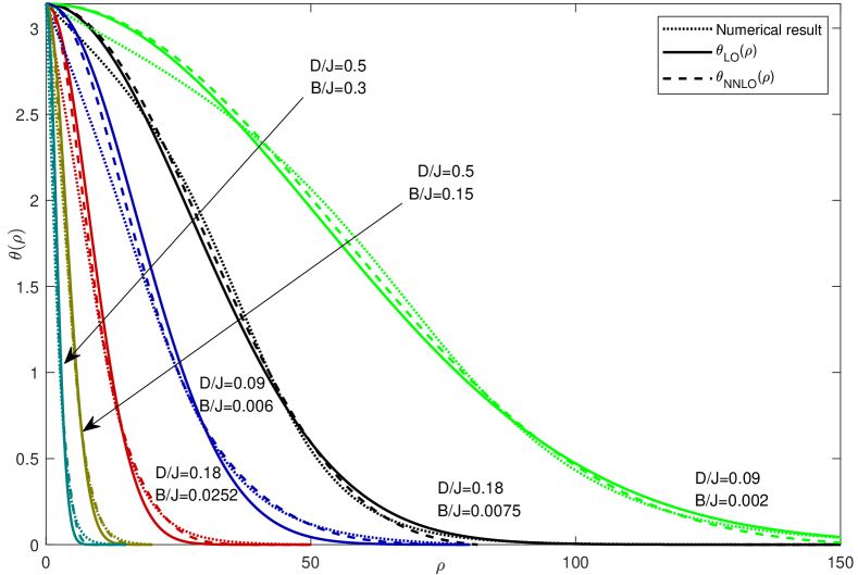
Figure 2: The numerical result together with the results from $\theta_{\rm LO}(\rho)$ and $\theta_{\rm NNLO}(\rho)$. The dotted lines represent numerical results, the solid lines represent $\theta_{\rm LO}$, the dashed lines represent $\theta_{\rm NNLO}$. The parameters $J$, $D$ and $B$ are chosen to be such that the system is in the skyrmion phase, that is, $D/J=0.18$ while $0.0075<B/J<0.0252$ ThieleStudyAndJDB , $D/J=0.09$ while $0.001875<B/J<0.0063$JDBRef1 , and $D/J=0.5$ while $0.15<B/J<0.30$ JDBRef2 .

III Lattice Simulation

To verify the the variational calculation, we also study the radii of the skyrmions by doing the lattice simulation, which is based on the LLG equation nagaosa ; pin ; LLG ; LLG2

$$\begin{split}&\frac{d}{dt}{\bf n}_{\bf r}=-{\bf B}_{\rm eff}({\bf r})\times{\bf n}_{\bf r}-\alpha{\bf n}_{\bf r}\times\frac{d}{dt}{\bf n}_{\bf r},\\ \end{split}$$ (17)

where ${\bf n}_{\bf r}$ is the local magnetic momentum at site ${\bf r}$, $\alpha$ is the Gilbert damping constant,

$$\begin{split}&{\bf B}_{\rm eff}({\bf r})=-\frac{\delta H}{\delta{\bf n}_{\bf r}}\end{split}$$ (18)

is the effective magnetic field, with the discrete Hamiltonian $H$ JDBRef1 ; ThieleStudyAndJDB

$$\begin{split}&H=\sum_{{\bf r},i=x,y}\left[-J({\bf r}){\bf n}_{{\bf r}+\delta_{i}}-D({\bf r}){\bf n}_{{\bf r}+\delta_{i}}\times{{\bf e}}_{i}-{\bf B}\right]\cdot{\bf n}_{\bf r},\\ \end{split}$$ (19)

where $\delta_{i}$ refers to each neighbour, and $\delta_{i}={\bf e}_{i}$ on a square lattice. So pin

$$\begin{split}&{\bf B}_{\rm eff}({\bf r})=\sum_{i=x,y}\left[J({\bf r}){\bf n}_{{\bf r}+\delta_{i}}+J({\bf r}-\delta_{i}){\bf n}_{{\bf r}-\delta_{i}}\right]\\ &+\sum_{i=x,y}\left[D({\bf r}){\bf n}_{{\bf r}+\delta_{i}}\times{{\bf e}}_{i}-D({\bf r}-\delta_{i}){\bf n}_{{\bf r}-\delta_{i}}\times{{\bf e}}_{i}\right]+{\bf B}({\bf r}).\end{split}$$ (20)

We run the simulation on a $512\times 512$ square lattice. The simulation was done by using the GPU program . The LLG is numerically integrated by using the fourth-order Runge-Kutta method. We run the simulation with $D/J=0.18$ and with $B/J=0.012,0.015,0.018,0.024$ such that $0.009<B/J<0.0252$, and it is set that $\alpha=0.04$ ThieleStudyAndJDB and time step $\Delta t=0.01$. To study the radii of skyrmions with different $J$, we run the simulation with $J=1,2,3,4,5$.

We study both an isolated skyrmion and the skyrmion phase. For the isolated skyrmion, we run the simulation with periodic boundary condition and with the initial state ${\bf n}_{r}={\bf e}_{z}$, except ${\bf n}_{r}=-{\bf e}_{z}$ when the sites are near the center, with $|{\bf r}-(255,255)|<10$. Under such initial condition, a single skyrmion can be created at the center, due to the mechanism similar to that in Ref. Romming , where a skyrmion can be created at a desired position by flipping the spin at the position. To study the skyrmion phase, we run the simulation with open boundary condition and with randomized initial configurations.

To evaluate the radius $r_{s}$ of the skyrmion, one needs to calculate the number of the sites in the isoheight contour of $n_{z}=1$. However, $n_{z}$ only approaches $1$, so we use the isoheight contour of $n_{z}=0.5$ and compare $r_{s}$ with the solutions $\rho$ of the equations $\theta_{\rm LO}(\rho)=\cos^{-1}(0.5)$ and $\theta_{\rm NNLO}(\rho)=\cos^{-1}(0.5)$. The details on how the radii are obtained can be found in Appendix, and the results are shown in Fig. 3. One can find that the value of $J$ has little effect when dimensionless parameters are used, as discussed in Sec. II. In the case of an isolated skyrmion, the radii obtained from $\theta_{\rm LO}(\rho)$ fit the simulation results well, and those calculated obtained from $\theta_{\rm NNLO}(\rho)$ fit the simulation results even better. For the skyrmions in the skyrmion phase, their radii are smaller than those of isolated skyrmions. This is because the skyrmions are now crowded, and are constrained by the domain walls of the neighbouring skyrmions, consequently the skyrmions shrink.

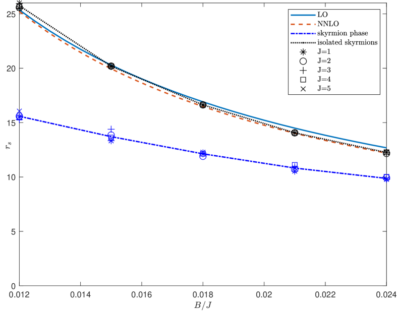
Figure 3: The radii $r_{s}$’s of the skyrmions, obtained from the simulation and from $\theta_{\rm LO}(\rho)$ and $\theta_{\rm NNLO}(\rho)$. The solid line represents the solution of $\theta_{\rm LO}(\rho)=\cos^{-1}(0.5)$, and the dashed line represents the solution of $\theta_{\rm NNLO}(\rho)=\cos^{-1}(0.5)$. The dotted line and the dashed dotted line are guides to the eyes. For an isolated skyrmion, $\theta_{\rm LO}(\rho)$ fits the simulation result well and $\theta_{\rm NNLO}(\rho)$ fits it even better. For the skyrmions in the skyrmion phase, the radii of the skyrmions are smaller than those of the isolated skyrmions, because the skyrmions are then crowded and constrained by the neighbouring skyrmions.

Using dimensionless parameters, $J$ is an energy unit JDBRef1 ; alpha3 ; bilayer2 , and is also related to the rescaling of the lattice. To make correspondence with the real material, we use the rescaling method in Refs. Tchoe ; pin . The lattice rescaling factor $r$ is related to helical wavelength $\lambda$ and the lattice spacing $a$ as $r=(D/J)\lambda/\left(2\pi\sqrt{2}a\right)$, and the time unit is rescaled as $t^{\prime}=r^{2}t$. For example, if for a real material, we have $\lambda\approx 60\;{\rm nm}$, $a\approx 4\;{\AA}$ and $D/J=0.18$, we find $r\approx 3.04$, therefore $\rho=1$ corresponds to $\rho\approx 1.22{\rm nm}$. Hence $r_{s}=15.5176$ corresponds to $18.87{\rm nm}$. The unit of time rescales with the dimensionless $J$ and exchange strength of real material $J^{\prime}$ as $t^{\prime}=r^{2}J\hbar/J^{\prime}$. For the case of $J=1$, if we adopt $J^{\prime}=3\;{\rm meV}$, then $t^{\prime}=r^{2}J\hbar/J^{\prime}\approx 220r^{2}\;{\rm fs}\approx 0.02\;{\rm ns}$, thus the time step in the simulation corresponds to $\Delta t\approx 20.3{\rm fs}$.

IV Applications

One can predict the skyrmion’s behaviour associated with $\theta(\rho)$ by using $\theta_{\rm LO}(\rho)$ or $\theta_{\rm NNLO}(\rho)$. Besides, when the relation between the behaviour of the skyrmions and the parameters $J$, $B$ and $D$ can be expressed explicitly, one is able to use such expressions as a guidance to choose the parameter values of $J$, $B$ and $D$ in experiments. In the following, we give two examples showing that the problems can be greatly simplified by using our method.

IV.1 Thiele Equation

The motion of a skyrmion can be described in terms of the Thiele equation

$$0=-f_{\rm pin}^{\mu}+g\epsilon^{\mu\nu}\left(v_{\nu}-j_{\nu}\right)+d^{\mu\nu}\left(\alpha v_{\nu}-j_{\nu}\right),$$ (21)

where $f_{\rm pin}^{\mu}$ is the pinning force, $g=4\pi Q$ is the gyromagnetic coupling proportional to the skyrmion number $Q$, $\epsilon^{\mu\nu}$ is the Kronecker tensor, $v$ is the collective velocity of skyrmion and $j$ is the external electrical current, $\alpha$ is the Gilbert damping coefficient, $d^{\mu\nu}$ is the dissipative matrix given by

$$d^{\mu\nu}=\int d^{2}r\left(\partial_{\mu}\vec{n}\right)\cdot\left(\partial_{\nu}\vec{n}\right).$$ (22)

From Eq. (1), we find

$$\begin{split}&d^{xy}=d^{yx}=0,\;\;d^{xx}=d^{yy}=2\pi d_{0},\end{split}$$ (23)

with

$$\begin{split}&d_{0}\equiv\int_{0}^{\infty}d\rho\frac{\sin^{2}\left(\theta(\rho)\right)+\rho^{2}\left(\frac{\partial\theta(\rho)}{\partial\rho}\right)^{2}}{2\rho},\end{split}$$ (24)

which, according to $\theta_{\rm NNLO}(\rho)$ given in Eq. (14), can be written as

$$\begin{split}&d_{0}\approx c_{1}+c_{2}b+\mathcal{O}(b^{2}),\\ \end{split}$$ (25)

where $b$ are parameters in Eq. (16), and

$$\begin{split}&c_{1}=\int_{0}^{\infty}dy\left(\frac{\pi^{2}e^{-y}y^{2}+\sin^{2}\left(\pi e^{-\frac{y}{2}}\right)}{4y}\right)\approx 2.8991,\\ &c_{2}=\frac{1}{2}\left(-\text{Ci}(2\pi)-2\pi^{2}+\gamma_{E}+\log(2\pi)\right).\\ \end{split}$$ (26)

Note that $c_{1}$ is the LO contribution while the $c_{2}b$ is the NNLO contribution. Using the results of $c_{1}$, $c_{2}$ and $b$, we find

$$\begin{split}&d_{0}\approx 3.75553+\frac{\frac{B}{J}\left(0.582005\left(\frac{D}{J}\right)^{2}-1.75302\frac{B}{J}\right)}{\left(\frac{B}{J}\right)^{2}+0.013875\frac{B}{J}\left(\frac{D}{J}\right)^{2}-0.114832\left(\frac{D}{J}\right)^{4}}.\end{split}$$ (27)

Now we compare this result with the numerical result, as shown in Figs. 4 and 5, for the parameter regimes studied in Refs. ThieleStudyAndJDB ; JDBRef1 ; JDBRef2 . We find that our variational calculation agrees with the numerical result well. The discrepancy increases with the deviation of $d_{0}$ from $c_{1}$, because as $\theta(\rho)$ deviates from $\phi_{0}$, the higher order terms become important.

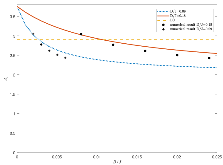
Figure 4: Comparison of the results on the dissipative matrix element $d_{0}$ from our analytical expression $\theta_{\rm NNLO}$ and from numerical calculation. The dotted line represents the analytical result from $\theta_{\rm NNLO}$ for $D/J=0.09$, the solid line represents the analytical result from $\theta_{\rm NNLO}$ for $D/J=0.18$. The plus signs represent numerical results for $D/J=0.09$ and $B/J=0.002,0.003,0.004,0.005,0.006$. The filled circles represent numerical results for $D/J=0.18$ and $B/J=0.008,0.012,0.016,0.020,0.024$. The dashed line represents the analytical result from $\theta_{\rm LO}$.

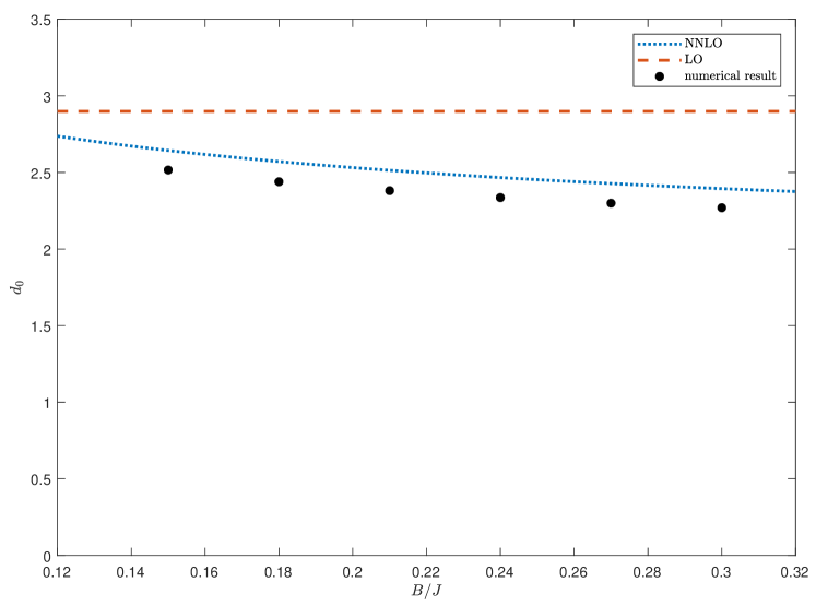
Figure 5: Comparison of the results on the dissipative matrix element $d_{0}$ from our analytical expression $\theta_{\rm NNLO}$ and from numerical calculation. The dotted line represents the analytical result from $\theta_{\rm NNLO}$ for $D/J=0.5$. The filled circles represent numerical results for $D/J=0.5$ and $B/J=0.15,0.18,0.21,0.24,0.27,0.3$. The dashed line represents the analytical result from $\theta_{\rm LO}$.

IV.2 Interaction of skyrmions in a bilayer system

The interaction between two skyrmions on two separated and overlapped planes is an interesting problem studied in Ref. bilayer2 using micromagnetic simulations as well as the analysis based on Thiele equation. When two skyrmions are close to each other, $\theta(\rho)$ plays an important role in the interaction between the two skyrmions.

The normalized potential between two skyrmions can be written as bilayer2

$$\begin{split}&u({\bf r}_{d})=\int d^{2}r\left(1-{\rm sign}(J_{\rm inter}){\bf n}_{1}({\bf r}-\frac{{\bf r}_{d}}{2})\cdot{\bf n}_{2}({\bf r}+\frac{{\bf r}_{d}}{2})\right),\\ \end{split}$$ (28)

where ${\bf n}_{1}$ and ${\bf n}_{2}$ are magnetic moments of the two skyrmions, $J_{\rm inter}$ is the Heisenberg coupling between two layers, ${\bf r}_{d}$ is the distance between the two skyrmions. Suppose the DM interaction strengths of the two skrymions are $D_{1}$ and $D_{2}$, respectively.

To study the case of $D_{1}=-D_{2}$, one needs to consider a more general parameterization nagaosa

$$\begin{split}&{\bf n}({\bf r})=\left(\cos(\gamma+m\phi)\sin(\theta(\rho)),\sin(\gamma+m\phi)\sin(\theta(\rho)),g\cos(\theta(\rho))\right),\\ \end{split}$$ (29)

where $(\phi,\rho)$ is ${\bf r}$ in polar coordinates, $\gamma$ is the helicity angle, $m=1$ for a skyrmion and $m=-1$ for an anti-skyrmion, $g=\pm 1$. The skyrmion number is

$$\begin{split}&Q=\frac{1}{4\pi}\int dxdy{\bf n}\cdot\left(\frac{\partial{\bf n}}{\partial x}\times\frac{\partial{\bf n}}{\partial y}\right)=-mg.\\ \end{split}$$ (30)

With isotropic DM interaction, we consider the case of $m=1$ antiskyrmion . The Euler-Lagrange equation yields

$$\begin{split}&\frac{\sin(\theta)\cos(\theta)}{\rho}-\theta^{\prime}-\rho\theta^{\prime\prime}-2\frac{\hat{D}}{J}\sin^{2}(\theta)+\frac{\hat{B}}{J}\rho\sin(\theta)=0,\end{split}$$ (31)

with $\hat{D}\equiv g\sin(\gamma)D$, $\hat{B}\equiv gB$. The parameters in Eq. (1) correspond to $g=1$ and $\gamma=\pi/2$ here. $D<0$ case in Ref. bilayer2 correspond to $g=1$ and $\gamma=3\pi/2$. For $D_{2}=-D_{1}$, by setting $\gamma=3\pi/2$, the equation of motion of $\theta(\rho)$ is the same as that for $D_{1}$ with $\gamma=\pi/2$. As a result, in considering the two interacting skrymions, with $D_{1}=D_{2}$ or $D_{1}=-D_{2}$, we have two skyrmions with the same size and same shape $\theta(\rho)$. Suppose the intralayer Hamiltonians dominate the interlayer interaction, the effect of inter-skyrmion interaction on $\theta(\rho)$ can be neglected. Consequently, one can use the functions $\theta_{\rm LO}$ and $\theta_{\rm NNLO}$ above for each skyrmion.

For $D_{1}=\pm D_{2}$, we define the corresponding normalized potential as $u_{\pm}({\bf r}_{d})$,

$$\begin{split}&u_{\pm}({\bf r}_{d})=\int d^{2}r\left[1-\cos\left(\theta(|{\bf r}+\frac{{\bf r}_{d}}{2}|)\right)\cos\left(\theta(|{\bf r}-\frac{{\bf r}_{d}}{2}|)\right)\right.\\ &\left.\mp\frac{\left(r^{2}-\frac{{\bf r}_{d}^{2}}{4}\right)\sin\left(\theta(|{\bf r}+\frac{{\bf r}_{d}}{2}|)\right)\sin\left(\theta(|{\bf r}-\frac{{\bf r}_{d}}{2}|)\right)}{|{\bf r}+\frac{{\bf r}_{d}}{2}||{\bf r}-\frac{{\bf r}_{d}}{2}|}\right].\\ \end{split}$$ (32)

Note that both $\theta_{\rm LO}(\rho)$ and $\theta_{\rm NNLO}(\rho)$ are functions of $-\omega\rho^{2}$ and can be written as $\theta^{\prime}(-\omega\rho^{2}/2)$, for simplicity, we can take the ${\bf x}$-axis as the direction of ${\bf r}_{d}$ and rewrite $u_{\pm}$ as

$$\begin{split}&u_{\pm}(r_{d})=\frac{1}{\omega}\bar{u}_{\pm}(\frac{\sqrt{\omega}r_{d}}{2}),\\ \end{split}$$ (33)

where

$$\begin{split}&\bar{u}_{\pm}(r^{\prime}_{d})=\int dxdy\left[1-\cos\left(\theta^{\prime}(-\frac{1}{2}((x+r^{\prime}_{d})^{2}+y^{2}))\right)\cos\left(-\frac{1}{2}((x-r^{\prime}_{d})^{2}+y^{2}))\right)\right.\\ &\left.\mp\frac{\left(x^{2}+y^{2}-(r^{\prime}_{d})^{2}\right)\sin\left(\theta^{\prime}(-\frac{1}{2}((x+r^{\prime}_{d})^{2}+y^{2}))\right)\sin\left(\theta^{\prime}(-\frac{1}{2}((x-r^{\prime}_{d})^{2}+y^{2}))\right)}{\sqrt{(x+r^{\prime}_{d})^{2}+y^{2}}\sqrt{(x-r^{\prime}_{d})^{2}+y^{2}}}\right],\\ \end{split}$$ (34)

with $2r^{\prime}_{d}$ being the rescaled dimensionless distance of the two skyrmions. $\bar{u}_{\pm}(r^{\prime}_{d})$ is a function independent of $J$, $B$ and $D$, and can be used for various values of $J$, $B$ and $D$.

It is difficult to obtain the analytical result of $\bar{u}_{\pm}(r_{d})$, so we use Pad${\rm\acute{e}}$ approximants pade ; padeapp . When the two skyrmions are far away from each other, the skyrmions should be independent of each other, so the functions $\bar{u}_{\pm}(r_{d}^{\prime})$ should asymptotically become constants. Numerically we find $|\partial_{r_{d}}\bar{u}_{\pm}(3)|<0.02$, so we use k-points $[m,n]$ order Pad${\rm\acute{e}}$ approximation to write $\bar{u}_{\pm}(r_{d}^{\prime})$ as

$$\begin{split}&\bar{u}_{\pm}(r^{\prime}_{d})\approx\left\{\begin{array}[]{c}\tilde{u}_{\pm}(r^{\prime}_{d}),\;\;0\leq r^{\prime}_{d}\leq 3;\\ \tilde{u}_{\pm}(3),\;\;r^{\prime}_{d}>3,\end{array}\right.\end{split}$$ (35)

where

$$\begin{split}&\tilde{u}_{\pm}(r^{\prime}_{d})=\frac{\sum_{i=0}^{m}p_{i}{r^{\prime}_{d}}^{i}}{1+\sum_{j=1}^{n}q_{j}{r^{\prime}_{d}}^{j}}.\end{split}$$ (36)

We use three-point $[5,4]$ order Pad${\rm\acute{e}}$ approximants where $p_{0,\ldots,4}$ and $q_{1,\ldots,4}$ are $9$ constants independent of $J$, $D$ and $B$ and can be determined from equations

$$\begin{split}&\tilde{u}_{\pm}(r^{\prime}_{d})-\bar{u}_{\pm}(r^{\prime}_{d})=0+\mathcal{O}\left((r^{\prime}_{d}-r^{\prime}_{k})^{l}\right),\\ \end{split}$$ (37)

where $k=1,2,3$,$r^{\prime}_{1,2,3}=0,3/2,3$, $l=3$. Using $\theta_{\rm LO}(\rho)$, we find

$$\begin{split}&u_{\pm}(r_{d})\approx\left\{\begin{array}[]{c}u_{\rm\pm LO}(r_{d}),\;\;0\leq r_{d}\leq r_{d\;max};\\ u_{\rm\pm LO}(r_{d\;max}),\;\;r_{d}>r_{d\;max}.\end{array}\right.\\ \end{split}$$ (38)

with $r_{d\;max}=6/\sqrt{\omega_{\rm LO}}$,

$$\begin{split}&u_{\rm+LO}(r_{d})=\frac{D^{2}r_{d}^{2}\left(0.625637B^{2}r_{d}^{2}-4.20541BDr_{d}+9.10783D^{2}\right)}{0.0240738B^{4}r_{d}^{4}-0.177479B^{3}Dr_{d}^{3}+0.532727B^{2}D^{2}r_{d}^{2}-0.751001BD^{3}r_{d}+D^{4}},\\ &u_{\rm-LO}(r_{d})=\frac{D^{2}\left(25.9614B^{4}r_{d}^{4}-281.728B^{3}Dr_{d}^{3}+1249.66B^{2}D^{2}r_{d}^{2}-3067.97BD^{3}r_{d}+5066.63D^{4}\right)}{B^{2}\left(B^{4}r_{d}^{4}-11.4014B^{3}Dr_{d}^{3}+55.5842B^{2}D^{2}r_{d}^{2}-153.947BD^{3}r_{d}+254.237D^{4}\right)}.\\ \end{split}$$ (39)

We also calculate $u_{\pm}(r_{d})$ using the numerical result of $\theta(\rho)$ for $D/J=0.18$ and $B/J=0.0164$, in the regime of the skyrmion phase studied in Ref. ThieleStudyAndJDB . The numerical result and the leading order approximation are shown in Fig. 6. Up to LO, our analytical result fits the numerical result well. It is also very convenient to obtain the interaction between the two skyrmions using $F(r_{d})=-|J_{\rm inter}|\partial_{r_{d}}u(r_{d})$ bilayer2 and Eq. (39). The function $-\partial_{r_{d}}u_{\rm\pm LO}(r_{d})$ is also shown in Fig. 6.

\begin{overpic}[width=346.89731pt]{urd} \put(40.0,10.0){\includegraphics[width=186.45341pt]{force}} \end{overpic}

Figure 6: The normalized potentials obtained from $\theta_{\rm LO}$ and from numerical calculation. The solid line represents $u_{\rm+LO}(r_{d})$, while the stars represent $u_{+}(r_{d})$ from numerical calculation. The dashed line represents $u_{\rm-LO}(r_{d})$, while the plus dots represent $u_{-}(r_{d})$ from numerical calculation. The results are given for $D/J=0.18$ and $B/J=0.0164$. When $r_{d}>r_{d\;max}\approx 75.12$, $u_{\pm}(r_{d})\approx u_{\rm LO}(r_{d\;max})$ is about a constant. The interaction $-\partial_{r_{d}}u$ between two skyrmions are also determined. $-\partial_{r_{d}}u<0$ means attractive force between the skyrmions, while $-\partial_{r_{d}}u>0$ means repulsive force between the skyrmions.

V Summary

As a topological soliton, a skyrmion is often treated as a point-like particle on large scales. However, when the scale of the dynamics is comparable with the radius of the skyrmion, we need to consider the shape of the skyrmion. Moreover, we need $\theta(\rho)$ to determine the dissipative matrix in the Thiele equation. Hence the study of the $\theta(\rho)$ is both interesting and important.

In this paper, we propose a method to represent $\theta(\rho)$ approximately yet efficiently in terms of the eigenfunctions of Schrödinger operator of the harmonic oscillator. Using variational approach, we find that the result can be written as a superposition of the first few eigenfunctions Eqs. (14), and we have determined that superposition coefficients as well as the frequency of the harmonic oscillator as a function of the parameters of the magnetic system. Using the result, we are immediately able to calculate the radii of the skrymions, which are verified by the numerical calculation and also by lattice simulation. We also use our method to study the dissipative matrix in the Thiele equation. We obtain the matrix elements as explicit functions of the parameters $B$, $J$ and $D$, which agree with the numerical results. We also use our method to study the interaction between two skyrmions on two layers, with result confirmed by the numerical calculation.

This work is supported by National Natural Science Foundation of China (Grant No. 11374060 and No. 11574054).

Appendix A Supplemental information

A.1 Ansatz functions as examples of harmonic oscillator expansion

One can choose any complete set of orthogonal functions to expand $\theta(\rho)$. For better convergence, we choose the eigenfunctions of harmonic oscillator such that the LO wave function is close to the numerical results. As examples, we obtain the harmonic oscillator expansions of the ansatz functions of $\theta(\rho)$ used in previous works, in which $\theta(\rho)$ is linear in $\rho$ Jiang ; NParameterAndLinear ; thetarho , or satisfy $\theta(\rho)=\arctan\left(\exp\left(-\rho/\Delta\right)\right)$ NParameterArcTan ; arctan .

The results are listed in Table. A1 and shown in Fig. A1, with $\omega$ arbitrarily set to be $1$. Among these examples, the functions $f_{1}(x)$ and $f_{2}(x)$ are the ansatz functions for $\theta(\rho)$ in Ref. Jiang ; NParameterAndLinear ; NParameterArcTan ; thetarho , while the functions $f_{3}(x)$ and $f_{4}(x)$ are the ansatz functions for $\theta(\rho)$ in Ref. arctan ; NParameterArcTan . It can be seen that the expansions approximate the original functions very well.

Table A1: The harmonic oscillator expansion of some functions, which were previously used for $\theta(\rho)$, and are also shown in Fig. A1. $\omega$ is arbitrarily set to be 1.

$f(x)\approx\sum_{\begin{subarray}{c}n=0\end{subarray}}^{5}C_{n}\phi_{2n,\omega}(x)$	$C_{0}$	$C_{1}$	$C_{2}$	$C_{3}$	$C_{4}$	$C_{5}$
$f_{1}(x)=\left\{\begin{array}[]{c}\pi-x,\;\;x\in[0,\pi];\\ 0,\;\;x>\pi.\end{array}\right.$	4.414	1.012	0.354	-0.173	-0.042	0.009
$f_{2}(x)=\left\{\begin{array}[]{c}\pi,\;\;x\in[0,\frac{\pi}{2});\\ \frac{3\pi}{2}-x,\;x\in[\frac{\pi}{2},\frac{3\pi}{2}],\\ 0,\;x>\frac{3\pi}{2}.\end{array}\right.$	5.821	3.498	1.969	1.101	0.650	0.168
$f_{3}(x)=4\tan^{-1}(\exp(-x))$	3.486	0.069	0.428	-0.031	0.157	-0.040
$f_{4}(x)=\left\{\begin{array}[]{c}\pi,\;\;x\in[0,\frac{\pi}{2}];\\ 4\tan^{-1}\left(e^{-(x-\frac{\pi}{2})}\right),\;\;x>\frac{\pi}{2}.\end{array}\right.$	5.746	3.000	1.014	0.371	0.407	0.117

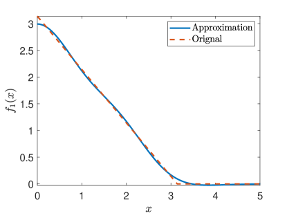
(a) $f_{1}(x)$

(b) $f_{2}(x)$

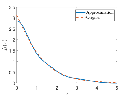
(c) $f_{3}(x)$

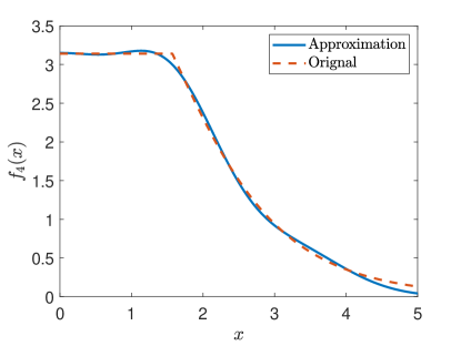
(d) $f_{4}(x)$

Figure A1: The harmonic oscillator expansion of some functions listed in Table. A1. $\omega$ is arbitrarily set to be $1$. In each plot, the dashed line is for the function while the solid line is for the expansion $\sum_{n=0}^{5}C_{n}\phi_{2n,\omega}(x)$. These functions have been used for $\theta(\rho)$ previously.

In the above examples, an arbitrary value of $\omega$ was used. However, an appropriate value of $\omega$ leads to better convergence.

A.2 The solution at NNLO

Substitute the trial solution Eq. (14) for $F$ in Eqs. (3) and (4). By minimizing $F$, one obtains three equations with three undetermined variables.

The equation $dF/db=0$ leads to Eq. (15) with

$$\begin{split}&a_{111}=-\text{Ci}(2\pi)-2\pi^{2}+\gamma_{E}+\log(2\pi)\approx-17.3016,\\ &a_{112}=2\pi^{2}\left(\;{}_{3}F_{4}\left(\left.\begin{array}[]{c}1,1,1\\ \frac{1}{2},2,2,2\end{array}\right|-\pi^{2}\right)+2\right)\approx 39.1263,\\ &a_{113}=6\pi^{2}\left(\;{}_{4}F_{5}\left(\left.\begin{array}[]{c}1,1,1,1\\ \frac{1}{2},2,2,2,2\end{array}\right|-\pi^{2}\right)+4\right)\approx 255.4126,\\ &a_{211}=0,\;\;\;a_{212}=-a_{111},\;\;\;a_{213}=a_{112},\;\;a_{311}=a_{312}=a_{313}=0,\\ \end{split}$$ (A1)

while $dF/da=0$ leads to

$$\begin{split}&a_{121}=\int_{0}^{\infty}dy\left(\pi e^{-\frac{y}{2}}y^{3/2}\left(-y+\cos\left(2\pi e^{-\frac{y}{2}}\right)+4\right)\right)\approx-13.4774,\\ &a_{122}=\int_{0}^{\infty}dy\left(-2\left(\pi^{2}e^{-y}y^{5/2}\sin\left(2\pi e^{-\frac{y}{2}}\right)\right)\right)\approx-36.5000,\\ &a_{123}=\int_{0}^{\infty}dy\left(-2\left(\pi^{2}e^{-y}y^{7/2}\sin\left(2\pi e^{-\frac{y}{2}}\right)\right)\right)\approx-129.3094,\\ &a_{221}=\int_{0}^{\infty}dy\left(\pi e^{-\frac{y}{2}}\sqrt{y}\left(-y+\cos\left(2\pi e^{-\frac{y}{2}}\right)+2\right)\right)\approx-7.5206,\\ &a_{222}=\int_{0}^{\infty}dy\left(-2\left(\pi^{2}e^{-y}y^{3/2}\sin\left(2\pi e^{-\frac{y}{2}}\right)\right)\right)\approx-9.0845,\\ &a_{223}=a_{122},\;\;\;a_{321}=a_{322}=-\frac{1}{2}a_{221},\;\;\;a_{323}=-\frac{1}{2}a_{121},\\ \end{split}$$ (A2)

and $dF/d\omega=0$ leads to

$$\begin{split}&a_{131}=-2\pi^{2}\;_{3}F_{4}\left(\left.\begin{array}[]{c}1,1,1\\ \frac{3}{2},2,2,2\end{array}\right|-\frac{\pi^{2}}{4}\right)\approx-16.2190,\\ &a_{132}=-6\pi^{2}\;_{4}F_{5}\left(\left.\begin{array}[]{c}1,1,1,1\\ \frac{1}{2},2,2,2,2\end{array}\right|-\frac{\pi^{2}}{4}\right)\approx-43.6330,\\ &a_{133}=-24\pi^{2}\;_{5}F_{6}\left(\left.\begin{array}[]{c}1,1,1,1,1\\ \frac{1}{2},2,2,2,2,2\end{array}\right|-\frac{\pi^{2}}{4}\right)\approx-204.0066,\\ &a_{231}=-4(-\text{Ci}(\pi)+\gamma_{E}+\log(\pi))\approx-6.5931,\\ &a_{232}=-2\pi^{2}\;_{3}F_{4}\left(\left.\begin{array}[]{c}1,1,1\\ \frac{1}{2},2,2,2\end{array}\right|-\frac{\pi^{2}}{4}\right)\approx-10.1534,\\ &a_{233}=a_{132},\;\;a_{331}=-\frac{1}{2}a_{231},\;\;a_{332}=-a_{231},\;\;a_{333}=-a_{131},\\ \end{split}$$ (A3)

where ${}_{p}F_{q}$ are hypergeometric functions.

The solution can be written as

$$\begin{split}&a\approx\frac{k_{3}k_{4}-k_{1}k_{6}}{k_{2}k_{6}-k_{3}k_{5}},\;\;\;\;b\approx\frac{k_{2}k_{4}-k_{1}k_{5}}{k_{3}k_{5}-k_{2}k_{6}},\\ &\sqrt{\omega}\approx\frac{B(a_{331}+a_{332}a+a_{333}b)}{D(a_{321}+a_{322}a+a_{323}b)},\\ \end{split}$$ (A4)

with

$$\begin{split}&k_{1}=\frac{1}{2}\left(\frac{\left(\frac{D}{J}\right)^{2}a_{321}(a_{121}a_{331}-a_{131}a_{321})}{\frac{B}{J}a_{331}^{2}}+a_{111}\right),\\ &k_{2}=\frac{1}{2}\left\{\frac{\left(\frac{D}{J}\right)^{2}}{\frac{B}{J}a_{331}^{3}}\left[a_{331}\left(a_{121}a_{322}a_{331}+a_{122}a_{321}a_{331}-2a_{131}a_{321}a_{322}-a_{132}a_{321}^{2}\right)\right.\right.\\ &\left.\left.+a_{321}a_{332}(2a_{131}a_{321}-a_{121}a_{331})\right]+a_{112}\right\},\\ &k_{3}=\frac{1}{2}\left\{\frac{\left(\frac{D}{J}\right)^{2}}{\frac{B}{J}a_{331}^{3}}\left[a_{331}\left(a_{121}a_{323}a_{331}+a_{123}a_{321}a_{331}-2a_{131}a_{321}a_{323}-a_{133}a_{321}^{2}\right)\right.\right.\\ &\left.\left.+a_{321}a_{333}(2a_{131}a_{321}-a_{121}a_{331})\right]+a_{113}\right\},\\ &k_{4}=\frac{\left(\frac{D}{J}\right)^{2}a_{321}(a_{221}a_{331}-a_{231}a_{321})}{2\frac{B}{J}a_{331}^{2}},\\ &k_{5}=\frac{1}{2}\left\{\frac{\left(\frac{D}{J}\right)^{2}}{\frac{B}{J}a_{331}^{3}}\left[a_{331}\left(a_{221}a_{322}a_{331}+a_{222}a_{321}a_{331}-2a_{231}a_{321}a_{322}-a_{232}a_{321}^{2}\right)\right.\right.\\ &\left.\left.+a_{321}a_{332}(2a_{231}a_{321}-a_{221}a_{331})\right]+a_{212}\right\},\\ &k_{6}=\frac{1}{2}\left\{\frac{\left(\frac{D}{J}\right)^{2}}{\frac{B}{J}a_{331}^{3}}\left[a_{331}\left(a_{221}a_{323}a_{331}+a_{223}a_{321}a_{331}-2a_{231}a_{321}a_{323}-a_{233}a_{321}^{2}\right)\right.\right.\\ &\left.\left.+a_{321}a_{333}(2a_{231}a_{321}-a_{221}a_{331})\right]+a_{213}\right\}.\\ \end{split}$$ (A5)

A.3 Radii of the skyrmions in simulations

In the lattice simultion, we use the initial condition and the parameters in Sec. III, and we obtain isolated skyrmions as well as skyrmion phases. Some examples are shown in Figs. A2 and A3.

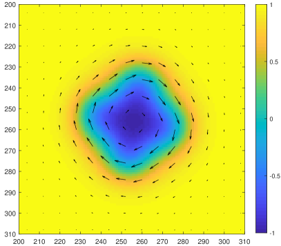
(a) $J=3,B/J=0.012$

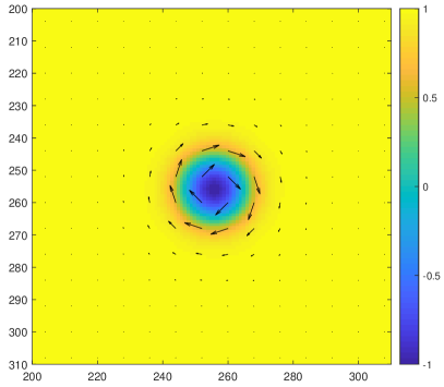
(b) $J=3,B/J=0.024$

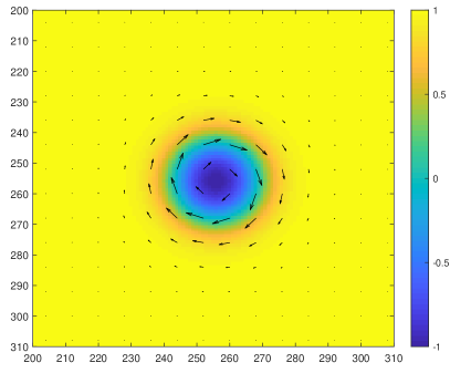
(c) $J=1,B/J=0.018$

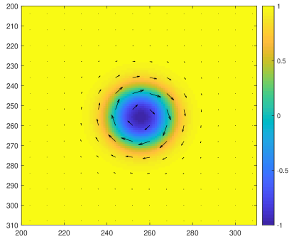
(d) $J=5,B/J=0.018$

Figure A2: Simulation result with an isolated skyrmion. The heat map represents the magnitude of $n_{z}$ and each arrow represents $(n_{x},n_{y})$. One can find from the value of $J$ has little effect when using dimensionless parameters.

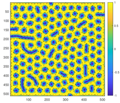
(a) $J=3,B/J=0.012$

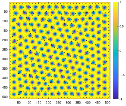
(b) $J=3,B/J=0.024$

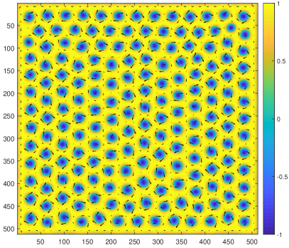
(c) $J=1,B/J=0.018$

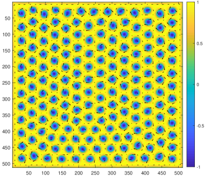
(d) $J=5,B/J=0.018$

Figure A3: Simulation result with a skyrmion phase. One can notice that the value of $J$ has little effect when using dimensionless parameters.

To approximately calculate the skyrmion radius $r_{s}$, we use the isoheight contour of $n_{z}=0.5$, i.e. we count the number $N$ of sites with $n_{z}<0.5$, and the radius is estimated as $r_{s}=\sqrt{N/\pi}$. For an isolated skyrmion, this procedure is straightforward. For a skyrmion phase, we first calculate the isoheight contours of $n_{z}=0.5$, then we discard the contours adjacent to the edge. After that, we remove those contours with radii larger than $150\%$ of the median radius. As an example, we establish the case for $J=1,B/J=0.12$ in Fig. A4. In Fig. A4.(c), we obtain $115$ skyrmions with average radius $r_{s}\approx 15.5176$.

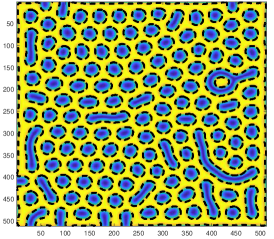
(a) We first calculate the isoheight contours with $n_{z}=0.5$ (dashed lines).

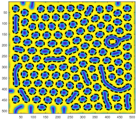
(b) Then we remove contours adjacent to the edge.

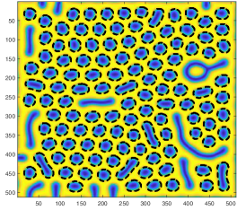
(c) Then we remove the contours with radius larger than $150\%$ of the median radius of the contours.

Figure A4: Illustration on how we calculate the radii of the skyrmions. $J=1,B/J=0.012$. There are $115$ skyrmions with average radius $r_{s}\approx 15.5176$.

In Sec. II and Sec. III, we find that both the numerical results and simulation results can by well fitted by our analytical calculation results. In fact, the numerical results are very closed to the results of isolated skyrmions in the simulation, it is therefore sufficient to verify only the numerical results in the case of isolated skyrmions. We show an example for $J=1$ and $B/J=0.018$ (same as Fig. A2.(c)) in Fig. A5.

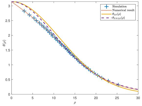
Figure A5: Comparison of the simulation result for an isolated skyrmion, the numerical result, $\theta_{\rm LO}$ and $\theta_{\rm NNLO}$ with $J=1$, $D=0.18$ and $B=0.018$. The plus signs represent the average radii of the isoheight contours of $n_{z}$ in simulation. The dotted line represents the numerical result, the solid line represents $\theta_{\rm LO}$, and the dashed line represents $\theta_{\rm NNLO}$. The numerical result is very close to the simulation result.

References

- (1) N. Nagaosa and Y. Tokura, Nat. Nanotechnol. 8, 899 - 911 (2013).
- (2) A. Fert, N. Reyren and V. Cros, Nat. Rev. Mater. 2, 17031 (2017).
- (3) S. Mühlbauer et. al. Science 323, 915 - 919 (2009).
- (4) X. Z. Yu et. al. Nature 465, 901 - 904 (2010).
- (5) S. Heinze et. al. Nat. Phys. 7, 713 - 718 (2011); C. Pfleiderer, Nature Phys. 7, 673 - 674 (2011).
- (6) F. Jonietz et. al. Science 330, 1648 - 1651 (2010), arXiv:1012.3496; X. Z. Yu et. al. Nat. Commun. 3, 988 (2012).
- (7) A. Bogdanov and A. Hubert, J. Magn. Magn. Mater. 138 255 (1994); A. Bogdanov and A. Hubert, Phys. Stat. Sol. b 186, 527 (1994); A. Bogdanov and A. Hubert, J. Magn. Magn. Mater. 195 182 (1999).
- (8) A. O. Leonov et al., New J. Phys. 18, 06500 (2016).
- (9) A. Thiele, Phys. Rev. Lett. 30, 230 - 233 (1973).
- (10) K. Everschor et. al. Phys. Rev. B 86, 054432 (2012), arXiv:1204.5051;
- (11) J. Iwasaki, M. Mochizuki, and N. Nagaosa, Nat. Nanotechnol. 8, 742 - 747, (2013), arXiv:1310.1655; J. Iwasaki, M. Mochizuki, and N. Nagaosa, Nature Commun. 4, 1463, (2013).
- (12) W. Jiang et. al. Nat. Phys. 13, 162 - 169 (2016), arXiv:1603.07393.
- (13) X. Zhang et. al. Nat. Commun. 7, 10293 (2016), arXiv:1504.02252;
- (14) W. Koshibae and N. Nagaosa, Sci. Rep. 7, 42645 (2017).
- (15) X. Zhang et. al. Sci. Rep. 6, 24795 (2016), arXiv:1504.01198.
- (16) Y.-H. Liu and Y.-Q. Li, J. Phys. Condens. Matter 25 076005, arXiv:1206.5661.
- (17) W. Jiang et. al. Phys. Reports, 704, 1 - 49 (2017), arXiv:1706.08295.
- (18) R. Nepal, U. Güngördü and A. A. Kovalev, Appl. Phys. Lett. 112, 112404 (2018), arXiv:1711.03041.
- (19) J. H. Han et. al. Phys. Rev. B 82, 094429 (2010).
- (20) J. K. L. MacDonald, Phys. Rev. 43 830 (1933).
- (21) M. Mochizuki, Phys. Rev. Lett. 108, 017601 (2012), arXiv:1111.5667.
- (22) L. Kong and J. Zang, Phys. Rev. Lett. 111 067203 (2013), arXiv:1308.2343.
- (23) C. Schütte et. al. Phys. Rev. B 90 174434 (2014).
- (24) Y. Tchoe and J. H. Han, Phys. Rev. B. 85, 174416 (2012), arXiv:1203.0638.
- (25) G. Tatara, H. Kohno and J. Shibata, Phys. Rep. 468, 213 - 301 (2008), arXiv:0807.2894;
- (26) J. Zang et. al. Phys. Rev. Lett. 107 136804 (2011).
- (27) Ji-Chong Yang, Qing-Qing Mao and Yu Shi, Mod. Phys. Lett. B 33, 1950040 (2019), arXiv:1809.07149.
- (28) N. Romming et. al. Science 341, 636 - 639 (2013).
- (29) S. Huang et. al. Phys. Rev. B 96 144412 (2017);
- (30) S. Tokarzewski, Journal of Computational and Applied Mathematics, 75, 2, 259 - 280 (1996).
- (31) D. J. Broadhurst, J. Fleischer and O. V. Tarasov, Z. Phys. C60 287 - 302 (1993), hep-ph/9304303.