Automatic generation of CUDA code performing tensor manipulations using C++ expression templates

Abstract

We present a C++ library, TLoops, which uses a hierarchy of expression templates to represent operations upon tensorial quantities in single lines of C++ code that resemble analytic equations. These expressions may be run as-is, but may also be used to emit equivalent low-level C or CUDA code, which either performs the operations more quickly on the CPU, or allows them to be rapidly ported to run on NVIDIA GPUs. We detail the expression template and C++-class hierarchy that represents the expressions and which makes automatic code-generation possible. We then present benchmarks of the expression-template code, the automatically generated C code, and the automatically generated CUDA code running on several generations of NVIDIA GPU.

1 Introduction

Partial differential equations that involve vectorial or tensorial quantities are very common in science. For example, the vacuum Maxwell’s equations,

$$\partial_{t}\vec{E} =\nabla\times\vec{B},$$ (1)

$$\partial_{t}\vec{B} =-\nabla\times\vec{E},$$ (2)

$$\nabla\cdot\vec{B} =0,$$ (3)

$$\nabla\cdot\vec{E} =0,$$ (4)

involve manipulations of the vector fields $\vec{E}$ and $\vec{B}$. Numerically, these fields are represented by arrays of three numbers per point on a discretized spatial grid. Manipulations of the fields using a language such as C or FORTRAN will involve loops over each component and over the grid-size.

When solving Einstein’s equations of general relativity [baumgarteShapiroBook], the necessary tensorial equations can become quite involved. As a moderate example consider the evolution equation of the spatial metric in certain formulations of Einstein’s equations,

$$\partial_{t}g_{ij}=-2\alpha K_{ij}+\nabla_{i}\beta_{j}+\nabla_{j}\beta_{i},\qquad i,j=1,2,3.$$ (5)

Here, $g_{ij}$ and $K_{ij}$ are the spatial metric and the extrinsic curvature; both these are represented by spatially varying, symmetric $3$x$3$ matrices. The scalar quantity $\alpha$ denotes the lapse-function and $\beta_{i}$ the shift-vector, both of which are also spatially varying. And finally, $\nabla_{i}$ denotes the covariant derivative operator compatible with $g_{ij}$. Equations (1)–(5) depend on one or two indices, respectively. Intermediate expressions in general relativity can easily depend on more indices, for instance the Christoffel-symbols are defined as

$$\Gamma^{i}_{jk}=\frac{1}{2}\sum_{l=1,2,3}g^{il}\left(\partial_{k}g_{jl}+\partial_{j}g_{lk}-\partial_{l}g_{jk}\right),\qquad i,j,k=1,2,3.$$ (6)

where $\partial_{i}$ denotes the partial derivative, and the 3x3 symmetric matrix $g^{ij}$ is the inverse of the matrix $g_{ij}$, both of which are spatially varying. Because of the symmetry in the index-pair $jk$, Eq. (6) represents 18 independent equations, each one with nine terms on the right-hand side.

Henceforth, we adopt the Einstein sum-convention that repeating indices are being summed over (i.e. we will no longer write $\sum_{l}$ in equations like Eq. (6)). Furthermore, Latin lower-case letters from the middle of the alphabet ($i,j,k,\ldots$) will range over the three spatial dimensions.

Upon spatial discretization, each spatially dependent tensor is represented on a spatial grid or, for multi-domain methods, on multiple spatial grids. On each such grid, assumed to have $N$ points, Eq. (5) would then, schematically, be represented by code such as that in Listing 1.

Listing 1: Schematic implementation of Eq. (5)

⬇

Tensor<DataMesh> dtg, K, db;

DataMesh alpha;

// initialize dtg, K, db, alpha

for(int i=0; i<3; ++i) {

for(int j=0; j<=i; ++j) {

for(int a=0; a<N; ++a) {

dtg(i,j)[a]=-2*alpha[a]*K(i,j)[a]+db(i,j)[a]+db(j,i)[a];

}

}

}

The schematic listing 1 indexes tensorial objects with parentheses for the tensor-indices; the grid-points of the underlying grid are indexed with square brackets. We furthermore assume in Listing 1 that the covariant derivative of $\beta_{i}$ was already precomputed into the variable db.

Our focus in this paper is the numerical relativity code SpEC, [1], a mature code in active use for the computation of gravitational waveforms for ground-based detectors. Expressions such as that of Listing 1 are ubiquitous in SpEC and present a major challenge to development, adaptation, and maintenance. The library presented in this paper, TLoops, removes from SpEC the need for explicit source-code loops over tensor-indices. Equation (5) can then be written as a single line, as illustrated in Listing 2.

Listing 2: Implementation of Eq. (5) in SpEC with the implicit tensor-loop functionality presented in this paper.

⬇

Tensor<DataMesh> dtg, K, db;

DataMesh alpha;

// initialize dtg, K, db, alpha

dtg(Sym<0,1>(), i_, j_) = -2*alpha*K(i_,j_)+db(i_,j_)+db(j_, i_);

The variables i_, j_, etc, are pre-defined by TLoops. Overloaded indexing-operators and assignment-operators are defined such that the single line in Listing 2 expands to all relevant loops, both over tensor-indices and over grid-points. TLoops also handles sums. For instance Eq. (6) can be coded as the single expression in listing 3.

Listing 3: Implementation of Eq. (6) in SpEC with the implicit tensor-loop functionality presented in this paper.

⬇

Tensor<DataMesh> Gamma, Invg;

Tensor<Tensor<DataMesh>> dg; // partial_k g_{ij} = dg(i,j)(k)

// initialize Gamma Invg, dg

Gamma(Sym<1,2>(), i_, j_, k_) =

0.5*Sum(l_, Invg(i_, l_)*(dg(j_,l_)(k_)+dg(l_,k_)(j_)-dg(j_,k_)(l_)));

There already exist several packages implementing similar functionality [2, 3, 4, 5, 6, 7]. Consistent with our observations, benchmarks of them show impaired performance relative to explicitly coded loops [8], presumably due to compiler optimizations being oriented towards the latter.

The true (and to our knowledge unique) advantage of our package is its ability to automatically generate equivalent source code to templated expressions. When a certain compiler flag is defined, TLoops stores each unique tensor expression it encounters within the linker code of each compiled library. A packaged executable, CodeWriter, thus has access to the full list of possible tensor expressions, from which it generates legal non-templated code performing equivalent operations. We present here two examples, a (loop based) C-implementation, and a GPU (CUDA) implementation. In either case, the original C++ template-code does not need any source-code modifications – the new C- or CUDA-code is incorporated at link-time.

Because of the latter functionality, TLoops can be used to immediately port large numbers of tensor operations to the GPU without the need to explicitly write kernels. These tensor operations are normally substantially faster than CPU code, and allow data to be kept on the GPU between calls to other GPU kernels, allowing segments of code to be hand-ported without extraneous CPU-GPU synchronizations.

The remainder of this paper is divided into three parts: First, we introduce SpEC and outline the C++ template techniques that enable the compact code in listings 2 and 3. Second, we present our techniques to allow replacement of the template-generated code with automatically generated non-templated code. Finally, we show detailed benchmarks of the new results.

2 Direct evaluation of tensor loops using expression templates

2.1 Spectral Einstein Code

The code presented in this paper is based on the Spectral Einstein Code (SpEC) [1] written in C++. In SpEC, arrays over grid-points are represented by the class DataMesh, and tensorial objects are represented by
template<class T> class Tensor. SpEC’s class DataMesh already contains expression-templates that handle loops over grid-points. Therefore, in SpEC, Listing 1 is coded as displayed in Listing 4.

Listing 4: Implementation of Eq. (5) in SpEC.

⬇

Tensor<DataMesh> dtg, K, db;

DataMesh alpha;

// initialize dtg, K, db, alpha

for(int i=0; i<3; ++i) {

for(int j=0; j<=i; ++j) {

dtg(i,j) = -2*alpha*K(i,j) + db(i,j) + db(j,i);

}

}

Indexing a Tensor<T>, e.g. K(i,j), returns a (const or non-const) reference to T. SpEC’s class Tensor is aware of symmetric indices. For instance, if K is initialized as symmetric, K(i,j) and K(j,i) both return a reference to the same element.

SpEC’s class DataMesh implements automatic resizing when assigned to. Furthermore, when used on the right-hand-side of assignments (as in Listing 4), DataMesh checks consistency of the sizes of all DataMesh’es involved. These consistency checks, combined with the absence of the explicit loop over grid-points and indexing of grid-points already significantly reduces the possibility of coding errors. However, two major shortcomings remain:

1. Loops over tensor indices must be coded manually, which is tedious and error-prone. Specifically, the loops over indices must be consistent with the symmetries of the respective Tensor (cf. the loop over j in Listing 4).

2. The existing SpEC expression templates operate on class DataMesh’es. For each combination (i,j), the inner loop thus represents an independent expression on DataMesh, triggering a full traversal of all gridpoints. In Listing 4 this requires six traversals of the associated memory, whereas Eq. (6) would require 18 traversals.

TLoops corrects both these shortcomings by removing the need to write explicit loops entirely. This is done using a hierarchy of expression templates to represent tensorial manipulations. In the immediately following sections we detail the specifics of those templates.

2.2 Tensors and SpEC’s Tensor class

For our purposes, tensors are objects with $R$ indices, each taking $D$ distinct values. The integer $R\geq 0$ is called the rank of the tensor, and $D$ its dimension. For instance, $g_{ij}(i,j=0,1,2)$ indicates a rank $R=2$ tensor of dimension $D=3$. If a tensor is symmetric on a pair of indices, then the ordering of the two indices in the pair is irrelevant. For instance, $\Gamma^{i}_{jk}$ defined in Eq. (6) is symmetric on its two lower indices, i.e. $\Gamma^{i}_{jk}=\Gamma^{i}_{kj}$ for any values of $i,j,k=0,\ldots,D-1$. The significance of the index-placement (up/down) is irrelevant for the purposes of this paper. Many tensors in general relativity are symmetric on some or all indices, including $g_{ij}$ and $K_{ij}$ in Eq. (5). In differential geometry tensors must satisfy additional conditions related to coordinate transformations, which are not satisfied by Christoffel symbols $\Gamma^{i}_{jk}$. While $\Gamma^{i}_{jk}$ are not tensors in the mathematical sense, they are nevertheless represented in SpEC with class Tensor.

In general relativity one commonly encounters both space-time and spatial tensors. Indices of space-time tensors range over the three spatial dimensions and time. An example is the space-time metric,

$$\psi_{ab},\qquad a,b=0,1,2,3,$$ (7)

where we use letters from the start of the alphabet ($a,b,c\ldots$) to indicate space-time indices. The zero-th index-value (e.g. $a=0$) indicates the time-dimension, while $a=1,2,3$ indicate the space dimensions. The spatial metric $g_{ij}$ is a subset of the space-time metric,

$$g_{ij}=\psi_{(i+1)(j+1)},\qquad i,j=0,1,2.$$ (8)

Because SpEC always indexes starting with $0$, Eq. (8) must add $1$ to the spatial indices to obtain the relevant components of $\psi_{ab}$.

SpEC’s Tensor class represents multi-index objects whose indices each take on the values $0,1,\ldots D-1$. The represented objects may be symmetric on some of their indices, like $g_{ij}$ or $\Gamma^{i}_{jk}$. Internally, a Tensor<X> holds an array of elements, each an object X, of appropriate size given the symmetries (e.g. the symmetric $D=3$ tensor $g_{ij}$ has six elements). A Tensor<X> furthermore holds a look-up table to translate indices (i,j) into the actual storage location inside the array. Symmetries are implemented by the lookup table for (i,j) and (j,i) pointing to the same element. Tensor is indexed with parentheses, i.e. Gamma(0,1,2) represents $\Gamma^{0}_{12}$. Listing 5 demonstrates some indexing-operations performed on Tensor, while Listing 4 already demonstrated actual computations performed with Tensor.

Listing 5: Some typical Tensor-operations in SpEC.

⬇

Tensor<DataMesh> g, psi, beta;

// initialize g and beta with D=3, and psi with D=4.

// Rank and symmetries as in main-text

const int D=g.Dim();

for(int i=0; i<3; ++i) {

for(int j=0; j<=i; ++j) {

g(i,j)=psi(i+1, j+1); //(*)

}

}

for(int i=0; i<D; ++i) {

beta(i) = psi(i+1, 0);

}

The listings 4 and 5 use class DataMesh, another SpEC-specific class. DataMesh represents a multi-dimensional rectangular array, holding one double per grid-point, with dimension $D\geq 1$, extents $(N_{0},N_{1},\ldots N_{D-1})$ and size $N=N_{0}\,N_{1}\cdots N_{D-1}$. SpEC_ implements expression templates: arithmetic operators between DataMesh-objects and/or double’s are overloaded to return recursively defined types encoding the operation and the data type of the operands (DataMesh or double). The instantiations of the expression templates furthermore collect references to the memory locations of all involved data. The assignment operator then recurses through the template to evaluate the expression.

Certain design choices of SpEC present challenges for the development of TLoops. Because SpEC is a well-established and intensely used code, these choices cannot be changed and we have to work within them:

• Dimension, rank and symmetry of a Tensor<X> are assigned dynamically at run-time, and not statically through template-arguments at compile-time. This gives flexibility when using instances of Tensor, because dimension/rank/symmetry can be changed as needed. Unfortunately, this also implies that dimension/rank/symmetry are not available to C++’s type-system at compile-time. Part of this paper therefore deals with injecting compile-time information into the tensor-expressions (e.g. Listings 2–5) so that the information needed to construct loops over tensor-indices can be deduced at compile-time.

• Tensor<T> is a template class which stores an array of T’s. Because each DataMesh allocates its own storage independently, this implies that Tensor<DataMesh> has independent double* arrays of size $N$ for each tensor-component, rather than one contiguous array of size $N_{\rm components}\times N$. While SpEC’s design-choice makes it convenient to use Tensors, it is not necessarily computationally optimal. Specifically, for GPU-implementations of tensor-loops, the increased number of memory locations degrades performance, cf. Section 5.

• Finally, because of SpEC’s age, and the need to run on various supercomputers with varying degree of up-to-date compilers, SpEC restricts itself to C++03 with only a small set of newer C++11 features, and no C++17-specific features.

2.3 Capturing a TLoops-expression as a type

2.3.1 Classes for indexing a Tensor

All expression templates begin with capturing the structure of the expression as a type. Types are available to the compiler and thus enable meta-programming at compile-time. In this section we detail the classes we have developed to accomplish this.

Two classes represent indexing with tensor-indices, i.e. the variables $i,j,\ldots$ appearing in tensorial equations like Eqs. (5) and (8): class TIndex represents an index (e.g. $i$) across the entire expression, whereas class TIndexSlot is specific to each occurrence of $i$.

Listing 6: Classes TIndex and TIndexSlot.

⬇

template<int dim, int label>

class TIndex {

public:

static int Value() const { return mValue; }

static bool Done() const { return mValue >= dim; }

static bool Increment() const { ++mValue; }

static bool Reset(const int ctr=0) { mValue=ctr; }

private:

static int mValue;

};

template<int dim, int label, int offset>

class TIndexSlot: public TIndex<dim, label> {

public:

static int Value() { return TIndex<dim,label>::Value()+offset; }

static const int Offset=offset;

};

// define variables for use when coding tensor-loop expressions

// 3-dimensional indices

extern TIndexSlot<3,0,0> i_;

extern TIndexSlot<3,1,0> j_;

extern TIndexSlot<3,2,0> k_;

extern TIndexSlot<3,3,0> l_;

// 4-dimensional indices

extern TIndexSlot<4,0,0> a_;

extern TIndexSlot<4,1,0> b_;

extern TIndexSlot<4,2,0> c_;

Listing 6 defines two classes and a set of variables. class TIndex<dim, label> serves as a marker to enable type-capture. As such, TIndex is templated on the dimension of the index. The additional label-argument distinguishes indices of the same dimension (e.g. $i,j,\ldots$). TIndex also contains a counter “mValue” and functionality to iterate this counter over the allowed index-values of the given TIndex. This functionality will become relevant when we discuss evaluation of a tensor-expression in Section 2.4.

class TIndexSlot<dim, label, offset> tags each individual occurance of an index in an expression. This is required because different occurrances can have different offsets (i.e. “$i$” and “$i+1$”), which therefore require different encodings. TIndexSlot inherits from TIndex, in order to allow easy down-casting, which is convenient for compile-time consistency checks of the index structure.

Finally, Listing 6 defines variables i_, j_, etc, that map to specific TIndexSlots. These enable the user to inject type-information about indexing into source code, conveniently resembling mathematical expressions in tensor calculus.

2.3.2 Types representing an indexed Tensor

The classes and variables defined in the previous subsection (TIndex, TIndexSlot, i_, ...) are used to index a tensor, e.g. g(i_, 1). This is accomplished with a suitable Tensor::operator(), which will return a type that carries all information about the indexing. This return-type is built from helper classes introduced schmatically in Listing 7. The first two helper classes (TInequality and TSymmetry) handle symmetries of tensors.

The marker-class TInequality<pos1,pos2> indicates a symmetry between one pair of indices in a tensor, namely the indices at pos1’th and pos2’th position (where the counting starts from zero). For example, consider the metric $g_{ij}$ and its time-derivative $\partial_{t}g_{ij}$ both of which are symmetric in their only two indices. When iterating over all components of these tensors, this implies a condition $j\leq i$, cf. Listing 4. TInequality<0,1> precisely represents this inequality, in that it indicates that in loops, the value of the 0-th index should be equal or larger than the value of the 1-th index.

A generic tensor with any structure of symmetric indices can then be represented by a set of TInequality’s. For a tensor without symmetries, this set is empty. For a tensor with one symmetric pair of indices, the set contains one TInequality, like for $g_{ij}$ or for $\Gamma^{i}_{jk}$ (TInequality<1,2>). More generic symmetries are represented by multiple TInequality’s. For instance, a rank-four tensor $A_{(ij)(kl)}$ separately symmetric on the first two and last two indices is represented by TSymmetry<TInequality<0,1>, TInequality<2,3>>, and a completely symmetric rank-three tensor $B_{(ijk)}$ by TSymmetry<TInequality<0,1>, TInequality<1,2>>.

Such sets of inequalities are represented by class TSymmetry<...>, which is only defined in specializations for TInequality<.,.>, and which utilizes compile-time asserts to enforce a monotonically increasing ordering of the TInequality’s.

Creation of the TSymmetry<...> marker-classes is handled via free template functions Sym<i,j>(), Sym<i,j,k>(), Sym<i,j,k,l>() that return the TSymmetry class representing full symmetrization on the indicated slots. For the case of several distinct symmetries, e.g. $A_{(ij)(kl)}$, operator && is suitably overloaded to allow Sym<0,1>() && Sym<2,3>().

Knowledge of the symmetries of a tensor is only important on the left-hand side of an assignment, as only the indices on the left-hand side are looped over. Therefore, it is optional to specify symmetries for tensors on the right-hand side, as in Listing 2. Doing so does not throw an error, but also has no effect.

Listing 7: Classes representing an indexed Tensor, i.e. its symmetries and how it was indexed.

⬇

template<int pos1, int pos2>

struct TInequality {

static_assert(pos1<pos2,

”TInequality␣must␣satisfy␣pos1<pos2”);

};

template<class …TInequalities> struct TSymmetry;

template<class TSymmetry_t, class …indices>

struct TIndexStructure;

With symmetries of a tensor handled by TSymmetry, we now turn to the indexing of a tensor. This is handled by class TIndexStructure<Tsymmetry<...symm>, ...indices>, where the template-pack indices has a length equal to the number of indices. Each type in this template-pack is either a TIndexSlot or an int. The former indicates indexing with an implicit index (as used in Listing 2), whereas the latter case indicates the usual indexing by an integer (as used in Listing 4). Indexing with implicit indices and integers can be mixed. Consider, for example, a rank 3 tensor symmetric on the last two indices, which is indexed on the first slow with the integer 1. In mathematical notation, this is represented by $\Gamma^{1}_{ij}$, which is mapped by TLoops to Gamma(1,i_, j_) with indexing structure TIndexStructure<TSymmetry<TInequality<1,2>>, 1, TIndexSlot<3,0,0>, TIndexSlot<3,1,0>>.

The classes struct TSymmetry<...TIneq> and TIndexStructure<TStructure_t>, ...indices> are recursively defined in the number of TInequality’s and tensor-indices. The specializations for the empty case are trivial. One then adds additional inequalities/indices at the front via variadic template arguments. Each specialization defines several member types and member-variables that will be useful subsequently, and which are shown in Listing 8.

Listing 8: Member types and variables for TSymmetry and TIndexStructure, which will be used in the automatic generation of the implicit loops.

⬇

template<class …TInequalities>

struct TSymmetry {

// TSymmetry for tensor with first slot removed

typename Shift_t;

};

template<class TSymmetry_t, class …indices>

struct TIndexStructure {

// ==== ADMINISTRATION ====

// rank of tensor (= # of free indices + # of indexed indices)

static const int Rank;

// number of free indices

static const int NFree;

// number of distinct free indices

static const int NUniqueFree;

// set of all free indices

typename TIndexSet_t;

// TIndexStructure with 1st slot removed

typename BASE;

// ==== ITERATION ====

// increment to next set of free indices

void operator++()

// iteration over free indices complete?

operator bool() const;

// reset iteration over all free indices

void Reset();

// ==== ACCESS ====

// retrieve value of first index

int GetFirstIndex() const;

// retrieve value of N-th index (zero-counted)

template<int N>

int GetNthIndex() const;

// retrieve values of all indeces as a size=Rank vector

void GetAllIndices(MyVector<int>& idx) const;

};

The member types and variables of TSymmetry and TIndexStructure are used in subsequent steps to implement functionality. For instance, when adding two indexed tensors, the suitable operator+ will static_assert that both indexed tensors have the same set of free indices. This mirrors mathematical meaning, where $g_{ij}+\beta_{i}\beta_{j}$ is correct, whereas $g_{ij}+\beta_{i}\beta_{k}$ is erroneous.

2.3.3 Expression-tree for implicit tensor loop expressions

TIndexStructure represents the full indexed structure of an indexed tensor, i.e. the information needed to prepare at compile-time (via metaprogramming) the necessary loops. In order to execute the operation, in addition, the memory locations of all Tensor<DataMesh> instances are needed. The memory locations will be stored in a recursive expression-tree assembled with a template class iBinaryOp<L, Op, R> taking three template-parameters: The first template-parameters L and R represent the left and right operands. These operands could be of type iBinaryOp themselves, thus enabling the recursion to represent nested expressions. The middle template-parameter Op represents the mathematical operation to be performed.

The ’i’ in iBinaryOp indicates that the relevant expression is indexed by at least one symbolic tensor-index (i_, j_, ...). This is important, because for tensorial expressions, only a small subset of mathematical operations are permissible: (i) Addition and subtraction, for which the tensor-indices in both operands must agree; (ii) Multiplication; and (iii) negation. In contrast, SpEC expression-templates operating on DataMesh utilize a much larger set of mathematical operators, including division, and a greatly enhanced set of unary operators (like square-root and trigonometric functions).

There are several groups of partial specializations of iBinaryOp, to enable its full functionality. These specializations are schematically indicated in Listing 9.

Listing 9: Schematic specializations of iBinaryOp.

⬇

// Set (1): Two indexed expressions

iBinaryOp<iBinaryOp,MultOp,iBinaryOp>

iBinaryOp<iBinaryOp,AddOp,iBinaryOp>

iBinaryOp<iBinaryOp,SubOp,iBinaryOp>

iBinaryOp<EmptyType,negateOp,iBinaryOp>

// (2a) One indexed expression and one double

// d*iOp, iOp*d, IOp/d

iBinaryOp<double,MultOp,iBinaryOp>

iBinaryOp<iBinaryOp,MultOp,double>

iBinaryOp<iBinaryOp,DivOp,double>

// (2b) One indexed expression and one DataMesh

// DM*iOp, iOp*DM, iOp/DM

iBinaryOp<DataMesh,MultOp,iBinaryOp>

iBinaryOp<iBinaryOp,MultOp,DataMesh>

iBinaryOp<iBinaryOp,DivOp,DataMesh>

// (2c) One indexed expression and one scalar-valued

// DataMesh expression

// BOp*iOp, iOp*BOp, iOp/BOp

iBinaryOp<BinaryOp,MultOp,iBinaryOp>

iBinaryOp<iBinaryOp,MultOp,BinaryOp>

iBinaryOp<iBinaryOp,DivOp,BinaryOp>

// (3) leaf-node: one indexed Tensor<DataMesh>

iBinaryOp<TIndexStructure<TSymmetry<Symm…>, Indices…>,

EmptyType,DataMesh>

• contains the recursive operators that combine two indexed expressions together. As explained above, mathematically there are only four allowed operators wich are represented by the marker-classes AddOp, SubOp, MultOp and negateOp. For instance the ‘+’ operators in Listing 2 are represented by iBinaryOp’s of set (1).

  iBinaryOp<EmptyType,negateOp,iBinaryOp> illustrates our convention to indicate unary operators with the type class EmptyType { } in lieu of the first template argument L to iBinaryOp.

• recursively combine an indexed expression with a scalar expression (either a double, or a DataMesh, or a (scalar-valued) expression template of DataMesh, represented by class BinaryOp. Only multiplication and division is mathematically permissible, leaving only three cases each. The multiplication 0.5*... in listing 3 is represented by a specialization of set (2a), and the term 2*N*K(i_, j_) is represented by a specialization of set (2c), combining the DataMesh-expression 2*N with the indexed expression K(i_, j_).

• is the entry point into the recursive iBinaryOp-representations; it represents one indexed Tensor<DataMesh. Examples of this type include K(i_, j_) in listing 2 as well as psi(i_+1, 0) which arises when rewriting the last loop of listing 5 in implicit tensor notation.

The construction of recursive iBinaryOps is handled by the relevant overloaded operators. The recursive types of set (1) and (2) are returned by suitably defined operator+, operator-, and operator*. Leaf-nodes of set (3) are returned by suitably templated Tensor<DataMesh>::operator(), which are provided in two versions: with and without a first argument of type TSymmetry. Such a TSymmetry argument must be provided on the left-hand-side of assignments, like dg(Sym<0,1>(), i_, j_) in Listing 2, because the symmetry is required to determine the loop-bounds. The instance of TSymmetry passed into Tensor<DataMesh>::operator() is encoded in the templated return-type of this operator within the TIndexStructure-parameter inside the set (3) type in listing 9. On the right-hand-side, compile-time information about the symmetry of the tensors is not needed and therefore, presently, it is optional to specify the symmetry through an extra first argument to Tensor<DataMesh>::operator().

All iBinaryOp specializations have certain member-types and member-variables which are useful when assembling the types recursively, and when evaluating the implicit tensor-loop expression. These members are indicated in Listing 10.

Listing 10: Member types and variables of iBinaryOp.

⬇

class iBinaryOp<L, Op, R> {

// member types

using TIndexSet_t = …;

using ExpandIndices_t = …;

// member variables: references to sub-expressions

const L& lhs; // (absent for unary operators)

const R& rhs;

}

TIndexSet_t is a template-type that represents the set of all free indices; this set is used in operator+ and operator- to verify that both operands have the same free indices. ExpandIndices_t is the DataMesh-expression type that results when all implicit tensor-indices are replaced by concrete values, i.e. when each Tensor<DataMesh> is replaced by the DataMesh of one of its components. This type will be used when evaluating the tensor-loop expression, cf. Sec. 2.4. Finally, the references lhs and rhs are also needed during evaluation of the tensor-loop expression, as they contain the concrete memory locations of all relevant data.

2.4 Evaluation of TLoops-template

The preceding sections describe the individual elements that make up an implicit-tensor loop assignment, as in Listing 2: The left-hand-side of this expression expands to a iBinaryOp of Set(3), whereas the right-hand-side expands to a iBinaryOp of arbitrary complexity. These two elements are combined via the member-assignment operator operator=() of the left-hand-side’s type.

Listing 11: Assignment operators for implicit tensor loops.

⬇

template<class …Symm, class …Indices>

class iBinaryOp<TSymmetry<Symm…>, Indices…>,

EmptyType,DataMesh> {

// iBinaryOp on right-hand-side

template<class L, class O, class R>

void operator=(const iBinaryOp<L,O,R>& op) {

CheckIndexEquality(op);

CheckExtentsAndResizeToMatch(op);

TLoopApply(*this, TSetEqualOp(), op);

}

// just a double on right-hand-side (e.g. to set to zero)

void operator=(const double d) {

TLoopApply(*this, TSetEqualOp(), d);

}

// DataMesh on right-hand-side

void operator=(const DataMesh& dm) {

CheckExtentsAndResizeToMatch(dm);

TLoopApply(*this, TSetEqualOp(), dm);

}

// repeat for +=, -=

template<class L, class O, class R>

void operator+=(const iBinaryOp<L,O,R>& op) {

CheckIndexEquality(op);

CheckExtentsAndResizeToMatch(op);

TLoopApply(*this, TAddEqualOp(), op);

}

// …

}

Listing 11 indicates the structure of these assignment operators. There are several such assignment operators depending on the type of operation (=, +=, -=, *=, /=) and depending on the right-hand-side type (iBinaryOp, DataMesh, double). Only some combination of these are mathematically permissible, and only those are defined. As appropriate, these operators check that free tensor-indices on the left-hand-side and the right-hand-side match, and they resize the data on the left-hand-side. Then all these operators call a templated free function TLoopApply for the actual computations. This allows us to handle the different types of assignment (=, +=, -=, ...) without code-duplication.

Listing 12: Assignment of implicit tensor loops.

⬇

template<class L, class O, class ApplyOp, class RHS>

void TLoopApply(iBinaryOp<L,O,DataMesh>& lhs,

const ApplyOp&,

const RHS& rhs) {

lhs.CheckUniqueIndices();

lhs.CheckSymmetries();

for(lhs.Reset(); lhs; ++lhs) {

BinaryOpHolder<RHS> holder(rhs);

ApplyOp::modify(lhs.ExpandIndices(), holder.op);

}

}

Listing 12 executes the actual calculations, and as such this listing requires detailed explanations:

1. TLoopApply() starts with safety checks: CheckUniqueIndices is a compile-time check that there are no repeated tensor-indices on the left-hand-side. This test catches, for instance, the typo “dg(Sym<0,1>(), i_, i_)” in the left-hand-side of Listing 2, which is mathematically forbidden. CheckSymmetries() verifies that the stated symmetries in the assignment —e.g. Sym<0,1>() in Listing 2— agree with the run-time symmetry-state of the respective tensor. Because of SpEC’s design decision that symmetries of Tensor<X> are set at run-time, this test necessarily can only trigger run-time errors.

2. The loop for(lhs.Reset(); lhs; ++lhs) forwards directly to the corresponding member-functions of TIndexStructure shown in Listing 8. TIndexStructure uses recursive template-pack expansion to recurse through all tensor-indices. The loop will modify the static member-variables int TIndex<dim, label>::mValue of the TIndex-types occuring on the left-hand-side, cf. Listing 6. During the ++lhs increment, these variables will be reset whenever they reach this upper bound. In this case, the TInequality parameters indicate the position of a potential other index with which an inequality (arising from a tensorial symmetry) must be satisfied. If so, int TIndexStructure::GetNthIndex<int>() retrieves the current value of this other index, which is used in re-setting the index under consideration. Overall, the assignment dg(Sym<0,1>(), i_, j_)=... in Listing 2, results in loops
   for(j=0; j<3; ++j) { for(i=j; i<3; ++i) { ... } }
   where ‘i’ represents TIndex<3,0>::mValue and ‘j’ represents TIndex<3,1>::mValue.

3. Inside the loop in Listing 12, we must now index each Tensor<DataMesh> on the right-hand-side ‘rhs’ with the current set of index-values as stored inside the respective TIndex<dim,label>::mValue. Upon such indexing, each Tensor<DataMesh> in the right-hand-side expression becomes a standard SpEC_ DataMesh, and the expression-tree becomes a regular DataMesh-expression template tree of type RHS::ExpandIndices_t (cf. Listing 10). The helper-class BinaryOpHolder recursively descends through ‘rhs’s structure, and builds an instance of the DataMesh-expression with all data-references pointing to the appropriate elements of each Tensor<DataMesh>.

4. Finally, the actual assignment happens in ApplyOp::modify(). This member-function of the marker-classes SetEqualOp, PlusEqualOp, MinusEqualOp takes its second argument (i.e. the DataMesh expression template representation), and assigns/adds/subtracts it from its first argument (the DataMesh returned by indexing the left-hand-side with the current set of tensor-indices), thus triggering execution of SpEC_ DataMesh expression template code.

2.5 Sum-operations

Let us now turn to an exposition of contractions as in Listing 3.

The goal is to transform the expression Sum(k_, op[k_]) (schematically) into the expression op[0]+op[1]+op[2]. Here ‘op’ indicates a tensor-loops expression which may have an arbitrary number of free indices. These should remain intact in the output expression. In our code, this is implemented with a template-class PartialSum<curr_dim, TIndex_t, iBinaryOp>. An instance of this class is responsible for handling the index-value curr_dim of the tensor-index TIndex_t. This class recursively decrements curr_dim via inheritance of PartialSum<curr_dim-1, TIndex_t, iBinaryOp>, and during recursion assembles the full sum. The corresponding code is shown schematically in Listing 13.

Listing 13: class PartialSum which forms the core of the implementation of Sum.

⬇

// Recursion:

template<int curr_dim, class TIndex_t, class iBinaryOp_t>

struct PartialSum:

public PartialSum<curr_dim-1, TIndex_t, iBinaryOp_t> {

using BASE=PartialSum<curr_dim-1, TIndex_t,iBinaryOp_t>;

// (a) type of unrolled sum

using ExpandIndices_t

=BinaryOp<typename BASE::ExpandIndices_t,

AddOp,

typename iBinaryOp_t::ExpandIndices_t>;

// (b) constructor creating the sum-expanded BinaryOpHolder

PartialSum(const iBinaryOp_t& summand):

BASE(summand),

this_term( (TIndex_t::Reset(curr_dim), summand) ),

partial_sum(BASE::partial_sum, this_term.op)

{ };

const BinaryOpHolder<iBinaryOp_t> this_term;

const ExpandIndices_t partial_sum;

};

// Break recursion (curr_dim=0)

template<class TIndex_t, class iBinaryOp_t>

struct PartialSum<0, TIndex_t, iBinaryOp_t> {

using ExpandIndices_t=typename iBinaryOp_t::ExpandIndices_t;

PartialSum(const iBinaryOp_t& summand):

this_term( (TIndex_t::Reset(0), summand) ),

partial_sum(this_term.op)

{ };

const BinaryOpHolder<iBinaryOp_t> this_term;

const ExpandIndices_t& partial_sum;

};

In principle, the framework presented here could detect implicit sums even without the explicit Sum(...), by watching via meta-programming for duplicate TIndex<.,.> in operator*. Walter Landry’s FTensor behaves in this way and presents the choice as a design feature [2]. We choose not to implement such implicit loop functionality for two reasons: First it would leave evaluation order according to C++ operator precedence, and it is not guaranteed that C++ precedence rules will result in optimal evaluation. The requirement to explicitly place Sum(...) in the code will force the user to make an explicit choice of how terms will be grouped, thus exhibiting the FLOPS implications more clearly. Second, sums exponentially increase the amount of FLOPs in an expression. The explicit occurrence of Sum, especially when repeated multiple times in the same expression, acts as signal for potentially very expensive operations.

3 Automatic code generation

In this section we describe TLoops’ automatic code generation functionality, which represents TLoops expressions with equivalent C or CUDA code. First, SpEC is compiled with certain options what encode each TLoops expression it uses. Next, an executable called CodeWriter iterates through the encoded expressions and outputs new code for each. SpEC is then recompiled with this new code, which replaces the expression-templates described in Section 4.2 at link-time. This gives in total four different SpEC compilation variants: NonAccel, as always; CodeWriter, to output the new equivalent code; AccelCPU, to link in the automatically-generated C code; and AccelCUDA, to link in the automatically-generated CUDA code.

Let us first give a high-level overview of the tools which generate this code. As described in Section 4.2, TLoops expressions are represented as trees. Each node in the tree represents either an operator, in which case it has either one or two subnodes, or actual data (of type double, DataMesh, or indexed Tensor<DataMesh>), in which case it has no subnodes and we call it a “leaf”. The root node represents the type of assignment ($=$, $+=$, $-=$, or $*=$). In Section 4.2 this expression tree is built at compile-time with recursive templates, with the one goal of executing the encoded calculation.

In Figure 1 we illustrate the tree structure appropriate to the operation $\partial_{i}g_{ij}=-2\alpha K_{ij}+\nabla_{i}\beta_{j}+\nabla_{j}\beta_{i}$. The top panel shows the TLoops source-code expression. The second and third illustrate the expression tree. In the second panel that tree is illustrated by a shorthand representation of the expression template. BOp, in particular, stands in for the iBinaryOp introduced in Listing 9 and the surrounding text.

The third panel illustrates the tree recursion performing automatic C code generation. First, we generate an appropriate set of for loops from the index structure of the LHS tensor. We next iterate through the tree nodes representing operators, outputting variables that represent concrete data (such as d0 for double) from the child leafs of each node.

$\partial_{t}g_{ij}=-2\alpha K_{ij}+\nabla_{i}\beta_{j}+\nabla_{j}\beta_{i}$

 dg(Sym<0,1>(), i_, j_) = -2.*alpha*K(i_,j_) + beta(j_)(i_) + beta(i_)(j_); 

BOp<TIndStr<Sym<0, 1>, Ind<0>, Ind<1>>, EqualsOp,
  BOp<double, MultOp,
     BOp<DataMesh, MultOp,
       BOp<TIndStr<Ind<0>, Ind<1>>, PlusOp,
         BOp<std::pair<TIndStr<Ind<1>>, TIndStr<Ind<0>>>, PlusOp,
             std::pair<TIndStr<Ind<0>>, TIndStr<Ind<1>>>>>>>>;

for(int i=0; i<3; ++i){
  for(int j=i; j<3; ++j){
    for(int x=0; x<GRIDSIZE; ++x){

    }
  }
}

Figure 1: Various representations of the $\partial_{t}g_{ij}$ operation: in mathematical notation (top), as a TLoops expression (second), as a nested series of TLoops expression templates (third), and as the automatically output code diagrammed with each fragment in the appropriate part of the semantic tree used to represent expressions at runtime (bottom). We use shorthands for the class types in the expression template: BOp for iBinaryOp, TIndSt for TIndexStructure, and Ind for TIndexSlot. Within the tree, DM represents DataMesh (i.e. a single component array), TDm represents Tensor<DataMesh>, and TTDm represents Tensor<Tensor<DataMesh>>.

We now turn to equivalent code output in multiple languages (C and CUDA) illustrated in Figure 1. Performing this output using compile-time templates proved cumbersome, since such template-based code is difficult to write and debug, and is too inflexible for our diverse goals. We therefore have developed a secondary run-time representation of the expression tree as concretely-instantiated C++ classes, which works as follows:

• The abstract class TExpressionLeafBase represents a leaf in the expression tree, with concrete derived classes for each type of leaf, such as double, DataMesh, or indexed Tensor<DataMesh>.

• The abstract class TExpressionOperatorBase represents operators, with one concrete derived class for each ($+$, $-$, sqrt, etc).

• class TExpressionNode represents a node in the expression, which may be a leaf or an operator. This is the class which forms the actual tree structure, and which handles recursion. It holds pointers to any child TExpressionNodes, as well as a pointer to the
  TExpressionLeafBase*, if a leaf, or TExpressionOperatorBase*, if an operator.

With the above class-reprentation of an expression in hand, we are now ready to output actual code. Conceptually, each class will trigger output of whatever code-fragment it represents:

• A TExpressionOperatorBase will have member functions to output the string representation (‘+’, ‘sqrt’, etc.). These member functions will place the operants in the right places, e.g. on either side of binary operators like ‘+’, or within the parentheses of unary operators like ‘sqrt()’.

• A TExpressionLeafBase has member functions to output any code fragments directly involving the operand. For example, the member function std::string VarDeclaration();, which outputs variable declarations for the C-style code, outputs const double d0;, in the case of the first double on the right hand side, or const double* TDm1[3];, in the case of the second Tensor on the right hand side, with a rank of 1 and dimension of 3.

• A TExpressionNode will have member functions PrintExpression and PrintCUDAExpression. In the case of a leaf, these call the appropriate code output frunction from TExpressionLeafBase. In the case of an operator, they call the output functions of the associated TExpressionOperatorBase along with those of the next child TExpressionNode, with parentheses formatted appropriately depending on whether the operator is unary or binary. class TExpressionLeafBase or

So far, we have described the structure and operation of a fully initialized TExpressionTree, and how such a tree yields the desired output code. We now turn to the construction of these TExpressionTrees. First, we must interface the templated representation of an expression (iBinaryOp<L, Op, R>) with this new C++ class-based representation. To do so, we proceed as follows:

• We define a set of C++ functions that are templated on the expression-template representation. These functions call one another recursively, and in this way they recurse through the expression-template representation in the appropriate order, returning at each stage the relevant part of the class-based representation, i.e. the correct TExpressionNodes.

• We further define a templated wrapper class ConcreteTExpressionTreeHouse which constructs the class-representation and which provides convenient functions to interact with it. This class is derived from an abstract base-class TExpressionTreeHouse, which hides the type of the concrete expression-template. Thus, having a pointer to TExpressionTreeHouse, surrounding code can interact with the expression in a type-agnostic way, making it possible to loop over different expressions and output code.

At this stage, we are faced with the task of constructing one ConcreteTExpressionTreeHouse for each distinct expression-type in SpEC, and collecting pointers to the TExpressionTreeHouseBase in one large list, so that we can iterate over the tree. For this, we utilize the existing code in SpEC named Factory, which implements the factory design pattern [9].

Conceptually, for each abstract base-class in SpEC, there is a database called Factory within which each concrete derived class registers itself, providing an ID-string along with a pointer to a function that creates the concrete derived class. After registration, Factory can then be passed ID-strings, causing it to call the relevant create-function and to return a pointer to the newly created instance of the polymorphic class.

We use the SpEC-Factory as follows. When SpEC is compiled with the flag $\mathtt{-DCODE_{W}RITER}$, each TLoopApply-template function - the function which triggers evaluation of the expression template, and which is thus itself uniquely templated on the expression - activates extra code that defines a static variable

⬇

static bool registered_… = Factory::Register(options);

In the above, ... represents a unique string constructed from the complete template type by recursive calls to a function TNameHelper mapping expression-template types to string fragments.

During standard execution, these extra variables have no effect. They instead become important when linked into the CodeWriter executable. Upon initialization of the static variables at the start of CodeWriter execution, each registered variable causes the relevant call to Factory::Register, thus building a database containing all expression-templates occuring within the object files. Each entry in this database will now be represented by a concrete derived class of the CodeWriter base-class, making the list of expression templates available at runtime to the executable. At that point CodeWriter iterates through all these concrete derived classes, creates one instance of the expression tree class-representation from each, and calls the relevant member functions to output C and CUDA code.

Listing 14: Illustration of main CodeWriter loop.

⬇

void CodeWriter::Write(){

int fnumber=0;

const std::list<std::string> Exps

= Factory::RegisteredClassIDs<TExpressionTreeHouseBase>(); //*

for (auto ExpTag:Exps){

++fnumber;

TExpressionTreeHouseBase* TreeHouse_ptr =

TExpressionTreeHouseBase::CreateDerivedClass(ExpTag); //**

WriteEntry(TreeHouse_ptr, fnumber);

delete TreeHouse_ptr;

}

}

Listing 14 illustrates the iteration-through-templates procedure performed by CodeWriter. In that Listing, the line marked //* retrieves from the Factory a list of all possible ID-strings which represent derived classes from TExpressionTreeHouseBase, and thus which represent expression templates. CodeWriter then iterates through that list and, in the line marked //**, constructs a concrete instance of ConcreteTExpressionTreeHouse for each expression.

CodeWriter outputs into three files. The first contains functions whose arguments are templated on the appropriate TLoops expression template. These functions route to either the CUDA or the CPU code depending on which of AccelCPU or AccelCUDA are defined. The second extracts the actual arrays of pointers from the iBinaryOp’s passed to the function and passes these on. In the CUDA case this array of pointers must be copied to the GPU via an API call, which can be a significant extra expense. To avoid this we make the copy only once, repeating only if the structure of the Tensor changes. The third file contains the actual functions and, in the CUDA case, tuning arguments for the kernels, which are chosen based on the tensor structure of the left-hand side (see Section 5 for details).

4 Design Considerations of Automatically Generated CUDA Code

Section 3 detailed the tools we have developed to output automatically generated C and CUDA code to perform TLoops operations. In this section we describe the structure of that code with an eye to its performance.

First, let us give some examples of C-style code generation. Consider, for example, the TLoops expression

Listing 15: TLoops rank 2 contraction.

⬇

C(Sym<0,1>(), a_, b_) = Sum(c_, A(a_, c_) * B(c_,b_));

which symmetrically contracts the rank-2 tensors A and B over their shared index $\mathtt{c\_}$. CodeWriter generates the following C-style code from Listing 15:

Listing 16: , C-style code corresponding to Listing 15.

⬇

for(int b=0; b<4; ++j) {

for(int a=b; a<4; ++a) { \\*

for(int x=0; x<N; ++x){

double sum=0;

for(int c=0; c<4; ++c){

sum+=A[a][c][x]*B[c][b][x];

}

C[a][b][x] = sum;

}

}

}

Recall N is the spatial gridsize. In Listing 16, a in the for loop marked
is initialized to b rather than to 0, due to the Sym<0,1>() flag in Listing 15. The for loops run up to 4 due to the use of a_, b_$\ldots$ rather than i_, j_$\ldots$ indices, which would generate loops running to 3. Indexing may be further controlled by ‘fixing’ indices (e.g. by specifying an integer value, such as 1, instead of an index such as i_), or by specifying index “offsets” such as i_+1. Thus, the expression

Listing 17: TLoops rank 2 contraction demonstrating fixed and offset indices.

⬇

D(Sym<0,1>(), i_, 0) = Sum(c_, E(i_+1, c_) * F(c_, 0));

generates the following C-style code

Listing 18: C-style code corresponding to Listing 17.

⬇

for(int i=0; i<3; ++i){

for(int x=0; x<N; ++x){

double sum=0;

for(int c=0; c<4; ++c){

sum+=E[i+1][c][x]*F[c][0][x];

}

D[i][0][x] = sum;

}

}

note that in this case the Sym<0,1>() flag has no effect.

Let us now demonstrate our automated CUDA code, starting with a simplified sample generated from the expression

Listing 19: TLoops rank 2 contraction.

⬇

C(a_, b_) = Sum(c_, A(a_, c_) * B(c_,b_));

This differs from Listing 15 only in that the symmetry flag has been removed. In CUDA, instructions to the GPU are collected into function-like entities called kernels. The kernel generated from Listing 19 closely resembles the following:

Listing 20: CUDA kernel corresponding to Listing 19.

⬇

__global__ void g_0001(const int N, double** TDm00,

const double** TDm01, const double** TDm02){

const int a = threadIdx.y;

const int b = blockIdx.y;

const int x = blockIdx.x*blockDim.x + threadIdx.x;

if ((x<N)&&(a<4)&&(b<4))

TDm00[a+4*b][x]=TDm01[a+4*0][x]*TDm02[0+4*b][x] +

TDm01[a+4*1][x]*TDm02[1+4*b][x] +

TDm01[a+4*2][x]*TDm02[2+4*b][x] +

TDm01[a+4*3][x]*TDm02[3+4*b][x];

}

In the real code we use __restrict__ flags on the pointer arguments for performance reasons. On the GPU, it is advantageous to store the tensor indices in a single, flattened array, since pointer indirections are relatively expensive. Similarly, unrolling expressions which on the CPU would have appeared as for loops prevents unnecessary serialization.

The variables threadIdx.y, blockIdx.y, etc, are used by CUDA to manage parallel data access. In CUDA, computations are abstracted as a three-dimensional grid of blocks, in turn composed of threads. Each thread represents a discrete computational process that will execute the instructions in the kernel. While differing threads issue the same instructions, they will normally do so upon differing data, since they may address memory using their unique block and thread indices (threadIdx.y, etc.). for loops are generally replaced with if statements such as that in Listing 20, which ensures that no thread make an out-of-bounds array access.

Physically, GPU resources are divided into streaming multiprocessors (SMs) composed of tightly coupled processing cores. Cores in a given SM execute instructions in lockstep, and share certain memory resources with one another besides the global memory accessible to the entire GPU. Dividing threads into blocks, which are always local to a particular SM, enables such resources to be safely utilized. Although we make no use of such resources, the blocksize is nevertheless important for us, since a single SM may operate upon only a certain number of blocks at one time. The SM hides latency by switching between those blocks when one stalls (for example because of a data dependency). A poor blocksize choice can result in low “occupancy”, which impairs this ability, since there are insufficient blocks to switch to.

For this and other reasons, it is important to appropriately “tune” the kernel launch, via choice of the number of blocks in the grid (nblocks), and the number of threads in each block (blocksize). Those arguments are in the case of Listing 19 fixed by the corresponding “wrapper” code:

Listing 21: CUDA wrapper corresponding to Listing 19.

⬇

void CUDAWrapper_g_0001(const int N, double** TDm00,

const double** TDm01, const double** TDm02){

const int blocksize_x = 64;

const int nblocks_x = sz/blocksize_x + (sz%blocksize_x == 0?0:1);

const int blocksize_y = 4;

const int nblocks_y = 4;

const int blocksize_z = 1;

const int nblocks_z = 1;

const dim3 blocksize(blocksize_x, blocksize_y, blocksize_z);

const dim3 nblocks(nblocks_x, nblocks_y, nblocks_z);

g_0001<<<nblocks,blocksize>>>(sz, TDm00, TDm01, TDm02);

}

We expose the parallelism of the $N$ data-independent spatial gridpoints by devoting the entire logical $x$ dimension of the CUDA grid to them. We then use the four remaining thread addresses to parallelize over the indices of the left-hand side tensor, since the corresponding arrays are also data-independent. In principle, we could implement the Sum operator as a parallel reduction as well, since this dramatically complicates automatic code generation and offers no advantage at dimensions $3$ or $4$, we instead perform them in serial, as demonstrated in Listing 20.

There are two cases in which we cannot parallelize over all the LHS components. The first is that of a symmetry. For example, Listing 15, which has a symmetry between the a and b indices, generates the following kernel:

Listing 22: CUDA kernel corresponding to Listing 15.

⬇

__global__ void g_0001(const int N, double** TDm00,

const double** TDm01, const double** TDm02){

const int b = threadIdx.y;

const int x = blockIdx.x*blockDim.x + threadIdx.x;

if ((x<N)&&(b<4)){

for(int a=b; a<4; ++a){ //*

TDm00[a+4*b][x]=TDm01[a+4*0][x]*TDm02[0+4*b][x] +

TDm01[a+4*1][x]*TDm02[1+4*b][x] +

TDm01[a+4*2][x]*TDm02[2+4*b][x] +

TDm01[a+4*3][x]*TDm02[3+4*b][x];

}

}

}

Because the number of passes through the for loop in marked by //* in Listing 22 depends on the value of b, parallelization of that loop would require different CUDA threads within a block to execute different instructions. Since all the threads in a particular SM share the same control circuitry, however, this is not possible. CUDA deals with this by having SMs that encounter so-called “divergent execution paths” run each one in serial. We avoid this by serializing explicitly.

The second case we cannot parallize is the unusual one of an LHS tensor of rank greater than four. This exhausts the number of independent CUDA thread addresses, and so we must serialize the extra indices.

	Bandwidth		Processing Power
Device	theoretical, GB/s	measured, GB/s	GFLOP/s
CPU	42.7	-	8.0
M2090	177.6	123	665.5
K80 (one card)	280	170	932–1456
P100	720	449	4036-4670

Table 1: Performance specifications for our benchmarked processors. “CPU” refers to a single core of an Intel Xeon (Sandy Bridge) E5-2620. The K80 actually contains two separate GPUs (which share memory) on the same card. Using both requires similar extra effort as multi-GPU programming generally, so we profile only one throughout. The K80 and P100 are also potentially capable of “GPU Boost”, which dynamically adjusts the core clock frequency if it is possible to do so without exceeding thermal and power limits (the CPU has similar capabilities). The “measured” bandwidths were obtained by running the CUDA sample program bandwidthTest.

We tune our kernels using the following simple rules, designed to achieve maximum or high occupancy on all the GPUs in Table 1. We use (compare Listing 21) blocksize_x and nblocks_x to parallelize across the spatial grid, which leaves us four independent parameters with which to parallelize across LHS tensor indices. Each one will be used to parallelize a different index, and will thus be set to either $1$, $3$, or $4$ (either no index, or the dimension of the relevant index). Therefore, $\texttt{blocksize\_ y}*\texttt{blocksize\_ z}$ will be either $1,3,4,9,12,$ or $16$.

We now must set blocksize_x in order to control the total blocksize. This must be a multiple of 32, or else cores will be left idle, since GPU instructions are issued to groups of $32$ in lockstep. An optimal total blocksize, allowing each SM to fully utilize its compute resources, will be one of a few values that depend on the particular GPU in question. On the M2090, for example, these are $192$, $256$, $384$, $512$, and $768$. $256$ and $512$, in particular, achieve maximum occupancy across all three cards. These values can be achieved exactly when blocksize_y*blocksize_z is $1$, $4$ or $16$, in which cases we respectively set blocksize_x to $256$, $64$, or $32$. Otherwise, we set blocksize_x to $64$ (for $\mathtt{blocksize\_y}*\mathtt{blocksize\_z}=3$) or $16$ (for $12$), which are near-optimal. Note that this algorithm limits the maximum $N$ that our code can handle to $65355*\mathtt{blocksize\_x}$, which is always in the millions. This limit could be easily removed by for example serializing over extremely large grids, but this has not been necessary for our purposes.

Each SM has a single “register file” of extremely fast RAM used to store variables allocated within a kernel. During kernel launch, those registers are logically allocated to individual threads as necessary. If a kernel’s register demands are such that running all possible threads would exhaust the register file, CUDA will restrict the number of blocks assigned to each SM to compensate, thus lowering occupancy and possibly affecting the above calculations. In the above calculations we assume this does not happen. Our benchmarks (c.f. Table 2) show this assumption is usually, but not always, borne out.

The synchronization of Tensors presents an additional complication for CUDA which is not present on the CPU. Recall that the individual arrays representing components of a Tensor are not contiguous on the CPU, since that class does not assume those components have identical memory footprints, and in fact permits modification of those footprints after construction, for example by reshaping the component DataMeshes. The CPU Tensors instead maintains an array of pointers, each addressing a particular tensor element.

This design choice is sufficiently inextricable from SpEC that we must work around it. But the obvious solution of maintaining an equivalent array of pointers on the GPU has a significant performance impact if handled naiively. The pointer array can change after construction, so we cannot simply create a GPU equivalent once and assume it will be always correct. On the other hand, the high latency of GPU array allocation and synchronization makes copying a fresh array with each kernel launch unacceptable.

Instead, each Tensor is paired with a set of “GPUPointers” that store a copy of the CPU pointer array, the GPU pointer array, and a reference to the relevant Tensor. When the GPU pointer array is retrieved, we first ensure that the copies CPU array is identical with that actually present in the Tensor, synchronizing only if it is not. This keeps the number of necessary synchronizations to their bare minimum. If the GPU array is never retrieved we do not create it at all, so that extra overhead is not incurred if a Tensor never encounters a TLoops kernel.

5 Benchmarks

5.1 Methodology

We now turn to benchmarks of both the automatically-generated code and the expression-template implementation. Due to the wide range of potential expressions, hardware, compilers, and compiler options, it is not possible to do this fully comprehensively, but we aim here to give a broad picture of our code’s behaviour.

Our kernels make no explicit attempt to reuse data once loaded, and we therefore expect them to be bandwidth-bound or latency-bound (i.e. the limiting factor to their performance is either the memory bandwidth of the device or the latency between successive instructions). A useful performance metric in this case is the “effective bandwidth” BW_eff, which is the ratio between the amount of information which must be read and written by an operation with the time $t$ taken to execute that operation in practice. We measure BW_eff in GB/s. BW_eff will be maximal for a kernel which simply copies data, and decrease as operations spend significant time on computations or extraneous memory operations. Calling $N$ the spatial gridsize, $N_{e}$ the total number of tensor elements involved in the operation and $N_{d}$ the number of doubles occuring outside of a DataMesh array, we have

$$\mathrm{BW}_{\mathrm{eff}}=8\mathrm{bytes}\frac{N_{e}N+N_{d}}{t}.$$ (9)

For example, the expression in Listing 15 has $N_{d}=0$ and $N_{e}=42$ ($16$ elements each from A and B, but only $10$ from C due to the symmetry), while the one in Listing 17 has $N_{d}=0$ and $N_{e}=19$ ($3$ from D, $4$ from F, and $12$ from E).

We begin with basic operations typical in relativity. We benchmark each such operation using three-dimensional tensor indices, at three levels of complexity. These operations are assignments

$$A_{i} =B_{i},$$ (10)

$$A_{ij} =B_{ij},$$ (11)

$$A_{ijk} =B_{ijk},$$ (12)

additions,

$$A_{i} =B_{i}+C_{i},$$ (13)

$$A_{i} =B_{i}+C_{i}+D_{i},$$ (14)

$$A_{i} =B_{i}+C_{i}+D_{i}+E_{i},$$ (15)

outer products,

$$A_{ij} =B_{i}C_{j},$$ (16)

$$A_{ijk} =B_{i}C_{j}D_{k},$$ (17)

$$A_{ijkl} =B_{i}C_{j}D_{k}E_{l},$$ (18)

and contractions

$$A_{ijkl}$$

$$A_{ijkl} =C\indices{{}_{j}^{n}}B\indices{{}_{i}^{m}}E_{mnkl},$$ (19)

$$A_{ijkl} =D\indices{{}_{k}^{o}}C\indices{{}_{j}^{n}}B\indices{{}_{i}^{m}}E_{mnol}.$$ (20)

We furthermore benchmark two practical expressions that actually occur in numerical relativity. The first mixes scalars, tensors, and outer products,

$$K_{ij}=2\alpha g_{ij}+\beta_{i}\beta_{j},$$ (21)

and the second (Eq. (6)) computes the spatial Christoffel symbols of the second kind $\Gamma\indices{{}^{i}_{jk}}$, thus also including contractions.

Finally, we will present under the label “GH” our TLoops port of the actual SpEC module which solves the generalized harmonic equations in the eponymous formulation of relativity theory. Roughly speaking, this code computes the second time-derivative of the spacetime metric $\psi_{ab}$, as a function of first and second spatial derivatives. As such, the input data is primarily the $\psi_{ab}$, its spatial derivatives $\partial_{i}\psi_{ab}$ and $\partial_{i}\partial_{j}\psi_{ab}$, and its first time-derivative $\partial_{t}\psi_{ab}$. In total there are 22 input arrays. The equations involved consist of 25 separate TLoops expressions, with as many as four LHS indices, and as many as two contractions on the RHS. Overall, we estimate 381 spatial-gridsize arrays in the numerator of Eq. (9) for the GH operation, so that GH is about 4-100 times more bandwidth-intensive than the other benchmarked expressions. This reflects in the raw execution times: GH takes about 10 times longer to execute than the other benchmarks, though the overall execution time is normalized away by plotting $\mathrm{BW}_{\mathrm{eff}}$.

TLoops can also handle transcendental functions and many other unary functions. Such functions occur often enough that automatic code-generation is warranted. But they only use a marginal fraction of overall runtime, and so we do not benchmark such functions at present.

We benchmark each expression on the following combination of hardware and code-path:

1. Automatically generated CUDA code executing on the three NVIDIA GPUs in Table 1, namely M2090, K80, and P100.

2. Automatically generated C code executing on the host processor (labeled ‘AccelCPU’).

3. The TLoops expression templates executing on the host processor (labeled ‘NonAccel’).

4. The original SpEC code without TLoops code-simplifications, as an overall baseline (labeled SpEC.

The CPU code was compiled using gcc 4.8.1 using the -O3, -fPIC, and -std=c++11 compiler flags. We also took benchmarks using intel 15.0.2 and the compiler flags -O3 -xHost -fPIC -fp-model precise -std=c++11. The Intel code usually gives comparable or worse results to gcc (c.f. Figure 4), and so for visual simplicity only the gcc results are displayed in Figures 2, 3, and 5. The CPU timings were performed on a single core of an Intel Xeon E5-2620 CPU, which has a clock frequency of 2.0 GHz, a theoretical bandwidth of $42.7$ GB/s, and a theoretical double-precision processing power of $8.0$ GFLOP/s. We sampled gridsizes at multiples of 32 with decreasing resolution at increasing gridsize.

We have not made a systematic study of CPUs and compiler options, and do not intend for these results to reflect the potential CPU performance of our code. Improved results could almost certainly be achieved using a CPU with a higher clock frequency and e.g. vectorized instructions over multiple cores. This machine and these compiler options are, however, representative of realistic conditions under which SpEC might presently run. In particular, limitations to parallelism imposed by SpEC’s implementation of multidomain pseudospectral methods restrict it to a single CPU core per expression.

The M2090’s host processor is the same as used for the CPU test. We compiled the CPU code in this case using the Intel compiler with the same options as above. The K80 and P100 are hosted by somewhat faster POWER8 processors, and the code in these cases was compiled using xlc 13.1.4 with the flags -fPIC, -O3, -std=c++11. The CPU’s performance should not be relevant to the GPU tests. We compiled the GPU code with CUDA 6.5 on the M2090 using -arch=sm_20. On the K80 (-arch=sm_37) and P100 (-arch=sm_60) we used CUDA 8.0.

5.2 Benchmarks of simple expressions

We are now ready to present benchmarks for the expressions corresponding to Eqs. (10)-(18) on each of the various hardware and code-path combinations. We execute each benchmark 21 times, discard the first, and take the median.

The results are summarized in Figure 2. Each panel of that figure correpondes to one particular expression, with the $x$-axis indicated grid-size, and the $y$-axis indicating performance. We express performances in terms of effective bandwidth BW_eff, c.f. discussion in Section 5.1 above.

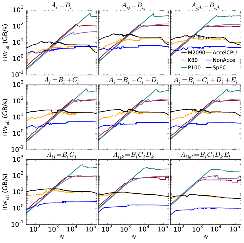
Figure 2: TLoops performance benchmarks of assignment (top row), addition (middle), and outer products (bottom). Operations increase in complexity as panels move from left to right. Each panel shows the effective bandwidth of the automatically generated GPU code (labelled by the GPU used for the benchmarks), automatically generated CPU code (AccelCPU), and expression templates without automatic code generation (NonAccel). The black line (SpEC) shows the performance of SpEC without the use of the TLoops package.

Let us now discuss and interpret Figure 2. Focusing first on the GPUs, ‘M2090’, ‘K80’, and ‘P100’ all show the same overall trends. Execution time is roughly constant in the gridsize until occupancy is saturated, after which point it increases linearly. Since the number of memory transactions increases linearly in gridsize throughout, $\mathrm{BW}_{\mathrm{eff}}$ shows linear increase up to the point of saturation, after which point it is constant. Since all the GPUs have essentially the same single-thread performance, they perform essentially identically until their respective points of saturation. However, newer cards (especially the P100) can support more parallel threads, resulting in a later point of saturation with a higher BW_eff.

The saturation gridsize is most importantly determined by the left-hand side tensor rank: higher rank tensors saturate earlier. For example, in Figure 2 the saturation gridsizes are almost identical for $A_{ij}=B_{ij}$ compared with $A_{ij}=B_{i}C_{j}$, for $A_{ijk}=B_{ijk}$ compared with $A_{ijk}=B_{i}C_{j}D_{k}$, and for $A_{i}=B_{j}$ compared with any of the addition operations Eqs. (13)-(15). This reflects our code’s parallelism over tensor indices, which is crucial for achieving good performance at gridsizes on the order of $10^{4}$. The pattern would not persist past rank 4 or for symmetric indices, since we serialize in these cases. Post-saturation performance is mostly independent of the operation and usually quite close - slightly beneath a factor of $2$ in the worst case of $A_{ijkl}=B_{i}C_{j}D_{k}E_{l}$ - to the measured bandwidths from bandwidthTest.

In contrast, the three CPU execution-paths do not suffer from high latency, and so the BW_eff curves are generally quite flat with respect to gridsize. Nevertheless, several patterns are visible in the relative exeuction speed of the three CPU execution paths. Except sometimes for assignments (Eqs. (10)-(12)) at very large gridsize, the expression-template code (NonAccel) usually gives worse performance than either the automatically-generated C code (AccelCPU) or that SpEC without any TLoops simplifications (SpEC) by a factor of between about 3-10. These results are roughly in line with those obtained from Walter Landry’s FTensor [2, 8], which is similar to TLoops running in NonAccel mode, and is presumably due to the compiler being less able to optimize the various templated expression templates.

More unexpectedly, SpEC and AccelCPU do not perform identically. While performance is usually comparable, SpEC is sometimes noticeably superior, especially for less complex operations at small gridsizes. AccelCPU differs from SpEC in two ways. First, the for loops over tensor indices appear directly in source code using SpEC, whereas AccelCPU routes through a few extra classes before reaching them. While we consider it unlikely, the impaired performance for less complex operations may be due to some extra overhead from this routing. Second, SpEC handles the loop over gridpoints using expression templates, while AccelCPU uses an additional for loop. This may result in differing behaviour regarding e.g. the creation of temporaries and the use of cached memory in the machine code.

Now comparing the performance of the GPUs with the CPU executions paths, we note that the CPU generally gives better performance at small gridsize, but is eventually surpassed by the GPU. This is the expected behaviour: the CPU has superior single-thread performance, but the GPU has more capacity for paralellism. Compiler optimizations available to the CPU will likely also result in more efficient reuse of memory than on the GPU. This will make operations on the CPU less complex, but also make the floating-point performance of the hardware more relevant. Thus, the CPU has less of an advantage at small gridsize for more computationally intensive operations.

5.3 Benchmarks of more complex expressions

Let us now turn to the more complex operations corresponding to Eqs. (LABEL:eq:Contract1)-(21), Eq. (6), and the GH equations, each described in Section 5.1. We proceed here as in Section 5.2, benchmarking six hardware and code-execution-path combinations as a function of gridsize, with results presented in Figure 3.

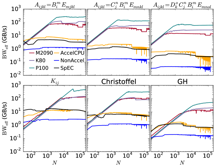
Figure 3: TLoops performance benchmarks of contraction (top row) and of practical numerical relativity operations (bottom). Each panel is formatted in the same way as in Figure 2. The leftmost and central operations in the bottom panel correspond respectively to Equations 21 and 6. The rightmost operation, “GH”, shows the performance of the entire SpEC module that advances the Einstein equations (in their generalized harmonic formulation) by a timestep.

Figure 3 shows broadly similar features throughout: GPU performance increases linearly up to a saturation point and then is constant, while CPU performance is nearly flat. In particular, the $K_{\mathrm{ij}}$ operation (Eq. (21), lower left panel of Figure 3) behaves essentially identically to Eq. (17) (lower left panel of Figure 2), to which it is indeed very similar in form.

The contraction operations (Eqs. (LABEL:eq:Contract1), (19), and (20)) in the top row of Figure 3 show some new behaviour. On the CPU, we first of all notice that performance, while still independent of gridsize, worsens sharply as we move from left to right between panels. These operations are more strongly compute-bound than those discussed until now, although the form of our automatically generated code does not expose this. Since the CPU performs memory operations relatively better than floating-point computations, its performance degrades for operations involving more of the latter.

We also notice that AccelCPU gives better performance than does SpEC for these operations, which is the opposite behaviour as observed previously. We can only guess at the reason for this. Perhaps there is more opportunity for compiler optimizations for operations involving more floating-point operations, but the expression-templates over gridsize used by SpEC prevent those optimizations from being made.

Turning attention to the GPU curves, we see that the low-gridsize performance is almost exactly identical between panels. Due to the massive parallelism it must support, the CUDA compiler cannot make nearly so aggressive optimizations as can a modern C++ compiler, and so the automatically-generated code presumably behaves in the bandwidth-bound manner in which it is written. The saturation gridsize, however, does change, even though the number of LHS indices remains constant. Similarly, the post-saturation performance gets lower as we move from left to right.

This stems from the fact that the SpEC class Tensor is a list of arrays (one array over the spatial grid per tensor index), rather than a single contiguous one. Since the tensors are not contiguous each memory access actually involves two pointer indirections, one each to retrieve the appropriate component array and spatial gridpoint. For example an instruction such as d = A[i][j][x] must first load A[i] from global memory, then A[i][j], then finally A[i][j][x]. Since the first two loads are not in principle necessary, we do not include them in the numerator of $\mathrm{BW}_{\mathrm{eff}}$. Since that numerator therefore underestimates the true number of memory transactions our computed $\mathrm{BW}_{\mathrm{eff}}$ will be correspondingly lower.

	M2090		K80		P100
Operation	Regs	% Occ	Regs	% Occ	Regs	% Occ
(10)	10	100	10	93.8	12	93.8
(11)	10	100	10	93.8	12	93.8
(12)	10	83.3	10	93.8	12	93.3
(13)	14	100	14	93.8	14	93.8
(14)	18	100	16	93.8	15	93.8
(15)	20	100	21	93.8	18	93.8
(16)	14	100	14	93.8	14	93.8
(17)	18	83.3	16	93.8	16	93.8
(18)	21	83.3	21	93.8	18	93.8
(LABEL:eq:Contract1)	28	72.9	29	93.8	24	93.8
(19)	38	41.7	42	93.8	32	93.8
(20)	50	41.7	56	93.8	48	62.5
(21)	21	87.5	42	93.8	32	93.8
(6)	34	62.5	32	93.8	32	93.8

Table 2: Per-thread register count (Regs) and theoretical occupancy (% Occ) for benchmarked TLoops operations on each GPU as measured by the NVIDIA visual profiler. On the M2090, K80, and P100, register use begins to impair occupancy respectively at counts exceeding 21, 64, and 32. The GH operation is not profiled here since it does not consist of a single kernel.

The extra indirections also result in additional thread latency, since the thread must stall between the successive loads, and since the large number of loads may exhaust the SMs memory pipeline. This last effect could in principle be alleviated by staggering loads to avoid memory dependency, but this would complicate automatic code generation considerably. Future improvements will instead focus on making tensors contiguous.

The extra pointers finally result in extra thread-local memory allocations, increasing the kernel’s per-thread register count. Each streaming multiprocessor (SM) in a GPU has physically a single register file that is logically allocated to threads as needed. Each SM is also theoretically capable of simultaneously executing a certain number of warps, each consisting of 32 threads, but only if the per-thread register count is small enough that these warps do not collectively exhuast the register file.

On the M2090, K80, and P100 respectively, this occurs when the per-thread register count exceeds 21, 64, and 32. The SMs on the K80 and P100 have equally sized register files (of 256kb, compared to 128kb on the M2090), but the P100 SMs can also potentially execute more warps, resulting in a lower register threshold for maximum occupancy. If the limit is saturated by a large threshold, occupancy will significantly decrease, resulting in an earlier point of saturation with worse asymptotic performance. We never exceed this threshold on the K80 (Table 2) but it does sometimes become relevant for operations involving contractions.

Finally, let us turn attention to the GH operation, in the lower right panel of Figure 3. On the GPU, the transition from linear to constant performance growth is not nearly so sharp as for the single-expression operations. This presumably reflects an averaging out between the many saturation points of the differing expressions within GH. GH also displays (in all cases) noticeably worse performance compared to its predecessors in this discussion. The GH operation consists of many succcessive individual kernels, many of which are complex contractions; thus, the above discussion of contractions applies here as well. On top of this, the many individual kernel launches add latency to the GPU execution time.

5.4 Impact of CPU compiler

In Figure 4, we show some benchmarks illustrating the relative performance of gcc vs. Intel compilers operating upon our code. Generically, but not always, gcc gives better performance. The difference is most stark for the C++11 expression templates of NonAccel, which work over an order of magnitude faster using gcc throughout. gcc also gets uniformly better performance out of the AccelCPU code, though the difference is less dramatic. Without TLoops (“SpEC”), the compilers do behave differently, but their relative performance varies between operations.

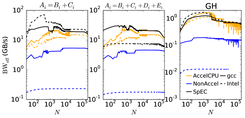
Figure 4: TLoops performance of selected operations illustrating the respective performance of the CPU code when compiled using gcc (solid lines) vs Intel (dashed) compilers. The detailed version and compiler arguments are given in Section 5 of the text. Formatting is otherwise identical to Figures 2 and 3.

5.5 Impact of templating over Tensor-indices

From the perspective of automatic GPU-porting, an alternative approach to TLoops would be to automatically generate code from SpEC’s existing spatial-gridpoint expression templates. For example, in Listing 4, one might automatically generate code only for the interior operation, and not for the full expression including the for loops over i and j. This would be much simpler to write, and would require no source code modifications at all.

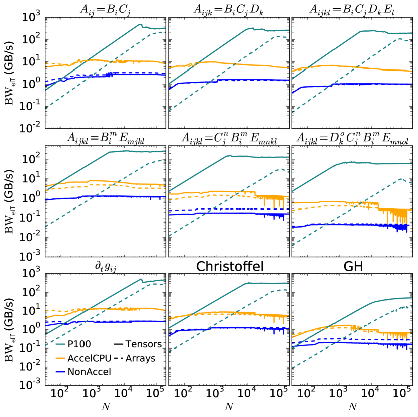
Figure 5: TLoops performance of selected operations showing the performance advantage attained by templating over entire tensors (solid lines, “Tensors” in the legend) rather than individual component arrays (dashed lines, “Arrays”). These plots are otherwise formatted in the same way as in Figures 2 and 3. To avoid visual confusion we display results from only one GPU (the P100), but the qualitative behaviour is the same for each.

Chronologically, this approach was the first we tried. TLoops was motivated by its strongly negative performance impact on the SpEC code proper. The performance decrease accounting for this is illustrated in Figure 5. Here, we benchmark various expressions using the P100 GPU and the two TLoops CPU execution pathways. For the lines marked Tensors, TLoops is used to represent the full expression, as in Listing 2. For those marked Arrays, it is used only to represent operations over individual Tensor elements, which therefore are surrounded by explicit for loops in source code, as in Listing 1. While the respective performance of the two strategies is comparable on the CPU, on the GPU TLoops expressions are vastly superior, particularly at realistic gridsizes between about $1000$ and $60000$.

Templating over tensor indices is advantageous on the GPU for three reasons. First, launching a GPU kernel carries an overhead of about 20 $\mu$ s. In the array loop approach this overhead needs to be paid once per every free and contracted index in the operation. Automatically ported operations will usually be small, and in practice launch overhead is very often the dominant expense. A TLoops operation, on the other hand, launches only one kernel. Second, TLoops operations are paralellized over the left-hand side tensor indices as well as the spatial grid, whereas the array loop approach can parallelize only over the spatial grid. In principle the array loop approach could achieve some index-level parallelism via concurrent execution of GPU kernels. However, the aforementioned launch overhead synchronizes the device, preventing concurrent execution in practice.

6 Conclusion

We have presented a software package, TLoops, which allows tensor-algebraic expressions to compile and execute in C++ code. TLoops can also automatically generate equivalent C++ or CUDA code to these expressions, which can be linked back to a second compilation. We have shown this automatically generated code to give identical or comparable performance compared to the code SpEC uses by default, and that the CUDA code often outperforms the CPU. Even at only moderate gridsizes of a few 1000, the CUDA code often comes close to the peak (memory-bound) performance of the GPU.

Significant opportunity remains for improvement. The code at present is intertwined with the rest of SpEC. We hope to separate it from the latter into an independent open-source library. Opportunity for performance improvements also exists. In particular, we are working on adopting a contiguous Tensor class within SpEC. This will allow for simpler, faster automatic code.

We hope the simplifications to coding effort made possible by TLoops may speed the development of future code, inside and outside of numerical relativity.

7 Conflicts of Interest

The authors have no conflicts of interest to report.

8 Acknowledgments

We thank Nils Deppe and Mark Scheel for helpful discussions. Calculations were performed with the SpEC-code [1]. We gratefully acknowledge support from NSERC of Canada, form the Canada Research Chairs Program, and from the Canadian Institute for Advanced Research. Some calculations were performed at the SciNet HPC Consortium [10]. SciNet is funded by: the Canada Foundation for Innovation (CF) under the auspices of Compute Canada; the Government of Ontario; Ontario Research Fund (ORF) – Research Excellence; and the University of Toronto.

References

- SpE [e0cm] http://www.black-holes.org/SpEC.html, .
- Landry [2012] W. Landry, Implementing a high performance tensor library, http://www.wlandry.net/Presentations/FTensor.pdf, 2012.
- Arndt et al. [2017] D. Arndt, W. Bangerth, D. Davydov, T. Heister, L. Heltai, M. Kronbichler, M. Maier, J.-P. Pelteret, B. Turcksin, D. Wells, The deal.II library, version 8.5, Journal of Numerical Mathematics (2017).
- jer [1998] Tensor objects in finite element programming, International Journal for Numerical Methods in Engineering 41 (1998) 113–126.
- Reynders and Cummings [1998] J. V. Reynders, III, J. C. Cummings, The pooma framework, Comput. Phys. 12 (1998) 453–459.
- Tisdale [1999] R. Tisdale, Svmt, http://www.netwood.net/~edwin/svmt/, 1999.
- Veldhuizen [1996] T. Veldhuizen, Blitz++, http://www.oonumerics.org/blitz, 1996.
- FTe [2012] http://www.wlandry.net/Projects/FTensor#Benchmarks, 2012.
- Gamma et al. [1994] E. Gamma, R. Helm, R. Johnson, J. Vlissides, Design Patterns: Elements of Reusable Object-Oriented Software, Addison-Wesley Professional Computing Series, Pearson Education, 1994. URL: https://books.google.ca/books?id=6oHuKQe3TjQC.
- Loken et al. [2010] C. Loken, D. Gruner, L. Groer, R. Peltier, N. Bunn, M. Craig, T. Henriques, J. Dempsey, C.-H. Yu, J. Chen, L. J. Dursi, J. Chong, S. Northrup, J. Pinto, N. Knecht, R. V. Zon, SciNet: Lessons Learned from Building a Power-efficient Top-20 System and Data Centre, J. Phys.: Conf. Ser. 256 (2010) 012026.