Format Abstraction for Sparse Tensor Algebra Compilers

Abstract.

This paper shows how to build a sparse tensor algebra compiler that is agnostic to tensor formats (data layouts). We develop an interface that describes formats in terms of their capabilities and properties, and show how to build a modular code generator where new formats can be added as plugins. We then describe six implementations of the interface that compose to form the dense, CSR/CSF, COO, DIA, ELL, and HASH tensor formats and countless variants thereof. With these implementations at hand, our code generator can generate code to compute any tensor algebra expression on any combination of the aforementioned formats.

To demonstrate our technique, we have implemented it in the taco tensor algebra compiler. Our modular code generator design makes it simple to add support for new tensor formats, and the performance of the generated code is competitive with hand-optimized implementations. Furthermore, by extending taco to support a wider range of formats specialized for different application and data characteristics, we can improve end-user application performance. For example, if input data is provided in the COO format, our technique allows computing a single matrix-vector multiplication directly with the data in COO, which is up to 3.6$\times$ faster than by first converting the data to CSR.

1. Introduction

Tensor algebra is a powerful tool to compute on multidimensional data, with applications in machine learning (Abadi et al., 2016), data analytics (Anandkumar et al., 2014), physical sciences (Feynman et al., 1963), and engineering (Kolecki, 2002). Tensors generalize matrices to any number of dimensions and are often large and sparse, meaning most components are zeros. To efficiently compute with sparse tensors requires exploiting their sparsity in order to avoid unnecessary computations.

Recently, Kjolstad et al. (2017) proposed taco, a compiler for sparse tensor algebra. taco takes as input a tensor algebra expression in high-level index notation and generates efficient imperative code that computes the expression. Their compiler technique supports tensor operands stored in any format where each dimension can be described as dense or sparse. This encompasses tensors stored in dense arrays as well as variants of the compressed sparse row (CSR) format.

These are, however, only some of the tensor formats that are used in practice. Important formats that are not supported by taco include the coordinate (COO) format, the diagonal (DIA) format, the ELLPACK (ELL) format, and hash maps (HASH), along with countless blocked and high-dimensional variants and compositions of these. Each format is important for different reasons. COO is the natural way to enumerate sparse tensors and is often the format in which users provide data (Smith et al., 2017a). It is not the most performant format, but when a tensor will only be used once, it is often more efficient to compute directly with COO than to convert the data to another format. ELL exposes vectorization opportunities for SpMV and is useful for matrices that contain a bounded number of nonzeros per row, such as matrices from well-formed meshes. DIA has the added benefit of being very compact and is suited to matrices that compute stencils on Eulerian grids and images. Hash maps support random access without having to explicitly store zeros and can be useful for multiplications involving very sparse operands. An application may need any, or even several, of these formats, making it important to support computing with all and any combination of them.

The approach of Kjolstad et al. (2017) was hard-coded for sparse dimensions that are compressed using the same arrays as CSR. By contrast, COO matrices store full coordinates, while DIA implicitly encodes coordinates of nonzeros using very different data structures. To enable efficiently computing with any format, a tensor algebra compiler must emit distinct code to cheaply iterate over each format. COO, for instance, needs a single loop that iterates over row and column dimensions together (Figure 1), whereas CSR needs two nested loops that each iterate over a dimension (Figure 1). To efficiently compute with operands in multiple formats, a compiler must emit code that concurrently iterates over the operands. Figure 1 shows, however, that this is not a straightforward combination of code that individually iterate over the operand formats. Rather, a compiler must also emit distinct code for each combination of formats to obtain good performance in all cases. Because the number of combinations is exponential in the number of formats though, one cannot readily extend the approach of Kjolstad et al. (2017) to support additional formats by directly hard-coding for them in the code generator. We instead need a different approach that is modular with respect to formats.

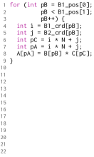
(a) $B$ is COO, $C$ is dense array

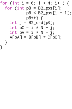
(b) $B$ is CSR, $C$ is dense array

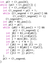
(c) $B$ is CSR, $C$ is COO

Figure 1. Code to compute the component-wise product of two matrices stored in varying formats.

We generalize the recent work on tensor algebra compilation to support a much wider range of disparate tensor formats. We describe a level-based abstraction that captures how to efficiently access data structures for encoding tensor dimensions, but that hides the specifics behind a fixed interface. We develop six per-dimension formats, all of which expose this common interface, that compose to express all the tensor formats mentioned above. Two of these per-dimension formats—dense and compressed—were hard-coded into taco. The other four—singleton, range, offset, and hashed—are new to this work and compose to express variants of COO, DIA, ELL, HASH, and countless other tensor formats not supported by Kjolstad et al. (2017). We then present a code generation algorithm that, guided by our abstraction, generates efficient tensor algebra kernels that are optimized for operands stored in any mix of formats. The result is a powerful system that lets users mix and match formats to suit their application and data, and which can be readily extended to support new formats without modifying the code generator. In summary, our contributions are:

Levelization:

We survey many known tensor formats (Section 2) and show that they can be represented as hierarchical compositions of just six per-dimension level formats (Figure 4).

Level abstraction:

We describe an abstraction for level formats that hides the details of how a level format encodes a tensor dimension behind a common interface, which describes how to access the tensor dimension and exposes its properties (Section 3).

Modular code generation:

We present a code generation technique that emits code to efficiently compute on tensors stored in any combination of formats, which reasons only about capabilities and properties of level formats and is not hard-coded for any specific format (Section 4).

To evaluate the technique, we implemented it as an extension to the taco tensor algebra compiler (Kjolstad et al., 2017). We find that our technique emits code that has performance competitive with existing sparse linear and tensor algebra libraries. Our technique also supports a much wider range of sparse tensor formats than other existing libraries as well as the approach of Kjolstad et al. (2017). This lets us improve the end-to-end performance of applications that use taco. For instance, our extension enables computing a single matrix-vector multiplication directly with data provided in the COO format, which is up to 3.6$\times$ faster than by first converting the data to CSR (Section 5).

2. Tensor Storage Formats

There exist many formats for storing sparse tensors that are used in practice. Each format is ideal under specific circumstances, but none is universally superior. The ideal format depends on the structure and sparsity of the data, the computation, and the hardware. It is thus desirable to support computing with as many formats as possible. This is, however, made difficult by the need for specialized code for every combination of operand tensor formats, even for the same computation.

2.1. Survey of Tensor Formats

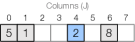
(a) An 8-vector

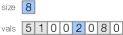
(b) Dense array

(c) Sparse vector

(d) Hash map

Figure 2. Identical tensors stored in various formats. Array elements shaded blue encode the same nonzero.

  (e) A 4$\times$6 matrix (f) COO (g) CSR (h) DCSR (i) ELL (j) DIA (k) BCSR (l) CSB   (m) A 3$\times$4$\times$2 tensor (n) COO (o) CSF (p) Mode-generic

Several examples of tensor storage formats from the literature are shown in Figure 2. A straightforward way to store an $n$th-order tensor (i.e., a tensor with $n$ dimensions) is to use an $n$-dimensional dense array, which explicitly stores all tensor components including zeros. Figure 2 shows dense storage for an 1st-order tensor (a vector). A desirable feature of dense arrays is that the value at any coordinate can be accessed in constant time. Storing a sparse tensor in a dense array, however, is inefficient as a lot of memory is wasted to store zeros. Furthermore, performance is lost computing with these zeros even though they do not meaningfully contribute to the result. For tensors with many large dimensions, it may even be impossible to use a dense array due to lack of memory.

The simplest way to efficiently store a sparse tensor is to keep a list of its nonzero coordinates and values (Figures 2,  2, and 2). This is typically known as the coordinate (COO) format (Bader and Kolda, 2007). In contrast to dense arrays, COO tensors consume only $\Theta(\operatorname{nnz})$ memory. In addition, many common file formats for storing tensors, such as the Matrix Market exchange format (National Institute of Standards and Technology, 2013) and the FROSTT sparse tensor format (Smith et al., 2017a), closely mirror the COO format. This minimizes preprocessing cost as inserting nonzero values and their coordinates only requires appending them to the crd and vals arrays.

Unlike dense arrays though, the COO format does not provide efficient random access. This, as we will see in Section 4, limits the performance of multiplicative operations. Hash maps (HASH) eliminate this drawback by storing tensor coordinates in a randomly accessible hash table (Figure 2). However, hash maps do not support efficiently iterating over stored nonzeros in order, which in turn restricts the performance of additive operations.

The COO format also redundantly stores row coordinates that are compressed out in the compressed sparse row (CSR) format for sparse matrices/2nd-order tensors (Figure 2). Compressing out redundant row coordinates increases performance for computations that are typically memory bandwidth-bound, such as sparse matrix-vector multiplication (SpMV). In Figure 2, for instance, the row coordinate is duplicated for the last three nonzeros in the same row. CSR removes the redundant row coordinates, using an auxiliary array (pos in Figure 2) to keep track of which nonzeros belong to each row. The doubly compressed sparse row (DCSR) format (Buluç and Gilbert, 2008) achieves additional compression for hypersparse matrices by only storing the rows that contain nonzeros (Figure 2). For higher-order tensors, Smith and Karypis (2015) describe a generalization of CSR, called compressed sparse fiber (CSF), that compresses every dimension (Figure 2). Tensors stored in any of these compressed formats, however, are costly to assemble or modify.

Many important applications work with tensors whose nonzero components form a regular pattern. Matrices that encode vertex-edge connectivity of well-formed unstructured meshes, for instance, have a bounded number of nonzero components per row. This is exploited by the ELLPACK (ELL) format, which stores the same number of components for each row (Figure 2) (Kincaid et al., 1989). Thus, it only has to store the column coordinates and nonzero values in the implicitly indexed row positions, which are stored contiguously in memory making it possible to efficiently vectorize SpMV (D’Azevedo et al., 2005). If nonzeros are further restricted to a few dense diagonals, then their coordinates can be computed from the offsets of the diagonals. This pattern is common in grid and image applications, and allows the diagonal (DIA) format to forgo storing the column coordinates altogether (Figure 2) (Saad, 2003). However, for matrices that do not conform to assumed structures, structured tensor formats may needlessly store many zeros and thus actually degrade performance.

The block compressed sparse row (BCSR) format (Im and Yelick, 1998) generalizes CSR by storing a dense block of nonzeros in the vals array for every nonzero coordinate (Figure 2). This reduces storage and exposes opportunities for vectorization, and is ideal for inherently blocked matrices from FEM applications. The mode-generic sparse tensor format, proposed by Baskaran et al. (2012), generalizes the idea of BCSR to higher-order tensors (Figure 2). It stores a tensor as a sparse collection of any-order dense blocks, with the coordinates of the blocks stored in COO (i.e., the crd arrays). By contrast, the compressed sparse block (CSB) format, proposed by Buluç et al. (2009), represents a matrix as a dense collection of sparse blocks stored in COO (Figure 2).

2.2. Computing with Disparate Tensor Formats

The existence of so many disparate tensor formats makes it challenging to support efficiently computing with all of them. As we have seen, different formats may use vastly dissimilar data structures to encode tensor coordinates and thus need very different code to iterate over them. Iterating over a dense matrix’s column dimension, for instance, simply entails looping over all possible coordinates along the dimension. Efficiently iterating over a CSR matrix’s column dimension, by contrast, requires looping over its crd array and dereferencing it at each position to access the column coordinates (Figure 1, lines 2–5). Furthermore, to efficiently compute with tensors stored in different combinations of formats can require completely different strategies for simultaneously iterating over multiple formats. For example, code to compute the component-wise product of CSR matrix $B$ with dense matrix $C$ simply has to iterate over $B$ and pick out corresponding nonzeros from $C$ (Figure 1, line 6). Computing the same operation with COO matrix $C$, however, requires vastly different code as neither CSR nor COO supports efficient random access into the column dimension. Instead, code to compute the component-wise product has to simultaneously co-iterate over and merge the crd arrays that encode $B$ and $C$’s column coordinates (Figure 1, lines 8–20).

To obtain good performance with all tensor formats, a code generator therefore needs to be able to emit specialized code for any combination of distinct formats. The approach of Kjolstad et al. (2017) manages this by effectively hard-coding a distinct strategy for computing with each format combination into the code generator. (More precisely, it hard-codes for combinations of the two formats that may be used to encode tensor dimensions.) However, this approach does not scale with the number of supported formats. In particular, let $F$ denote a set of formats that use distinct data structures to encode nonzeros. Each subset of $F$ represents a combination of distinct formats that can be used to store operands in a tensor algebra expression. Supporting all formats in $F$ would thus require individually hard-coding a code generation strategy for every subset of $F$, of which there are $\Theta(2^{|F|})$. This exponential blow-up effectively prevented taco from supporting more disparate tensor formats like COO and DIA, necessitating a more scalable solution.

3. Tensor Storage Abstraction

As we have seen, a tensor algebra compiler must generate specialized code for every possible combination of supported formats in order to obtain good performance. Since the number of combinations is exponential in the number of formats though, it is infeasible to exhaustively hard-code support for every possible format. In this section, we show how common variants of all the tensor formats examined in Section 2 can be expressed as compositions of just six per-dimension formats. We will also present an abstraction that captures shared capabilities and properties of per-dimension formats. The abstraction generalizes common patterns of accessing tensor storage and guides a format-agnostic code generation algorithm that we describe in Section 4.

3.1. Coordinate Hierarchies

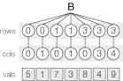
(a) COO

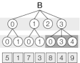
(b) CSR

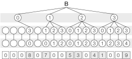
(c) DIA

Figure 3. Coordinate hierarchies for the same matrix, shown in Figure 2, stored in different formats. The levels labeled rows and cols encode the matrix’s row and column coordinates respectively. A coordinate hierarchy’s structure reflects how the underlying storage format encodes a tensor’s nonzeros.

The per-dimension formats can be understood by viewing tensor storage as a hierarchy of coordinates, where each hierarchy level encodes the coordinates along one tensor dimension. Each path from the root to a leaf in this hierarchy encodes the coordinates in each dimension of one tensor component. Figure 3 shows examples of coordinate hierarchies for a matrix stored in different formats. The matrix component values are shown at the bottom of each hierarchy. In Figure 3, for instance, the rightmost path represents the tensor component $B(3,4)$ with the value $9$. As we will see in Section 4, representing tensor storage hierarchically lets a code generator decompose any computation into the simpler problem of merging coordinate hierarchy levels.

The structure of a coordinate hierarchy reflects the encoding of nonzeros in memory and lets the code generator reason about how to iterate over tensors without knowing the specific tensor format. For example, the coordinate hierarchy for a COO matrix (Figure 3) consists of coordinate chains that encode each nonzero. This chain structure reflects that the COO format stores the complete coordinates of each nonzero. By contrast, the coordinate hierarchy for a CSR matrix (Figure 3) is tree-structured and components in the same row share a row coordinate parent. This tree structure reflects that the CSR format removes redundant row coordinates using the auxiliary pos array.

A coordinate hierarchy has one level (shaded light gray in Figure 3) for every tensor dimension, and per-dimension level formats describe how to store coordinate hierarchy levels in memory. Each position (a node) in a level may encode some coordinate (the number in the node) along the corresponding tensor dimension. Alternatively, a position may contain an unlabeled node, which encodes no coordinate and reflects padding in the underlying physical storage. The unlabeled nodes in Figure 3, for instance, represent segments of each diagonal that are out of the bounds of valid matrix coordinates. Typically, different levels in a coordinate hierarchy will be stored in separate data structures in memory, though the abstraction also permits levels to share the same underlying data structure. As will be evident, this can be useful for some tensor formats such as DIA, which uses the same array (i.e., offset) to encode both the row and column levels in Figure 3.

Each node in a level may also be connected to a parent in the previous level. Coordinates that share the same parent are referred to as siblings. The coordinates highlighted in dark gray in Figure 3, for instance, are siblings that share the parent row coordinate $3$. A coordinate’s ancestors refer to the set of coordinates that are encoded by the path from its parent to the root.

We propose six level formats that suffice to represent all the tensor formats described in Section 2, though many more are possible within our framework. Each level format (or level type) can encode all the nodes in a level along with the edges connecting them to their parents. Some of these level formats implicitly encode coordinates (e.g., as an interval), while others explicitly store them (e.g., in a segmented vector). At a high level, given a parent coordinate in the $(i-1)$-th level of a coordinate hierarchy, the six level formats encode its children coordinates in the $i$-th level as follows:

Dense:

levels store the size of the corresponding dimension ($N$) and encode the coordinates in the interval $[0,N)$. Figure 3 shows the row dimension of a CSR matrix encoded as a dense level with the array on the right.

Compressed:

levels store coordinates in a segment of the crd array, with the segment bounds stored in the pos array. Figure 3 shows the column dimension of a CSR matrix encoded as a compressed level with the arrays on the right. Given a parent coordinate 1, for instance, the level encodes two child coordinates 0 and 1, stored in crd between positions $\texttt{pos[1]}=2$ (inclusive) and $\texttt{pos[2]}=4$ (exclusive).

Singleton:

levels store a single coordinate with no sibling in the crd array. Figure 3 shows the column dimension of a COO matrix encoded as a singleton level with the array on the right.

Range:

levels encode the coordinates in an interval with bounds computed from an offset and from dimension sizes $N$ and $M$. Figure 3 shows the row dimension of a DIA matrix encoded as a range level with the arrays on the right. Given a parent coordinate 1, the level encodes coordinates between $\max(0,-\texttt{offset[1]})=1$ and $\min(4,6-\texttt{offset[1]})=4$.

Offset:

levels encode a single coordinate with no sibling, shifted from the parent coordinate by a value in the offset array. Figure 3 shows the column dimension of a DIA matrix encoded as an offset level with the array on the right. Given a parent coordinate 3 and an offset index 1, for instance, the level encodes the coordinate $3+\texttt{offset[1]}=2$.

Hashed:

levels store coordinates in a segment, of size $W$, of a hash map (crd). The arrays on the right, with empty buckets marked by $-1$, encode the column dimension of a hash map row vector as a hashed level.

Table 2 presents the precise semantics of the level formats, encoded in level functions that each level format implements and that fully describe how data structures associated with the level format can be interpreted as a coordinate hierarchy level. (Section 3.2 describes level functions in more depth.) Figure 4 shows how these level formats can be composed to express all the tensor formats surveyed in Section 2. The same level formats, however, may be combined in other ways to express additional tensor formats. For instance, a variant of DIA for matrices that have only sparsely-filled diagonals can be expressed as the combination (dense, compressed, offset), which replaces the range level that implicitly assumes diagonals are densely filled. We cast structured matrix formats, like BCSR, as formats for higher-order tensors; the added dimensions expose more complex tensor structures.

(a) Vector storage formats

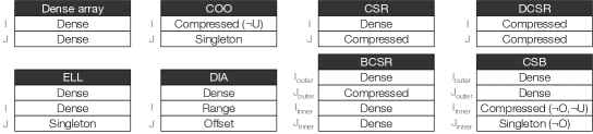
(b) Matrix storage formats

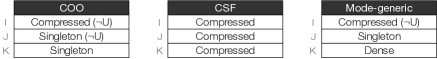
(c) 3rd-order tensor storage formats

Figure 4. Common tensor formats composed from per-dimension level formats. We cast structured matrix formats as higher-order tensor formats. The label beside a level identifies the tensor dimension it represents. Unless otherwise stated, all levels other than hashed are ordered and unique (see Section 3.3); hashed levels are unordered and unique. ($\neg$O) denotes an unordered level and ($\neg$U) denotes a non-unique level.

The code generator in Section 4 emits code that accesses and modifies coordinate hierarchy levels through an abstract level interface, which ensures the code generator is not tied to specific formats. This makes it extensible and maintainable as adding support for new formats does not require any change to the code generation algorithm. The abstract interface to a coordinate hierarchy level consists of level capabilities and properties. Level capabilities instruct the code generator on how to iterate over and index into levels, as well as on how to add coordinates to a level. Properties of a level let the compiler emit optimized loops that exploit tensor attributes to increase computational performance. Table 1 identifies the capabilities and properties of each level type.

Table 1. Supported capabilities and properties of each level type. V, P, I, and A indicate that a level type supports coordinate value iteration, coordinate position iteration, insert, and append respectively. A (✓) indicates that a level type can be configured to either possess or not possess a particular property.

Level Type	Capabilities			Properties
	Iteration	Locate	Assembly	Full	Ordered	Unique	Branchless	Compact
Dense	V	✓	I	✓	(✓)	(✓)		✓
Range	V				(✓)	(✓)
Compressed	P		A	(✓)	(✓)	(✓)		✓
Singleton	P		A	(✓)	(✓)	(✓)	✓	✓
Offset	P				(✓)	(✓)	✓
Hashed	P	✓	I	(✓)		(✓)

3.2. Level Access Capabilities

Every coordinate hierarchy level provides a set of capabilities that can be used to access or modify its coordinates. Each capability is exposed as a set of level functions with a fixed interface that a level must implement to support the capability. Table 1 identifies the capabilities that each level format supports, and Table 2 shows the level functions that implement the access capabilities.

Level capabilities provide an abstraction for manipulating physical indices (tensor storage) in a format-agnostic manner. As an example, the column dimension of a CSR matrix is a compressed level, which provides the coordinate position iteration capability. This capability is exposed as two level functions, pos_bounds and pos_access, as shown in Table 2. To access the column coordinates in dark gray in Figure 3, we first determine their range by calling pos_bounds with the position of row coordinate 3 as input. We then call pos_access for each position in this range to get the column coordinate values. Under the hood, pos_bounds indexes the pos array to locate the crd array segment that stores the column coordinates, while pos_access retrieves each of the coordinates from crd. These level functions fully describe how to access CSR indices efficiently, while hiding details such as the existence of the pos and crd arrays from the caller.

The abstract interface to a coordinate hierarchy level exposes three different access capabilities: coordinate value iteration, coordinate position iteration, and locate. Every level must provide coordinate value iteration or coordinate position iteration and may optionally also provide the locate capability. Table 1 identifies the access capabilities supported by each level type. Our code generation algorithm will emit code that calls level functions to access physical tensor storage, which ensures the algorithm is not tied to any specific types of data structures.

Table 2. Level functions defined for each of the six level types listed in Section 3.1. Section 3.2 describes how these level functions implement the access capabilities supported by each level type, as identified in Table 1.

Level Type	Level Function Definitions
Dense	⬇ coord_bounds(i1, $\dots$, ik-1): return <0, Nk>	⬇ coord_access(pk-1, i1, $\dots$, ik): return <pk-1 * Nk + ik, true>
	⬇ locate(pk-1, i1, $\dots$, ik): return <pk-1 * Nk + ik, true>
Range	⬇ coord_bounds(i1, $\dots$, ik-1): return <max(0, -offset[ik-1]), min(Nk, Mk - offset[ik-1])>	⬇ coord_access(pk-1, i1, $\dots$, ik): return <pk-1 * Nk + ik, true>
Compressed	⬇ pos_bounds(pk-1): return <pos[pk-1], pos[pk-1 + 1]>	⬇ pos_access(pk, i1, $\dots$, ik-1): return <crd[pk], true>
Singleton	⬇ pos_bounds(pk-1): return <pk-1, pk-1 + 1>	⬇ pos_access(pk, i1, $\dots$, ik-1): return <crd[pk], true>
Offset	⬇ pos_bounds(pk-1): return <pk-1, pk-1 + 1>	⬇ pos_access(pk, i1, $\dots$, ik-1): return <ik-1 + offset[ik-2], true>
Hashed	⬇ pos_bounds(pk-1): return <pk-1 * Wk, (pk-1 + 1) * Wk>	⬇ pos_access(pk, i1, $\dots$, ik-1): return <crd[pk], crd[pk] != -1>
	⬇ locate(pk-1, i1, $\dots$, ik): int pk = ik % Wk + pk-1 * Wk if (crd[pk] != ik && crd[pk] != -1) { int end = pk do { pk = (pk + 1) % Wk + pk-1 * Wk } while (crd[pk] != ik && crd[pk] != -1 && pk != end) } return <pk, crd[pk] == ik>

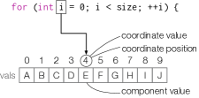
(a) Iterating over a dense array

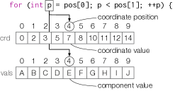
(b) Iterating over a sparse vector

⬇

ibegin_k, iend_k = coord_bounds(i₁, $...$, i_k-1);

for (i_k = ibegin_k; i_k < iend_k; ++i_k) {

p_k, found = coord_access(p_k-1, i₁, $...$, i_k);

if (found) {

// coords and values dominated by i$\color[rgb]{.5,.5,.5}_{k}$ at pos

// p$\color[rgb]{.5,.5,.5}_{k}$ encode subtensor $\color[rgb]{.5,.5,.5}B(i_{1},...,i_{k},:,...,:)$

}

}

(c) Coordinate value iteration

⬇

pbegin_k, pend_k = pos_bounds($p_{k-1}$);

for (p_k = pbegin_k; p_k < pend_k; ++p_k) {

i_k, found = pos_access(p_k, i₁, $...$, i_k-1);

if (found) {

// coords and values dominated by i$\color[rgb]{.5,.5,.5}_{k}$ at pos

// p$\color[rgb]{.5,.5,.5}_{k}$ encode subtensor $\color[rgb]{.5,.5,.5}B(i_{1},...,i_{k},:,...,:)$

}

}

(d) Coordinate position iteration

Figure 5. To iterate over a dense vector, we loop over its coordinates and use them to index into the vals array. To iterate over a sparse vector, we loop over coordinate positions and use them to access the crd and vals arrays. Coordinate value iteration and coordinate position iteration generalize these patterns.

Coordinate Value Iteration

The coordinate value iteration capability directly iterates over coordinates. It generalizes the method in Figure 5 for iterating over a dense vector and is exposed as two level functions. The first returns an iterator over coordinates of a coordinate hierarchy level (coord_bounds) and the second accesses the position of each coordinate (coord_access):

⬇

coord_bounds(i₁, $\dots$, i_k-1) -> <ibegin_k, iend_k>

coord_access(p_k-1, i₁, $\dots$, i_k) -> <p_k, found>

More precisely, given a list of ancestor coordinates ($i_{1},\dots,i_{k-1}$), coord_bounds returns the bounds of an iterator over coordinates that may have those ancestors. For each coordinate $i_{k}$ within those bounds, coord_access either returns the position of a child of $p_{k-1}$ that encodes $i_{k}$ and returns found as true, or alternatively returns found as false if the coordinate does not actually exist. These functions can be used to iterate tensor coordinates in the general case as demonstrated in Figure 5. In practice though, the code in  Figure 5 can be optimized by removing the conditional if we know that an implementation of coord_access always returns found as true.

Coordinate Position Iteration

The coordinate position iteration capability, on the other hand, iterates over coordinate positions. It generalizes the method in Figure 5 for iterating over a sparse vector and is also exposed as two level functions. The first returns an iterator over positions in a level (pos_bounds) and the second accesses the coordinate encoded at each position (pos_access):

⬇

pos_bounds(p_k-1) -> <pbegin_k, pend_k>

pos_access(p_k, i₁, $\dots$, i_k-1) -> <i_k, found>

More precisely, given a coordinate at position $p_{k-1}$, pos_bounds returns the bounds of an iterator over positions that may have $p_{k-1}$ as their parent. For each position $p_{k}$ in those bounds, pos_access returns the coordinate encoded at that position, or alternatively returns found as false if $p_{k}$ is not actually a child of $p_{k-1}$ or does not encode a coordinate (i.e., if $p_{k}$ is unlabeled). These functions can be used to iterate tensor coordinates with code like that shown in Figure 5; this code shares a similar structure to that for coordinate value iteration but has the roles of $i_{k}$ and $p_{k}$ reversed.

Locate

The locate capability provides random access into a coordinate hierarchy level through a function that computes the position of a coordinate:

⬇

locate(p_k-1, i₁, $\dots$, i_k) -> <p_k, found>

locate has similar semantics as coord_access. Given a coordinate $i_{k-1}$ at position $p_{k-1}$, locate attempts to locate among its children the coordinate $i_{k}$. If locate finds $i_{k}$, then it returns $i_{k}$’s position $p_{k}$ and returns found as true; otherwise it returns found as false. Traversing a path in a coordinate hierarchy to access a single tensor component can be done by successively calling locate at every level. As we will see in Section 4, having operands with efficient implementations of the locate capability leads to code that avoids iterating over every nonzero in those operands.

3.3. Level Properties

A coordinate hierarchy level may also declare up to five properties: full, ordered, unique, branchless, and compact. These properties describe characteristics of a level, such as whether coordinates are arranged in order, and are invariants that are explicitly enforced or implicitly assumed by the underlying physical index. The column dimension of a sorted CSR matrix, for instance, is both ordered and unique (Figure 4), which means it stores every coordinate just once and in increasing order. Our code generation technique relies on these level properties to emit optimized code.

Table 1 identifies the properties of each level type. Some coordinate hierarchy levels may be configured with a property, depending on the application. Configurable properties reflect invariants that are not tied to how a physical index encodes coordinates. For example, the crd array in compressed levels typically store coordinates in order when used in the CSR format, but the same data structure can also store coordinates out of order. Figure 4 shows how level types with configurable properties can be configured to represent tensor formats.

Full

A level is full if every collection of coordinates that share the same ancestors encompasses all valid coordinates along the corresponding tensor dimension. For instance, a level that represents a CSR matrix’s row dimension (Figure 3) encodes every row coordinate and is thus full. By contrast, a level that represents the same CSR matrix’s column dimension is not full as it only stores the coordinates of nonzero components.

Unique

A level is unique if no collection of coordinates that share the same ancestors contains duplicates. For example, a level that represents a CSR matrix’s row dimension necessarily encodes every coordinate just once and is thus unique. By contrast, a level that represents a COO matrix’s row dimension (Figure 3) can store a coordinate more than once and is thus not unique.

Ordered

A level is ordered if coordinates that share the same ancestors are ordered in increasing value, coordinates with different ancestors are ordered lexicographically by their ancestors, and duplicates are ordered by their parents’ positions. For example, a level that represents a sorted CSR matrix’s column dimension stores coordinates in increasing order and is thus ordered. A level that represents a hash map vector, however, is not as coordinates are stored in hash order instead.

Branchless

A level is branchless if no coordinate has a sibling and each coordinate in the previous level has a child. For example, the coordinate hierarchy for a COO matrix consists strictly of chains of coordinates, making the lower level branchless. By contrast, a level that represents a CSR matrix’s column dimension can have multiple coordinates with the same parent and is thus not branchless.

Compact

A level is compact if no two coordinates are separated by an unlabeled node that does not encode a coordinate. For instance, a level that represents a CSR matrix’s column dimension encodes coordinates in one contiguous range of positions and is thus compact. A level that represents a hash map vector, however, is not as it can have unlabeled positions that reflect empty buckets.

3.4. Level Output Assembly Capabilities

The capabilities described in Section 3.2 iterate over and access coordinate hierarchy levels. A level may also provide insert and append capabilities for adding new coordinates to the level. These capabilities let us assemble, in a format-agnostic manner, the data structures that store the result of a computation. Table 1 identifies the assembly capabilities that various level types support, and Table 3 shows the level functions that implement those capabilities.

Table 3. Definitions of level functions that implement assembly capabilities for various level types.

Level Type	Level Function Definitions
Dense	⬇ insert_coord(pk, ik): // do nothing	⬇ insert_init(szk-1, szk): // do nothing
	⬇ size(szk-1): return szk-1 * Nk	⬇ insert_finalize(szk-1, szk): // do nothing
Compressed	⬇ append_coord(pk, ik): crd[pk] = ik	⬇ append_init(szk-1, szk): for (int pk-1 = 0; pk-1 <= szk-1; ++pk-1) { pos[pk-1] = 0 }
	⬇ append_edges(pk-1, pbegink, pendk): pos[pk-1 + 1] = pendk - pbegink	⬇ append_finalize(szk-1, szk): int cumsum = pos[0] for (int pk-1 = 1; pk-1 <= szk-1; ++pk-1) { cumsum += pos[pk-1] pos[pk-1] = cumsum }
Singleton	⬇ append_coord(pk, ik): crd[pk] = ik	⬇ append_init(szk-1, szk): // do nothing
	⬇ append_edges(pk-1, pbegink, pendk): // do nothing	⬇ append_finalize(szk-1, szk): // do nothing
Hashed	⬇ insert_coord(pk, ik): crd[pk] = ik	⬇ insert_init(szk-1, szk): for (int pk = 0; pk < szk; ++pk) { crd[pk] = -1 }
	⬇ size(szk-1): return szk-1 * Wk	⬇ insert_finalize(szk-1, szk): // do nothing

Insert Capability

Inserts coordinates at any position and is exposed as four level functions:

⬇

insert_coord(p_k, i_k) -> void

size(sz_k-1) -> sz_k

⬇

insert_init(sz_k-1, sz_k) -> void

insert_finalize(sz_k-1, sz_k) -> void

The level function insert_coord inserts a coordinate $i_{k}$ into an output level at position $p_{k}$ given by locate, and requires that the level provide the locate capability. The level function insert_init initializes the data structures that encode an output level, while insert_finalize performs any post-processing required after all coordinates have been inserted. Both take, as inputs, the sizes of the level being initialized or finalized ($sz_{k}$) and its parent level ($sz_{k-1}$). For a level that provides the insert capability, its size is computed as a function of its parent’s size by the level function size. For a level that supports append, its size is the number of coordinates that have been appended.

Append Capability

Appends coordinates to a level and is also exposed as four level functions:

⬇

append_coord(p_k, i_k) -> void

append_edges(p_k-1, pbegin_k, pend_k) -> void

⬇

append_init(sz_k-1, sz_k) -> void

append_finalize(sz_k-1, sz_k) -> void

The level function append_coord appends a coordinate $i_{k}$ to the end of an output level ($p_{k}$). The function append_edges inserts edges that connect all coordinates between positions pbegin_k and pend_k to the coordinate at position $p_{k-1}$ in the previous level. This enables attaching appended coordinates to the rest of the coordinate hierarchy. In contrast to the insert capability, the append capability requires result coordinates to be appended in order. append_init and append_finalize serve identical purposes as insert_init and insert_finalize and take the same arguments.

Following the semantics of the append capability, we can, for instance, assemble the crd array of a CSR output matrix by repeatedly calling append_coord as defined for compressed level types (see Table 3), with the coordinates of every result nonzero as arguments. Similarly, the pos array can be assembled with calls to append_init at the start of the computation, append_edges after the nonzeros of each row have been computed, and append_finalize at the very end.

4. Code Generation

This section describes a code generation algorithm that emits efficient code to compute with tensors stored in any combination of formats. The algorithm supports any tensor format expressible as compositions of level formats, which includes all those described in Section 2 and many others. Our algorithm extends the code generation technique proposed by Kjolstad et al. (2017) to handle many more disparate formats by only reasoning about capabilities and properties of level formats. This approach makes the complexity of our algorithm independent from the number of formats supported. Thus, support for new formats can be added without modifying the code generator.

4.1. Background

The code generation algorithm of Kjolstad et al. (2017) takes as input a tensor algebra expression in tensor index notation, which describes how each component in the output is to be computed in terms of components in the operands. Matrix multiplication, for example, is expressed in this notation as $A_{ij}=\sum_{k}B_{ik}C_{kj}$, which makes explicit that each component $A_{ij}$ in the result is the inner product of the $i$-th row of $B$ and the $j$-th column of $C$. Similarly, matrix addition can be expressed as $A_{ij}=B_{ij}+C_{ij}$. Computing an expression in index notation requires merging its operands—that is to say, iterating over the joint iteration space of the operands—dimension by dimension. For instance, code to add sparse matrices must iterate over only rows that have nonzeros in either matrix and, for each row, iterate over components that are nonzero in either matrix. Additive computations must iterate over the union of the operand nonzeros (i.e., a union merge), while multiplicative ones must iterate over the intersection of the operand nonzeros (i.e., an intersection merge).

The proper order in which to iterate over dimensions of the joint iteration space is determined from an iteration graph. The iteration graph for a tensor algebra expression $e$ consists of a set of index variables that appear in $e$ and a set of directed tensor paths that represent accesses into input and output tensors. Each tensor path connects index variables that are used in a corresponding tensor access and is ordered based on the order of index variables in the access expression and the order of dimensions in the accessed tensor. Determining the order in which to iterate over the joint iteration space’s dimensions reduces to ordering index variables into a hierarchy, such that every tensor path edge goes from an index variable higher up to one lower down. As an example, Figure 6(a) shows the iteration graph for matrix addition with a CSR matrix and a COO matrix as inputs and a row-major dense matrix as output. From this iteration graph, we can determine that computing the operation requires iterating over the row dimension before the column dimension.

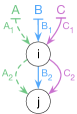
(a) Iteration graph

(b) Merge lattice for $i$

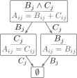
(c) Merge lattice for $j$

Figure 6. Iteration graph and optimized merge lattices for sparse matrix addition $A_{ij}=B_{ij}+C_{ij}$, where $B$ is a CSR matrix and $C$ is a COO matrix that is guaranteed to contain no empty row.

For each dimension, indexed by some index variable $v$, in the joint iteration space, its corresponding merge lattice describes what loops are needed to fully merge all input tensor dimensions that $v$ indexes into. Each point in the ordered lattice encodes a set of input tensor dimensions indexed by $v$ that may contain nonzeros and that need to be simultaneously merged in one loop. Each lattice point also encodes a sub-expression to be computed in the corresponding loop. Every path from the top lattice point to the bottom lattice point represents a sequence of loops that might have to be executed at runtime in order to fully merge the inputs. Figures 6(b) and 6(c), for instance, show merge lattices for matrix addition with a CSR matrix $B$ and a COO matrix $C$ that has no empty row. To fully merge $B$ and $C$’s column dimensions, we would start by running the loop that corresponds to the top lattice point in Figure 6(c), computing $A_{ij}=B_{ij}+C_{ij}$ in each iteration. This incrementally merges the two operands until one (e.g., $B$) has been fully merged into the output. Then, to also fully merge the other operand (i.e., $C$) into the output, we would only have to run the loop that corresponds to the middle-left lattice point in Figure 6(c), which computes $A_{ij}=C_{ij}$ in each iteration in order to copy the remaining nonzeros from $C$ to the output.

4.2. Property-Based Merge Lattice Optimizations

Optimizations on merge lattices that simplify them to yield optimized code were described by Kjolstad et al. (2017). Those were, however, all hard-coded to dense and compressed level formats. We reformulate the optimizations with respect to properties and capabilities of coordinate hierarchy levels, so that they can be applied to other level types. In particular, given a merge lattice for index variable $v$, our algorithm removes any lattice point that does not merge every full tensor dimension (i.e., a dimension represented by a full coordinate hierarchy level) that $v$ indexes into. This is valid since full tensor dimensions are supersets of any sparse dimension, so once we finish iterating over and merge a full dimension we must have also visited every coordinate in the joint iteration space. Applying this optimization gives us the optimized merge lattice shown in Figure 6(b), which contains just a single lattice point even though the computed operation requires a union merge.

Our algorithm also optimizes merging of any number of full dimensions by emitting code to co-iterate over only those that do not support the locate capability, with the rest accessed via calls to locate. Depending on whether the operands are unordered, this can reduce the complexity of the co-iteration and thus the merge, assuming locate runs in constant time.

4.3. Level Iterator Conversion

As we will see in Section 4.4, efficient algorithms exist for merging coordinate hierarchy levels that are ordered and unique, as well as for intersection merges where unordered levels provide the locate capability. Level iterator conversion turns iterators over unordered and non-unique levels without the locate capability into iterators with any desired properties. The aforementioned algorithms can then be used in conjunction to merge any coordinate hierarchy levels.

In the rest of this subsection, we describe two types of iterator conversion, deduplication and reordering, that can be composed to extend support to any combination of coordinate hierarchy levels. The flowchart on the right in Figure 8 identifies, for each operand in an intersection merge, the iterator conversions that are needed to merge the operands. Our code generation algorithm emits code to perform these necessary iterator conversions on the fly at runtime.

Deduplication

Duplicate coordinates complicate merging because it results in code that repeatedly visit the same points in the iteration space. Deduplication removes duplicates from iterators over ordered and non-unique levels using a deduplication loop. Lines 5–7 in Figure 1 shows an example of a deduplication loop that scans ahead and aggregates duplicate coordinates, resulting in an iterator that enumerates unique coordinates.

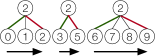
(a) Separate iterators over the duplicates’ children.

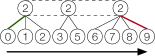
(b) Chained iterator over the duplicates’ children.

Figure 7. Iterator chaining chains the iterators over the children of duplicate coordinates (7(a)) into a single iterator over all the children (7(b)). The arrows represent iterators with start and end bounds as green and red edges.

When non-unique levels are at the bottom of coordinate hierarchies, our technique emits deduplication loops that sum the values of duplicate coordinates. Otherwise, the emitted deduplication loop combines the iterators over the duplicate coordinates’ children into a single iterator. In general, this requires a scratch array to store the child coordinates. Figure 7 shows how to avoid the scratch array by chaining together the iterators over the children. This, however, requires that the child level support position iteration and that the child and parent levels be both ordered and compact. With iterator chaining, the starting bound of the first set of children and the ending bound of the last set of children become the bounds of the chained iterator. The resulting iterator provides the same interface as a regular coordinate position iterator and can thus participate in merging without a scratch array. Figure 1 shows iterator chaining used to iterate over columns of a COO matrix.

Reordering

A precondition for code to co-iterate over levels is that coordinates are enumerated in order. Reordering uses a scratch array to store an ordered copy of an unordered level and replaces iterators over the unordered level with iterators over the ordered copy. The code generation algorithm can then emit code that merges unordered levels by co-iterating over the ordered copies.

4.4. Level Merge Code

As a result of how we defined coordinate hierarchies in Section 3, merging dimensions of tensor operands is equivalent to merging the coordinate hierarchy levels that represent those dimensions. The most efficient method for merging levels depends on the properties and supported capabilities of the merged levels. Consider, for instance, the component-wise multiplication of two vectors $x$ and $y$, which requires iterating over the intersection of coordinate hierarchy levels that encode their nonzeros. Figure 8 shows the asymptotically most efficient strategies for computing the intersection merge depending on whether the inputs are ordered or unique and whether they support the locate capability. These are the same strategies that our code generation algorithm selects.

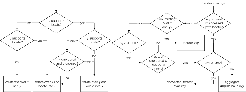
Figure 8. The most efficient strategies for computing the intersection merge of two vectors $x$ and $y$, depending on whether they support the locate capability and whether they are ordered and unique. The sparsity structure of $y$ is assumed to not be a strict subset of the sparsity structure of $x$. The flowchart on the right describes, for each operand, what iterator conversions are needed at runtime to compute the merge.

If neither input vector supports the locate capability, we can co-iterate over the coordinate hierarchy levels that represent those vectors and compute a new output component whenever we encounter nonzero components in both inputs that share the same coordinate. Lines 8–20 in Figure 1 shows another example of this method applied to merge the column dimensions of a CSR matrix and a COO matrix. This method generalizes the two-way merge algorithm used in merge sort (Knuth, 1973, Chapter 5.2.4) to compute union or intersection merges of any number of inputs. Like the two-way merge algorithm though, it depends on being able to enumerate input coordinates uniquely and in order. Nonetheless, this method can be used in conjunction with the level iterator conversions described in Section 4.3 to merge any coordinate hierarchy levels regardless of their properties, as Figure 8 demonstrates how.

If one of the input vectors, $y$, supports the locate capability (e.g., it is a dense array), we can instead just iterate over the nonzero components of $x$ and, for each component, locate the component with the same coordinate in $y$. Lines 2–9 in Figure 1 shows another example of this method applied to merge the column dimensions of a CSR matrix and a dense matrix. This alternative method reduces the merge complexity from $O(\operatorname{nnz}(x)+\operatorname{nnz}(y))$ to $O(\operatorname{nnz}(x))$ assuming locate runs in constant time. Moreover, this method does not require enumerating the coordinates of $y$ in order. We do not even need to enumerate the coordinates of $x$ in order, as long as there are no duplicates and we do not need to compute output components in order (e.g., if the output supports the insert capability). This method is thus ideal for computing intersection merges of unordered levels.

We can generalize and combine the two methods described above to compute arbitrarily complex merges involving unions and intersections of any number of tensor operands. At a high level, any merge can be computed by co-iterating over some subset of its operands and, for every enumerated coordinate, locating that same coordinate in all the remaining operands with calls to locate. Which operands need to be co-iterated can be identified recursively from the expression $expr$ that we want to compute. In particular, for each subexpression $e=e_{1}\,\,op\,\,e_{2}$ in $expr$, let $Coiter(e)$ denote the set of operand coordinate hierarchy levels that need to be co-iterated in order to compute $e$. If $op$ is an operation that requires a union merge (e.g., addition), then computing $e$ requires co-iterating over all the levels that would have to be co-iterated in order to separately compute $e_{1}$ and $e_{2}$; in other words, $Coiter(e)=Coiter(e_{1})\cup Coiter(e_{2})$. On the other hand, if $op$ is an operation that requires an intersection merge (e.g., multiplication), then the set of coordinates of nonzeros in the result $e$ must be a subset of the coordinates of nonzeros in either operand $e_{1}$ or $e_{2}$. Thus, in order to enumerate the coordinates of all nonzeros in the result, it suffices to co-iterate over all the levels merged by just one of the operands. Without loss of generality, this lets us compute $e$ without having to co-iterate over levels merged by $e_{2}$ that can instead be accessed with locate; in other words, $Coiter(e)=Coiter(e_{1})\cup(Coiter(e_{2})\,\backslash\,LocateCapable(e_{2}))$, where $LocateCapable(e_{2})$ denotes the set of levels merged by $e_{2}$ that support the locate capability.

4.5. Code Generation Algorithm

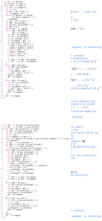
(a) Algorithm to generate tensor algebra code.

(b) Generated code, with level function calls inlined, for adding a CSR matrix to a COO matrix with no empty row, stored to a dense output matrix.

Figure 9. Algorithm for generating code that computes tensor algebra expressions on operands represented as coordinate hierarchies, and an example of code it generates. The sets coord-value-iteration-dims and coord-pos-iteration-dims exclude dimensions in noncanonical- dims. Here, canonical dimensions refer to those that do not require a scratch array (as described in Section 4.3) in order to be co-iterated.

Figure 9(a) shows our code generation algorithm, which incorporates all of the concepts we presented in the previous subsections. Each part of the algorithm is labeled from 1 to 11; throughout the discussion of the algorithm in the rest of this section, we identify relevant parts using these labels. The algorithm emits code that iterates over the proper intersections and unions of the input tensors by calling relevant access capability level functions. At points in the joint iteration space, the emitted code computes result values and assembles the output tensor by calling relevant assembly capability level functions. The emitted code is then specialized to compute with specific tensor formats by mechanically inlining all level function calls. This approach bounds the complexity of the code generation mechanism, since it only needs to account for a finite and fixed set of level capabilities and properties. The result is an algorithm that supports many disparate tensor formats and that does not need modification to add support for more level types and tensor formats. Figure 9(b) shows an example of code that our algorithm generates, with level function calls inlined.

Our algorithm takes as input a tensor algebra expression and recursively calls itself on index variables in the expression, in the order given by the corresponding iteration graph. At each recursion level, it generates code for one index variable index-var in the input expression. The algorithm begins by emitting code that initializes iterators over input coordinate hierarchy levels, which entails calling their appropriate coordinate value or position iteration level functions (1). It also emits code to perform any necessary iterator conversion described in Section 4.3 (1, 2).

The algorithm additionally constructs a merge lattice at every recursion level for the corresponding index variable in the input tensor algebra expression. This is done by applying the merge lattice construction algorithm proposed by Kjolstad et al. (2017, Section 5.1) and simplifying the resulting lattice with the first optimization described in Section 4.2. For every point $L_{p}$ in the simplified merge lattice, the algorithm then emits a loop to merge the coordinate hierarchy levels that represent input tensor dimensions that need to be merged by $L_{p}$ (4). The subset of merged levels that must be co-iterated by each loop (i.e., coiter-dims($L_{p}$)) is determined by applying the recursive algorithm described in Section 4.4 (with the sub-expression to be computed by $L_{p}$ as input) and the second optimization described in Section 4.2. Within each loop, the generated code dereferences (potentially converted) iterators over the levels that must be co-iterated (5, 7, 10), making sure to not inadvertently dereference any iterator that has exceeded its ending bound (6). The next coordinate to be visited in the joint iteration space, $iv$, is then computed (8) and used to index into the levels that can instead be accessed with the locate capability (9). At the end of each loop iteration, the generated code advances every iterator that referenced the merged coordinate $iv$ (11), so that subsequent iterations of the loop will not visit the same coordinate again.

Within each loop, the generated code must also actually compute the value of the result tensor at each coordinate as well as assemble the output indices (3). The latter entails emitting code that calls the appropriate assembly capability level functions to store result nonzeros in the output data structures. The algorithm emits specialized compute and assembly code for each merge lattice point that is dominated by $L_{p}$, which handles the case where the corresponding subset of inputs contain nonzeros at the same coordinate.

Fusing Iterators

By default, at every recursion level, the algorithm emits loops that iterate over a single coordinate hierarchy level of each input tensor. However, an optimization that improves performance when computing with formats like COO entails emitting code that simultaneously iterates over multiple coordinate hierarchy levels of one tensor. The algorithm implements this optimization by fusing iterators over branchless levels with iterators over their preceding levels. This is legal as long as the fused iterators do not need to participate in co-iteration (i.e., if the other levels to be merged can be accessed with locate). The algorithm then avoids emitting loops for levels accessed by fused iterators (4), which eliminates unnecessary branching overhead. For some computations, however, this optimization transforms the emitted kernel from a gather code that enumerates each result nonzero once to a scatter code that accumulates into the output. In such cases, the algorithm ensures the output can also be accessed with locate. Figure 1 gives an example of code this optimization generates, which iterates over two tensor dimensions with a single loop.

5. Evaluation

To evaluate our contributions, we compare code that our technique generates to five state-of-the-art sparse linear and tensor algebra libraries. We find that the sparse tensor algebra code our technique emits for many disparate formats have performance competitive with hand-implemented kernels, which shows we can get both performance and generality. We further find that our technique’s ability to support disparate tensor formats can be crucial for performance in practice.

5.1. Experimental Setup

We implemented our technique as an extension to the open-source taco tensor algebra compiler (Kjolstad et al., 2017). To evaluate it, we used taco with our extension to generate kernels that compute various sparse linear and tensor algebra operations with real-world application, including SpMV and MTTKRP. We compared the generated kernels against five other existing sparse libraries: Intel MKL (Intel, 2012), SciPy (Jones et al., 2001), MTL4 (Gottschling et al., 2007), the MATLAB Tensor Toolbox (Bader and Kolda, 2007), and TensorFlow (Abadi et al., 2016). Intel MKL is a C and Fortran math processing library that is heavily optimized for Intel processors. SciPy is a popular scientific computing library for Python. MTL4 is a C++ library that specializes linear algebra operations for fast execution using template metaprogramming. The Tensor Toolbox is a MATLAB library that implements many kernels and factorization algorithms for any-order dense and sparse tensors. TensorFlow is a machine learning library that supports some basic sparse tensor operations. We did not directly compare code generated by our technique and the approach of Kjolstad et al. (2017), since the two techniques emit identical code for formats they both support.

All experiments were run on a two-socket, 12-core/24-thread 2.4 GHz Intel Xeon E5-2695 v2 machine with 30 MB of L3 cache per socket and 128 GB of main memory, using GCC 5.4.0 and MATLAB 2016b. We ran each experiment between 10 (for longer-running benchmarks) to 100 times (for shorter-running benchmarks), with the cache cleared of input data before each run, and report average execution times. All results are for single-threaded execution.

We ran our experiments with real-world and synthetic tensors of varying sizes and structures as input, inspired by similar collections of test matrices and tensors from related works (Bell and Garland, 2008; Smith and Karypis, 2015). Table 4 describes these tensors in more detail. The real-world tensors come from applications in many disparate domains and were obtained from the SuiteSparse Matrix Collection (Davis and Hu, 2011) and the FROSTT Tensor Collection (Smith et al., 2017b). We stored tensor coordinates as integers and component values as double-precision floats, except for the Tensor Toolbox’s TTM and INNERPROD kernels. Those two kernels do not support integer coordinates, so we evaluated them with double-precision floating-point coordinates.

Table 4. Summary of matrices and tensors used in experiments.

Tensor	Domain	Dimensions	Nonzeros	Density	Diagonals
pdb1HYS	Protein data base	36K $\times$ 36K	$4,344,765$	$3\text{\times}{10}^{-3}$	$25,577$
jnlbrng1	Optimization	40K $\times$ 40K	$199,200$	$1\text{\times}{10}^{-4}$	$5$
obstclae	Optimization	40K $\times$ 40K	$197,608$	$1\text{\times}{10}^{-4}$	$5$
chem	Chemical master equation	40K $\times$ 40K	$201,201$	$1\text{\times}{10}^{-4}$	$5$
rma10	3D CFD	46K $\times$ 46K	$2,329,092$	$1\text{\times}{10}^{-3}$	$17,367$
dixmaanl	Optimization	60K $\times$ 60K	$299,998$	$8\text{\times}{10}^{-5}$	$7$
cant	FEM/Cantilever	62K $\times$ 62K	$4,007,383$	$1\text{\times}{10}^{-3}$	$99$
consph	FEM/Spheres	83K $\times$ 83K	$6,010,480$	$9\text{\times}{10}^{-4}$	$13,497$
denormal	Counter-example problem	89K $\times$ 89K	$1,156,224$	$1\text{\times}{10}^{-4}$	$13$
Baumann	Chemical master equation	112K $\times$ 112K	$748,331$	$6\text{\times}{10}^{-5}$	$7$
cop20k_A	FEM/Accelerator	121K $\times$ 121K	$2,624,331$	$2\text{\times}{10}^{-4}$	$221,205$
shipsec1	FEM	141K $\times$ 141K	$3,568,176$	$2\text{\times}{10}^{-4}$	$10,475$
scircuit	Circuit	171K $\times$ 171K	$958,936$	$3\text{\times}{10}^{-5}$	$159,419$
mac_econ	Economics	207K $\times$ 207K	$1,273,389$	$9\text{\times}{10}^{-5}$	$511$
pwtk	Wind tunnel	218K $\times$ 218K	$11,524,432$	$2\text{\times}{10}^{-4}$	$19,929$
Lin	Structural problem	256K $\times$ 256K	$1,766,400$	$3\text{\times}{10}^{-5}$	$7$
synth1	Synthetic matrix	500K $\times$ 500K	$1,999,996$	$8\text{\times}{10}^{-6}$	$4$
synth2	Synthetic matrix	1M $\times$ 1M	$1,999,999$	$2\text{\times}{10}^{-6}$	$2$
ecology1	Animal movement	1M $\times$ 1M	$4,996,000$	$5\text{\times}{10}^{-6}$	$5$
webbase	Web connectivity	1M $\times$ 1M	$3,105,536$	$3\text{\times}{10}^{-6}$	$564,259$
atmosmodd	Atmospheric model	1.3M $\times$ 1.3M	$8,814,880$	$5\text{\times}{10}^{-6}$	$7$
Facebook	Social media	1.6K $\times$ 64K $\times$ 64K	$737,934$	$1\text{\times}{10}^{-7}$
NELL-2	Machine learning	12K $\times$ 9.2K $\times$ 29K	$76,879,419$	$2\text{\times}{10}^{-5}$
NELL-1	Machine learning	2.9M $\times$ 2.1M $\times$ 25M	$143,599,552$	$9\text{\times}{10}^{-13}$

5.2. Sparse Matrix Computations

Our technique generates efficient tensor algebra kernels that are specialized to the layouts and attributes (e.g., sortedness) of the tensor operands. In this section, we compare the performance of taco-generated kernels that compute operations on COO, CSR, DIA, and ELL matrices with equivalent implementations in MKL, SciPy, MTL4, and TensorFlow.

Figure 10 shows results for sparse matrix-vector multiplication (SpMV), an important operation in many iterative methods for solving large-scale linear systems from scientific and engineering applications (Bell and Garland, 2008). Our technique is the only one that supports all the formats we survey; MTL4 does not support DIA, neither MKL nor SciPy supports ELL, and TensorFlow only supports COO. MKL and SciPy also only support the struct of arrays (SoA) variant of the COO format, which is the variant shown in Figure 2. TensorFlow, on the other hand, only supports array of structs (AoS) COO, which uses a single crd array to store coordinates for each individual tensor component contiguously in memory. By contrast, our technique supports both variants; supporting AoS COO only requires defining variants of the compressed and singleton level formats with slightly modified definitions of pos_access but the same abstract interface.

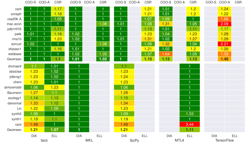
Figure 10. Normalized execution time of SpMV ($y=Ax$) with matrix $A$ stored in various formats, using taco (with our extension) and other existing libraries. Results are normalized to the fastest library for each matrix and format, and the geometric means of the results are shown in bold. Unlabeled cells in gray indicate a library does not support that format; taco is the only library that supports SpMV for all the formats we evaluate. COO-S and COO-A denote the struct-of-arrays and array-of-structs variants of COO respectively.

Figures 11 and 12 show results for sparse matrix-dense matrix multiplication (SpDM), another important operation in many data analytics and machine learning applications (Koanantakool et al., 2016), and matrix addition with sparse COO matrices. Figure 13 shows results for CSR matrix addition. Our technique is again the only one that supports all operations. SciPy does not support COO SpDM, while MTL4 only supports SpDM with sorted COO matrices. Furthermore, only TensorFlow and taco support computing COO matrix addition with a COO output, and TensorFlow does not support CSR matrix addition. These omissions highlight the advantage of a compiler approach such as ours that does not require every operation to be manually implemented.

Overall, the results show that our technique generates code that has performance competitive with existing libraries. For SpDM and sparse matrix addition, taco-emitted code consistently has performance equal to or better than other libraries. For SpMV, taco-emitted code outperforms TensorFlow, perform similar to SciPy and MTL4, and is competitive with MKL on the whole. Even for DIA, taco is only about 21% slower than MKL on average. These results are explained below.

5.2.1. COO Kernels

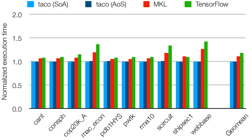
Figure 11. Normalized execution time of COO SpDM ($A=BC$, where $B$ is in COO and $A$ and $C$ are dense matrices) with taco and other libraries that support the operation, relative to taco for each matrix.

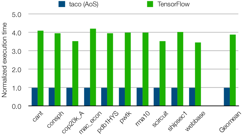
Figure 12. Normalized execution time of COO matrix addition ($A=B+C$, where all matrices are stored in the AoS COO format) with taco and TensorFlow, relative to taco for each matrix.

The code that our technique generates to compute COO SpMV implements the same algorithm as SciPy and MKL, and they therefore have the same performance. MTL4 also implements this algorithm, but stores the result of the computation in a temporary that is subsequently copied to the output. This incurs additional cache misses for matrices with larger dimensions, such as webbase. TensorFlow, on the other hand, does not implement a COO SpMV kernel and the operation must be cast as an SpDM with a single-column matrix. It therefore incurs overhead because every input vector access requires a loop over its trivial column dimension.

The COO matrix addition code that our technique emits is specialized to the order of the tensor operands. By contrast, TensorFlow has loops that iterate over the coordinates of each component. These loops let TensorFlow support tensors of any order but again introduces unnecessary overhead. TensorFlow’s sparse addition kernel is also hard-coded to compute with 64-bit coordinates, whereas taco can emit code with narrower-width coordinates, which reduces memory traffic.

5.2.2. CSR Kernels

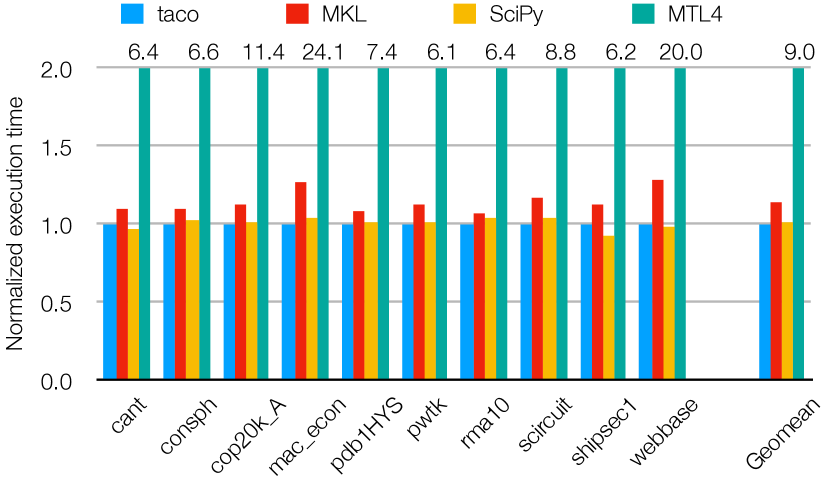
Figure 13. Normalized execution time of CSR matrix addition, relative to taco for each matrix.

Code that our technique generates for CSR SpMV iterates over the rows of the input matrix and, for each row, computes its dot product with the input vector. SciPy and MTL4 implement the same algorithm and thus have similar performance as taco, while MKL vectorizes the dot product. This, however, requires vectorizing the input vector gathers, which most SIMD architectures cannot handle very efficiently. Thus, while this optimization is beneficial with many of our test matrices (e.g., rma10), it is not always so (e.g., mac_econ).

The generated code for CSR matrix addition also uses the same algorithm as SciPy and MKL and thus has similar performance. The emitted code exploits the sortedness of the input matrices to enumerate result nonzeros in order. This lets it cheaply assemble the output crd array with appends. By contrast, MTL4 assigns one operand to a sparse temporary and then increments it by the other operand. This latter step can require significant data shuffling to keep coordinates stored in order within the sparse temporary. Finally, converting the temporary back to CSR incurs yet more overhead, leading to MTL4’s poor performance.

5.2.3. DIA and ELL SpMV

The code that our technique generates for DIA SpMV iterates over each matrix diagonal and, for each diagonal, accumulates the component-wise product of the diagonal and the input vector into the result. SciPy implements the same algorithm that taco emits and has the same performance. MKL, by contrast, tiles the computation to maximize cache utilization and thus outperform both taco and SciPy, particularly for large matrices with many diagonals. Future work includes generalizing our technique to support iteration space tiling.

Similarly, our technique generates code for ELL SpMV that iterates over matrix components in the order they are laid out in memory. MTL4, on the other hand, iterates over components row by row to maximize the cache hits for vector accesses. This lets MTL4 marginally outperform taco for matrices with few nonzeros per row. When the number of nonzeros per row is large, however, this approach reduces the cache hit rate for the matrix accesses, since components adjacent in memory are not accessed consecutively. The cost can be significant, as the results for the cant matrix show.

5.3. Sparse Tensor Computations

We also compare the performance of the following higher-order tensor kernels generated with our technique to hand-implemented kernels in the Tensor Toolbox (TTB) and TensorFlow (TF):

TTV:

$A_{ij}=\sum_{k}B_{ijk}c_{k}$

TTM:

$A_{ijk}=\sum_{l}B_{ijl}C_{kl}$

PLUS:

$A_{ijk}=B_{ijk}+C_{ijk}$

MTTKRP:

$A_{ij}=\sum_{k,l}B_{ikl}C_{kj}D_{lj}$

INNERPROD:

$\alpha=\sum_{i,j,k}B_{ijk}C_{ijk}$

where 3rd-order tensors and the outputs of TTV, TTM, and PLUS are stored in the COO format with ordered coordinates, while all other operands are dense. All these operations have real-world applications. The TTM and MTTKRP operations, for example, are building blocks of widely used algorithms for computing Tucker and CP decompositions (Liu et al., 2017; Smith et al., 2015). These same operations were also evaluated in Kjolstad et al. (2017, Section 8.4), though that work measured the performance of taco-generated code that compute with the more efficient CSF format.

Table 5. Execution times of sparse COO tensor algebra kernels in milliseconds. Figures in parentheses are slowdowns relative to taco. A missing entry means a library does not support an operation, while OOM means the kernel runs out of memory. NELL-2 and NELL-1 are too large for TensorFlow’s protocol buffers.

	Facebook			NELL-2		NELL-1
	taco	TTB	TF	taco	TTB	taco	TTB
TTV	13	55 (4.1$\times$)		337	4797 (14.3$\times$)	2253	11239 (5.0$\times$)
TTM	444	18063 (40.7$\times$)		5350	48806 (9.1$\times$)	56478	OOM
PLUS	37	539 (14.6$\times$)	60 (1.6$\times$)	3085	73380 (23.8$\times$)	6289	123387 (19.6$\times$)
MTTKRP	44	364 (8.4$\times$)		3819	43102 (11.3$\times$)	21042	110502 (5.3$\times$)
INNERPROD	12	670 (57.1$\times$)		416	82748 (199.0$\times$)	985	148592 (150.9$\times$)

Table 5 shows the results of this experiment, with Intel MKL, SciPy, and MTL4 omitted as they do not support sparse higher-order tensor algebra. The Tensor Toolbox and TensorFlow are on opposite sides of the trade-off space for hand-written sparse libraries. The Tensor Toolbox supports all the operations in our benchmark but has poor performance, while TensorFlow supports only one operation but is more efficient than the Tensor Toolbox. Our technique, by contrast, emits efficient code for all five operations, showing generality and performance are not mutually exclusive.

As with sparse matrix addition, the code that taco with our extension generates for adding 3rd-order COO tensors has better performance than TensorFlow’s generic sparse tensor addition kernel. Furthermore, taco generates code that significantly outperforms the Tensor Toolbox kernels, often by more than an order of magnitude. This is because the Tensor Toolbox relies on MATLAB functionalities that cannot directly operate on tensor indices or exploit tensor properties to optimize the computation. To add two sparse tensors, for instance, the Tensor Toolbox computes the set of output nonzero coordinates by calling a MATLAB built-in function that computes the union of the sets of input nonzero coordinates. MATLAB’s implementation of set union, however, cannot exploit the fact that the inputs are already individually sorted and must sort the concatenation of the two input indices. By contrast, taco emits code that directly iterates over and merges the two input indices without first re-sorting them, reducing the asymptotic complexity of the computation. Additionally, taco emits code that directly assembles sparse output indices, whereas for computations such as TTM the Tensor Toolbox stores the results in intermediate dense structures.

5.4. Benefits of Supporting Disparate Formats

Table 6. Support for various sparse tensor formats by taco with our extension (this work) and without ((Kjolstad et al., 2017)) as well as by other existing sparse linear and tensor algebra libraries. (✓) identifies tensor formats that our technique can support by defining additional level formats.

Tensor Type	Format	taco		MKL	SciPy	MTL4	TTB	TF
		This Work	(Kjolstad et al., 2017)
Vector	Sparse vector	✓	✓	✓	✓	✓	✓	✓
	Hash map	✓			✓
Matrix	COO	✓		✓	✓	✓	✓	✓
	CSR	✓	✓	✓	✓	✓	✓
	DCSR	✓	✓
	ELL	✓				✓
	DIA	✓		✓	✓
	BCSR	✓	✓	✓	✓	✓
	CSB	✓
	DOK				✓
	LIL				✓
	Skyline	(✓)		✓
	Banded	(✓)				✓
3rd-Order Tensor	COO	✓					✓	✓
	CSF	✓	✓
	Mode-generic	✓

Table 6 more comprehensively shows, for a wide variety of sparse tensor formats, which formats are supported by our technique, the approach of Kjolstad et al. (2017), and the other existing sparse linear and tensor algebra libraries we evaluate. In addition to the formats described in Section 2, we also consider all the other formats for storing unfactorized, non-symmetric sparse tensors that are supported by at least one existing library. This includes DOK (The SciPy community, 2018a), which uses a hash map indexed by both row and column coordinates to encode both dimensions of a matrix in a shared data structure, and LIL (The SciPy community, 2018b), which uses linked lists to store the nonzeros of each matrix row. Additionally, the skyline format (A. Remington, 1996) is a format designed for storing variably-banded triangular matrices, while the (sparse) banded matrix format is similar to DIA but instead stores components in each row contiguously. Our technique, on the whole, supports a much larger and more diverse set of sparse tensor formats than other existing libraries and the approach of Kjolstad et al. (2017). Furthermore, our technique can be extended to support the skyline and banded matrix formats by defining additional level formats that use their data structures. Fully supporting DOK and LIL, however, requires extensions to the coordinate hierarchy abstraction, which we believe is interesting future work. To be able to emit code that randomly access DOK matrices, the locate capability would need to effectively permit traversing multiple coordinate hierarchy levels with a single call to locate. Additionally, to support LIL would require our abstraction to support storing component values non-contiguously in memory.

Our technique’s support for more disparate formats can enable it to outperform the approach of Kjolstad et al. (2017) in practical use, depending on characteristics of the computation and data. The COO format, for instance, is the intuitive way to represent sparse tensors and is used by many file formats to encode sparse tensors. Thus, it is a natural format for importing and exporting sparse tensors into and out of an application. As the blue bars in Figure 14 show, computing matrix-vector products directly on COO matrices can take up to twice as much time as with CSR matrices due to higher memory traffic. If a matrix is imported into the application in the COO format though, then it must be converted to a CSR matrix before the more efficient CSR SpMV kernel can be used. This preprocessing step incurs significant overhead that, as the red bars in Figure 14 show, exceeds the cost of computing on the original COO matrix. For non-iterative applications that cannot amortize this conversion overhead, our technique offers better end-to-end performance by enabling SpMV to be computed directly on the COO input matrix, thereby eliminating the overhead.

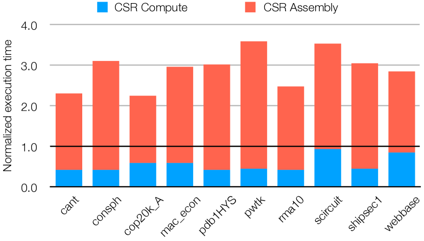
Figure 14. Normalized execution time of CSR SpMV relative to COO SpMV, taking into account the cost of assembling CSR indices for the input matrices. These results show that computing with CSR is faster than with COO (black line) only if the cost of assembling CSR indices can be amortized over multiple iterations.

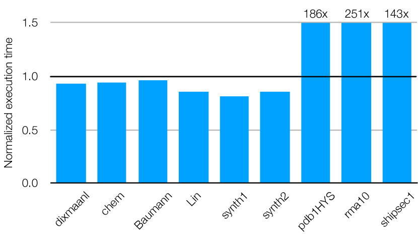
Figure 15. Normalized execution time of taco’s DIA SpMV kernel relative to taco’s CSR SpMV kernel. Storing the input matrix in the DIA format can accelerate SpMV if all the nonzeros in the matrix are confined to a few densely-filled diagonals, but can drastically degrade performance if that is not the case.

Which format is most performant also depends on the tensor’s sparsity structure. To show this, we compare the performance of SpMV computed on CSR and DIA matrices using taco-generated kernels. For matrices like Lin and synth1 whose nonzeros are all in a few densely-filled diagonals, storing them in DIA exposes opportunities for vectorization. As Figure 15 shows, our technique can exploit them to improve SpMV performance by up to 22% relative to the approach of Kjolstad et al. (2017), which only supports CSR SpMV. However, DIA SpMV performs significantly worse for matrices like rma10 whose nonzeros are spread amongst many sparsely-filled diagonals, since it has to unnecessarily compute with all the zeros in the nonempty diagonals.

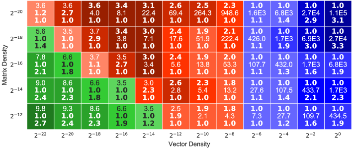
Figure 16. Normalized execution time of taco’s CSR SpMV with inputs of varying density and input vectors stored in different formats, relative to the most performant format for each configuration. Each cell shows results for dense arrays (top), sparse vectors (middle), and hash maps (bottom). Cells are highlighted based on which vector format is most performant (blue for dense arrays, green for sparse vectors, red for hash maps).

We further compare the performance of CSR SpMV with input vectors stored as dense arrays, sparse vectors, and hash maps, for operands of varying density. Figure 16 shows the results. When the input vector contains mostly nonzeros, dense arrays are suitable for SpMV as they provide efficient random access without needing to explicitly store coordinates of nonzeros. Conversely, when the input vector contains mostly zeros and the matrix is much denser, sparse vectors offer better performance for SpMV as it can be computed without accessing all matrix nonzeros. However, when the input vector is large and sparse but still denser than the matrix, computing SpMV with hash map vectors reduces the number of accesses that go out of cache. At the same time, the hash map format’s random access capability makes it possible to compute SpMV without accessing the full input vector. This enables the our technique, with its support for hash maps, to outperform the approach of Kjolstad et al. (2017), which only supports the dense array and sparse vector formats.

6. Related Works

Related work in this area can be categorized into explorations of sparse tensor formats and prior work on abstractions for sparse tensor storage and code generation for sparse tensor computations.

6.1. Sparse Tensor Formats

There is a large body of work on sparse matrix and higher-order tensor formats. Sparse matrix data structures were first introduced by Tinney and Walker (1967), who appear to have implemented the CSR data structure. McNamee (1971) described an early library that supports computations on sparse matrices stored in a compressed variant of CSR. The analogous CSC format is also commonly used partly because it is convenient for direct solves (Davis, 2006). Many other formats for storing sparse matrices and higher-order tensors have since been proposed; Section 2 describes them in detail. This work shows that all these tensor formats can be represented within the same framework with just six composable level formats that share a common interface.

Other proposed sparse tensor formats include BICRS (Yzelman and Bisseling, 2012), which extends the CSR format to efficiently store nonzeros of a sparse matrix in Hilbert order. For efficiently computing SpMV on GPUs, Monakov et al. (2010) proposed sliced ELLPACK, which generalizes ELL by partitioning the matrix into strips of a fixed number of adjacent rows, with each strip possibly storing a different number of nonzeros per row so as to minimize the number of stored zeros. Liu et al. (2017) also proposed F-COO, which extends COO for enabling efficient computation of sparse higher-order tensor kernels on GPUs. Bell and Garland (2008) described the HYB format, which stores most components of a matrix in an ELL submatrix and the remaining components in another COO submatrix. The HYB format is useful for computing SpMV on vector architectures with matrices that contain similar numbers of nonzeros in most rows but have a few rows that contain many more nonzeros. The Cocktail Format in clSpMV (Su and Keutzer, 2012), generalizes HYB to support any number of submatrices stored in one of nine fixed sparse matrix formats.

6.2. Tensor Storage Abstractions and Code Generation

Researchers have also explored approaches to describing sparse vector and matrix storage for sparse linear algebra. Thibault et al. (1994) proposed a technique that describes regular geometric partitions in arrays and automatically generates corresponding indexing functions. The technique compresses matrices with regular structure, but does not generalize to unstructured matrices.

In the context of compilers for sparse linear and tensor algebra, Kjolstad et al. (2017) proposed a formulation for tensor formats that designates each dimension as either dense or sparse, which are stored using the same data structures as dense and compressed level types in our abstraction. However, their formulation can only describe formats that are composed strictly of those two specific types of data structures, which precludes their technique from generating tensor algebra kernels that compute on many other common formats like COO and DIA. The Bernoulli project (Kotlyar et al., 1997; Stodghill, 1997; Kotlyar, 1999), which adopted a relational database approach to sparse linear algebra compilation, proposed a black-box protocol with access paths that describe how matrices map to physical storage. The black-box protocol is similar to our level format interface, but they only address linear algebra and only computations involving multiplications and not additions. The black-box protocol also does not support on-the-fly assembly of sparse indices, which is often essential for applications with sparse high-order outputs. SIPR (Pugh and Shpeisman, 1999), a framework that transforms dense linear algebra code to sparse code, represents sparse vectors and matrices with hard-coded element stores that provide enumerators and accessors that are analogous to level capabilities. The framework provides just two types of element store and cannot be readily extended to support new types of element store for representing other formats. Arnold et al. (2010; 2011) proposed LL, a verifiable functional language for sparse matrix programs in which a sparse matrix format is defined as some nesting of lists and pairs that encode components of a dense matrix. How an LL format should be interpreted is described as part of the computation in LL, so the same computation with different matrix formats can require completely different definitions.

Bik and Wijshoff (1993; 1994) developed an early compiler that transforms dense linear algebra code to equivalent sparse code by moving nonzero guards into sparse data structures. More recently, Venkat et al. (2015) proposed a technique for generating inspector/executor code that may, at runtime, transform input matrices from one format to another. Both techniques support a fixed set of standard sparse matrix formats and only generate code that work with matrices stored in those formats. Finally, Rong et al. (2016) proposed a technique that discovers and exploits invariant properties of matrices in a sparse linear algebra program to optimize the program as a whole.

Much work has also been done on compilers (Spampinato and Püschel, 2014; Nelson et al., 2015) and loop transformation techniques (Wolfe, 1982; Wolf and Lam, 1991; McKinley et al., 1996) for dense linear algebra. An early effort for dense higher-order tensor algebra was the Tensor Contraction Engine (Auer et al., 2006). libtensor (Epifanovsky et al., 2013), CTF (Solomonik et al., 2014), and GETT (Springer and Bientinesi, 2016) are examples of systems and techniques that transform tensor contractions into dense matrix multiplications by transposing tensor operands. TBLIS (Matthews, 2017) and InTensLi (Li et al., 2015) avoid explicit transpositions by computing tensor contractions in-place. All of these systems and techniques deal exclusively with tensors stored as dense arrays.

7. Conclusion and Future Work

We have described and implemented a new technique for generating tensor algebra kernels that efficiently compute on tensors stored in disparate formats. Our technique’s modularity enables it to support many formats and to be extended to new formats without having to modify the code generator. This makes our technique practical for disparate domains that need to efficiently perform different types of computations with dissimilar data. Large-scale applications that need performance may also have to use multiple formats that are each optimized for a different subcomputation. A technique like ours that shapes computation to data makes it possible to work with different formats without incurring excessive data translation costs, thus optimizing whole-program performance.

Future work includes extending our technique to support even more disparate tensor formats, including DOK and LIL as well as custom formats designed to take advantage of power-law structures in social graphs for graph analytics or specialized hardware accelerator capabilities for deep learning architectures (Chen et al., 2017). Additional examples include formats that exploit structural and value symmetries, which are common in many scientific and engineering domains, to reduce memory footprint. Another direction of future work is to extend the code generation algorithm to emit shared-memory parallel code and perform further optimizations like iteration space tiling, as well as specifically target accelerators (e.g., GPUs) and distributed memory systems. Our modular approach enables these lines of research to be pursued independently.

- (1)
- A. Remington (1996) Karin A. Remington. 1996. NIST Sparse BLAS User’s Guide. (08 1996).
- Abadi et al. (2016) Martín Abadi, Paul Barham, Jianmin Chen, Zhifeng Chen, Andy Davis, Jeffrey Dean, Matthieu Devin, Sanjay Ghemawat, Geoffrey Irving, Michael Isard, Manjunath Kudlur, Josh Levenberg, Rajat Monga, Sherry Moore, Derek G. Murray, Benoit Steiner, Paul Tucker, Vijay Vasudevan, Pete Warden, Martin Wicke, Yuan Yu, and Xiaoqiang Zheng. 2016. TensorFlow: A System for Large-scale Machine Learning. In Proceedings of the 12th USENIX Conference on Operating Systems Design and Implementation (OSDI’16). USENIX Association, Berkeley, CA, USA, 265–283. http://dl.acm.org/citation.cfm?id=3026877.3026899
- Anandkumar et al. (2014) Animashree Anandkumar, Rong Ge, Daniel Hsu, Sham M. Kakade, and Matus Telgarsky. 2014. Tensor Decompositions for Learning Latent Variable Models. J. Mach. Learn. Res. 15, Article 1 (Jan. 2014), 60 pages.
- Arnold (2011) Gilad Arnold. 2011. Data-Parallel Language for Correct and Efficient Sparse Matrix Codes. Ph.D. Dissertation. University of California, Berkeley.
- Arnold et al. (2010) Gilad Arnold, Johannes Hölzl, Ali Sinan Köksal, Rastislav Bodík, and Mooly Sagiv. 2010. Specifying and Verifying Sparse Matrix Codes. In Proceedings of the 15th ACM SIGPLAN International Conference on Functional Programming (ICFP ’10). ACM, New York, NY, USA, 249–260. https://doi.org/10.1145/1863543.1863581
- Auer et al. (2006) Alexander A. Auer, Gerald Baumgartner, David E. Bernholdt, Alina Bibireata, Venkatesh Choppella, Daniel Cociorva, Xiaoyang Gao, Robert Harrison, Sriram Krishnamoorthy, Sandhya Krishnan, Chi-Chung Lam, Qingda Lu, Marcel Nooijen, Russell Pitzer, J. Ramanujam, P. Sadayappan, and Alexander Sibiryakov. 2006. Automatic code generation for many-body electronic structure methods: the tensor contraction engine. Molecular Physics 104, 2 (2006), 211–228.
- Bader and Kolda (2007) Brett W Bader and Tamara G Kolda. 2007. Efficient MATLAB computations with sparse and factored tensors. SIAM Journal on Scientific Computing 30, 1 (2007), 205–231.
- Baskaran et al. (2012) M. Baskaran, B. Meister, N. Vasilache, and R. Lethin. 2012. Efficient and scalable computations with sparse tensors. In 2012 IEEE Conference on High Performance Extreme Computing. 1–6. https://doi.org/10.1109/HPEC.2012.6408676
- Bell and Garland (2008) Nathan Bell and Michael Garland. 2008. Efficient Sparse Matrix-Vector Multiplication on CUDA. NVIDIA Technical Report NVR-2008-004. NVIDIA Corporation.
- Bik and Wijshoff (1993) Aart JC Bik and Harry AG Wijshoff. 1993. Compilation techniques for sparse matrix computations. In Proceedings of the 7th international conference on Supercomputing. ACM, 416–424.
- Bik and Wijshoff (1994) Aart JC Bik and Harry AG Wijshoff. 1994. On automatic data structure selection and code generation for sparse computations. In Languages and Compilers for Parallel Computing. Springer, 57–75.
- Buluç et al. (2009) Aydin Buluç, Jeremy T Fineman, Matteo Frigo, John R Gilbert, and Charles E Leiserson. 2009. Parallel sparse matrix-vector and matrix-transpose-vector multiplication using compressed sparse blocks. In Proceedings of the twenty-first annual symposium on Parallelism in algorithms and architectures. ACM, 233–244.
- Buluç and Gilbert (2008) Aydin Buluç and John R. Gilbert. 2008. On the representation and multiplication of hypersparse matrices. In IEEE International Symposium on Parallel and Distributed Processing, (IPDPS). 1–11.
- Chen et al. (2017) Y. H. Chen, T. Krishna, J. S. Emer, and V. Sze. 2017. Eyeriss: An Energy-Efficient Reconfigurable Accelerator for Deep Convolutional Neural Networks. IEEE Journal of Solid-State Circuits 52, 1 (Jan 2017), 127–138. https://doi.org/10.1109/JSSC.2016.2616357
- Davis (2006) Timothy A Davis. 2006. Direct methods for sparse linear systems. SIAM.
- Davis and Hu (2011) Timothy A. Davis and Yifan Hu. 2011. The University of Florida Sparse Matrix Collection. ACM Trans. Math. Softw. 38, 1, Article 1 (Dec. 2011).
- D’Azevedo et al. (2005) Eduardo F. D’Azevedo, Mark R. Fahey, and Richard T. Mills. 2005. Vectorized Sparse Matrix Multiply for Compressed Row Storage Format. In Proceedings of the 5th International Conference on Computational Science - Volume Part I (ICCS’05). Springer-Verlag, Berlin, Heidelberg, 99–106. https://doi.org/10.1007/11428831_13
- Epifanovsky et al. (2013) Evgeny Epifanovsky, Michael Wormit, Tomasz Kuś, Arie Landau, Dmitry Zuev, Kirill Khistyaev, Prashant Manohar, Ilya Kaliman, Andreas Dreuw, and Anna I Krylov. 2013. New implementation of high-level correlated methods using a general block tensor library for high-performance electronic structure calculations. Journal of computational chemistry 34, 26 (2013), 2293–2309.
- Feynman et al. (1963) Richard Feynman, Robert B. Leighton, and Matthew L. Sands. 1963. The Feynman Lectures on Physics. Vol. 3. Addison-Wesley.
- Gottschling et al. (2007) Peter Gottschling, David S. Wise, and Michael D. Adams. 2007. Representation-transparent Matrix Algorithms with Scalable Performance. In Proceedings of the 21st Annual International Conference on Supercomputing (ICS ’07). ACM, New York, NY, USA, 116–125. https://doi.org/10.1145/1274971.1274989
- Im and Yelick (1998) Eun-jin Im and Katherine Yelick. 1998. Model-Based Memory Hierarchy Optimizations for Sparse Matrices. In In Workshop on Profile and Feedback-Directed Compilation.
- Intel (2012) Intel. 2012. Intel math kernel library reference manual. Technical Report. 630813-051US, 2012. http://software.intel.com/sites/products/documentation/hpc/mkl/mklman/mklman.pdf.
- Jones et al. (2001) Eric Jones, Travis Oliphant, Pearu Peterson, et al. 2001. SciPy: Open source scientific tools for Python. http://www.scipy.org/ [Online; accessed ¡today¿].
- Kincaid et al. (1989) David R. Kincaid, Thomas C. Oppe, and David M. Young. 1989. ITPACKV 2D User’s Guide.
- Kjolstad et al. (2017) Fredrik Kjolstad, Shoaib Kamil, Stephen Chou, David Lugato, and Saman Amarasinghe. 2017. The Tensor Algebra Compiler. Proc. ACM Program. Lang. 1, OOPSLA, Article 77 (Oct. 2017), 29 pages. https://doi.org/10.1145/3133901
- Knuth (1973) Donald Ervin Knuth. 1973. The art of computer programming: sorting and searching. Vol. 3. Pearson Education.
- Koanantakool et al. (2016) P. Koanantakool, A. Azad, A. Buluç, D. Morozov, S. Y. Oh, L. Oliker, and K. Yelick. 2016. Communication-Avoiding Parallel Sparse-Dense Matrix-Matrix Multiplication. In 2016 IEEE International Parallel and Distributed Processing Symposium (IPDPS). 842–853. https://doi.org/10.1109/IPDPS.2016.117
- Kolecki (2002) Joseph C Kolecki. 2002. An Introduction to Tensors for Students of Physics and Engineering. Unixenguaedu 7, September (2002), 29.
- Kotlyar (1999) Vladimir Kotlyar. 1999. Relational Algebraic Techniques for the Synthesis of Sparse Matrix Programs. Ph.D. Dissertation. Cornell.
- Kotlyar et al. (1997) Vladimir Kotlyar, Keshav Pingali, and Paul Stodghill. 1997. A relational approach to the compilation of sparse matrix programs. In Euro-Par’97 Parallel Processing. Springer, 318–327.
- Li et al. (2015) Jiajia Li, Casey Battaglino, Ioakeim Perros, Jimeng Sun, and Richard Vuduc. 2015. An input-adaptive and in-place approach to dense tensor-times-matrix multiply. In Proceedings of the International Conference for High Performance Computing, Networking, Storage and Analysis. ACM, 76.
- Liu et al. (2017) B. Liu, C. Wen, A. D. Sarwate, and M. M. Dehnavi. 2017. A Unified Optimization Approach for Sparse Tensor Operations on GPUs. In 2017 IEEE International Conference on Cluster Computing (CLUSTER). 47–57. https://doi.org/10.1109/CLUSTER.2017.75
- Matthews (2017) Devin Matthews. 2017. High-Performance Tensor Contraction without Transposition. Technical Report.
- McKinley et al. (1996) Kathryn S McKinley, Steve Carr, and Chau-Wen Tseng. 1996. Improving data locality with loop transformations. ACM Transactions on Programming Languages and Systems (TOPLAS) 18, 4 (1996), 424–453.
- McNamee (1971) John Michael McNamee. 1971. Algorithm 408: a sparse matrix package (part I)[F4]. Commun. ACM 14, 4 (1971), 265–273.
- Monakov et al. (2010) Alexander Monakov, Anton Lokhmotov, and Arutyun Avetisyan. 2010. Automatically Tuning Sparse Matrix-Vector Multiplication for GPU Architectures. In High Performance Embedded Architectures and Compilers, Yale N. Patt, Pierfrancesco Foglia, Evelyn Duesterwald, Paolo Faraboschi, and Xavier Martorell (Eds.). Springer Berlin Heidelberg, Berlin, Heidelberg, 111–125.
- National Institute of Standards and Technology (2013) National Institute of Standards and Technology. 2013. Matrix Market: File Formats. http://math.nist.gov/MatrixMarket/formats.html
- Nelson et al. (2015) Thomas Nelson, Geoffrey Belter, Jeremy G. Siek, Elizabeth Jessup, and Boyana Norris. 2015. Reliable Generation of High-Performance Matrix Algebra. ACM Trans. Math. Softw. 41, 3, Article 18 (June 2015), 27 pages.
- Pugh and Shpeisman (1999) William Pugh and Tatiana Shpeisman. 1999. SIPR: A new framework for generating efficient code for sparse matrix computations. In Languages and Compilers for Parallel Computing. Springer, 213–229.
- Rong et al. (2016) Hongbo Rong, Jongsoo Park, Lingxiang Xiang, Todd A. Anderson, and Mikhail Smelyanskiy. 2016. Sparso: Context-driven Optimizations of Sparse Linear Algebra. In Proceedings of the 2016 International Conference on Parallel Architectures and Compilation. ACM, 247–259.
- Saad (2003) Yousef Saad. 2003. Iterative methods for sparse linear systems. SIAM.
- Smith et al. (2017a) Shaden Smith, Jee W. Choi, Jiajia Li, Richard Vuduc, Jongsoo Park, Xing Liu, and George Karypis. 2017a. FROSTT file formats. http://frostt.io/tensors/file-formats.html
- Smith et al. (2017b) Shaden Smith, Jee W. Choi, Jiajia Li, Richard Vuduc, Jongsoo Park, Xing Liu, and George Karypis. 2017b. FROSTT: The Formidable Repository of Open Sparse Tensors and Tools. http://frostt.io/
- Smith and Karypis (2015) Shaden Smith and George Karypis. 2015. Tensor-matrix products with a compressed sparse tensor. In Proceedings of the 5th Workshop on Irregular Applications: Architectures and Algorithms. ACM, 5.
- Smith et al. (2015) Shaden Smith, Niranjay Ravindran, Nicholas Sidiropoulos, and George Karypis. 2015. SPLATT: Efficient and Parallel Sparse Tensor-Matrix Multiplication. In 2015 IEEE International Parallel and Distributed Processing Symposium (IPDPS). 61–70.
- Solomonik et al. (2014) Edgar Solomonik, Devin Matthews, Jeff R Hammond, John F Stanton, and James Demmel. 2014. A massively parallel tensor contraction framework for coupled-cluster computations. J. Parallel and Distrib. Comput. 74, 12 (2014), 3176–3190.
- Spampinato and Püschel (2014) Daniele G Spampinato and Markus Püschel. 2014. A basic linear algebra compiler. In Proceedings of Annual IEEE/ACM International Symposium on Code Generation and Optimization. ACM, 23.
- Springer and Bientinesi (2016) Paul Springer and Paolo Bientinesi. 2016. Design of a high-performance GEMM-like Tensor-Tensor Multiplication. arXiv preprint arXiv:1607.00145 (2016).
- Stodghill (1997) Paul Stodghill. 1997. A Relational Approach to the Automatic Generation of Sequential Sparse Matrix Codes. Ph.D. Dissertation. Cornell.
- Su and Keutzer (2012) Bor-Yiing Su and Kurt Keutzer. 2012. clSpMV: A Cross-Platform OpenCL SpMV Framework on GPUs. In Proceedings of the 26th ACM International Conference on Supercomputing (ICS ’12). ACM, New York, NY, USA, 353–364. https://doi.org/10.1145/2304576.2304624
- The SciPy community (2018a) The SciPy community. 2018a. scipy.sparse.dok_matrix – SciPy v1.1.0 Reference Guide. https://docs.scipy.org/doc/scipy/reference/generated/scipy.sparse.dok_matrix.html.
- The SciPy community (2018b) The SciPy community. 2018b. scipy.sparse.lil_matrix – SciPy v1.1.0 Reference Guide. https://docs.scipy.org/doc/scipy/reference/generated/scipy.sparse.lil_matrix.html.
- Thibault et al. (1994) Scott Thibault, Lenore Mullin, and Matt Insall. 1994. Generating Indexing Functions of Regularly Sparse Arrays for Array Compilers.
- Tinney and Walker (1967) William F Tinney and John W Walker. 1967. Direct solutions of sparse network equations by optimally ordered triangular factorization. Proc. IEEE 55, 11 (1967), 1801–1809.
- Venkat et al. (2015) Anand Venkat, Mary Hall, and Michelle Strout. 2015. Loop and Data Transformations for Sparse Matrix Code. In Proceedings of the 36th ACM SIGPLAN Conference on Programming Language Design and Implementation (PLDI 2015). 521–532.
- Wolf and Lam (1991) Michael E. Wolf and Monica S. Lam. 1991. A Data Locality Optimizing Algorithm. SIGPLAN Not. 26, 6 (May 1991), 30–44.
- Wolfe (1982) Michael Joseph Wolfe. 1982. Optimizing Supercompilers for Supercomputers. Ph.D. Dissertation. University of Illinois at Urbana-Champaign, Champaign, IL, USA. AAI8303027.
- Yzelman and Bisseling (2012) Albert-Jan N. Yzelman and Rob H. Bisseling. 2012. A Cache-Oblivious Sparse Matrix–Vector Multiplication Scheme Based on the Hilbert Curve. In Progress in Industrial Mathematics at ECMI 2010, Michael Günther, Andreas Bartel, Markus Brunk, Sebastian Schöps, and Michael Striebel (Eds.). Springer Berlin Heidelberg, Berlin, Heidelberg, 627–633.