Radiative Charge Transfer Between the Helium Ion and Argon

Abstract

The rate coefficient for radiative charge transfer between the helium ion and an argon atom is calculated. The rate coefficient is about $10^{-14}\;\textrm{cm}^{3}/\textrm{s}$ at 300 K in agreement with earlier experimental data.

1 Introduction

The molecular ion ${}^{36}\textrm{ArH}^{+}$ (argonium) was identified through its rotational transitions in the sub-millimeter wavelengths toward the Crab Nebula using SPIRE onboard the Herschel Space Observatory (Barlow et al., 2013), with earlier and later observations revealing ${}^{36}\textrm{ArH}^{+}$ and ${}^{38}\textrm{ArH}^{+}$ in the diffuse interstellar medium using Herschel/HIFI (Schilke et al., 2014). With the ALMA Observatory, the red-shifted spectra of $\textrm{ArH}^{+}$ was detected in an external galaxy (Müller et al., 2015). Chemical modeling indicates that the presence of $\textrm{ArH}^{+}$ may serve as a tracer of atomic gas in the very diffuse interstellar medium and as an indicator of cosmic ray ionization rates (Müller et al., 2015; Neufeld & Wolfire, 2016).

Ar created in the supernova is predominately ${}^{36}\textrm{Ar}$ and it was the isotope differences of ${}^{36}\textrm{ArH}^{+}$ absorption spectra compared to ${}^{38}\textrm{ArH}^{+}$ absorption spectra that provided the crucial clues leading to the initial identification in the Crab nebula (Barlow et al., 2013). Recently, Priestley et al. (2017) modeled $\textrm{ArH}^{+}$ formation in the filaments of the Crab nebula, considering the specific high-energy synchrotron radiation found there, in addition to the cosmic ray flux considered earlier for applications to the ISM. A detailed exploration of model parameters led Priestley et al. (2017) to the conclusion that in order to reproduce observed abundances the relevant cosmic ray ionization rate is $10^{7}$ times larger than the standard interstellar value, though sensitivity to other parameters, such as to the rate for dissociative recombination of $\textrm{ArH}^{+}$, was noted.

In models of the Crab Nebula $\textrm{Ar}^{+}$ ions are produced through cosmic ray, UV and X-ray ionizations and by the reaction of $\textrm{H}_{2}^{+}$ with Ar (Jenkins, 2013; Roueff et al., 2014). The $\textrm{ArH}^{+}$ is formed by the ion-atom interchange reaction (Barlow et al., 2013)

$$\textrm{Ar}^{+}+\textrm{H}_{2}\rightarrow\textrm{ArH}^{+}+\textrm{H}$$ (1)

and destroyed by reaction with $\textrm{H}_{2}$ (Barlow et al., 2013; Roueff et al., 2014). Sources of $\textrm{Ar}^{+}$ that enter the chemical models were detailed by Schilke et al. (2014) and Priestley et al. (2017) and include photoionization of Ar and photodissociation of $\textrm{ArH}^{+}$. As He II is present in the Crab nebula (Sankrit et al., 1998; Hester, 2008) it is fitting to investigate whether an additional source of $\textrm{Ar}^{+}$ might arise from charge transfer in Ar and $\textrm{He}^{+}$ collisions. Previous studies (Smith et al., 1970; Isler, 1974; Albat & Wirsam, 1977) indicate that the direct charge transfer process

$$\textrm{Ar}(^{1}\textrm{S})+\textrm{He}^{+}(^{2}\textrm{S})\rightarrow\textrm{Ar}^{+}(3p^{5}\;{}^{2}\textrm{P}^{\mathrm{o}})+\textrm{He}(1s^{2}\;{}^{1}\textrm{S})$$ (2)

occurs through mechanisms involving couplings to excited molecular states that are inaccessible at thermal energies and we conclude that charge transfer at thermal energies will proceed by the radiative charge transfer (RCT) mechanism

$$\textrm{Ar}+\textrm{He}^{+}\rightarrow\textrm{Ar}^{+}+\textrm{He}+h\nu,$$ (3)

where $h\nu$ is the photon energy. Experimentally, the rate coefficient for the loss of helium ions in argon gas was found by Johnsen et al. (1973) to be no more than $10^{-13}\;\textrm{cm}^{3}/\textrm{s}$ at 295 K, while Jones et al. (1979) found that the rate coefficient is greater than $2\times 10^{-14}\;\textrm{cm}^{3}/\textrm{s}$ at 300 K; both consistent with the early estimate of less than $10^{-13}\;\textrm{cm}^{3}/\textrm{s}$ at 300 K (Fehsenfeld et al., 1966). Thus, (3) is likely to be relatively slow, but we are unaware of any detailed calculations for the cross sections and rate coefficients of (3).

2 Molecular Calculations

The molecular potential energy curve (PEC) of $\textrm{HeAr}^{+}$ corresponding to the initial $\textrm{Ar}(^{1}\textrm{S})$ atom and $\textrm{He}^{+}(^{2}\textrm{S})$ ion is the $\textrm{B}\,{}^{2}\Sigma^{+}$ state, which lies 8.225 eV (Stärk & Peyerimhoff, 1986) above the $\textrm{X}\,{}^{2}\Sigma^{+}$ and the $\textrm{A}\,{}^{2}\Pi$ electronic states which correlate to the final products $\textrm{Ar}^{+}(3p^{5}\;{}^{2}\textrm{P}^{\mathrm{o}})$ and $\textrm{He}(1s^{2}\;{}^{1}\textrm{S})$, see Fig. 1.

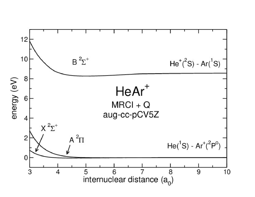
Figure 1: Potential energy curves for the X${}^{2}\Sigma^{+}$, A${}^{2}\Pi$ and B${}^{2}\Sigma^{+}$ states of the HeAr⁺ molecular cation as a function of internuclear distance $R$ (in $a_{0}$). The results shown were obtained in the MRCI + Q approximation using the molpro quantum chemistry package of codes with aug-cc-pCV5Z basis sets for He and Ar.

Calculations of the $\textrm{X}\,{}^{2}\Sigma^{+}$ and $\textrm{A}\,{}^{2}\Pi$ PECs were given by (Olson & Liu, 1978; Gemein & Peyerimhoff, 1990; Staemmler, 1990), the last two including fine-structure for the $\textrm{A}\,{}^{2}\Pi$ state, and the $\textrm{X}\,{}^{2}\Sigma^{+}$, $\textrm{A}\,{}^{2}\Pi$, and $\textrm{B}\,{}^{2}\Sigma^{+}$ states were calculated by Liao et al. (1987), using a relativistic CI method, and by Gemein et al. (1990) using the MRD-CI method. A summary of earlier calculations is given by Viehland et al. (1991). Semi-empirical functions fitting the PECs are available (Siska, 1986; Viehland et al., 1991). The $\textrm{B}\,{}^{2}\Sigma^{+}$ state has a well depth of about 0.17 eV ($1375\;\textrm{cm}^{-1}$), while the $\textrm{X}\,{}^{2}\Sigma^{+}$ and $\textrm{A}\,{}^{2}\Pi$ states have very shallow potentials wells of the order tens of meV (Dabrowski et al., 1981; Liao et al., 1987; Viehland et al., 1991; Carrington et al., 1995). For the $\textrm{X}\,{}^{2}\Sigma^{+}$ state the well depth is $286\;\textrm{cm}^{-1}$, while for the two states comprising the $\textrm{A}\,{}^{2}\Pi$ (including fine structure) state the depths are $\leq 182\;\textrm{cm}^{-1}$.

Depending on the relative magnitude of the transition dipole moments for the $\textrm{B}\,{}^{2}\Sigma^{+}$–$\textrm{X}\,{}^{2}\Sigma^{+}$ and $\textrm{B}\,{}^{2}\Sigma^{+}$–$\textrm{A}\,{}^{2}\Pi$ transitions, qualitatively, we might expect a relatively large radiative charge transfer rate coefficient because the $\textrm{B}\,{}^{2}\Sigma^{+}$ state is relatively shallow, the Franck-Condon overlap factors governing matrix elements for transitions between the $\textrm{B}\,{}^{2}\Sigma^{+}$ state and between the $\textrm{A}\,{}^{2}\Pi$ state and the $\textrm{X}\,{}^{2}\Sigma^{+}$ state are favorable, and the net energy between the initial and final states is $\sim 8$ eV, which enters the transition probability as a cubic factor. To our knowledge the transition dipole moments coupling the $\textrm{B}\,{}^{2}\Sigma^{+}$ and $\textrm{X}\,{}^{2}\Sigma^{+}$ states and the $\textrm{B}\,{}^{2}\Sigma^{+}$ and $\textrm{A}\,{}^{2}\Pi$ states are not available in the literature, so we calculated them using the latest version of the quantum chemistry package molpro, running on parallel computer architectures. The present results, described in more detail below, are shown in Fig. 2.

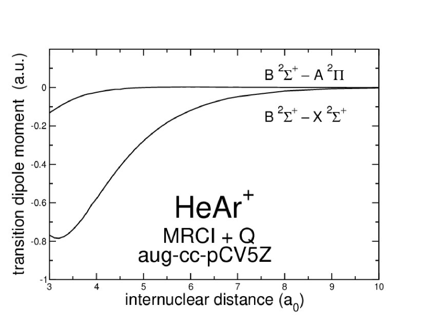
Figure 2: Transition dipole moments for the B${}^{2}\Sigma^{+}$–A${}^{2}\Pi$ and B${}^{2}\Sigma^{+}$–X${}^{2}\Sigma^{+}$ transitions in atomic units (a.u.) for the HeAr⁺ molecular cation as a function of internuclear distance $R$ (in $a_{0}$).

Inspection of the calculated transition dipole moments indicates that the leading channel for radiative charge transfer will be the $\textrm{B}\,{}^{2}\Sigma^{+}$–$\textrm{X}\,{}^{2}\Sigma^{+}$ transition in comparison to the $\textrm{B}\,{}^{2}\Sigma^{+}$–$\textrm{A}\,{}^{2}\Pi$ transition, similarly to the case of radiative charge transfer between $\textrm{He}^{+}$ and Ne (Liu et al., 2010).

Potential energy curves (PECs) and transition dipole moments (TDMs) as a function of internuclear distance $R$ were calculated for a range of values of internuclear distance $R$ between 3 and $60\;a_{0}$. We used a state-averaged-multi-configuration-self-consistent-field (SA-MCSCF) approach, followed by multi-reference configuration interaction (MRCI) calculations together with the Davidson correction (MRCI+Q) (Helgaker et al., 2000), in a similar manner to our recent molecular structure work on the HeC⁺ and the CH⁺ molecular complexes (Babb & McLaughlin, 2017b, a). The SA-MCSCF method is used as the reference wave function for the MRCI calculations. All the molecular data were obtained with molpro 2015.1 (Werner et al., 2015) in the C_2v Abelian symmetry point group using augmented - correlation - consistent polarized core-valence quintuplet basis sets (aug-cc-pCV5Z) for each atom/ion, in the MRCI+Q calculations (Helgaker et al., 2000). The use of large basis sets in molecular electronic structure calculations are well known to recover $\approx$ 98% of the electron correlation effects.

In detail, for the $\textrm{HeAr}^{+}$ molecular cation, thirteen molecular orbitals (MOs) are put into the active space, including seven $a_{1}$, three $b_{1}$ and three $b_{2}$ symmetry MOs. The rest of the electrons in the $\textrm{HeAr}^{+}$ system are put into the closed-shell orbitals. The MOs for the MRCI procedure are obtained from the SA-MCSCF method, where the averaging process was carried out on the lowest four ${}^{2}\Sigma^{+}$ (${}^{2}A_{1}$), four ${}^{2}\Pi$ (${}^{2}B_{1}$), and four ${}^{2}\Delta$ (${}^{2}A_{2}$) molecular states of this molecule. We then use these thirteen MOs (7$a_{1}$, 3$b_{1}$, 3$b_{2}$, 0$a_{2}$), i.e. (7,3,3,0), to perform all the PEC calculations of these electronic states in the MRCI + Q approximation as a function of bond length. The potential energies (PECs) and transition dipole moments (TDMs), respectively, are shown in Figs. 1 and 2, for the restricted range $3<R<10\;a_{0}$.

The long-range form of the $\textrm{B}\,{}^{2}\Sigma^{+}$ state potential energy, correlating to $\textrm{He}^{+}({}^{2}S_{0})$-$\textrm{Ar}({}^{1}S_{0})$, is (in atomic units)

$$V_{B}(R)\sim-\textstyle{\frac{1}{2}}\alpha(\textrm{Ar})R^{-4}-\frac{1}{2}\alpha_{q}(\textrm{Ar})R^{-6}-C_{6}(\textrm{He}^{+}\cdot\textrm{Ar})R^{-6},$$ (4)

where the electric dipole and quadrupole polarizabilities of Ar and the dispersion (van der Waals) constant of $\textrm{He}^{+}\cdot\textrm{Ar}$ are, respectively, $\alpha(\textrm{Ar})=11.08$ (Kumar & Thakkar, 2010), $\alpha_{q}(\textrm{Ar})=52.8$ (Jiang et al., 2015), and $C_{6}=2.36$. We calculated $C_{6}$ using the oscillator strength distributions (Babb, 1994) of $\textrm{He}^{+}$ (Johnson et al., 1967) and of Ar (Kumar & Thakkar, 2010). [The present value of $\frac{1}{2}\alpha_{q}(\textrm{Ar})+C_{6}(\textrm{He}^{+}\cdot\textrm{Ar})=28.8$ and is in good agreement with value 27.6 given by Siska (1986), who estimated $C_{6}$ using the Slater-Kirkwood approximation.]

The long-range forms of the $\textrm{X}\,{}^{2}\Sigma^{+}$ and $\textrm{A}\,{}^{2}\Pi$ states, correlating to $\textrm{He}(1s^{2}\;{}^{1}\textrm{S})$-$\textrm{Ar}^{+}(3p^{5}\;{}^{2}\textrm{P}^{\mathrm{o}})$, are (in atomic units)

$$V_{A;X}(R)\sim-\textstyle{\frac{1}{2}}\alpha(\textrm{He})R^{-4}-8.64R^{-6},$$ (5)

where the electric dipole polarizability of He is $\alpha(\textrm{He})=1.383$ (Yan et al., 1996) and the term ${\cal O}(R^{-6})$ is an estimate of the contribution of the electric quadrupole polarizability of helium and the dispersion constant for $\textrm{He}\cdot\textrm{Ar}^{+}$ (Siska, 1986; Carrington et al., 1995). The transition dipole moments are fitted to the form ${R}^{-12}$ for $R>16\;a_{0}$.

The calculated $\textrm{B}\,{}^{2}\Sigma^{+}$ potential gives a well of depth $D_{e}=0.03132$ eV $(2526\;\textrm{cm}^{-1})$ at $R=5\;a_{0}$, to be compared to the experimentally determined well depth of $1375\;\textrm{cm}^{-1}$ at the same value of $R$ (Dabrowski et al., 1981). Part of this discrepancy may be due to our neglect of fine structure (spin-orbit coupling), as shown for the $\textrm{X}\,{}^{2}\Sigma^{+}$ and $\textrm{A}\,{}^{2}\Pi$ states by Staemmler (1990).

3 Cross sections and rate coefficients

The radiative loss cross sections were calculated using the optical potential approach, which accounts for radiative loss in collisions of $\textrm{He}^{+}$ with Ar. The theory is described in Babb & McLaughlin (2017b), see also, for example, Zygelman & Dalgarno (1988); Liu et al. (2009) and references therein. In carrying out the calculations of (3), the probability of approach in the $\textrm{B}\,{}^{2}\Sigma^{+}$ state is unity. The reduced mass of the colliding system corresponds to ${}^{4}\textrm{He}$ and ${}^{36}\textrm{Ar}$.

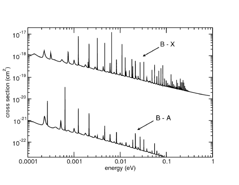
Figure 3: Cross sections in $\textrm{cm}^{2}$ for radiative loss in collisions of $\textrm{He}^{+}$ with Ar. Upper curve for $\textrm{B}\,{}^{2}\Sigma^{+}$ to $\textrm{X}\,{}^{2}\Sigma^{+}$ transitions, lower curve for $\textrm{B}\,{}^{2}\Sigma^{+}$ to $\textrm{A}\,{}^{2}\Pi$ transitions.

The calculated cross sections for radiative loss (radiative charge transfer) are shown in Fig. 3. As expected, the $\textrm{B}\,{}^{2}\Sigma^{+}$ to $\textrm{X}\,{}^{2}\Sigma^{+}$ transition is significantly larger than the $\textrm{B}\,{}^{2}\Sigma^{+}$ to $\textrm{A}\,{}^{2}\Pi$ transition. The radiative loss cross sections include the possibility of radiative association; however, because the well depth of the $\textrm{X}\,{}^{2}\Sigma^{+}$ state is only 262 $\textrm{cm}^{-1}$ and the well depth of the $\textrm{A}\,{}^{2}\Pi$ state is even less (Dabrowski et al., 1981; Carrington et al., 1995), and because the transition dipole moments are diminished at the equilibrium distances characteristic of these states (about $5\;a_{0}$), the relative contributions of radiative association to radiative loss are assumed to be very small. Cross sections for loss through radiative association from the initial $\textrm{B}\,{}^{2}\Sigma^{+}$ state to bound levels of the $\textrm{B}\,{}^{2}\Sigma^{+}$ state are also insignificant compared to the cross sections given in Fig. 3 because the transition probabilities depend on the de-excitation energies to the third power (Zygelman et al., 2014). Earlier detailed calculations on the $\textrm{LiHe}^{+}$ system are illustrative (Dalgarno et al., 1996; Stancil & Zygelman, 1996), in particular, Figure 2 of Augustovičová et al. (2012).

We therefore take the radiative loss cross section as a good approximation for the radiative charge transfer cross section. This is in contrast to the $\textrm{HeNe}^{+}$ system, where the well depth of the ground state is $D_{e}=6216\pm 300\;\textrm{cm}^{-1}$ and the transition dipole moments ($\textrm{B}\,{}^{2}\Sigma^{+}$–$\textrm{X}\,{}^{2}\Sigma^{+}$ and $\textrm{B}\,{}^{2}\Sigma^{+}$–$\textrm{A}\,{}^{2}\Pi$) are comparable, with roughly equal contributions to radiative loss from radiative charge transfer and from radiative association (Cooper et al., 1984; Liu et al., 2009). We note that cross sections for the various transitions that originate from the excited doublet electronic state of HeAr⁺ have Langevin $1/v$ (or $E^{-1/2}$), where $v$ is the relative velocity (and $E$ is the relative kinetic energy), background dependences at low energies, with overlying resonance features. The rate coefficients for process (3) were calculated by averaging the cross sections for the $\textrm{B}\,{}^{2}\Sigma^{+}$–$\textrm{X}\,{}^{2}\Sigma^{+}$ transition over a Maxwellian velocity distribution. The results are given in Table 1.

To check the sensitivity of the cross sections to the description of the $\textrm{B}\,{}^{2}\Sigma^{+}$ state, we repeated the calculations with the empirically determined $\textrm{B}\,{}^{2}\Sigma^{+}$ potential of Siska (1986), which reproduces the experimental well depth. The main effect of using the empirical $\textrm{B}\,{}^{2}\Sigma^{+}$ state potential was to change the positions of the resonances in the cross section at low energies, but this did not appreciably affect the values of the rate coefficients at thermal energies. We verified that the $\textrm{B}\,{}^{2}\Sigma^{+}$ to $\textrm{X}\,{}^{2}\Sigma^{+}$ cross sections shown in Fig. 3 satisfied the alternative upper bound for radiative charge transfer cross sections given in Eq. (A.6) of (Zygelman et al., 2014). The upper bound was consistently larger; by about 4% at energy $9\times 10^{-4}$ eV increasing to about 9% at energy 0.09 eV.

Table 1: Rate coefficients ($\textrm{cm}^{3}/\textrm{s}$) for radiative charge transfer in collisions of $\textrm{He}^{+}$ with Ar. Numbers in parentheses represent powers of 10 by which the preceding number should be multiplied.

Temperature	Rate coefficient
K	$\textrm{cm}^{3}/\textrm{s}$
77	1.05($-$14)
100	1.05($-$14)
200	1.01($-$14)
300	9.86($-$15)
400	9.69($-$15)
500	9.56($-$15)
600	9.48($-$15)
700	9.39($-$15)
800	9.32($-$15)
900	9.28($-$15)
1000	9.30($-$15)
2000	8.89($-$15)
3000	8.33($-$15)

4 Discussion

The calculated cross sections and rate coefficients are somewhat larger than those for radiative charge transfer between $\textrm{He}^{+}$ and Ne. For example, for radiative charge transfer of $\textrm{He}^{+}$ and Ne at 300 K experiment gives $1.0(3)\times 10^{-15}\;\textrm{cm}^{3}/\textrm{s}$ (Johnsen, 1983) to be compared with the theoretical value of about $5\times 10^{-16}\;\textrm{cm}^{3}/\textrm{s}$ (Cooper et al., 1984; Liu et al., 2009), while for radiative charge transfer of $\textrm{He}^{+}$ and Ar, we find a rate coefficient of $9.86\times 10^{-15}\;\textrm{cm}^{3}/\textrm{s}$. Similarly, at 77 K Johnsen (1983) measured a rate coefficient $\sim 2\times 10^{-15}\;\textrm{cm}^{3}/\textrm{s}$ for radiative charge transfer of $\textrm{He}^{+}$ and Ne and Liu et al. (2009) calculate $3\times 10^{-16}\;\textrm{cm}^{3}/\textrm{s}$, while at the same temperature for $\textrm{He}^{+}$ and Ar we find a rate coefficient of $1.05\times 10^{-14}\;\textrm{cm}^{3}/\textrm{s}$. The larger calculated values for the rate coefficients in the Ar system, compared to the calculated values for the Ne system, arise from two opposing effects. The dissociation limit of the $\textrm{B}\,{}^{2}\Sigma^{+}$ state is about 8.225 eV above the $\textrm{X}\,{}^{2}\Sigma^{+}$ state for $\textrm{HeAr}^{+}$ and compared to about 3.125 eV for $\textrm{HeNe}^{+}$, while the transition dipole moment of the dominant $\textrm{B}\,{}^{2}\Sigma^{+}$ to $\textrm{X}\,{}^{2}\Sigma^{+}$ transition in $\textrm{HeNe}^{+}$ (Cooper et al., 1984; Liu et al., 2009) is slightly larger than that for $\textrm{HeAr}^{+}$.

However, the rate coefficient for process (3) is probably not large enough to be a significant factor in the production of $\textrm{ArH}^{+}$ in the diffuse interstellar medium. The corresponding radiative charge transfer reaction has been added to the chemical network relevant to the $\textrm{ArH}^{+}$ molecular ion, as described in Neufeld & Wolfire (2016) in the PDRLight version of the Meudon PDR code (Le Bourlot, J. et al., 2012). The model was run both for diffuse galactic cloud conditions (standard interstellar radiation field, $n_{\mathrm{H}}=50\;\textrm{cm}^{-3}$, $T=50$ K, low visual extinction, cosmic ionization rate $\zeta=10^{-16}\;\textrm{s}^{-1}$) and for conditions corresponding to the Crab Nebula environment as reported in (Priestley et al., 2017) ($n_{\mathrm{H}}=2000\;\textrm{cm}^{-3}$, $\zeta=10^{–9}\;\textrm{s}^{-1}$). Using the value $10^{-14}\;\textrm{cm}^{3}/\textrm{s}$ for the rate coefficient of the radiative charge transfer reaction (3), no significant modifications of the chemical equilibrium of the $\textrm{ArH}^{+}$ molecular ion were found for either case.

References

- Albat & Wirsam (1977) Albat, R., & Wirsam, B. 1977, J. Phys. B: At. Mol. Phys., 10, 81
- Augustovičová et al. (2012) Augustovičová, L., Špirko, V., Kraemer, W. P., & Soldán, P. 2012, Chem. Phys. Lett., 531, 59
- Babb & McLaughlin (2017a) Babb, J., & McLaughlin, B. M. 2017a, MNRAS, 468, 2052
- Babb & McLaughlin (2017b) —. 2017b, J Phys B: At. Mol. Opt. Phys, 50, 044003
- Babb (1994) Babb, J. F. 1994, Molec. Phys., 81, 17
- Barlow et al. (2013) Barlow, M. J., Swinyard, B. M., Owen, P. J., et al. 2013, Science, 342, 1343
- Carrington et al. (1995) Carrington, A., Leach, C. A., Marr, A. J., et al. 1995, J. Chem. Phys., 102, 2379
- Cooper et al. (1984) Cooper, D. L., Kirby, K., & Dalgarno, A. 1984, Can. J. Phys., 62, 1622
- Dabrowski et al. (1981) Dabrowski, I., Herzberg, G., & Yoshino, K. 1981, J. Molec. Spect., 89, 491
- Dalgarno et al. (1996) Dalgarno, A., Kirby, K., & Stancil, P. C. 1996, ApJ, 458, 397
- Fehsenfeld et al. (1966) Fehsenfeld, F. C., Schmeltekopf, A. L., Goldan, P. D., Schiff, H. I., & Ferguson, E. E. 1966, J. Chem. Phys., 44, 4087
- Gemein et al. (1990) Gemein, B., de Vivie, R., & Peyerimhoff, S. D. 1990, J. Chem. Phys., 93, 1165
- Gemein & Peyerimhoff (1990) Gemein, B., & Peyerimhoff, S. D. 1990, Chem. Phys. Lett., 173, 7
- Helgaker et al. (2000) Helgaker, T., Jørgensen, P., & Olsen, J. 2000, Molecular Electronic-Structure Theory (New York, USA: Wiley)
- Hester (2008) Hester, J. J. 2008, ARA&A, 46, 127
- Isler (1974) Isler, R. C. 1974, Phys. Rev. A, 10, 117
- Jenkins (2013) Jenkins, E. B. 2013, ApJ, 764, 25
- Jiang et al. (2015) Jiang, J., Mitroy, J., Cheng, Y., & Bromley, M. W. J. 2015, At. Data Nucl. Data Tables, 101, 158
- Johnsen (1983) Johnsen, R. 1983, Phys. Rev. A, 28, 1460
- Johnsen et al. (1973) Johnsen, R., Leu, M. T., & Biondi, M. A. 1973, Phys. Rev. A, 8, 1808
- Johnson et al. (1967) Johnson, R. E., Epstein, S. T., & Meath, W. J. 1967, J. Chem. Phys., 47, 1271
- Jones et al. (1979) Jones, J. D. C., Lister, D. G., & Twiddy, N. D. 1979, J. Phys. B: At. Molec. Phys., 12, 2723
- Kumar & Thakkar (2010) Kumar, A., & Thakkar, A. J. 2010, J. Chem. Phys., 132, 074301
- Le Bourlot, J. et al. (2012) Le Bourlot, J., Le Petit, F., Pinto, C., Roueff, E., & Roy, F. 2012, A&A, 541, A76
- Liao et al. (1987) Liao, M. Z., Balasubramanian, K., Chapman, D., & Lin, S. H. 1987, Chem. Phys., 111, 423
- Liu et al. (2009) Liu, C. H., Qu, Y. Z., Wang, J. G., Li, Y., & Buenker, R. J. 2009, Phys. Lett. A, 373, 3761
- Liu et al. (2010) Liu, X. J., Qu, Y. Z., Xiao, B. J., et al. 2010, Phys. Rev. A, 81, 022717
- Müller et al. (2015) Müller, H. S. P., Muller, S., Schilke, P., et al. 2015, A&A, 582, L4
- Neufeld & Wolfire (2016) Neufeld, D. A., & Wolfire, M. G. 2016, ApJ, 826, 183
- Olson & Liu (1978) Olson, R. E., & Liu, B. 1978, Chem. Phys. Lett., 56, 537
- Priestley et al. (2017) Priestley, F. D., Barlow, M. J., & Viti, S. 2017, MNRAS, 472, 4444
- Roueff et al. (2014) Roueff, E., Alekseyev, A. B., & Le Bourlot, J. 2014, A&A, 566, A30
- Sankrit et al. (1998) Sankrit, R., Hester, J. J., Scowen, P. A., et al. 1998, ApJ, 504, 344
- Schilke et al. (2014) Schilke, P., Neufeld, D. A., Müller, H. S. P., et al. 2014, A&A, 566, A29
- Siska (1986) Siska, P. E. 1986, J. Chem. Phys., 85, 7497
- Smith et al. (1970) Smith, F. T., Fleischmann, H. H., & Young, R. A. 1970, Phys. Rev. A, 2, 379
- Staemmler (1990) Staemmler, V. 1990, Z. Phys. D, 16, 167
- Stancil & Zygelman (1996) Stancil, P. C., & Zygelman, B. 1996, ApJ, 472, 102
- Stärk & Peyerimhoff (1986) Stärk, D., & Peyerimhoff, S. D. 1986, Molec. Phys., 59, 1241
- Viehland et al. (1991) Viehland, L. A., Viggiano, A. A., & Mason, E. A. 1991, J. Chem. Phys., 95, 7286
- Werner et al. (2015) Werner, H.-J., Knowles, P. J., Knizia, G., et al. 2015, molpro, version 2015.1, a package of ab initio programs, Cardiff, UK, see http://www.molpro.net
- Yan et al. (1996) Yan, Z.-C., Babb, J. F., Dalgarno, A., & Drake, G. W. F. 1996, Phys. Rev. A, 54, 2824
- Zygelman & Dalgarno (1988) Zygelman, B., & Dalgarno, A. 1988, Phys. Rev. A, 38, 1877
- Zygelman et al. (2014) Zygelman, B., Lucic, Z., & Hudson, E. R. 2014, J. Phys. B: At. Mol. Opt. Phys., 47, 015301