Investigation of surface boundary conditions for continuum modeling of RF plasmas

Abstract

This work was motivated by a lacking general consensus in the exact form of the boundary conditions (BCs) required on the solid surfaces for the continuum modeling of RF plasmas. Various kinds of number and energy density BCs on solid surfaces were surveyed and how they interacted with the electric potential BC to affect the plasma was examined in two fundamental RF plasma reactor configurations. A second-order local mean energy approximation with equations governing the electron and ion number densities, and the electron energy density was used to model the plasmas. Zero densities and various combinations of drift, diffusion and thermal fluxes were considered to set up BCs. It was shown that the choice of BC can have a significant impact on the sheath and bulk plasma. The thermal and diffusion fluxes to the surface were found to be important. A pure drift BC for dielectric walls failed to produce a sheath.

I Introduction

Radiofrequency (RF) plasmas are encountered in many situations of practical interest such as manufacturing processes and laboratory experiments. RF plasmas are used for etching and deposition of thin films on semiconductors, plasma enhanced chemical vapor deposition (PECVD) Stoffel1996 , producing quantum dots Michalet2005 , plasma synthesis Pi2008 , coating nanoparticles Cao2002 , and producing carbon nanotubes Meyyappan2003 . They are also used in some dusty plasma experiments Shukla2001 where phenomena such as Coulomb crystallization Ikezi1986 ; Schweigert1996 and dust charging Matthews2011 ; Havnes1990 are examined and in plasma medicine applications ranging from equipment sterilization Moisan2001 ; Laroussi2005 to wound healing Fridman2008 and possibly cancer treatment Schlegel2013 . Modeling through continuum (hydrodynamic) approaches has been an essential tool in understanding RF plasmas in both basic and applied research setups Park1990 ; Goedheer2004 ; Parent2014 ; Zakari2015 .

In the continuum modeling of plasmas, partial differential equations derived from the first two or three moments of the Boltzmann equation are solved. There are two common continuum models for RF plasmas. One is based on the local field approximation where a set of drift-diffusion equations describing the time and space variations of the ion and electron number densities are solved Barnes1987 ; Grubert2009 . The other is based on the local mean energy approximation where an additional drift-diffusion equation is solved for the electron energy Graves1986 ; Gogolides1992 ; Hammond2002 . In both approaches, a poisson equation is solved for the electric potential.

Although boundary conditions (BC’s) are essential for continuum modeling, what constitutes an adequate BC on the solid surfaces of an RF plasma is not completely described in the literature. Continuum models for RF plasmas conventionally use the same boundary conditions as DC plasmas. There has been some detailed studies focused on the BC’s for direct current glow discharges Hagelaar2000BC ; Surzhikov2004 ; however, the competence of these conditions for RF plasmas has not been thoroughly investigated. In general, RF plasma continuum models use the local-mean-energy approximation which requires solving the electron energy equation. In contrast, DC plasmas often use the local-field-approximation which neglects the electron energy equation, hence the energy boundary conditions are not included Hagelaar2000BC ; Surzhikov2004 . Moreover, DC plasma boundary conditions often include the secondary electron emission (SEE) due to ion impact on the surfaces Hagelaar2000BC ; Bouanaka2013 whereas RF plasmas often neglect it.

A continuum plasma model requires a set of BC’s for the number and energy densities, and a BC for the electric potential. For the electric potential, surfaces are often grounded or have a known voltage, but could instead be dielectrics Boeuf1995 ; Davoudabadi2007 where the surface develops a non-uniform charge as a result of the current from the plasma. The number and energy densities are set to zero at the surface in some studies Passchier1993 ; Davoudabadi2009 on the assumption that the charged particles are absorbed by the surface. In other studies, the flux to the surface is specified based on the drift toward the boundary Davoudabadi2007 ; Horn2011 and the thermal motion Boeuf1995 ; Paunska2011 . The SEE effects at boundaries are often neglected in RF discharges although occasionally they are included Gozadinos2003 .

In the works reviewed above, the rationale for selecting the BC kind is rarely provided and the importance of the choice is not fully discussed or quantified. The current work examines and compares various boundary conditions for the number and energy densities and determines their effects in two fundamental RF plasma setups. The differential equations of the continuum model used here are presented in Sec. II. The details of the boundary conditions are discussed in Sec. III. The numerical methods used to solve the system of equations are illustrated in Sec. IV. The results are discussed in Sec. V and conclusions are made in Sec. VI.

II Governing Equations

The second-order ‘local mean energy’ model Gogolides1992 is used for the RF plasmas studied in this work. In this model, the equations governing the electron number density $n_{e}$, ion number density $n_{i}$, and electron energy density $\omega_{e}$ are:

$$\frac{\partial n_{e(i)}}{\partial t}+\bm{\nabla}\cdot\bm{\Gamma}_{e(i)}=S_{e(i)},$$ (1)

$$\frac{\partial\omega_{e}}{\partial t}+\bm{\nabla}\cdot\bm{\Gamma}_{\omega}=-e\bm{\Gamma}_{e}\cdot\bm{E}+S_{\omega},$$ (2)

where

$$\bm{\Gamma}_{e(i)}=\text{sgn}(q)n_{e(i)}\mu_{e(i)}\bm{E}-D_{e(i)}\bm{\nabla}n_{e(i)},$$ (3)

$$\bm{\Gamma}_{\omega}=\frac{5}{3}\left(-\omega_{e}\mu_{e}\bm{E}-D_{e}\bm{\nabla}\omega_{e}\right),$$ (4)

and $\text{sgn}(q)$ is 1 for ions and -1 for electrons and electron energy. Here, $\bm{E}$ is the electric field calculated by:

$$\bm{E}=-\bm{\nabla}\phi,$$ (5)

where $\phi$ is the electric potential which satisfies Poisson’s equation:

$$\nabla^{2}\phi=\frac{e}{\epsilon_{0}}\left(n_{e}-n_{i}\right),$$ (6)

where $e$ is the electron charge. In the equations above, $\mu_{e(i)}$ is the electron (ion) mobility, $D_{e(i)}$ is the electron (ion) diffusion coefficient and $\bm{E}$ is the electric field. Eqs. (3-4) define the fluxes of electrons (ions) and energy, respectively. The source term $S_{e(i)}$ in eq. (1) accounts for the electrons and ions created by ionization. The gas is assumed to be singly ionized, therefore $S_{i}=S_{e}=k_{i}n_{e}n_{\text{gas}}$ where $k_{i}$ is the ionization rate coefficient. The ionization rate was determined by BOLSIG+ Hagelaar2005 which solves the electron Boltzmann equation and tabulates the ionization rate and excitation rates as a function of the mean electron energy. The mean electron energy $\varepsilon$, the electron temperature $T_{e}$ and $\omega_{e}$ are correlated with each other through

$$\omega_{e}=n_{e}\varepsilon=\frac{3}{2}k_{B}n_{e}T_{e},$$ (7)

where $k_{B}$ is the Boltzmann constant. In the energy equation (2), the term $-e\bm{\Gamma}_{e}\cdot\bm{E}$ accounts for the ohmic or joule heating of the electrons in the electric field and the term $S_{\omega}=S_{e}H_{i}$ accounts for the energy loss due to ionization and excitation, where $H_{i}$ is the ionization energy.

III Boundary Conditions

There are three kinds of boundary conditions which are used in plasma modeling: the variable is specified at the boundary (Dirichlet kind), the normal component of the gradient of the variable is specified at the boundary (Neumann kind), or the flux, given by eqs. (3-4) which is a function involving the variable and its gradient, is specified at the boundary (Robin kind). Extrapolation boundary conditions can also be used, although they are typically used for outflows not solid surfaces.

III.1 Electric potential boundary conditions

The BC for Poisson’s equation can be either a Dirichlet kind where the voltage is specified or a Neumann kind where the normal component of the electric field is specified. In this study, a specified voltage condition is used for the electrodes, which are assumed to be conductors, and a specified electric field condition is used for lateral walls, which are assumed to be dielectrics.

III.1.1 Specified voltage (Dirichlet)

In the most common configuration for an RF plasma, one electrode has an applied voltage and the other electrode is grounded. Sometimes the outer wall of the reactor will also be grounded Passchier1993 . For a grounded surface, the boundary condition is:

$$\phi=0.$$ (8)

For the powered electrode, the electric potential is given by:

$$\phi=V_{\text{DC}}+V_{\text{RF}}\sin\left(2\pi ft\right),$$ (9)

where $V_{\text{DC}}$ is the direct current voltage, $V_{\text{RF}}$ is the radiofrequency voltage and $f$ is the RF frequency. In one-dimensional cases, the direct current voltage will be zero, however, for two or three-dimensional cases, there can be a difference in the area of the powered electrode and the total grounded area, which causes a natural DC bias Passchier1993 ; Land2009 . In the case of a cylindrical reactor where the outer wall is a dielectric, the DC bias will be zero.

III.1.2 Dielectric (Neumann)

Another common BC for the electric potential is a dielectric surface Boeuf1995 ; Davoudabadi2007 . In this kind, the electric field (gradient of the potential) is imposed through a equation using the wall charge. The charge density distribution $\sigma$ is the time integral of the current to the wall so for a singly ionized gas, this equation reads:

$$\frac{\partial\sigma}{\partial t}=e\left(\bm{\Gamma}_{i}-\bm{\Gamma}_{e}\right)\cdot\bm{n},$$ (10)

where $\bm{n}$ is the unit normal vector directed out of the domain on the boundary surface. The electric field is correlated with the wall charge through Gauss’ law:

$$-\bm{E}\cdot\bm{n}=\frac{\sigma}{\epsilon_{0}}.$$ (11)

III.2 Number and energy density boundary conditions

The BCs for the number and electric energy equations are either a Dirichlet kind where the number and energy density are specified, or a Robin kind, where the fluxes are specified. There is no general consensus in the literature on how to specify the fluxes. Secs. III.2.2 through III.2.5 discusses the flux boundary conditions used in the previous studies.

III.2.1 Zero densities (Dirichlet)

The simplest BC assumes that the surface is perfectly absorbing with no reflection Passchier1993 ; Davoudabadi2009 , therefore, the ion and electron number density at the surface are zero, i.e., $n_{i}=n_{e}=0$, and correspondingly, $\omega_{e}=0$. In a variant form of these BCs, the component of ion density gradient normal to the wall is set to zero, i.e., $\bm{\nabla}n_{i}\cdot\bm{n}=n_{e}=\omega_{e}=0$ Surendra1990 . If the electric field is directed out of the domain causing the ions to flow out of the domain, the zero ion density gradient boundary condition produces the same results as the zero number density boundary condition. This is the case for the plasmas examined in this study so the zero gradient condition is not included here.

III.2.2 Pure drift (Robin)

In this BC, the flux directed towards the surface is assumed pure drift with no diffusion and no flux away from the surface Davoudabadi2007 ; Horn2011 . It is necessary to determine whether the flux is towards the surface, which can be accomplished by defining:

$${}a_{e(i)}=\left\{\begin{array}[]{cc}1&\text{sgn}(q)\bm{E}\cdot\bm{n}\geq 0\\ 0&\text{sgn}(q)\bm{E}\cdot\bm{n}<0\end{array}\right..$$ (12)

The normal component of the electron (ion) flux at the boundary is:

$$\bm{\Gamma}_{e(i)}\cdot\bm{n}=\left[a_{e(i)}\text{ sgn}(q)\mu_{e(i)}\bm{E}\cdot\bm{n}\right]n_{e(i)},$$ (13)

where $\bm{\Gamma}_{e(i)}$ is given in eq. (3). Correspondingly, the normal component of the energy flux is calculated by:

$$\bm{\Gamma}_{\omega}\cdot\bm{n}=\left[-a_{e}\frac{5}{3}\mu_{e}\bm{E}\cdot\bm{n}\right]\omega_{e}.$$ (14)

III.2.3 Thermal flux (Robin)

In this BC Boeuf1995 ; Paunska2011 , the flux directed towards the surface is a combination of the drift flux to the surface, as in Section III.2.2, and the thermal flux towards the surface. As a result, there is always flux towards the surface even when the electric field causes the drift to be directed away from the surface. The thermal flux towards the surface is assumed to be the one-way flux for a Maxwellian distribution which is equal to $\frac{1}{4}nv_{\text{th}}$. For the ions and electrons, the flux at the boundary is:

$$\bm{\Gamma}_{e(i)}\cdot\bm{n}=\left[a_{e(i)}\text{ sgn}(q)\mu_{e(i)}\bm{E}\cdot\bm{n}+\frac{1}{4}v_{\text{th}_{e(i)}}\right]n_{e(i)},$$ (15)

where $v_{\text{th}_{e(i)}}$ is the thermal velocity of the electrons (ions) determined by:

$$v_{\text{th}_{e(i)}}=\sqrt{\frac{8k_{B}}{\pi}\frac{T_{e(i)}}{m_{e(i)}}}.$$ (16)

With respect to the energy BC, there are two approaches, both of which can be formulated by

$$\bm{\Gamma}_{\omega}\cdot\bm{n}=\left[-a_{e}\frac{5}{3}\mu_{e}\bm{E}\cdot\bm{n}+\beta v_{\text{th}_{e}}\right]\omega_{e},$$ (17)

where $\beta$ is a factor depending on the approach. In the first approach, where the thermal flux is equated to the enthalpy flux Nitschke1994 ; Hammond2002 ; Bogdanov2013 , $\beta=5/12$ as the enthalpy flux is $\frac{5}{2}k_{B}T_{e}\bm{\Gamma}_{e}$. In the second approach, where the thermal flux is equated to the one-way flux of kinetic energy for a Maxwellian distribution Rafatov2012BC ; WenXia2013 ; Liu2014 ; Boeuf1995 , $\beta=1/3$ as the one-way flux of kinetic energy for a Maxwellian distribution is $2k_{B}T_{e}\bm{\Gamma}_{e}$. The one-way flux of kinetic energy for a Maxwellian distribution is more consistent with the assumptions made for the electron BC, therefore, the second approach is chosen here.

III.2.4 Thermal and diffusion flux (Robin)

This boundary condition assumes that in addition to the previously considered drift and thermal fluxes, the diffusion flux to the wall is significant. It is based on a formulation proposed by Hagelaar et al. Hagelaar2000BC , but the SEE coefficient is set to zero in order to determine the impact of the diffusion flux. The ion BC adds a diffusion term $\left(-\frac{1}{2}D_{i}\bm{\nabla}\cdot\bm{n}\right)$ to Eq. (15) giving:

$$\bm{\Gamma}_{i}\cdot\bm{n}=\left[a_{i}\mu_{i}\bm{E}\cdot\bm{n}+\frac{1}{4}v_{\text{th}_{i}}\right]n_{i}-\frac{1}{2}D_{i}\bm{\nabla}n_{i}\cdot\bm{n}.$$ (18)

The term involving the gradient can be challenging to implement due to possible numerical difficulties in evaluating the gradient, so Hagelaar et al. Hagelaar2000BC proposed an alternative form, using the definition of the ion flux in Eq. (3). This form for the electron (ion) flux reads:

$$\bm{\Gamma}_{e(i)}\cdot\bm{n}=\left[\text{sgn}(q)\left(2a_{e(i)}-1\right)\mu_{e(i)}\bm{E}\cdot\bm{n}+\frac{1}{2}v_{\text{th}}\right]n_{e(i)}.$$ (19)

Since the plasma model used by Hagelaar et al. Hagelaar2000BC did not include the electron energy equation, they did not discuss the BC for the energy equation. Here, the following condition, which is consistent with Eq. (18), is used for the energy flux of the electrons:

$$\bm{\Gamma}_{\omega}\cdot\bm{n}=\left[-a_{e}\frac{5}{3}\mu_{e}\bm{E}\cdot\bm{n}+\frac{1}{3}v_{\text{th}_{e}}\right]\omega_{e}-\frac{5}{6}D_{e}\bm{\nabla}\omega_{e}\cdot\bm{n}.$$ (20)

The last term accounts for the diffusion, the coefficient is $D_{\omega}/2$ which simplifies to $5D_{E}/6$ since $D_{\omega}=5D_{e}/3$, the other terms match Eq. (17) for the thermal flux boundary condition. Another equivalent alternative form without the gradient term is given by:

$$\begin{gathered}\bm{\Gamma}_{\omega}\cdot\bm{n}=\left[-\left(2a_{e}-1\right)\frac{5}{3}\mu_{e}\bm{E}\cdot\bm{n}+\frac{2}{3}v_{\text{th}}\right]\omega_{e}.\end{gathered}$$ (21)

III.2.5 Secondary electron emission (Robin)

This BC includes the effect of the SEE by ion impact. Here, the formulation given in the previous works Hagelaar2000BC ; Lee2012 ; Iqbal2014 are used to apply this BC. The ion flux at the boundary is identical to Eq. (19). On the other hand, the net electron density at the boundary is the combination of the density of SEE electrons, $n_{\gamma}$, and the density of primary electrons directed from the bulk, $n_{\alpha}=n_{e}-n_{\gamma}$. Therefore, the electron flux normal to the wall is given by $\bm{\Gamma}_{e}\cdot\bm{n}=\bm{\Gamma}_{\gamma}\cdot\bm{n}+\bm{\Gamma}_{\alpha}\cdot\bm{n}$, where $\bm{\Gamma}_{\gamma}$ is the flux of the SEE electrons and $\bm{\Gamma}_{\alpha}$ is the bulk electron flux. The BC for the bulk electron flux is similar to that for the ions:

$$\begin{gathered}\bm{\Gamma}_{\alpha}\cdot\bm{n}=\left[-\left(2a_{e}-1\right)\mu_{e}\bm{E}\cdot\bm{n}+\frac{1}{2}v_{\text{th}}\right]n_{\alpha}.\end{gathered}$$ (22)

On the other hand, the secondary electrons are assumed to have a beam-like behavior and not flow back to the wall, thus, the BC for the SEE flux is:

$$\bm{\Gamma}_{\gamma}\cdot\bm{n}=-\left(1-a_{e}\right)\gamma\bm{\Gamma}_{i}\cdot\bm{n},$$ (23)

where $\gamma$ is the SEE coefficient which defines the average number of electrons emitted per ion impact. Due to the beam-like behavior assumption for the emitted secondary electrons, they do not flow back towards the surface and diffusion can be neglected. Therefore, the number density of the secondary electrons can be written as:

$$n_{\gamma}=\left(1-a_{e}\right)\frac{\gamma\bm{\Gamma}_{i}\cdot\bm{n}}{\mu_{e}\bm{E}\cdot\bm{n}}.$$ (24)

From the equations above, the BC for the total electron flux is derived:

$$\begin{gathered}\bm{\Gamma}_{e}\cdot\bm{n}=\left[-\left(2a_{e}-1\right)\mu_{e}\bm{E}\cdot\bm{n}+\frac{1}{2}v_{\text{th}}\right]n_{e}\\ -\frac{1}{2}v_{\text{th}}n_{\gamma}-2\left(1-a_{e}\right)\gamma\bm{\Gamma}_{i}\cdot\bm{n}.\end{gathered}$$ (25)

The detail of this derivation is given in Appendix A. Eq. (25) is identical to the SEE BC equation used in the previous works  Hagelaar2000BC ; Lee2012 ; Iqbal2014 .

The energy density at the boundary consists of the SEE electron energy $\omega_{\gamma}$ and the bulk energy $\omega_{\alpha}=\omega_{e}-\omega_{\gamma}$. The energy flux of the electrons from the bulk is calculated by:

$$\begin{gathered}\bm{\Gamma}_{A}\cdot\bm{n}=\left[-\left(2a_{e}-1\right)\left(\frac{5}{3}\mu_{e}\right)\bm{E}\cdot\bm{n}+\frac{2}{3}v_{\text{th}}\right]\omega_{\alpha}.\end{gathered}$$ (26)

Due to the beam-like behavior assumed for the SEE electrons, the energy BC for the SEE electrons is:

$$\bm{\Gamma}_{B}\cdot\bm{n}=\left[-\left(1-a_{e}\right)\gamma\bm{\Gamma}_{i}\cdot\bm{n}\right]\varepsilon_{\gamma},$$ (27)

where $\varepsilon_{\gamma}$ is the mean energy that the secondary electrons are emitted at, which for this study is set to 2 eV Becker2013 . The energy density of the secondary electrons is calculated by:

$$\omega_{\gamma}=\left(1-a_{e}\right)\frac{\gamma\varepsilon_{\gamma}\bm{\Gamma}_{i}\cdot\bm{n}}{\mu_{e}\bm{E}\cdot\bm{n}}.$$ (28)

Using Eqs (26-28) and following a derivation procedure similar to the one given for the electron BC in Eq. (25), the following equation is derived for the energy BC:

$$\begin{gathered}\bm{\Gamma}_{\omega}\cdot\bm{n}=\left[-\left(2a_{e}-1\right)\frac{5}{3}\mu_{e}\bm{E}\cdot\bm{n}+\frac{2}{3}v_{\text{th}}\right]\omega_{e}\\ -\frac{2}{3}v_{\text{th}}\omega_{\gamma}-2\left(1-a_{e}\right)\varepsilon_{\gamma}\gamma\bm{\Gamma}_{i}\cdot\bm{n}.\end{gathered}$$ (29)

This equation is identical to that used by Lee et al. Lee2012 to set the energy BC.

III.3 Extrapolation boundary condition for ions

In the boundary conditions given in Sections III.2.1-III.2.5, the ions and electrons are dealt with at the boundary, similarly. However, Hammond et al Hammond2002 suggested that this treatment may not be appropriate because their analysis showed that ion boundary conditions were not necessary. Their analysis showed that the electric field was directed out of the plasma which meant the ions always flowed out of the domain. To set up a boundary condition consistent with the suggestion made by Hammond et al, cases were run in the current study with an extrapolation condition used for the ion number density when the electric field was directed out of the domain. In the extrapolation boundary condition, the value of the variable at the boundary is extrapolated from the values at the grid points near the boundary.

IV Numerical Method

A second order discretization scheme was applied on the time derivatives in the plasma equations:

$$\frac{3n_{e}^{n+1}-4n_{e}^{n}+n_{e}^{n-1}}{2\Delta t}+\bm{\nabla}\cdot\left(-\mu_{e}n_{e}^{n+1}\bm{E}^{n+1}-D_{e}\bm{\nabla}n_{e}^{n+1}\right)=S_{e}^{n},$$ (30)

$$\frac{3n_{i}^{n+1}-4n_{i}^{n}+n_{i}^{n-1}}{2\Delta t}+\bm{\nabla}\cdot\left(\mu_{i}n_{i}^{n+1}\bm{E}^{n+1}-D_{i}\bm{\nabla}n_{i}^{n+1}\right)=S_{e}^{n},$$ (31)

$$\begin{gathered}\frac{3\omega_{e}^{n+1}-4\omega_{e}^{n}+\omega_{e}^{n-1}}{2\Delta t}+\bm{\nabla}\cdot\frac{5}{3}\left(-\mu_{e}\omega_{e}^{n+1}\bm{E}^{n+1}-D_{e}\bm{\nabla}\omega_{e}^{n+1}\right)\\ =-e\bm{\Gamma}_{e}^{n+1}\cdot\bm{E}^{n+1}+S_{\omega}^{n},\end{gathered}$$ (32)

$$\nabla^{2}\phi^{n+1}=\frac{e}{\epsilon_{0}}\left(n_{e}^{n+1}-n_{i}^{n+1}\right),$$ (33)

where the superscript $n$ indicates the time level and the electric field comes from Eq. (5). The ionization source is treated as an explicit term. These equations constitute a nonlinear set of equations at time level $n+1$ for $n_{e}^{n+1}$, $n_{i}^{n+1}$, $\omega_{e}^{n+1}$, and $\phi^{n+1}$ after the spatial discretization is carried out. The nonlinearity is due to the nonlinear first terms in the parentheses of eqs. (30-32) on the left hand sides and the nonlinear first term on the right hand side of eq. (32). The equations are advanced in time by estimating the electric field at the new timestep, $\bm{E}^{n+1}$, then updating $n_{e}^{n+1}$, $n_{i}^{n+1}$, $\omega_{e}^{n+1}$ and finally the electric field is updated. Since $n_{e}$ is updated before $\omega_{e}$, the ohmic heating term in Eq. (32) uses the updated value of $n_{e}$. The equations are iterated until the system is solved simultaneously.

For the spatial discretization, a finite difference method is applied in an axisymmetric cylindrical coordinate consistent with the axisymmetric geometry of the plasma reactor studied in this work. The spatial discretization of the fluxes, the terms in the parentheses of eqs (30-33), uses the Scharfetter-Gummel scheme Scharfetter1969 ; Boeuf1987 ; Hagelaar2000 . For this scheme, the equation for the flux of $n$ in the y-direction is given by:

$$\begin{gathered}\Gamma_{j+1/2}=\frac{D}{\Delta y}\left[\frac{\text{Pe}}{1-\exp\left(-\text{Pe}\right)}n_{j}-\left(\frac{\text{Pe}}{1-\exp\left(-\text{Pe}\right)}-\text{Pe}\right)n_{j+1}\right],\end{gathered}$$ (34)

where Pe is the Peclet number, defined as:

$$\text{Pe}=\frac{\text{sgn}(q)\mu E_{y}\Delta y}{D}.$$ (35)

In the computations with very small values of $\mathrm{Pe}$, an expanded expression is used for $\frac{\mathrm{Pe}}{1-\exp\left(-\mathrm{Pe}\right)}=1+\mathrm{Pe}/{2}+{\mathrm{Pe}^{2}}/{12}-{\mathrm{Pe}^{4}}/{720}+\cdots$.

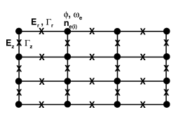
Figure 1: Staggered finite difference mesh: primary variables are stored at nodes (designated by $\bullet$) and fluxes and the electric field are stored at the midpoints (designated by $\times$).

A nonuniform, tan-stretched, grid is used with a higher resolution near the electrodes and outer wall. The grid is staggered, as shown in Fig. 1, with the primary variables, $\phi$, $n_{e,i}$, and $\omega_{e}$, evaluated on the nodes, j, and the electric field $\bm{E}$ and the fluxes $\bm{\Gamma}_{e,i,\omega}$ evaluated halfway between the nodes. The boundary passes through the nodes. For the boundary conditions where the flux to the surface is considered, the flux is specified at the midpoint between the boundary and the first interior node and the number and energy density at the boundary is obtained from Eq. (34).

V Results and Discussion

V.1 Validation of plasma model

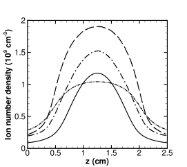
(a)

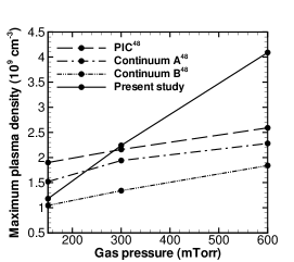
(b)

Figure 2: Validation of the continuum model used in the current study against the PIC and two continuum models A (DDAn) & B (DDA53) of Becker et al.Becker2017 for an argon plasma: (a) RF-averaged ion number density (in 10⁹ cm^-3) for a gas pressure of 150 mTorr; and (b) maximum plasma density (in 10⁹ cm^-3) as a function of gas pressure (in mTorr).

The plasma model was validated against the results of Becker et al. Becker2017 , who examined the differences between PIC/MCC and two continuum model simulations in a one dimensional reactor setup. The continuum model used here differs from their continuum models in the assumption of constant transport coefficients and the source of the ionization rate as well as the modeling of the ion flux. The models were compared at three different gas pressures, 150, 300, and 600 mTorr. Becker et al. specified the amplitude of the electrode current density as 10 $A/m^{2}$ which, for the PIC/MCC simulations, corresponded to voltage amplitudes of 90, 70, and 60V for the three pressures, respectively. Their continuum models produced different voltages as they matched the amplitudes of the current density. Here, we matched the voltage from their PIC/MCC simulations. Figure 2(a) shows the ion number density for a gas pressure of 150 mTorr and Fig. 2(b) shows the maximum plasma density as a function of gas pressure. The current model underpredicts the maximum plasma density by 40% compared to the PIC/MCC code at the lowest pressure but agrees well for the 300 mTorr case; the 60% difference for the 600 mTorr case is likely due to matching the voltage rather than the current. Since specifying the current to the electrodes, rather than the voltage, adds an additional complication to the boundary condition comparison, this study specifies the electrode voltage and does not attempt to compare the effect of the boundary conditions with PIC/MCC simulations.

To examine the impact of the boundary condition on the solution, an argon plasma was modeled using each of the number and energy density boundary conditions discussed in Section III.2. Two configurations of the plasma reactor were considered: a one-dimensional setup and an axisymmetric cylindrical one. Both the one-dimensional and cylindrical configurations had the RF voltage applied to the lower electrode while the upper electrode was grounded. The wall in the cylindrical configuration was dielectric meaning that the DC bias voltage discussed in Section III.1 is zero. The operating parameters are tabulated in Table 1. The mobility and diffusion coefficients were assumed constant.

Several cases were simulated with different sets of the BCs, as illustrated in Secs. III.2.1–III.2.5. For ease of reference, the number and energy boundary conditions are designated as shown in Table 2. All cases were simulated until a quasi-steady state was reached which is defined as the sate when the change in the RF-period averaged values was negligible. Here, BC4 is treated as the baseline case to which the other boundary conditions are compared.

V.2 One-dimensional configuration results

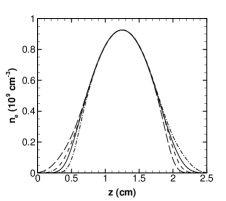
(a)

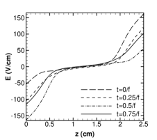
(b)

Figure 3: Spatial variation of (a) electron number density (in 10⁹ cm^-3); and (b) Electric field magnitude (in V/cm) at different times in the one-dimensional configuration

Figure 3 shows the spatial variation of the instantaneous electron number density and electric field at four different times during the RF period for BC4. All other cases exhibit qualitatively similar trends so the transient results are only shown for the BC4 case. Both electrodes have large sheaths, the time variation of the electron number density is significant in the region less than 0.75 cm from the electrode. The electric field is negative at the lower electrode, varying between -50 and -150 V/cm, and positive at the upper electrode, varying between 50 and 150 V/cm. This behavior indicates that the electric field is directed out of the domain through the entire RF cycle for both electrodes.

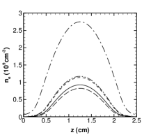
(a)

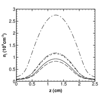
(b)

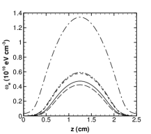
(c)

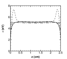
(d)

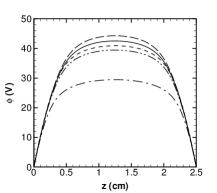
(e)

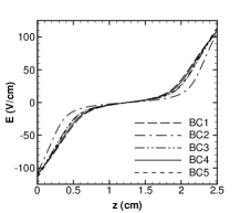
(f)

Figure 4: Spatial variation of RF-averaged plasma variables: (a) electron number density (in 10⁹ cm^-3); (b) ion number density (in 10⁹ cm^-3); (c) electron energy density (in 10¹⁰ eV cm^-3); (d) mean electron energy (in eV); (e) electric potential (in V); and (f) electric field magnitude (in V/cm) in the one-dimensional configuration.

Figure 4 shows the RF-averaged plasma variables for the different BC cases. As seen in Figs. 4(a) and 4(b), BC2 (the pure drift BC) has a substantially higher plasma density than the other BC kinds. This is due to the fact that the electric field is always pointing out of the domain so the electron BC uses a zero flux condition which results in a higher electron density at the boundary because the surface does not act as an electron sink. In a practical situation, flux towards the surface is always expected due to thermal motion and diffusion. It is seen that BC4 produces a lower plasma density than BC3, which is due to the lacking diffusion flux in BC3. The difference between BC4 and BC5 results in Fig. 4 is significant, showing a significant influence of the SEE mechanism for the considered SEE coefficient of 0.5.All cases produce a bulk mean electron energy of about 5eV. The case with SEE, BC5, shows a substantial increase in the mean energy in part of the sheath, which has been observed in other studies Lymberopoulos1993 as well.

In Section III.3, it was noted that there were potential concerns about the ion boundary condition due to the electric field causing the ions to flow out of the domain. Fig. 4(f) shows that all BC’s have the RF-averaged electric field directed out of the domain and Fig. 3(b) shows that the electric field is directed out of the domain throughout the RF period so both electrodes meet the criteria for setting the ion extrapolation boundary condition. However, when the ion BC was changed to the extrapolation condition, none of the cases experienced an appreciable impact in the bulk of the plasma. This change in the ion boundary condition only affected the ion number density on the boundary itself, the interior points were unaffected.

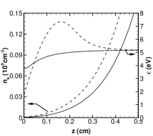
(a)

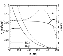
(b)

Figure 5: Spatial variation of electron number density (in 10⁹ cm^-3); and mean energy (in eV) for the (a) lower sheath and (b) upper sheath.

The SEE coefficient $\gamma$ in BC5 was first set to 0.05, which is a typical value used in DC glow discharges Hagelaar2000BC . With this value, the results were less than 1% different from the BC4 case, which is different from BC5 only in neglecting the SEE. Therefore, the SEE coefficient was increased by a factor of ten to determine an upper bound on the possible impact. Setting $\gamma=0.5$ resulted in a 23% increase in the maximum electron number density in the bulk. This increase is attributed to increased ionization in the sheath, which in turn is due to a substantially higher mean energy in that region when SEE effects are included (compare BC4 and BC5 in Fig. 5). Since the secondary electrons are emitted at a lower temperature than the primary electrons near the boundary, the emitted flux has a lower energy than the bulk flux. Hence, the average electron temperature drops at the boundary, resulting in a spike in the mean energy when the emitted electrons meet the flow from the bulk.

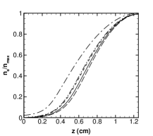
(a)

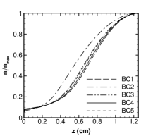
(b)

Figure 6: Spatial variation of (a) normalized electron number density and (b) normalized ion number density.

The maximum bulk plasma density, which is at the middle of the domain, is tabulated for various BCs in Table 3. To examine the effect of the BC on the sheath, the electron and ion number densities were normalized by the maximum plasma density with the results shown in Fig. 6. BC1 produces the largest sheath as a result of neglecting the flux to the boundary. While the sheath widths for BC1 and BC4 only vary by 3%, the difference is 10% in the bulk plasma density. BC2 produces the smallest sheath width and is the case where the normalized electron number density at the boundary is more pronounced than the other cases. This behavior is associated with a bulk density almost 200% higher than that in other cases. Neglecting the diffusion flux caused BC3 to have a smaller sheath than BC4 and a 26% higher bulk density. Inclusion of SEE does not suggest a significant impact on the sheath width.

V.3 Two-dimensional axisymmetric cylindrical configuration results

A cylindrical plasma reactor was modeled to investigate the influence of the different number and energy density BCs in an axisymmetric two-dimensional plasma. The plasma in this configuration is enclosed between two electrodes at the top and bottom of the domain and a dielectric lateral wall. Two groups of cases were modeled. In the first group, which was for the investigation of the electrode BC impact, the BC on the dielectric wall was identical (BC4, see Tab 2) among the cases while the number and energy density BC applied to the electrodes was different (BC1–5, see Tab 2). In the second group, which was for the investigation of the lateral BC impact, the electrode BC was identical (BC4, see Tab 2) among the cases while the number and energy density BC applied to the dielectric wall was different (BC1–5, see Tab 2).

V.3.1 Impact of the electrode boundary condition

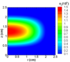
(a)

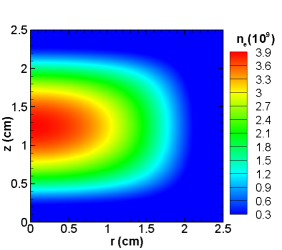
(b)

Figure 7: Contourplots of RF period-averaged electron number density (in 10⁹ cm^-3) with (a) BC1; and (b) BC2 as the electrode boundary condition. The lateral dielectric wall located at $r=2.5$ is set to BC4 in both subfigures.

Here, the axisymmetric cylindrical plasma reactor was modeled using the different sets of BCs, shown in Table 2, for the electrodes but the dielectric wall was set to BC4 in all cases. All BC kinds produced qualitatively similar results, with BC1 producing the lowest plasma density and BC2 producing the highest in the bulk of plasma. The RF-averaged electron number density contours are shown in Fig. 7 for BC1 and BC2.

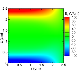
(a)

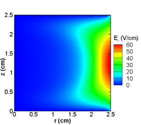
(b)

Figure 8: Contour plots of RF period-averaged electric field in V/cm, BC4 is used for both the electrodes and the lateral wall; (a) vertical electric field and (b) radial electric field.

To determine whether the ion extrapolation BC can be used, it is necessary to check the electric field along the boundary since ion extrapolation is only valid when the ions are flowing towards the boundary. An examination of the electric field, shown in Fig. 8 reveals that it is positive on the upper electrode and the wall, and negative on the lower electrode. However, the electric field magnitude near the corners is low. An examination of the time variation showed that there are times in the RF cycle where the electric field in the corners of the domain changes direction. Therefore, the ion extrapolation boundary condition cannot be applied for every point on the boundaries and it is necessary to check the local value of the electric field before using ion extrapolation. Applying an ion extrapolation BC did not have a significant effect on the plasma, compared to the base case.

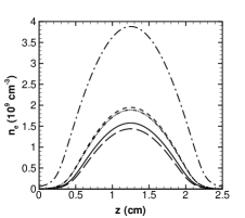
(a)

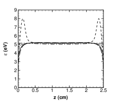
(b)

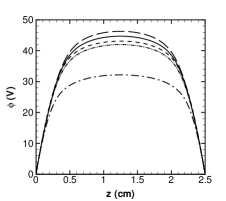
(c)

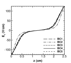
(d)

Figure 9: Spatial variation of RF-averaged plasma variables in the vertical direction at $r=0$ cm for the different electrode boundary conditions: (a) electron number density (in $10^{9}$ cm^-3); (b) mean electron energy (in eV); (c) electric potential (in V); and (d) vertical electric field (in V/cm).

The spatial variation of the RF-averaged plasma variable along the axisymmetric line ($r=0$) is plotted in Fig. 9. As seen in Fig. 9(a), BC2 has a substantially higher plasma density than the other cases, which is due to a lower rate of electron loss at the surface in this case. BC2 also produces a lower electric potential than the other cases, as seen in Fig. 9(c). The SEE, which is included in BC5, caused a 24% increase in the plasma density (Fig. 9(a)) and also caused a spike in the mean energy near the electrodes (Fig. 9(b)), compared to the base case.

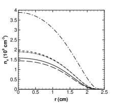
(a)

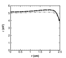
(b)

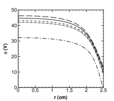
(c)

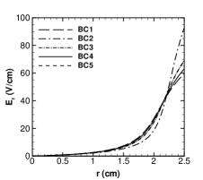
(d)

Figure 10: Spatial variation of RF-averaged plasma variables in the radial direction at $z=1.25$ cm, for the different electrode boundary conditions: (a) electron number density (in $10^{9}$ cm^-3); (b) mean electron energy (in eV); (c) electric potential (in V); and (d) radial electric field (in V/cm).

The radial variation of the plasma variables at $z=1.25$cm is plotted in Fig. 10. Since the dielectric wall BC was kept constant and did not include secondary emission, BC5 did not produce a spike in the mean energy near the wall, only near the electrodes. Also, since the electrode BC affected the bulk plasma density, it also affected the flux to the dielectric wall. Therefore, the electric field at the wall was affected by the choice of electrode BC. The magnitude of the electric field at the wall, as seen in Fig. 10(d), was lowest for BC1, which had the lowest plasma density, and highest for BC2, which had the highest plasma density.

The bulk plasma density calculated at the center of the reactor $z=1.25$ cm and $r=0$ cm, is given in Table 4 for the various cases. At the center, the RF-averaged densities are maximum, compared to the rest of the domain. It is seen in this table that the zero number density BC1 reduced the maximum plasma density by 9% compared to the baseline case, due to the larger sheath that occurs in BC1. BC3 had a 20% higher maximum plasma density than BC4 because diffusion flux to the surface is lacking in BC3. Secondary emission was of the same order as the diffusion flux with a 24% higher maximum plasma density for BC5 compared to BC4.

V.3.2 Impact of the dielectric wall boundary condition

Here, BC4 was used for electrodes and different BCs (Tab. 2) were used for the dielectric wall.

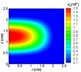
(a)

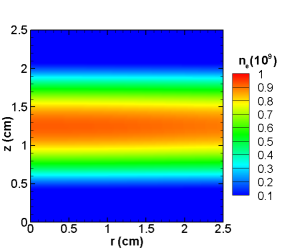
(b)

Figure 11: Contour plots of RF period-averaged electron number density (in 10⁹ cm^-3) for a dielectric wall (right boundary) using (a) BC1 and (b) BC2. The results produced by BC3, BC4, and BC5 were similar to BC1.

All cases, except the one using BC2 on the dielectric wall, produced similar results with the bulk plasma density varying less then 2% among the cases (Tab. 5). As seen in Fig. 11, BC2, which is the pure drift BC, did not produce a sheath at the wall, although there is a slight reduction in the density at the wall. The lack of sheath in the BC2 case for the dielectric wall, is a result of setting the electron flux to zero when the electric field is either zero or directed out of the domain. When this BC was applied to the electrodes, it caused an increase in the electron number density in the sheath and a reduction in the sheath width. This behavior is correlated with the strength of the electric field. A weaker field results in an even smaller sheath. For a dielectric wall, the electric field depends on the number density through the development of a wall charge, determined by eq. (10). When BC2 is used for ${\bm{\Gamma}}_{e}\cdot{\bm{n}}$, it prevents the development of a wall charge. This results in zero electric field, zero electron flux and zero wall charge. Setting the electric field and the fluxes to zero prevents the development of a sheath. Therefore, there is no sheath along the majority of the wall for BC2. The interaction between the electrodes and the wall near the corners of the domain causes the radial electric field in the corners of the domain to be non-zero which prevents a pure one-dimensional plasma.

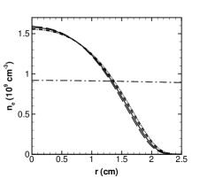
(a)

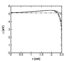
(b)

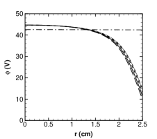
(c)

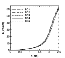
(d)

Figure 12: Spatial variation of RF-averaged plasma variables in the radial direction at z=1.25 cm, for the different wall boundary conditions: (a) electron number density (in $10^{9}$ cm^-3); (b) mean electron energy (in eV); (c) electric potential (in V); and (d) radial electric field (in V/cm).

The plasma variables are plotted against $r$ at $z=1.25$ cm in Fig. 12. The lack of a sheath on the dielectric wall when using BC2, is evident in all variables. BC3, which includes the thermal flux but neglects the diffusive flux, produced a higher electron mean energy at the wall; however, that is the only significant difference between BC3-5 and BC1. The effect of the SEE from the dielectric wall is not significant in this setup. BC5 shows a 1% decrease in the bulk plasma density, compared to BC4. The electric field at the dielectric wall is a function of the ion and electron flux to the wall, which suggests that the change of the number density BC should have a significant effect on the electric field. However, Fig. 12(d) shows that all the BCs except BC2 produce a RF-averaged radial electric field of 60 64 V/cm at the boundary. The use of BC2 results in zero radial electric field throughout the domain as evident in 11(b). This indicates that while the different BCs results in different values for the electron and ion fluxes at the wall, the increase or decrease in the electron flux is balanced out by a similar increase or decrease in the ion flux with the exception of BC2. Hence, the total current to the wall is similar for all BCs except BC2.

VI Conclusions

The change of the BC kinds implemented for the electrodes had a significant impact on the plasma. For the ions, the mobility was larger than the diffusion which caused the ions to be dominated by the drift motion. Therefore, since the electric field in an RF plasma generally causes the ions to flow out of the domain, the ion BC should not have a significant effect on the plasma. This was verified by the fact that using an ion extrapolation BC did not have a significant effect on the plasma.

The electrons have a larger diffusion and are not dominated by the drift motion in the same fashion as the ions. This behavior means the electron BC should have a significant effect and it is important to account for all the contributions to the electron flux at the boundary. Neglecting the flux and using the zero number density BC produces a 10% lower bulk plasma density than when the BC is based on a complete description of the flux to the electrode. Neglecting the thermal and diffusion fluxes and including only the drift towards the surface increases the bulk plasma density by a factor between two and three, compared to all the other BC’s. Including both the drift and the thermal fluxes but neglecting the diffusion flux resulted in a 20-30% increase in the bulk plasma density. Including secondary electron emission, with a coefficient of $\gamma=0.5$, resulted in a 20-25% increase in the bulk plasma density as a result of the increased mean energy in the sheath.

The plasma was less sensitive to the change of the dielectric wall BC than the electrode BC with the exception of the case where the electron BC at the wall was based on only the drift flux. The pure drift BC for the electrons failed to produce a sheath at the dielectric wall; hence, this BC is not recommended for the dielectric wall. The remaining BC’s for the dielectric wall produced bulk plasma densities within 2% of each other.

Appendix A Derivation of SEE BC

Substituting for $\bm{\Gamma}_{\alpha}\cdot\bm{n}$ and $\bm{\Gamma}_{\gamma}\cdot\bm{n}$ from eqs. (22) and (23), respectively, into $\bm{\Gamma}_{e}\cdot\bm{n}=\bm{\Gamma}_{\gamma}\cdot\bm{n}+\bm{\Gamma}_{\alpha}\cdot\bm{n}$ and using $n_{\alpha}=n_{e}-n_{\gamma}$, one obtains:

$$\bm{\Gamma}_{e}\cdot\bm{n}=\left[-\left(2a_{e}-1\right)\mu_{e}\bm{E}\cdot\bm{n}+\frac{1}{2}v_{\text{th}}\right]\left(n_{e}-n_{\gamma}\right)-\left(1-a_{e}\right)\gamma\bm{\Gamma}_{i}\cdot\bm{n}.$$ (36)

Expanding the first term and substituting for $n_{\gamma}$ from eq. (24) in the drift term gives:

$$\begin{gathered}\bm{\Gamma}_{e}\cdot\bm{n}=\left[-\left(2a_{e}-1\right)\mu_{e}\bm{E}\cdot\bm{n}+\frac{1}{2}v_{\text{th}}\right]n_{e}-\frac{1}{2}v_{\text{th}}n_{\gamma}\\ +\left(2a_{e}-1\right)\left[\left(1-a_{e}\right)\frac{\gamma\bm{\Gamma}_{i}\cdot\bm{n}}{\mu_{e}\bm{E}\cdot\bm{n}}\right]\mu_{e}\bm{E}\cdot\bm{n}-\left(1-a_{e}\right)\gamma\bm{\Gamma}_{i}\cdot\bm{n},\end{gathered}$$ (37)

which simplifies to the following equation after factoring out $(1-a_{e})$ between the last two terms:

$$\begin{gathered}\bm{\Gamma}_{e}\cdot\bm{n}=\left[-\left(2a_{e}-1\right)\mu_{e}\bm{E}\cdot\bm{n}+\frac{1}{2}v_{\text{th}}\right]n_{e}-\frac{1}{2}v_{\text{th}}n_{\gamma}\\ -2\left(1-a_{e}\right)^{2}\gamma\bm{\Gamma}_{i}\cdot\bm{n}.\end{gathered}$$ (38)

Using the definition of $a_{e}$ given in eq. (12), it can be shown that $\left(1-a_{e}\right)^{2}=\left(1-a_{e}\right)$, so the BC for the electrons in eq. (25) is derived. The equation for the energy density given in eq. (29) is derived in a similar fashion.

References

Table 1: Plasma parameters

Parameter	Value
Electrode gap, H	2.5 (cm)
Electrode radius, R	2.5 (cm)
Applied voltage, $V_{\text{RF}}$	50 (V)
Frequency, $f$	13.56 (MHz)
Neutral gas pressure, $P_{\text{gas}}$	250 (mTorr)
Ion and neutral temperature, $T_{i}=T_{\text{gas}}$	300 (K)
Electron mobility $\mu_{e}P_{gas}$	3$\times$105
Electron diffusion $D_{e}P_{gas}$	1.2$\times$106
Ion mobility $\mu_{i}P_{gas}$	1400
Ion diffusion $D_{i}P_{gas}$	40

Table 2: Number and energy density boundary conditions

Label	Description	Equations
BC1	Zero number density (Sec. III.2.1)	—
BC2	Pure drift towards the electrode (Sec. III.2.2)	(13,14)
BC3	Thermal flux (Sec. III.2.3)	(15,17)
BC4 (baseline)	Thermal and diffusion fluxes (Sec. III.2.4)	(19,21)
BC5	Secondary emission with $\gamma=0.5$ (Sec. III.2.5)	(19,25,29)

Table 3: Effect of boundary conditions on maximum bulk plasma density in the one dimensional plasma.

Boundary	Bulk plasma	% difference
condition	maximum density (cm-3)	(vs BC4)
BC1	8.32$\times$108	-10.8%
BC2	2.75$\times$109	195%
BC3	1.18$\times$109	26.1%
BC4 (baseline)	9.34$\times$108	N/A
BC5	1.15$\times$109	22.6%

Table 4: Effect of boundary conditions on maximum bulk plasma density for the axisymmetric plasma; the lateral wall used BC4 and the electrode boundary condition was varied.

Boundary	Bulk plasma	% difference
condition	density (cm-3)	(vs BC4)
BC1	1.45$\times$109	-8.7%
BC2	3.89$\times$109	145.3%
BC3	1.90$\times$109	19.6%
BC4 (baseline)	1.58$\times$109	N/A
BC5	1.96$\times$109	23.5%

Table 5: Effect of boundary conditions on maximum bulk plasma density for the axisymmetric plasma; the electrodes used BC4 and the wall boundary condition was varied.

Boundary	Bulk plasma	% difference
condition	density (cm-3)	(vs BC4)
BC1	1.60$\times$109	0.8%
BC2	9.27$\times$108	-41.5%
BC3	1.56$\times$109	-1.5%
BC4 (baseline)	1.58$\times$109	N/A
BC5	1.57$\times$109	-0.9%

References

- (1) A. Stoffel, A. Kovacs, W. Kronast, B. Müller, LPCVD against PECVD for micromechanical applications, Journal of Micromechanics and Microengineering 6 (1) (1996) 1.
- (2) X. Michalet, F. Pinaud, L. Bentolila, J. Tsay, S. Doose, J. Li, G. Sundaresan, A. Wu, S. Gambhir, S. Weiss, Quantum dots for live cells, in vivo imaging, and diagnostics, Science 307 (5709) (2005) 538–544.
- (3) X. Pi, R. Liptak, J. D. Nowak, N. Wells, C. Carter, S. Campbell, U. Kortshagen, Air-stable full-visible-spectrum emission from silicon nanocrystals synthesized by an all-gas-phase plasma approach, Nanotechnology 19 (24) (2008) 245603.
- (4) J. Cao, T. Matsoukas, Deposition kinetics on particles in a dusty plasma reactor, Journal of Applied Physics 92 (5) (2002) 2916–2922.
- (5) M. Meyyappan, L. Delzeit, A. Cassell, D. Hash, Carbon nanotube growth by PECVD: A review, Plasma Sources Science and Technology 12 (2) (2003) 205.
- (6) P. Shukla, A survey of dusty plasma physics, Physics of Plasmas (1994-present) 8 (5) (2001) 1791–1803.
- (7) H. Ikezi, Coulomb solid of small particles in plasmas, Physics of Fluids (1958-1988) 29 (6) (1986) 1764–1766.
- (8) V. Schweigert, I. Schweigert, A. Melzer, A. Homann, A. Piel, Alignment and instability of dust crystals in plasmas, Physical Review E 54 (4) (1996) 4155.
- (9) L. S. Matthews, V. Land, T. W. Hyde, Charging and coagulation of dust in protoplanetary plasma environments, The Astrophysical Journal 744 (1) (2011) 8.
- (10) O. Havnes, T. K. Aanesen, F. Melandsø, On dust charges and plasma potentials in a dusty plasma with dust size distribution, Journal of Geophysical Research: Space Physics 95 (A5) (1990) 6581–6585.
- (11) M. Moisan, J. Barbeau, S. Moreau, J. Pelletier, M. Tabrizian, L. Yahia, Low-temperature sterilization using gas plasmas: a review of the experiments and an analysis of the inactivation mechanisms, International Journal of Pharmaceutics 226 (1) (2001) 1–21.
- (12) M. Laroussi, Low temperature plasma-based sterilization: Overview and state-of-the-art, Plasma Processes and Polymers 2 (5) (2005) 391–400.
- (13) G. Fridman, G. Friedman, A. Gutsol, A. B. Shekhter, V. N. Vasilets, A. Fridman, Applied plasma medicine, Plasma Processes and Polymers 5 (6) (2008) 503–533.
- (14) J. Schlegel, J. Köritzer, V. Boxhammer, Plasma in cancer treatment, Clinical Plasma Medicine 1 (2) (2013) 2–7.
- (15) S.-K. Park, D. J. Economou, Analysis of low pressure rf glow discharges using a continuum model, Journal of Applied Physics 68 (8) (1990) 3904–3915.
- (16) W. Goedheer, M. Akdim, Y. I. Chutov, Hydrodynamic and kinetic modelling of dust free and dusty radio-frequency discharges, Contributions to Plasma Physics 44 (5-6) (2004) 395–404.
- (17) B. Parent, S. O. Macheret, M. N. Shneider, Electron and ion transport equations in computational weakly-ionized plasmadynamics, Journal of Computational Physics 259 (2014) 51–69.
- (18) M. Zakari, H. Caquineau, P. Hotmar, P. Segur, An axisymmetric unstructured finite volume method applied to the numerical modeling of an atmospheric pressure gas discharge, Journal of Computational Physics 281 (2015) 473–492.
- (19) M. S. Barnes, T. J. Cotler, M. E. Elta, Large-signal time-domain modeling of low-pressure rf glow discharges, Journal of Applied Physics 61 (1) (1987) 81–89.
- (20) G. Grubert, M. Becker, D. Loffhagen, Why the local-mean-energy approximation should be used in hydrodynamic plasma descriptions instead of the local-field approximation, Physical Review E 80 (3) (2009) 036405.
- (21) D. B. Graves, K. F. Jensen, A continuum model of dc and rf discharges, IEEE Transactions on Plasma Science 14 (2) (1986) 78–91.
- (22) E. Gogolides, H. H. Sawin, Continuum modeling of radio-frequency glow discharges. i. theory and results for electropositive and electronegative gases, Journal of Applied Physics 72 (9) (1992) 3971–3987.
- (23) E. Hammond, K. Mahesh, P. Moin, A numerical method to simulate radio-frequency plasma discharges, Journal of Computational Physics 176 (2) (2002) 402–429.
- (24) G. Hagelaar, F. De Hoog, G. Kroesen, Boundary conditions in fluid models of gas discharges, Physical Review E 62 (1) (2000) 1452.
- (25) S. T. Surzhikov, J. S. Shang, Two-component plasma model for two-dimensional glow discharge in magnetic field, Journal of Computational Physics 199 (2) (2004) 437–464.
- (26) F. Bouanaka, S. Rebiai, Effect of secondary electron emission on argon glow discharge characteristics, Detection of Absolute Rest Frame by Measuring Light Wavelength of Light Source in Uniform Rectilinear Motion (2013) 81.
- (27) J. Boeuf, L. Pitchford, Two-dimensional model of a capacitively coupled rf discharge and comparisons with experiments in the gaseous electronics conference reference reactor, Physical Review E 51 (2) (1995) 1376.
- (28) M. Davoudabadi, F. Mashayek, Numerical modeling of dust particle configurations in a cylindrical radio-frequency plasma reactor, Physical Review E 76 (5) (2007) 056405.
- (29) J. Passchier, W. Goedheer, A two-dimensional fluid model for an argon rf discharge, Journal of Applied Physics 74 (6) (1993) 3744–3751.
- (30) M. Davoudabadi, J. S. Shrimpton, F. Mashayek, On accuracy and performance of high-order finite volume methods in local mean energy model of non-thermal plasmas, Journal of Computational Physics 228 (7) (2009) 2468–2479.
- (31) C. Horn, M. Davoudabadi, B. Shotorban, Effects of radiofrequency on dust particle dynamics in a plasma reactor, Journal of Applied Physics 110 (11) (2011) 113305.
- (32) T. Paunska, A. Shivarova, K. Tarnev, Comments on the boundary conditions for metal and dielectric walls in the fluid-plasma modelling, 30th ICPIG.
- (33) G. Gozadinos, A. Ivlev, J. Boeuf, A fluid model for colloidal plasmas under microgravity conditions, New Journal of Physics 5 (1) (2003) 32.
- (34) G. Hagelaar, L. Pitchford, Solving the boltzmann equation to obtain electron transport coefficients and rate coefficients for fluid models, Plasma Sources Science and Technology 14 (4) (2005) 722.
- (35) V. Land, E. Shen, B. Smith, L. Matthews, T. Hyde, Experimental and computational characterization of a modified gec cell for dusty plasma experiments, New Journal of Physics 11 (6) (2009) 063024.
- (36) M. Surendra, D. Graves, G. Jellum, Self-consistent model of a direct-current glow discharge: Treatment of fast electrons, Physical Review A 41 (2) (1990) 1112.
- (37) T. Nitschke, D. Graves, A comparison of particle in cell and fluid model simulations of low-pressure radio frequency discharges, Journal of Applied Physics 76 (10) (1994) 5646–5660.
- (38) E. A. Bogdanov, A. A. Kudryavtsev, Z. S. Ochikova, Main scenarios of spatial distribution of charged and neutral components in plasma, IEEE Transactions on Plasma Science 41 (12) (2013) 3254–3267.
- (39) I. Rafatov, E. Bogdanov, A. Kudryavtsev, Account of nonlocal ionization by fast electrons in the fluid models of a direct current glow discharge, Physics of Plasmas 19 (9) (2012) 093503.
- (40) S. Wen-Xia, P. Qing-Jun, Y. Qing, Y. Tao, S. Jian, Local electron mean energy profile of positive primary streamer discharge with pin-plate electrodes in oxygen—nitrogen mixtures, Chinese Physics B 22 (1) (2013) 015203.
- (41) L. Liu, D. Mihailova, J. Van Dijk, J. ten Thije Boonkkamp, Efficient simulation of drift–diffusive discharges: application of the ‘complete flux scheme’, Plasma Sources Science and Technology 23 (1) (2014) 015023.
- (42) H.-J. Lee, S. Park, J. Eden, Pulsed microplasmas generated in truncated paraboloidal microcavities: simulations of particle densities and energy flow, Journal of Physics D: Applied Physics 45 (40) (2012) 405201.
- (43) M. Iqbal, M. Turner, Spatial uniformity of atmospheric pressure discharges: A simulation study, Contributions to Plasma Physics 54 (9) (2014) 756–771.
- (44) M. Becker, T. Hoder, R. Brandenburg, D. Loffhagen, Analysis of microdischarges in asymmetric dielectric barrier discharges in argon, Journal of Physics D: Applied Physics 46 (35) (2013) 355203.
- (45) D. L. Scharfetter, H. K. Gummel, Large-signal analysis of a silicon read diode oscillator, IEEE Transactions on Electron Devices 16 (1) (1969) 64–77.
- (46) J.-P. Boeuf, Numerical model of rf glow discharges, Physical Review A 36 (6) (1987) 2782.
- (47) G. Hagelaar, G. Kroesen, Speeding up fluid models for gas discharges by implicit treatment of the electron energy source term, Journal of Computational Physics 159 (1) (2000) 1–12.
- (48) M. M. Becker, H. Kählert, A. Sun, M. Bonitz, D. Loffhagen, Advanced fluid modeling and pic/mcc simulations of low-pressure ccrf discharges, Plasma Sources Science and Technology 26 (4) (2017) 044001.