QuickMergesort: Practically Efficient Constant-Factor Optimal Sorting

Abstract.

We consider the fundamental problem of internally sorting a sequence of $n$ elements. In its best theoretical setting QuickMergesort, a combination Quicksort with Mergesort with a Median-of-$\sqrt{n}$ pivot selection, requires at most $n\log n-1.3999n+o(n)$ element comparisons on the average. The questions addressed in this paper is how to make this algorithm practical. As refined pivot selection usually adds much overhead, we show that the Median-of-3 pivot selection of QuickMergesort leads to at most $n\log n-0{.}75n+o(n)$ element comparisons on average, while running fast on elementary data. The experiments show that QuickMergesort outperforms state-of-the-art library implementations, including C++’s Introsort and Java’s Dual-Pivot Quicksort. Further trade-offs between a low running time and a low number of comparisons are studied. Moreover, we describe a practically efficient version with $n\log n+\mathcal{O}(n)$ comparisons in the worst case.

1. Introduction

Sorting a sequence of $n$ elements remains one of the most fascinating topics in computer science, and runtime improvements to sorting has significant impact for many applications. The lower bound is $\log(n!)\approx n\log n-1.44n+\Theta(\log n)$ element comparisons applies to the worst and the average case.

The sorting algorithms we propose in this paper are internal or in-place: they need at most $\mathcal{O}(\log n)$ space (computer words) in addition to the array to be sorted. That means we consider Quicksort [15] an internal algorithm, whereas standard Mergesort is external because it needs a linear amount of extra space.

Based on QuickHeapsort [5, 7], Edelkamp and Weiß [9] developed the concept of QuickXsort and applied it to X = WeakHeapsort [8] and X = Mergesort. The idea – going back to UltimateHeapsort [17] – is very simple: as in Quicksort the array is partitioned into the elements greater and less than some pivot element, respectively. Then one part of the array is sorted by X and the other part is sorted recursively. The advantage is that, if X is an external algorithm, then in QuickXsort the part of the array which is not currently being sorted may be used as temporary space, which yields an internal variant of X.

Using Mergesort as X, a partitioning scheme with $\lceil\sqrt{n}\rceil$ pivots, known to be optimal for classical Quicksort [22], and Ford and Johnson’s MergeInsertion as the base case [13], QuickMergesort requires at most $n\log n-1.3999n+o(n)$ element comparisons on the average (and $n\log n-1.4n+o(n)$ for $n=2^{k}$), while preserving worst-case bounds $n\log n+\mathcal{O}(n)$ element comparisons and $\mathcal{O}(n\log n)$ time for all other operations [9]. To the authors’ knowledge the average-case result is the best-known upper bound for sequential sorting with $\mathcal{O}(n\log n)$ overall time bound, in the leading term matching, and in the linear term being less than $0.045n$ away from the lower bound. The research question addressed in this paper, is whether QuickMergesort can be made practical in relation to efficient library implementations for sorting, such as Introsort and Dual-Pivot Quicksort.

Introsort [23], implemented as std::sort in C++/STL, is a mix of Insertionsort, CleverQuicksort (the Median-of-3 variant of Quicksort) and Heapsort [12, 28], where the former and latter are used as recursion stoppers (the one for improving the performance for small sets of data, the other one for improving worst-case performance). The average-time complexity, however, is dominated by CleverQuicksort.

Dual-Pivot Quicksort by Yaroslavskiy et al. as implemented in current versions of Java (e.g., Oracle Java 7 and Java 8) is an interesting Quicksort variant using two (instead of one) pivot elements in the partitioning stage (recent proposals use three and more pivots [20]). It has been shown that – in contrast to ordinary Quicksort with an average case of $2\cdot n\ln n+\mathcal{O}(n)$ element comparisons – Dual-Pivot Quicksort requires at most $1.9\cdot n\ln n+\mathcal{O}(n)$ element comparisons on the average, and there are variants that give $1.8\cdot n\ln n+\mathcal{O}(n)$. For a rising number of samples for pivot selection, the leading factor decreases [2, 27, 3].

So far there is no practical (competitive in performance to state-of-the-art library implementations) sorting algorithm that is internal and constant-factor-optimal (optimal in the leading term). Maybe closest is InSituMergesort [18, 11], but even though that algorithm improves greatly over the library implementation of in-place stable sort in STL, it could not match with other internal sorting algorithms. Hence, the aim of the paper is to design fast QuickMergesort variants. Instead of using a Median-of-$\sqrt{n}$ strategy, we will use the Median-of-3. For Quicksort, the Median-of-3 strategy is also known as CleverQuicksort. The leading constant in $c\cdot n\log n+\mathcal{O}(n)$ for the average case of comparisons of CleverQuicksort is $c=(12/7)\ln 2\approx 1.188$. As $c<1.8\ln 2$, CleverQuicksort is theoretically superior to the wider class of DualPivotQuicksort algorithms considered in [2, 3, 27].

Another sorting algorithm studied in this paper is a mix of QuickMergesort and CleverQuicksort: during the sorting with Mergesort, for small arrays CleverQuicksort is applied.

The contributions of the paper are as follows.

1. We derive a bound on the average number of comparisons in QuickMergesort when the Median-of-3 partitioning strategy is used instead of the Median-of-$\sqrt{n}$ strategy, and show a surprisingly low upper bound of $n\log n-0.75n+o(n)$ comparisons on average.

2. We analyze a variant of QuickMergesort where base cases of size at most $n^{\beta}$ for some $\beta\in[0,1]$ are sorted using yet another sorting algorithm X; otherwise the algorithm is identical to QuickMergesort. We show that if X is called for about $\sqrt{n}$ elements and X uses at most $\alpha\cdot n\log n+\mathcal{O}(n)$ comparisons on average, the average number of comparisons of is $(1+\alpha)/2\cdot n\log n+\mathcal{O}(n)$, with $(1+\alpha)/2\approx 1.094$ for X $=$ Median-of-3 Quicksort. Other element size thresholds for invoking X lead to further trade-offs.

3. We refine a trick suggested in [9] in order to obtain a bound of $n\log n+16.1n$ comparisons in the worst case using the median-of-median algorithm [4] with an adaptive pivot sampling strategy. On average the modified algorithm is only slightly slower than the Median-of-3 variant of QuickMergesort.

4. We compare the proposals empirically to other algorithms from the literature.

We start with revisiting QuickXsort and especially QuickMergesort, including theoretically important and practically relevant sub-cases. We derive an upper bound on the average number of comparisons in QuickMergesort with Median-of-3 pivot selection. In Section 3, we present changes to the algorithm that lead to the hybrid QuickMergeXsort. Next, we introduce the worst-case efficient variant MoMQuickMergesort, and, finally, we present experimental results.

2. QuickXsort and QuickMergesort

In this section we give a brief description of QuickXsort and extend a result concerning the number of comparisons performed in the average case.

Let X be some sorting algorithm. QuickXsort works as follows: First, choose a pivot element as the median of some sample (the performance will depend on the size of the sample). Next, partition the array according to this pivot element, i. e., rearrange the array such that all elements left of the pivot are less or equal and all elements on the right are greater or equal than the pivot element. Then, choose one part of the array and sort it with the algorithm X. After that, sort the other part of the array recursively with QuickXsort.

The main advantage of this procedure is that the part of the array that is not being sorted currently can be used as temporary memory for the algorithm X. This yields fast internal variants for various external sorting algorithms such as Mergesort. The idea is that whenever a data element should be moved to the extra (additional or external) element space, instead it is swapped with the data element occupying the respective position in part of the array which is used as temporary memory. Of course, this works only if the algorithm needs additional storage only for data elements. Furthermore, the algorithm has to keep track of the positions of elements which have been swapped.

For the number of comparisons some general results hold for a wide class of algorithms X. Under natural assumptions the average number of comparisons of X and of QuickXsort differ only by an $o(n)$-term: Let X be some sorting algorithm requiring at most $n\log n+cn+o(n)$ comparisons on average. Then, QuickXsort with a Median-of-$\sqrt{n}$ pivot selection also needs at most $n\log n+cn+o(n)$ comparisons on average [9]. Sample sizes of approximately $\sqrt{n}$ are likely to be optimal [7, 22].

If the unlikely case happens that always the $\sqrt{n}$ smallest elements are chosen for pivot selection, $\Omega(n^{3/2})$ comparisons are performed. However, as we showed in [9], such a worst case is unlikely. Nevertheless, for improving the worst-case complexity, in [9] we suggested a trick similar to Introsort [23] leading to $n\log n+\mathcal{O}(n)$ comparisons in the worst case (use the median of the whole array as pivot if the previous pivot was very bad). In Section 4 of this paper, we refine this method yielding a better average and worst-case performance.

One example for QuickXsort is QuickMergesort. For the Mergesort part we use standard (top-down) Mergesort, which can be implemented using $m$ extra element spaces to merge two arrays of length $m$. After the partitioning, one part of the array – for a simpler description we assume the first part – has to be sorted with Mergesort (note, however, that any of the two sides can be sorted with Mergesort as long as the other side contains at least $n/3$ elements. In order to do so, the second half of this first part is sorted recursively with Mergesort while moving the elements to the back of the whole array. The elements from the back of the array are inserted as dummy elements into the first part. Then, the first half of the first part is sorted recursively with Mergesort while being moved to the position of the former second half of the first part. Now, at the front of the array, there is enough space (filled with dummy elements) such that the two halves can be merged. The executed stages of the algorithm QuickMergesort (with no median pivot selection strategy applied) are illustrated in Fig 1.

partitioning leads to

Figure 1. Example for the execution of QuickMergesort.

Mergesort requires approximately $n\log n-1.26n$ comparisons on average, so that with a Median-of-$\sqrt{n}$ we obtain an internal sorting algorithm with $n\log n-1.26n+o(n)$ comparisons on average. One can do even better by sorting small subarrays with a more complicated algorithm requiring less comparisons – for details see [9].

Since the Median-of-3 variant (i. e. CleverQuickMergesortsort) shows a slightly better practical performance than with Median-of-$\sqrt{n}$ (see [9]), we provide here a theoretical analysis of it by showing that CleverQuickMergesortsort performs at most $n\log n-0.75n+o(n)$ comparisons on average. In fact, as in [9] we show a more general result for CleverQuickXsort for an arbitrary algorithm X.

Theorem 2.1 (Average Case CleverQuickXsort).

Let the algorithm X perform at most $\alpha n\log n+cn+\mathcal{O}(\log n)$ comparisons on average. Then, CleverQuickXsort performs at most $\alpha n\log n+(c+\kappa_{\alpha})n+\mathcal{O}(\log^{2}n)$ comparisons on average with $\kappa_{\alpha}=\frac{4}{15}\left(12-\frac{7\alpha}{\ln 2}\right)\leq 0{.}51$.

Since Mergesort requires at most $n\log n-1.26n+o(n)$ comparisons on average, we obtain the following corollary:

Corollary 2.2 (Average Case CleverQuickMergesort).

CleverQuickMergesort is an in-place algorithm that performs at most $n\log n-0.75n+o(n)$ comparisons on average.

Proof 2.3 (Proof of Theorem 2.1).

The probability of choosing the $k$-th element (in the ordered sequence) as pivot of a random $n$-element array is $\mathop{\mathrm{Pr}}\left[\,\!\text{pivot }=k\!\,\right]=(k-1)(n-k){\binom{n}{3}}^{-1}$ (one element of the three element set has to be less than the $k$-th, one equal to the $k$-th, and one greater than $k$-th element of the array). Note that this holds no matter whether we select the three elements at random or we use fixed positions and average over all input permutations. Since probabilities sum up to 1, we have

$$\sum_{k=1}^{n}(k-1)(n-k){\binom{n}{3}}^{-1}=1.$$ (1)

Moreover, partitioning preserves randomness of the two sides of the array – this includes the positions where the other two elements from the pivot sample are placed (since for a fixed pivot, every element smaller (resp. greater) than the pivot has the same probability of being part of the sample). Also, using the array as temporary space for Mergesort does not destroy randomness since the dummy elements are never compared.

Let $T(n)$ be the average-case number of comparisons of CleverQuickXsort for sorting an input of size $n$ and let

$$S(n)=\alpha n\log n+cn+d(1+\log n)$$

be a bound for the average number of comparisons of the algorithm X (e. g. Mergesort). We will show by induction that

$$T(n)\leq\alpha n\log n+(c+\kappa_{\alpha})n+D(1+\log^{2}n)$$

for some constant $D\geq d$ (which we specify later such that the induction base is satisfied) and $\kappa_{\alpha}=\frac{4}{15}\left(12-\frac{7\alpha}{\ln 2}\right)\leq 0.51$ (since $\alpha\geq 1$ by the general lower bound on sorting). As induction hypothesis for $1\leq k\leq n$ we assume that

$$\max\{\,T(k-1) +S(n-k),T(n-k)+S(k-1)\,\}$$

$$\leq\alpha(k-1)\log(k-1)+\alpha(n-k)\log(n-k)+cn+\kappa_{\alpha}\max\{k-1,n-k\}$$

$$\qquad+D\left(1+\log^{2}(\max\{k-1,n-k\})\right)+d\left(1+\log(\min\{k-1,n-k\})\right)$$

$$=:f(n,k).$$

In order to find the pivot element, three comparisons are needed. After that, for partitioning $n-3$ comparisons are performed (all except the three elements of the pivot sample are compared with the pivot). Since after partitioning, one part of the array is sorted with X and the other recursively with CleverQuickXsort, we obtain the recurrence

$$T(n) \leq n+\sum_{k=1}^{n}\mathop{\mathrm{Pr}}\left[\,\!\text{pivot }=k\!\,\right]\cdot\max\left\{\,T(k-1)+S(n-k),T(n-k)+S(k-1)\,\right\}$$

$$\leq n+\sum_{k=1}^{n}\frac{(k-1)(n-k)}{\binom{n}{3}}f(n,k)$$

$$\leq n+\frac{1}{\binom{n}{3}}\sum_{k=1}^{n}(k-1)(n-k)\Bigl{(}\alpha(k-1)\log(k-1)+\alpha(n-k)\log(n-k)\Bigr{)}$$ (2)

$$\qquad+\frac{1}{\binom{n}{3}}\sum_{k=1}^{n}(k-1)(n-k)\kappa_{\alpha}\max\{k-1,n-k\}$$ (3)

$$\qquad+\frac{1}{\binom{n}{3}}\sum_{k=1}^{n}(k-1)(n-k)D\log^{2}(\max\{k-1,n-k\})$$ (4)

$$\qquad+\frac{1}{\binom{n}{3}}\sum_{k=1}^{n}(k-1)(n-k)\Bigl{(}cn+D+d+d\log\left(\min\{k-1,n-k\}\right)\Bigr{)}$$ (5)

We simplify the terms (2)–(5) separately using http://www.wolframalpha.com/ for evaluating the sums and integrals. The function $x\mapsto g(x)=(x-1)^{2}(n-x)\log(x-1)$ is non-negative and has a single maximum for $1\leq x\leq n$ at position $x=\xi$; on the left of $\xi$, it is monotonically increasing, on the right monotonically decreasing. Therefore,

$$\sum_{k=1}^{n}g(k) =\sum_{k=1}^{\left\lfloor\mathinner{\xi}\right\rfloor}g(k)+\sum_{k=\left\lfloor\mathinner{\xi}\right\rfloor+1}^{n}g(k)\ \leq\int_{1}^{\left\lfloor\mathinner{\xi}\right\rfloor}g(x)\,dx+\int_{\left\lfloor\mathinner{\xi}\right\rfloor+1}^{n}g(x)\,dx+2g(\xi).$$

Since the second term of (2) is obtained from the first one by a substitution $k\mapsto n+1-k$, it follows that

$$(\ref{eq:nlogn})-n \leq\frac{\alpha}{\binom{n}{3}}\cdot\Biggl{(}\int_{1}^{n}g(x)\,dx+\int_{1}^{n}g(n+1-x)\,dx+4g(\xi)\Biggr{)}$$

$$\leq\frac{\alpha}{\binom{n}{3}}\cdot\Biggl{(}2\int_{1}^{n}x^{2}(n-x)\log x\,dx+4n^{3}\log n\Biggr{)}$$

$$=\frac{\alpha}{\binom{n}{3}}\cdot\Biggl{(}\frac{2}{144\ln 2}n^{4}(12\ln n-7)+4n^{3}\log n\Biggr{)}\leq\alpha n\log n-\frac{7\alpha}{12\ln 2}n+c_{3}\alpha\log n$$

for some properly chosen constant $c_{3}$. Now, first assume that $\kappa_{\alpha}\geq 0$. Then we have

$$(\ref{eq:ckappa}) \leq\frac{2\kappa_{\alpha}}{\binom{n}{3}}\sum_{k=1}^{\left\lceil\mathinner{n/2}\right\rceil}(k-1)(n-k)^{2}\leq\frac{2\kappa_{\alpha}n}{192\binom{n}{3}}\left(11n^{3}-20n^{2}-44n+80\right)\leq\frac{11}{16}\kappa_{\alpha}n+c_{4}$$

for some constant $c_{4}$. On the other hand, if $\kappa_{\alpha}<0$, we have

$$(\ref{eq:ckappa}) \leq\frac{2\kappa_{\alpha}}{\binom{n}{3}}\sum_{k=1}^{\left\lfloor\mathinner{n/2}\right\rfloor}(k-1)(n-k)^{2}\leq\frac{2\kappa_{\alpha}n}{192\binom{n}{3}}\left(11n^{3}-68n^{2}-100n+16\right)\leq\frac{11}{16}\kappa_{\alpha}n+c_{4}$$

for some constant $c_{4}$. Thus, in any case, we have $(\ref{eq:ckappa})\leq\frac{11}{16}\kappa_{\alpha}n+c_{4}$. With the same argument as for (2), we have

$$(\ref{eq:logsquare}) \leq\frac{2D}{\binom{n}{3}}\sum_{k=\left\lfloor\mathinner{n/2}\right\rfloor}^{n}(k-1)(n-k)\log^{2}(k-1)$$

$$\leq\frac{2D}{\binom{n}{3}}\int_{\left\lfloor\mathinner{n/2}\right\rfloor}^{n}(x-1)(n-x)\log^{2}(x-1)\,dx+D\cdot c_{5}^{\prime}\leq D\log^{2}n-\frac{5D}{3}\log n+D\cdot c_{5}$$

for some constants $c_{5}^{\prime}$ and $c_{5}$. Finally, by (1), we have

$$(\ref{eq:rest})\leq cn+D+d+d\log(n/2)=cn+D+d\log n.$$

Now, we combine all the terms and obtain

$$T(n) \leq\alpha n\log n+n\left(1+\frac{-7\alpha}{12\ln 2}+c+\frac{11}{16}\kappa_{\alpha}\right)$$

$$\qquad+c_{3}\alpha\log n+c_{4}+D\log^{2}n-\frac{5D}{3}\log n+Dc_{5}+D+d\log n$$

We can choose $D$ such that $\frac{5D}{3}\log n\geq c_{3}\alpha\log n+c_{4}+Dc_{5}+D+d\log n$ for $n$ large enough and $D\geq T(n)$ for all smaller $n$. Hence, we conclude the proof of Theorem 2.1:

$$T(n) \leq\alpha n\log n+n\left(1+\frac{-7\alpha}{12\ln 2}+c+\frac{11}{16}\kappa_{\alpha}\right)+D\log^{2}n+D$$

$$=\alpha n\log n+n\left(1+\frac{-7\alpha}{12\ln 2}+c+\frac{11}{16}\cdot\frac{4}{15}\left(12-\frac{7\alpha}{\ln 2}\right)\right)+D\log^{2}n+D$$

$$=\alpha n\log n+(c+\kappa_{\alpha})n+D\log^{2}n+D.$$

Notice that in the case that in each recursion level always the smaller part is sorted with X, the inequalities in the proof of Theorem 2.1 are tight up to some lower order terms. Thus, the proof can be easily modified to provide a lower bound of $\alpha n\log n+(c+\kappa_{\alpha})n-\mathcal{O}(\log^{2}n)$ comparisons in this special case.

3. QuickMergeXsort

QuickMergeXsort agrees with QuickMergesort up to the following change: for arrays of size smaller than some threshold cardinality X_THRESH, the sorting algorithm X is called (instead of Mergesort) and the sorted elements are moved to their target location expected by QuickMergesort.

Fig. 2 provides the full implementation details of QuickMerge(X)sort (in C++). The realization of the sorting algorithm X and the partitioning algorithm have to be added. The listing shows that by dropping the base cases from QuickMergesort the code is short enough for textbooks on algorithms and data structures. The general principle is that we have a merging step that takes two sorted areas, merges and swaps them into a third one.

The program msort applies Mergesort with X as a stopper. It goes down the recursion tree and shrinks the size of the array accordingly. If the array is small enough, the algorithm calls X followed by a joint movement (memory copy) of array elements (the only change of code wrt. QuickMergesort). The algorithm out serves as an interface between the recursive procedure msort and top-level procedure sort. Last, but not least, we have the overall internal sorting algorithm sort, that performs the partitioning.

⬇

1 typedef std::vector<t>::iterator iter;

2 void merge(iter begin1, iter end1, iter target, iter endtarget) {

3 iter i1 = begin1, i2 = target + (end1 - begin1), ires = target;

4 t temp = *target;

5 while (i1 != end1 && i2 != endtarget) {

6 iter tempit = (*i1 < *i2) ? i1++ : i2++;

7 *ires++ = *tempit; *tempit = *ires;

8 }

9 while(i1 < end1) { *ires++ = *i1; *i1++ = *ires; }

10 *(i1 - 1) = temp;

11 }

12 void msort(iter begin, iter end, iter target) {

13 index n = end - begin;

14 if (n < X_THRESH) {

15 X(begin, end);

16 for(int i=0; i<n; i++) std::swap(begin[i], target[i])

17 }

18 else {

19 index q = n / 2;

20 msort(begin + q, end, target + q);

21 msort(begin, begin + q, begin + q);

22 merge(begin + q, begin + n , target, target + n);

23 }

24 }

25 void out(iter begin, iter end, iter temp) {

26 index n = end - begin;

27 if (n > 1) {

28 index q = n / 2, r = n - q;

29 msort(begin + q, end, temp);

30 msort(begin, begin + q, begin + r);

31 merge(temp , temp + r , begin, end);

32 }

33 }

34 void sort(std::vector<t> &a) {

35 iter begin = a.begin(), end = a.end();

36 while (begin < end) {

37 iter b = partition(begin,end);

38 if (b < (end + begin)/2) { out(begin, b, b+1); begin = b+1; }

39 else { out(b+1, end, begin); end = b; }

40 }

41 }

Figure 2. Implementation of QuickMergeXsort.

The following result is a generalization of the $1\cdot n\log n+cn+o(n)$ average comparisons bound in [9]. Indeed, the proof is almost a verbatim copy of the proof of [9, Thm. 1] (compare to the role of $\alpha$ in the proof of Theorem 2.1).

Theorem 3.1 (Average-Case QuickXsort).

For $\alpha\geq 1$ let X be some sorting algorithm requiring at most $\alpha\cdot n\log n+cn+o(n)$ comparisons on average. Then, QuickXsort with a Median-of-$\sqrt{n}$ pivot selection also needs at most $\alpha\cdot n\log n+cn+o(n)$ comparisons on average.

We are now ready to analyze the average-case performance of QuickMergeXsort.

Theorem 3.2 (Average-Case QuickMergeXsort/CleverQuickMergeXsort).

Let X be a sorting algorithm with $\alpha\cdot n\log n+cn+o(n)$ comparisons in the average case, called when reaching $\left\lceil\mathinner{n^{\beta}}\right\rceil$ elements, $0<\beta<1$. Then, QuickMergeXsort with Median-of-$\sqrt{n}$ pivot selection, as well as with Median-of-3 pivot selection, is a sorting algorithm that needs at most $(\alpha\beta+(1-\beta))\cdot n\log n+\mathcal{O}(n)$ comparisons in the average case.

Proof 3.3.

To begin with we analyze MergeXsort, i.e., Mergesort, with recursion stopper X. We assume that every path of the recursion tree of Mergesort has the same length until the algorithm switches to X. This can be easily implemented and guarantees that all calls to X are made on arrays of almost identical size.

First, we look at the $\left\lceil\mathinner{(\log n)\cdot(1-\beta)}\right\rceil$ top layers of the recursion tree, which are sorted by Mergesort. In the worst-case, in layer $i$ of the tree, Mergesort requires at most $n-2^{i}<n$ comparisons, so that in total we have at most $C_{\text{MergeXsort}}(n)=n\cdot\left\lceil\mathinner{(1-\beta)\cdot\log n}\right\rceil$ element comparisons. The average case differs only negligibly from the worst case.

In the $\left\lceil\mathinner{(\log n)\cdot(1-\beta)}\right\rceil$ recursion levels of Mergesort, $2^{\left\lceil\mathinner{(1-\beta)\log n)}\right\rceil}$ sorted arrays are merged to one large sorted array. Each of the $g_{\beta}(n)=2^{\left\lceil\mathinner{(1-\beta)\log n}\right\rceil}$ arrays is of size at most $f_{\beta}(n)=\left\lceil\mathinner{2^{\log n-\left\lceil\mathinner{(1-\beta)\log n}\right\rceil}}\right\rceil\leq\left\lceil\mathinner{n^{\beta}}\right\rceil$.

Next, we look at the $g_{\beta}(n)=2^{\left\lceil\mathinner{(1-\beta)\log n}\right\rceil}$ calls to X. Let $C_{X}(n)$ denote the average number of element comparisons executed by all calls of X. Given that $g_{\beta}(n)f_{\beta}(n)=n+\mathcal{O}(n^{1-\beta})$ and $\log f_{\beta}(n)=\log\left\lceil\mathinner{2^{\log n-\left\lceil\mathinner{(1-\beta)\log n}\right\rceil}}\right\rceil=\log n-\left\lceil\mathinner{(1-\beta)\log n}\right\rceil+\mathcal{O}(1/n^{\beta})$, we obtain

$$C_{X}(n) =g_{\beta}(n)\cdot(\alpha\cdot f_{\beta}(n)\log f_{\beta}(n)+cf_{\beta}(n)+o(f_{\beta}(n)))$$

$$=\alpha\cdot n\log f_{\beta}(n)+cn+o(n)=\alpha\cdot n\left(\log n-\left\lceil\mathinner{(1-\beta)\log n}\right\rceil\right)+cn+o(n)$$

In cumulation, for the average-case number of comparisons of MergeXsort we have the following upper bound

$$C_{\text{MergeXsort}}(n) =C_{X}(n)+C_{\text{MergeXsort}}(n)$$

$$\leq\alpha\cdot n\left(\log n-\left\lceil\mathinner{(1-\beta)\log n}\right\rceil\right)+cn+o(n)+n\left\lceil\mathinner{(1-\beta)\log n}\right\rceil$$

$$=n\bigl{(}\alpha\cdot\log n-(\alpha-1)\left\lceil\mathinner{(1-\beta)\log n}\right\rceil\bigr{)}+cn+o(n)$$

$$=(\alpha\beta+(1-\beta))\cdot n\log n+\mathcal{O}(n).$$

Using Theorem 3.1 (resp. Theorem 2.1 for Median-of-3) we obtain the matching bound of at most $(\alpha\beta+(1-\beta))\cdot n\log n+\mathcal{O}(n)$ element comparisons on average for QuickMergeXsort.

Theorem 3.2 implies that CleverQuickMergeXsort implemented with CleverQuicksort as recursion stopper at $\sqrt{n}$ elements ($\beta=1/2$) is a sorting algorithm that needs at most $((\alpha+1)/2)\cdot n\log n+\mathcal{O}(n)=1.094\cdot n\log n+\mathcal{O}(n)$ comparisons on average.

4. Worst-Case Efficient QuickMergeSort

Although QuickMergesort has an $\mathcal{O}(n^{2})$ worst-case running time, is is quite simple to guarantee a worst-case number of comparisons of $n\log n+\mathcal{O}(n)$: just choose the median of the whole array as pivot. This is essentially how InSituMergesort [11] works. The most efficient way for finding the median is using Quickselect [14] as applied in InSituMergesort. However, this does not allow the desired bound on the number of comparisons (even not when using IntroSelect as in [11]). Alternatively, one could use the median-of-medians algorithm [4], which, while having a linear worst-case running time, on average is quite slow. In this section we describe a slight variation of the median-of-medians approach, which combines a linear worst-case running time with almost the same average performance as InSituMergesort.

Again, the crucial observation is that it is not necessary to use the actual median as pivot. As remarked in Section 2, the larger of the two sides of the partitioned array can be sorted with Mergesort as long as the smaller side contains at least one third of the total number of elements. Therefore, it suffices to find a pivot which guarantees such a partition. For doing so, we can apply the idea of the median-of-medians algorithm: for sorting an array of $n$ elements, we choose first $n/3$ elements as median of three elements each. Then, the median-of-medians algorithm is used to find the median of those $n/3$ elements. This median becomes the next pivot. Like for the median-of-medians algorithm [4], this ensures that at least $2\cdot\left\lfloor\mathinner{n/6}\right\rfloor$ elements are less or equal and at least the same number of elements are greater or equal than the pivot – thus, always the larger part of the partitioned array can be sorted with Mergesort and the recursion takes place on the smaller part. The big advantage over the straightforward application of the median-of-medians algorithm it that it is called on an array of only size $n/3$ (with the cost of introducing a small overhead for finding the $n/3$ medians of three) – giving less weight on its big constant for the linear number of comparisons. We call this algorithm MoMQuickMergesort (MOMQMS).

In our implementation of the median-of-medians algorithm, we use select the pivot as median of the medians of groups of five elements – we refer to [6, Sec. 9.3] for a detailed description. The total number $T(n)$ of comparisons in the worst case of MoMQuickMergesort is bounded by

$$T(n)\leq T(n/2)+S(n/2)+M(n/3)+\frac{n}{3}\cdot 3+\frac{2}{3}n$$

where $S(n)$ is the number of comparisons incurred by Mergesort and $M(n)$ the number of comparisons for the median-of-medians algorithm. We have $M(n)\leq 22n$ (for the variant used in our implementation, which uses seven comparisons for finding the median of five elements). The $\frac{n}{3}\cdot 3$-term comes from finding $n/3$ medians of three elements, the $2n/3$ comparisons from partitioning the remaining elements (after finding the pivot, the correct side of the partition is known for $n/3$ elements).

Since by [19] we have $S(n)\leq n\log n-0.9n$, this yields

$$T(n)\leq T(n/2)+\frac{n}{2}\log(n/2)-\frac{0.9n}{2}+\frac{22}{3}n+\frac{5}{3}n$$

resolving to $T(n)\leq n\log n+16.1n$.

For our implementation we also use a slight improvement over the basic median-of-medians algorithm by using the approach of adaption, which was first introduced in [21] for Quickselect and recently applied to the median-of-medians algorithm [1]. More specifically, whenever in a recursive call the $k$-th element is searched with $k$ far apart from $n/2$ (more precisely for $k\leq 0.3n$ or $k\geq 0.7n$), we do not choose the median of the medians as pivot but an element proportional to $k$ (while still guaranteeing that at least $0.3n$ elements are discarded for the next recursive call as in [4]).

Notice that in the presence of duplicate elements, we need to apply three-way partitioning for guaranteeing that worst-case number of comparisons (that is elements equal to the pivot are placed in the middle and not included into the recursive call nor into Mergesort). With the usual partitioning (as in our experiments), we obtain a worse bound for the worst case since it might happen that the smaller part of the array has to be sorted with Mergesort.

In order to achieve the guarantee for the worst case together with the efficiency of the Median-of-3 pivot sampling, we can combine the two approaches using a trick similar to Introsort [23]: we fix some small $\delta>0$. Whenever the pivot is contained in the interval $\left[\delta n,(1-\delta)n\right]$, the next pivot is selected as Median-of-3, otherwise according to the worst-case efficient procedure described in the previous section – for the following pivots switch back to Median-of-3. When choosing $\delta$ not too small, the worst case number of comparisons will be only approximately $2n$ more than of MoMQuickMergesort (because in the worst case before every partitioning step according to MoMQuickMergesort, there will be one partitioning step with Median-of-3 using $n$ comparisons), while the average is almost as CleverQuickMergesort. We propose $\delta=1/16$. We call this algorithm HybridQuickMergsort (HQMS).

5. Experiments

The collection of sorting algorithms we considered for comparison is much larger than the one we present here, but the bar of being competitive wrt. state-of-the-art library implementations in C++ and Java on basic data types is surprisingly high. For example, all Heapsort variants we are aware of fail this test, we checked refined implementations of Binary Heapsort [12, 28], Bottom-Up Heapsort [26], MDR Heapsort [25], QuickHeapsort [7], and Weak-Heapsort [8]. Some of these algorithm even use extra space. Timsort (by Tim Peters; used in Java for sorting non-elementary object sequences) was less performant on simple data types.

There are fast algorithms that exploit the set of keys to be sorted (like CountingSort or Radixsort), but we aim at a general algorithm.

We also experimented with Sanders and Winkel’s SuperScalarSampleSort that has a particular memory profile [24, 10]. The main reason not to include the results was that it allocates substantial amounts of space for the elements and, thus, is not internal. We experienced that it acts fast on random data, but not as good on presorted inputs.

One remaining competitor was (Bottom-Up) Mergesort (std::stable_sort) in the C++ STL library, which on some inputs shows a very good performance. As this is an external algorithm, we chose a tuned version of in-place Mergesort (stl::inplace_stable_sort simply was too slow) called InSituMergesort (ISMS) [11] for our experiments.

According to [2, 27, 3], for the DualPivotQuicksort algorithm variants, there was no clear-cut winner, but the experiments suggested that the standard ones had a slight edge. For DualPivotQuicksort we translated the most recent Oracle’s (Java) version (the algorithm selects the 2nd and 4th element of the inner five pivot candidates of a split-into-7). As the full sorting algorithm is lengthy and contains many checks for special input types (with different code fragments and parameter settings for sorting arrays of bytes, shorts, ints, floats, doubles etc.) we extracted the integer part.

TunedQuicksort [11] is an engineered implementation of CleverQuicksort, probably unnoticed by the public and contained in a paper on tuning Mergesort for studying branch misprediction as in [16]. It applies Lomuto’s uni-directional Median-of-3 partitioner [6], which works well for permutations and a limited number of duplicates in the element set. As with Introsort, the algorithm stops recursion, if less than a fixed number of elements are reached (16 in our case). These elements are then sorted together, calling STL’s Insertionsort algorithm. The implementation utilizes a stack to avoid recursion, being responsible for tracking the remaining array intervals to be processed. We dropped TunedQuicksort from the experiments as it failed on presorted data and data with duplicates, but we used parts of its efficient stack-based implementation. This advanced CleverQuicksort implementation and CleverQuickMergesort (QMS) are the two extremes, while CleverQuickMergeCleverQuicksort (QuickMergeCleverQuicksort with a modified TunedQuicksort implementation at $\sqrt{n}$ elements) (QMQS for short) is our tested intermediate.

QMS uses hard-coded base cases for $n<10$, while the recursion stopper in QMQS does not. Depending on the size of the arrays the displayed numbers are averages over multiple runs (repeats). The arrays we sorted were random permutations of $\{1,\ldots,n\}$. The number of element comparisons was measured by increasing a counter for every comparison.

For CPU time experiments we used vectors of integers as this is often most challenging for algorithms with a lower number of comparison. All algorithms sort the same arrays. As counting the number of comparisons affects the speed of the sorting algorithms, for further measurements (e.g., moves and comparisons) we started another sets of experiments.

We made element comparisons more expensive (we experimented with logarithms, and elements as vectors and records). Through a lower number of comparisons results were even better.

As a first empirical observation, for Introsort (Std) the number of element comparisons divided by $n\log n$ is larger than $1.18$, due to higher lower-order terms. As theoretically shown, for QMS the number of element comparisons divided by $n\log n$ was below 1.

For our QuickMergesort implementations we used the block partitionioner from [10], which improves the performance considerably over the standard Hoare partitioner. Figs. 3–4 show the results when sorting random integer data (with QMQS: CleverQuickMergeCleverQuicksort, QMS: CleverQuickMergesort, MOMQMS: worst-case-efficent QuickMergesort, HQMS: hybrid of worst-case- and average-case-efficient QuickMergeSort, ISMS: InSituMergesort, Java: DualPivotQuicksort, and Std: std::sort). Times displayed are the total running times divided by the number of elements (in ns). We see that QuickMergeSort variants are fast. For measuring element moves (assignments of input data elements, e.g., a swap of two elements is counted as three moves).

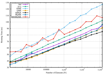
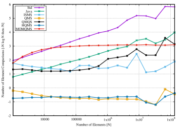
Figure 3. Time (left) and element comparisons (right) for sorting random integer data.

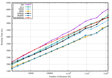
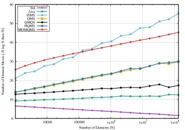
Figure 4. Time for sorting random data with a comparator that applies the logarithm to the integer elements (left), and number of element moves (right).

6. Conclusion

Sorting $n$ elements is one of the most frequently studied subjects in computer science with applications in almost all areas in which efficient programs run.

With variants of QuickMergesort, we contributed sorting algorithms which are able to run faster than Introsort and DualPivotQuicksort even for elementary data. Compared to Introsort, we reduced the leading term $\alpha$ in $\alpha\cdot n\log n+\mathcal{O}(n)$ in the average number of comparisons from $\alpha\approx 1.18$ via $1.09$ to finally reaching 1. The algorithms are simple but effective: a) Median-of-3 pivot selection (as opposed to using a sample of $\sqrt{n}$), b) faster sorting for smaller element sets. Both modifications show empirical impact and are analyzed theoretically to provide upper bounds on the average number of comparisons. We discussed options to warrant a constant-factor optimal worst-case.

In the theoretical part of our work we concentrated on average-case analyses, as we strongly believe that this reflects realistic behavior more closely than worst-case analyses. With very low overhead, QuickMergesort has implemented in a way that it becomes constant-factor optimal in the worst-case, too. We chose efficient deterministic median-of-median strategies that are also of interest for further considerations.

For future research we propose the integration of QuickMergesort with multi-way merging, envisioning to scale the algorithm beyond main memory capacity and effective parallelizations.

References

- [1] Andrei Alexandrescu. Fast deterministic selection. In 16th International Symposium on Experimental Algorithms, SEA 2017, June 21-23, 2017, London, UK, pages 24:1–24:19, 2017.
- [2] Martin Aumüller and Martin Dietzfelbinger. Optimal partitioning for dual pivot quicksort - (extended abstract). In ICALP, pages 33–44, 2013.
- [3] Martin Aumüller, Martin Dietzfelbinger, and Pascal Klaue. How good is multi-pivot quicksort? CoRR, abs/1510.04676, 2015.
- [4] Manuel Blum, Robert W. Floyd, Vaughan R. Pratt, Ronald L. Rivest, and Robert E. Tarjan. Time bounds for selection. Journal of Computer and System Sciences, 7(4):448–461, 1973.
- [5] D. Cantone and G. Cinotti. QuickHeapsort, an efficient mix of classical sorting algorithms. Theoretical Computer Science, 285(1):25–42, 2002.
- [6] Thomas H. Cormen, Charles E. Leiserson, Ronald L. Rivest, and Clifford Stein. Introduction to Algorithms. The MIT Press, 3th edition, 2009.
- [7] Volker Diekert and Armin Weiß. Quickheapsort: Modifications and improved analysis. In CSR, pages 24–35, 2013.
- [8] Ronald D. Dutton. Weak-heap sort. BIT, 33(3):372–381, 1993.
- [9] Stefan Edelkamp and Armin Weiß. QuickXsort: Efficient sorting with n logn - 1.399n + o(n) comparisons on average. In CSR, pages 139–152, 2014.
- [10] Stefan Edelkamp and Armin Weiß. Blockquicksort: Avoiding branch mispredictions in Quicksort. In Piotr Sankowski and Christos D. Zaroliagis, editors, 24th Annual European Symposium on Algorithms, ESA 2016, August 22-24, 2016, Aarhus, Denmark, volume 57 of LIPIcs, pages 38:1–38:16. Schloss Dagstuhl - Leibniz-Zentrum für Informatik, 2016.
- [11] Amr Elmasry, Jyrki Katajainen, and Max Stenmark. Branch mispredictions don’t affect mergesort. In SEA, pages 160–171, 2012.
- [12] Robert W. Floyd. Algorithm 245: Treesort 3. Comm. of the ACM, 7(12):701, 1964.
- [13] Jr. Ford, Lester R. and Selmer M. Johnson. A tournament problem. The American Mathematical Monthly, 66(5):pp. 387–389, 1959.
- [14] C. A. R. Hoare. Algorithm 65: Find. Commun. ACM, 4(7):321–322, July 1961.
- [15] Charles A. R. Hoare. Quicksort. The Computer Journal, 5(1):10–16, 1962.
- [16] Kanela Kaligosi and Peter Sanders. How branch mispredictions affect quicksort. In ESA, pages 780–791, 2006.
- [17] Jyrki Katajainen. The ultimate heapsort. In Computing: The Fourth Australasian Theory Symposium (CATS), pages 87–96, 1998.
- [18] Jyrki Katajainen, Tomi Pasanen, and Jukka Teuhola. Practical in-place mergesort. Nord. J. Comput., 3(1):27–40, 1996.
- [19] Donald E. Knuth. Sorting and Searching, volume 3 of The Art of Computer Programming. Addison Wesley Longman, 2nd edition, 1998.
- [20] Shrinu Kushagra, Alejandro López-Ortiz, Aurick Qiao, and J. Ian Munro. Multi-pivot quicksort: Theory and experiments. In ALENEX, pages 47–60, 2014.
- [21] Conrado Martínez, Daniel Panario, and Alfredo Viola. Adaptive sampling strategies for quickselects. ACM Trans. Algorithms, 6(3):53:1–53:45, 2010.
- [22] Conrado Martínez and Salvador Roura. Optimal Sampling Strategies in Quicksort and Quickselect. SIAM J. Comput., 31(3):683–705, 2001.
- [23] David R. Musser. Introspective sorting and selection algorithms. Software—Practice and Experience, 27(8):983–993, 1997.
- [24] Peter Sanders and Sebastian Winkel. Super scalar sample sort. In ESA, pages 784–796, 2004.
- [25] Ingo Wegener. The worst case complexity of McDiarmid and Reed’s variant of bottom-up-heap sort is less than . In STACS, pages 137–147, 1991.
- [26] Ingo Wegener. Bottom-up-Heapsort, a new variant of Heapsort beating, on an average, Quicksort (if is not very small). Theoretical Computer Science, 118:81–98, 1993.
- [27] Sebastian Wild, Markus E. Nebel, and Ralph Neininger. Average case and distributional analysis of dual-pivot quicksort. ACM Transactions on Algorithms, 11(3):22:1–22:42, 2015.
- [28] J. W. J. Williams. Algorithm 232: Heapsort. Communications of the ACM, 7(6):347–348, 1964.