MPGM: Scalable and Accurate
Multiple Network Alignment

Abstract

Protein-protein interaction (PPI) network alignment is a canonical operation to transfer biological knowledge among species. The alignment of PPI-networks has many applications, such as the prediction of protein function, detection of conserved network motifs, and the reconstruction of species’ phylogenetic relationships. A good multiple-network alignment (MNA), by considering the data related to several species, provides a deep understanding of biological networks and system-level cellular processes. With the massive amounts of available PPI data and the increasing number of known PPI networks, the problem of MNA is gaining more attention in the systems-biology studies.

In this paper, we introduce a new scalable and accurate algorithm, called MPGM, for aligning multiple networks. The MPGM algorithm has two main steps: (i) SeedGeneration and (ii) MultiplePercolation. In the first step, to generate an initial set of seed tuples, the SeedGeneration algorithm uses only protein sequence similarities. In the second step, to align remaining unmatched nodes, the MultiplePercolation algorithm uses network structures and the seed tuples generated from the first step. We show that, with respect to different evaluation criteria, MPGM outperforms the other state-of-the-art algorithms. In addition, we guarantee the performance of MPGM under certain classes of network models. We introduce a sampling-based stochastic model for generating $k$ correlated networks. We prove that for this model if a sufficient number of seed tuples are available, the MultiplePercolation algorithm correctly aligns almost all the nodes. Our theoretical results are supported by experimental evaluations over synthetic networks.

1 Introduction

Protein-protein interaction (PPI) networks are a valuable source of information for understanding the evolution of protein interactions and system-level cellular processes. Discovering and predicting the interaction patterns, which are related to the functioning of cells, is a fundamental goal in studying the topology of PPI networks. A comparative analysis of PPI networks provides us insight into the evolution of species and can help us to transfer biological knowledge across species.

Network alignment is one of the most powerful methods for comparing PPI networks. The main goal of network alignment is to find functionally orthologous proteins and to detect conserved pathways and protein complexes among different species. Local network-alignment and global network-alignment are the two general classes of network-alignment algorithms. The local network-alignment algorithms search for small but highly conserved sub-networks (e.g., homologous regions of biological pathways or protein complexes) among species by comparing PPI networks locally. The global network-alignment algorithms instead, by maximizing the overall similarity of networks, try to align all (or most of) the proteins to find large sub-graphs that are functionally and structurally conserved over all the nodes in the two (or several) networks.

The advance of high-throughput methods for detecting protein interactions has made the PPI networks of many organisms available to researchers. With the huge amounts of biological network data and the increasing number of known PPI networks, the problem of multiple-network alignment (MNA) is gaining more attention in the systems-biology studies. We believe that a good MNA algorithm leads us to a deeper understanding of biological networks (compared to pairwise-network alignment methods) because they capture the knowledge related to several species. Most of the early works on global PPI-network alignment consider matching only two networks Singh et al. (2007); Ahmet Emre Aladag and Cesim Erten (2013); Neyshabur et al. (2013); Hashemifar and Xu (2014); Vijayan et al. (2015); Malod-Dognin and Pržulj (2015); Meng et al. (2016); Kazemi and Grossglauser (2016).

MNA methods produce alignments consisting of aligned tuples with nodes from several networks. MNA algorithms are classified into two categories of one-to-one and many-to-many algorithms. In the first category, each node from a network can be aligned to at most one node from another network. In the many-to-many category, one or several nodes from a network can be aligned with one or several nodes from another network.

Several MNA algorithms were proposed in the past few years: NetworkBlast-M, a many-to-many local MNA algorithm, begins the alignment process with a set of high-scoring sub-networks (as seeds). It then expands them in a greedy fashion Sharan et al. (2005); Kalaev et al. (2008). Graemlin Flannick et al. (2006) is a local MNA algorithm that finds alignments by successively performing alignments between pairs of networks, by using information from their phylogenetic relationship. IsoRankN Liao et al. (2009) is the first global MNA algorithm that uses both pairwise sequence similarities and network topology, to generate many-to-many alignments. SMETANA Sahraeian and Yoon (2013), another many-to-many global MNA algorithm, tries to find aligned node-tuples by using a semi-Markov random-walk model. This random-walk model is used for computing pairwise similarity scores. CSRW Jeong and Yoon (2015), a modified version of SMETANA, uses a context-sensitive random-walk model. NetCoffee Hu et al. (2014) uses a triplet approach, similar to T-Coffee Notredame et al. (2000), to produce a one-to-one global alignment. GEDEVO-M Ibragimov et al. (2014) is a heuristic one-to-one global MNA algorithm that uses only topological information. To generate multiple alignments, GEDEVO-M minimizes a generalized graph edit distance measure. NH Radu and Charleston (2015) is a many-to-many global MNA heuristic algorithm that uses only network structure. Alkan and Erten Alkan and Erten (2014) designed a many-to-many global heuristic method based on a backbone extraction and merge strategy (BEAMS). The BEAMS algorithm, given $k$ networks, constructs a $k$-partite pairwise similarity graph. It then builds an alignment, in a greedy manner, by finding a set of disjoint cliques over the $k$-partite graph. Gligorijević et al. Gligorijević et al. (2015) introduced FUSE, another one-to-one global MNA algorithm. FUSE first applies a non-negative matrix tri-factorization method to compute pairwise scores from protein-sequence similarities and network structure. Then it uses an approximate $k$-partite matching algorithm to produce the final alignment.

In this paper, we introduce a new scalable and accurate one-to-one global multiple-network alignment algorithm called MPGM (Multiple Percolation Graph Matching). The MPGM algorithm has two main steps. In the first step (SeedGeneration, it uses only protein sequence similarities to generate an initial set of seed tuples. In the second step (MultiplePercolation), it uses the structure of networks and the seed tuples generated from the first step to align remaining unmatched nodes. MPGM is a new member of the general class of percolation graph matching (PGM) algorithms Narayanan and Shmatikov (2009); Yartseva and Grossglauser (2013); Korula and Lattanzi (2014); Chiasserini et al. (2015b); Kazemi et al. (2015a).

The PGM algorithms begin with the assumption that there is side information provided in the form of a set of pre-aligned node couples, called seed set. These algorithms assume that a (small) subset of nodes between the two networks are identified and aligned a priori. The alignment is generated through an incremental process, starting from the seed couples and percolating to other unmatched node couples based on some local structural information. More specifically, in every step, the set of aligned nodes are used as evidence to align additional node couples iteratively. The evidence for deciding which couple to align can take different forms, but it is obtained locally within the two networks Yartseva and Grossglauser (2013); Kazemi (2016). The PGM algorithms are truly scalable to graphs with millions of nodes and are robust to large amount of noise Korula and Lattanzi (2014); Kazemi et al. (2015a).

MPGM is the first algorithm from the powerful class of PGM algorithms that aligns more than two networks. Our MNA algorithm is designed based on ideas inspired by PROPER, a global pairwise-network alignment algorithm Kazemi et al. (2016). We compare MPGM with several state-of-the-art algorithms. We show that MPGM outperforms the other algorithms, with respect to different evaluation criteria. Also, we provide experimental evidence for the good performance of the SeedGeneration algorithm. Finally, we study, theoretically and experimentally, the performance of the MultiplePercolation algorithm, by using a stochastic graph-sampling model.

2 Algorithms and Methods

The goal of a one-to-one global MNA algorithm is to find an alignment between proteins from $k$ different species (networks), where a protein from one species can be aligned to at most one unique protein from another species, in such a way that (i) the tuples of aligned proteins have similar biological functions, and (ii) the aligned networks are structurally similar, e.g., they share many conserved interactions among different tuples. To be more precise, a one-to-one global alignment $\pi$ between $k$ networks $G_{i}=(V_{i},E_{i}),1\leq i\leq k$, is the partition of all (or most of) the nodes $V=\cup_{i=i}^{k}V_{i}$ into tuples $\{T_{1},T_{2},\cdots,T_{|\pi|}\}$, where each tuple is of size at least two (i.e., they should have nodes from at least two networks), and where each tuple $T_{i}$ has at most one node from each network. In addition, any two tuples $T_{i}$ and $T_{j}$ are disjoint, i.e., $T_{i}\cap T_{j}=\emptyset$.

In the global MNA problem, to align the proteins from $k>2$ species, PPI-networks and protein sequence similarities are used as inputs. Formally, we are given the PPI networks of $k$ different species: the networks are represented by $G_{1}(V_{1},E_{1}),G_{2}(V_{2},E_{2}),\cdots,G_{k}(V_{k},E_{k})$. Also, the BLAST sequence similarity of the couples of proteins in all the $\binom{k}{2}$ pairs of species is provided as additional side information. The BLAST bits-score similarity for two proteins $u$ and $v$ is represented by $BlastBit(u,v)$. Let $\mathcal{S}_{\geq\ell}$ denote the set of all couples with BLAST bit-score similarity of at least $\ell$, i.e., $\mathcal{S}_{\geq\ell}=\{[u,v]\in\cup_{1\leq i<j\leq k}V_{i}\times V_{j}\ |\ BlastBit(u,v)\geq\ell\}$. Next, we introduce MPGM, our proposed global MNA algorithm.

2.1 The MPGM Algorithm

The MPGM algorithm has two main steps: (i) In the first step, it uses only the sequence similarities to find a set of initial seed-tuples. These seed tuples have nodes from at least two networks. (ii) In the second step, by using the network structure and the seed-tuples (generated from the first step), MPGM, aligns the remaining unmatched nodes with a percolation-based graph-matching algorithm. Specifically, in the second step, MPGM adds new nodes to the initial set of seed-tuples, by using only structural evidence, to generate larger and new tuples.

2.1.1 First Step: SeedGeneration

We now explain how to generate the seed-tuples $\mathcal{A}=\{T_{1},T_{2},\cdots,T_{|\mathcal{A}|}\}$, by using only sequence similarities. We first define an $\ell$-consistent tuple as a natural candidate for seed set. Then, to find these $\ell$-consistent tuples, we introduce a heuristic algorithm, called SeedGeneration.

Definition 1.

A tuple $T$ is $\ell$-consistent, if for every $u\in T$ there is at least one other protein $v\in T$ ($u$ and $v$ are from two different networks), such that $BlastBit(u,v)\geq\ell$.

In Section 5, (i) we argue that it is reasonable to assume that the BLAST bit-score similarities among real proteins are (pseudo) transitive, and (ii) we show that proteins with high sequence-similarities, often share many experimentally verified GO terms. The pseudo-transitivity property of the BLAST bit-scores guarantees that, in an $\ell$-consistent tuple $T$, almost all the $\binom{|T|}{2}$ pairwise couples have high sequence-similarities; and we know proteins with high sequence-similarities, often have similar biological functions. Therefore, it is likely that all the proteins in an $\ell$-consistent tuple share many biological functions.

In SeedGeneration, we consider only those couples with BLAST bit-score similarity of at least $\ell$, i.e., set $\mathcal{S}_{\geq\ell}$. Note that the parameter $\ell$ is in input to the algorithm. The SeedGeneration algorithm, by processing the protein couples from the highest BLAST bit-score similarity to the lowest, fills in the seed-tuples with proteins from several species in a sequential and iterative procedure. At a given step of SeedGeneration, assume $[u,v]$ is the next couple that we are going to process, where $u$ and $v$ are from the $i$th and $j$th networks, respectively. To add this couple to the seed-tuples $\mathcal{A}$, we consider the following cases: (i) Both $u$ and $v$ do not belong to a tuple in $\mathcal{A}$: we add both nodes to a new tuple, i.e., add $T=[u,v]$ to $\mathcal{A}$. (ii) Only one of $u$ or $v$ belongs to a tuple in $\mathcal{A}$: assume, without loss of generality, $u$ belongs to a tuple $T_{u}$. If the tuple $T_{u}$ does not already have a protein from the network of node $v$ (i.e., $V_{j}$), then $v$ is added to $T_{u}$. This step adds one protein to one existing tuple. (iii) Both $u$ and $v$, respectively, belong to tuples $T_{u}$ and $T_{v}$ in $\mathcal{A}$: If $T_{u}$ and $T_{v}$ do not yet have a node from the $j$th and $i$th networks, respectively, then we merge $T_{u}$ and $T_{v}$ by the MergeTuples algorithm.

The goal of MergeTuples is to combine the two tuples in order to generate a larger tuple that has nodes from more networks. In this merging algorithm, it is possible to have another (small) tuple as a leftover. In words, MergeTuples picks the tuple that contains the couple with the highest sequence similarity (refer to it as $T_{1}$). If the other tuple (denote by $T_{2}$) has nodes from networks that $T_{1}$ did not have a node form them, MergeTuples adds those nodes to $T_{1}$. In this way, we can generate a tuple with nodes from more networks. At the end of this process if $T_{2}$ has less than two nodes we will delete it. Algorithm 1 describes SeedGeneration. Also, MergeTuples is described in Algorithm 2. For the notations used in the paper refer to Table 5 in Appendix A.

1:$\mathcal{S}_{\geq\ell}$ (the set of all couples with BLAST bit-score similarity at least $\ell$)

2:The seed set $\mathcal{A}$ of tuples

3:for all pairs $[u,v]$ in $\mathcal{S}_{\geq\ell}$ from the most similar to the lowest  $\triangleright$ If there are several pairs with the same BLAST bit-score we randomly pick one of them randomly. do

4:     Assume $u\in V_{i}$ and $v\in V_{j}$

5:     if $\mathcal{A}(u)=\emptyset$ and $\mathcal{A}(v)=\emptyset$ then

6:         Add tuple $T=[u,v]$ to $\mathcal{A}$

7:     else if $\mathcal{A}(u)\neq\emptyset$ and $\mathcal{A}(v)=\emptyset$ then

8:         if $V_{j}\cap\mathcal{A}(u)=\emptyset$ then

9:              add $v$ to the tuple $\mathcal{A}(u)$

10:         end if

11:     else if $\mathcal{A}(u)=\emptyset$ and $\mathcal{A}(v)\neq\emptyset$ then

12:         if $V_{i}\cap\mathcal{A}(v)=\emptyset$ then

13:              add $u$ to the tuple $\mathcal{A}(v)$

14:         end if

15:     else

16:         if $V_{j}\cap\mathcal{A}(u)=\emptyset$ and $V_{i}\cap\mathcal{A}(v)=\emptyset$ then

17:              MergeTuples $(\mathcal{A}(u),\mathcal{A}(v))$

18:         end if

19:     end if

20:end for

21:return $\mathcal{A}$ 

Algorithm 1 The SeedGeneration algorithm

1:Two tuples $T_{1}$ and $T_{2}$

2:The modified tuples $T_{1}$ and $T_{2}$

3:Without loss of generality assume $T_{1}$ is the tuple that contains the couple with the highest sequence similarity

4:for i = 1 to k do

5:     if $V_{i}\cap T_{1}=\emptyset$ and $V_{i}\cap T_{2}\neq\emptyset$ then

6:         Move node $V_{i}\cap T_{2}$ from tuple $T_{2}$ to tuple $T_{1}$

7:     end if

8:end for

9:if $|T_{2}|\leq 1$ then

10:     Delete the tuple $T_{2}$

11:end if

Algorithm 2 The MergeTuples algorithm

Example 2.

Table 1 shows a sample execution of the SeedGeneration algorithm. This algorithm uses the set of pairwise sequence similarities; this set is sorted from the highest BLAST bit-score to $\ell$.

Table 1: An example of the SeedGeneration algorithm. Inputs to this algorithm are the set of pairwise sequence-similarities (i.e, $BlastBit(\cdot,\cdot)$) and a fixed threshold $\ell$. The sequence similarities are sorted from the highest BLAST bit-score to $\ell$. The seed-tuples $\mathcal{A}$ are generated from the pairwise similarities. In this example, the couple [hs1, mm8] (i.e., the couple of proteins with the highest sequence similarity) generates the first tuple in the seed set. At the third step, one of the nodes from the third couple, i.e., hs1, is already in the tuple $T_{1}=$[hs1, mm8]. Because $T_{1}$ does not have any node from the network of ce, the node ce4 is added to $T_{1}$. Also at the eight step, as the two nodes from [ce6, hs9] belong to two different tuples, their corresponding tuples are merged.

$\#$	Couples	BLAST	Seed-tuples $\mathcal{A}$
1	[hs1, mm8]	1308	[hs1, mm8]
2	[ce6, sc9]	909	[hs1, mm8] and [ce6,  sc9]
3	[ce4, hs1]	813	[ce4, hs1, mm8] and [ce6, sc9]
4	[dm15, mm8]	797	[ce4, dm15, hs1, mm8] and [ce6, sc9]
5	[ce654, mm8]	603	[ce4, dm15, hs1, mm8] and [ce6, sc9]
6	[dm15, sc12]	414	[ce4, dm15, hs1, mm8, sc12] and [ce6, sc9]
7	[dm7, hs9]	334	[ce4, dm15, hs1, mm8, sc12], [ce6, sc9] and [dm7, hs9]
8	[ce6, hs9]	282	[ce4, dm15, hs1, mm8, sc12] and [ce6, dm7, hs9, sc9]
9	[dm7, sc63]	101	[ce4, dm15, hs1, mm8, sc12] and [ce6, dm7, hs9, sc9]

2.1.2 Second Step: MultiplePercolation

In the second step of MPGM, a new PGM algorithm, called MultiplePercolation, uses the network structures and the generated seed-tuples from the first step, to align the remaining unmatched nodes. This PGM algorithm uses the structural similarities of couples as the only evidence for matching new nodes. The MultiplePercolation algorithm adds new tuples in a greedy way, in order to maximize the number of conserved interactions among networks. In MultiplePercolation, network structure provides evidence for similarities of unmatched node-couples, and a couple with enough structural similarity is matched. New node-tuples are generated by merging matched couples. Also, if there is enough structural similarity between two nodes from different tuples, the two tuples are merged. In the MultiplePercolation algorithm, we look for tuples that contain nodes from more networks, i.e., a tuple that has nodes from more networks is more valuable. Next, we explain the MultiplePercolation algorithm in detail.

Assume $\pi$ is the set of aligned tuples at a given time step of the MultiplePercolation algorithm. Note that we have initially $\pi=\mathcal{A}$, where $\mathcal{A}$ is the output of SeedGeneration. Let $\pi_{i,j}$ denotes the set of pairwise alignments between nodes from the $i$th and $j$th networks: A couple $[u,v]$, where $u\in V_{i}$ and $v\in V_{j}$, belongs to the set $\pi_{i,j}$, if and only if there is a tuple $T\in\pi$ such that both $u$ and $v$ are in that tuple. The set $\pi_{i,j}$ is defined as

$$\pi_{i,j}=\{[u,v]| u\in V_{i}\ \text{ and}\ v\in V_{j}\$$

$$\text{such that there exists}\ T\in\pi\ \text{where}\ u,v\in T\}.$$

The score of a couple of nodes is the number of their common neighbors in the set of previously aligned tuples. Formally, we define the score of a couple $[u,v],u\in V_{i}\ \text{and}\ v\in V_{j}$ as

$$score([u,v])= |\{[u^{\prime},v^{\prime}]\in\pi_{i,j}$$

$$\text{such that}\ (u,u^{\prime})\in E_{i}\ \text{and}\ (v,v^{\prime})\in E_{j}\}|.$$

In other words, the score of a couple is equal to the number of interactions that remain conserved if this couple is added as a new tuple to the set of currently aligned tuples. Assigning the score to a couple is a way to quantify the structural similarity between two nodes of that couple. Alternatively, it is possible to interpret the score of a couple as follows: All the couples $[u,v]\in\pi_{i,j}$ provide marks for their neighboring couples, i.e., the couples in $N_{i}(u)\times N_{j}(v)$ receive one mark from $[u,v]$, where $N_{i}(u)$ denotes the set of neighbors of node $u$ in $G_{i}$. The score of a couple is the number of marks it has received from the previously aligned couples (note that aligned couples are subsets of the aligned tuples). In the MultiplePercolation algorithm, the initial seed-tuples provide structural evidence for the other unmatched couples. Indeed, for a tuple $T$, all the $\binom{|T|}{2}$ possible couples $[u,v]$, which are subsets of $T$, spread marks to their neighboring couples in the networks $V(u)$ and $V(v)$, where $V(u)$ denotes the network $V$ such that $u\in V$.

After the initial mark spreading step, the couple $[u,v]$ with the highest number of marks (but at least $r$) is the next candidate to get matched. The alignment process is as follows: (i) If $\pi(u)=\emptyset$ and $\pi(v)=\emptyset$, then we add a new tuple $T=[u,v]$ to the set of previously aligned tuples $\pi$. (ii) If exactly one of the two nodes $u$ or $v$ belongs to a tuple $T\in\pi$, by adding the other node to $T$ (if it is possible), we generate a tuple with nodes from one more network. (iii) If both $u$ and $v$ belong to different tuples of $\pi$, by merging these two tuples (again, if possible), we make a larger tuple.

After the alignment process, $[u,v]$ spreads out marks to the other couples, because it is a newly matched couple. Then, recursively new couples are matched and added to the set of aligned tuples. The alignment process continues to the point that there is no couple with a score of at least $r$. Algorithm 3 describes MultiplePercolation. For the notations refer to Table 5 in Appendix A.

1:$G_{1}(V_{1},E_{1}),G_{2}(V_{2},E_{2}),\cdots,G_{k}(V_{k},E_{k})$ seed tuples $\mathcal{A}$ and the threshold $r$

2:The set of aligned tuples $\pi$

3:$\pi\leftarrow\mathcal{A}$

4:The tuples in set $\mathcal{A}$ spread out marks to their neighboring couples

5:while there exists a couple with score at least $r$ do  $\triangleright$ While a new tuple is generated or a new node is added to a tuple the marks from those newly aligned couples are spread over their neighboring couples.

6:     $[u,v]\leftarrow$ the couple with the highest score, where $u\in V_{i}$ and $v\in V_{j}$

7:     if $\pi(u)=\emptyset$ and $\pi(v)=\emptyset$ then

8:         Add tuple $T=[u,v]$ to $\pi$

9:     else if $\pi(u)\neq\emptyset$ and $\pi(v)=\emptyset$ then

10:         if $V_{j}\cap\pi(u)=\emptyset$ then

11:              Add $v$ to tuple $\pi(u)$

12:         end if

13:     else if $\pi(u)=\emptyset$ and $\pi(v)\neq\emptyset$ then

14:         if $V_{i}\cap\pi(v)=\emptyset$ then

15:              Add $u$ to tuple $\pi(v)$

16:         end if

17:     else

18:         if  for all $V_{\ell,1\leq\ell\leq k}$ we have $V_{\ell}\cap\pi(u)={}\emptyset$ or $V_{\ell}\cap\pi(v)={}\emptyset$  then

19:              Merge the two tuples $\pi(u)$ and $\pi(v)$

20:         end if

21:     end if

22:end while

23:return $\pi$ 

Algorithm 3 MultiplePercolation

Example 3.

Figure 1 provides an example of the MultiplePercolation algorithm over graphs $G_{1,2,3}$. Dark-green nodes are the initial seed-tuples. The tuple $[x_{1},x_{2},x_{3}]$ is an example of a seed tuple that contains nodes from all the three networks. $[y_{1},y_{2}]$ is a seed couple between networks $G_{1}$ and $G_{2}$. All the pairwise couples, which are subsets of the initial seed-tuples, provide structural evidence for the other nodes. In this example, after that initial seed-tuples spread out marks to other couples, the couples $[w_{1},w_{2}]$ and $[u_{2},u_{3}]$ have the highest score (their score is three). Hence we align them first. Among the couples with score two, $[w_{1},u_{3}]$ is not a valid alignment; because the nodes $w_{1}$ and $u_{3}$ are matched to different nodes in $G_{2}$ (also, this true for $w_{2}$ and $u_{2}$). The set of aligned tuples is $\{[u_{1},u_{2},u_{3}],[v_{1},v_{2},v_{3}],[w_{1},w_{2}],[z_{2},z_{3}]\}$. Here, there is not enough information to match $v_{1}$ and $v_{3}$ directly, but as they both are matched to $v_{2}$, we can align them through transitivity of the alignments. Furthermore, if we continue the percolation process, it is possible to match the couples $[i_{1},i_{2}]$ and $[i_{1},i_{3}]$; it results in the tuple $[i_{1},i_{2},i_{3}]$. Note that, by aligning all the networks at the same time, we have access to more structural information. For example, although the pairwise alignment of $G_{1}$ and $G_{3}$ does not provide enough evidence to align $[v_{1},v_{3}]$, it is possible to align this couple by using the side information we can get through $G_{2}$.

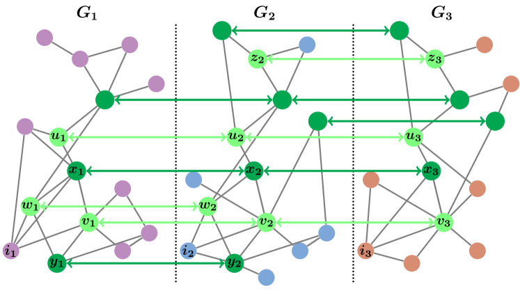
Figure 1: The alignment is performed over graphs $G_{1}$, $G_{2}$ and $G_{3}$. Dark-green nodes are the initial seed-tuples. Light-green nodes are tuples that are matched in the PGM process.

3 Performance Measures

Comparing global MNA algorithms is a challenging task for several reasons. Firstly, it is not possible to directly evaluate the performance of algorithms, because the true node mappings for real biological networks is not known. Secondly, algorithms can return tuples of different sizes. Although the fundamental goal of a global MNA algorithm is to find tuples with nodes from many different networks, some algorithms tend to return tuples of smaller sizes. Therefore, tuples of different sizes make the comparison more difficult. For these reasons, we use several measures in the literature. In addition, we introduce a new measure, using the information content of aligned tuples.

We first compare global MNA algorithms based on their performance in generating large tuples. The best tuples are those that contain nodes from all $k$ networks, whereas tuples with nodes from only two networks are worst Gligorijević et al. (2015). The $d$-coverage of tuples denotes the number of tuples with nodes from exactly $d$ networks Gligorijević et al. (2015). Note that for many-to-many alignment algorithms, it is possible to have more than $d$ nodes in a tuple with nodes from $d$ networks. Therefore, for the number of proteins in tuples with different $d$-coverages, we also consider the total number of nodes in those tuples Gligorijević et al. (2015).

The first group of measures evaluates the performance of algorithms using the functional similarity of aligned proteins. A tuple is annotated if it has at least two proteins annotated with at least one GO term Gligorijević et al. (2015). An annotated tuple is consistent if all of the annotated proteins in that tuple share at least one GO term. We define $\#AC$ as the total number of annotated tuples. Furthermore, $\#AC_{d}$ represents the number of annotated tuples with a coverage $d$. For the number of consistent tuples, we define $\#CC$ and $\#CC_{d}$ similarly. Also, the number of proteins in a consistent tuple with coverage $d$ is denoted by $\#CP_{d}$. The specificity of an alignment is defined as the ratio of the number of consistent tuples to the number of annotated tuples: $Spec=\tfrac{\#CC}{\#AC}$ and $Spec_{d}=\tfrac{\#CC_{d}}{\#AC_{d}}$ Gligorijević et al. (2015).

Mean entropy (ME) and mean normalized entropy (MNE) are two other measures that calculate the consistency of aligned proteins by using GO terms Liao et al. (2009); Sahraeian and Yoon (2013); Alkan and Erten (2014). The entropy (E) of a tuple $T=[p_{1},p_{2},\cdots,p_{d}]$, with the set of GO terms $GO(T)=\{GO_{1},GO_{2},\cdots,GO_{m}\}$, is defined as $E(T)=-\sum_{i=1}^{m}g_{i}\log{g_{i}},$ where $g_{i}$ is the fraction of proteins in $T$ that are annotated with the GO term $GO_{i}$. ME is defined as the average of $E(T)$ over all the annotated tuples. Normalized entropy (NE) is defined as $NE(T)=\frac{1}{\log m}E(T),$ where $m$ is the number of different GO terms in tuple $T$. Similarly, MNE is defined as the average of $NE(T)$ over all the annotated tuples.

To avoid the shallow annotation problem, Alkan and Erten (2014) and Gligorijević et al. (2015) suggest to restrict the protein annotations to the fifth level of the GO directed acyclic graph (DAG): (i) by ignoring the higher level GO annotations, and (ii) by replacing the deeper-level GO annotations with their ancestors at the fifth level. For the specificity ($Spec$ and $Spec_{d}$) and entropy (ME and MNE) evaluations, we use the same restriction method.

The way we deal with the GO terms can greatly affect the comparison results. Indeed, there are several drawbacks with the restriction of the GO annotations to a specific level. Firstly, although depth is one of the indicators of specificity, the GO terms that are at the same level do not always have same semantic precision, and a GO term at a higher level might be more specific than a term at a lower level Resnik (1999). Also, it is known that the depth of a GO term reflects mostly the vagaries of biological knowledge, rather than anything intrinsic about the terms Lord et al. (2003). Secondly, there is no explanation (e.g., in Alkan and Erten (2014); Gligorijević et al. (2015)) about why we should restrict the GO terms to the fifth level. Also, the notion of consistency for a tuple (i.e., sharing at least one GO term) is very general and does not say anything about how specific the shared GO terms are. Furthermore, from our experimental studies, we observe that two random proteins share at least one experimentally verified GO term with probability $0.21$, whereas five proteins share at least one GO term with a very low probability of $0.002$.

To overcome these limitations, we define the semantic similarity ($SS_{p}$) measure for a tuple of proteins. This is the generalization of a measure that is used for the semantic similarity of two proteins Resnik (1999); Schlicker and Albrecht (2008). Assume $|annot(t_{i})|$ is the number of proteins that are annotated with the GO term $t_{i}$. The frequency of $t_{i}$ is defined as $freq(t_{i})=|annot(t_{i})|+\sum_{s\in successors(t_{i})}|annot(s)|,$ where $successors(t_{i})$ is the successors of the term $t_{i}$ in its corresponding gene-annotation DAG. The relative frequency $p(t_{i})$ for a GO term $t_{i}$ is defined as $p(t_{i})=\tfrac{freq(t_{i})}{freq(root)}$. The information content (IC) Resnik (1999) for a term $t_{i}$ is defined as $IC(t_{i})=-\log(p(t_{i}))$. The semantic similarity between the $d$ terms $\{t_{1},t_{2},\cdots,t_{d}\}$ is defined as $SS(t_{1},t_{2},\cdots,t_{d})=IC(LCA(t_{1},t_{2},\cdots,t_{d})),$ where $LCA(t_{1},t_{2},\cdots,t_{d})$ is the lowest common ancestor of terms $t_{i}$ in DAG. For proteins ${p_{1},p_{2},\cdots,p_{d}}$, we define semantic similarity as

$$SS_{p}(p_{1},p_{2},\cdots,p_{d})=$$

$$\max_{t_{1}\in GO(p_{1}),t_{2}\in GO(p_{2}),\cdots,t_{d}\in GO(p_{d})}IC(LCA(t_{1},t_{2},\cdots,t_{d})),$$ (1)

where $GO(p_{i})$ are the GO annotations of $p_{i}$. The sum of $SS_{p}$ values for all tuples in an alignment $\pi$ is shown by $SS_{p}(\pi)$. Let $\overline{SS_{p}}(\pi)$ denote the average of $SS_{p}$ values, i.e., $\overline{SS_{p}}(\pi)=\frac{SS_{p}(\pi)}{|\pi|}$. Note that, algorithms with higher values of $SS_{p}(\pi)$ and $\overline{SS_{p}}(\pi)$, result in alignments with higher qualities, because these alignments contain tuples with more specific functional similarity among their proteins.

The second group of measures evaluates the performance of global MNA algorithms based on the structural similarity of aligned networks. We define edge correctness (EC) as a generalization of the measures introduced in Kuchaiev et al. (2010); Patro and Kingsford (2012). EC is a measure of edge conservation between aligned tuples under a multiple alignment $\pi$. For two tuples $T_{i}$ and $T_{j}$, let $E_{T_{i},T_{j}}$ denote the set of all the interactions between nodes from these two tuples, i.e., $E_{T_{i},T_{j}}=\{e=(u,v)|u\in T_{i},v\in T_{j}\}$. The set of networks that have an edge in $E_{T_{i},T_{j}}$ is defined as $V(E_{T_{i},T_{j}})$. Theoretically, we can have a conserved interaction between two tuples $T_{i}$ and $T_{j}$, if they have nodes from at least two similar networks, i.e., $|V(T_{i})\cap V(T_{j})|\geq 2$. The interaction between two tuples $T_{i}$ and $T_{j}$ is conserved if there are at least two edges from two different networks between these tuples, i.e., $|V(E_{T_{i},T_{j}})|\geq 2$. The EC measure is defined as $EC(\pi)=\tfrac{\Delta(\pi)}{E(\pi)},$ where $E(\pi)$ is the total number edges between all the tuples $T_{i}$ and $T_{j}$, such that $|V(T_{i})\cap V(T_{j})|\geq 2$. Also, $\Delta(\pi)$ is the total number of edges between those tuples with $|V(E_{T_{i},T_{j}})|\geq 2$. In order to provide further analysis, in two of our experiments we restrict EC to only consistent tuples. Although EC based on consistent tuples is neither topological nor biological, it captures both type of measures in just one.

Cluster interaction quality (CIQ) measures the structural similarity as a function of the conserved interactions between different tuples Alkan and Erten (2014). The conservation score $cs(T_{i},T_{j})$ is defined as

$$cs(T_{i},T_{j})=\begin{cases}0&\text{if}\ |V(T_{i})\cap V(T_{j})|=0\ \text{or}\\ &\qquad\quad\qquad|V(E_{T_{i},T_{j}})|=1\\ \frac{|V(E_{T_{i},T_{j}})|}{|V(T_{i})\cap V(T_{j})|}&\text{otherwise},\end{cases}$$

where $|V(T_{i})\cap V(T_{j})|$ and $|V(E_{T_{i},T_{j}})|$ are the number of distinct networks with nodes in both $T_{i,j}$ and with edges in $E_{T_{i},T_{j}}$, respectively. $CIQ(\pi)$ is defined as:

$$CIQ(\pi)=\frac{\sum_{\forall T_{i},T_{j}\in\pi}|E_{T_{i},T_{j}}|\times cs(T_{i},T_{j})}{\sum_{\forall T_{i},T_{j}\in\pi}|E_{T_{i},T_{j}}|}.$$

We can interpret CIQ as a generalization of $S^{3}$ Saraph and Milenković (2014), a measure for evaluating the structural similarity of two networks.

4 EXPERIMENTS AND EVALUATIONS

We compare MPGM with several state-of-the-art global MNA algorithms: FUSE (F) (Gligorijević et al., 2015), BEAMS (B) (Alkan and Erten, 2014), SMETANA (S) (Sahraeian and Yoon, 2013), CSRW (C) (Jeong and Yoon, 2015), GEDEVO-M (G) Ibragimov et al. (2014) and multiMAGNA++ (M) Vijayan and Milenkovic (2018). Also, we compare our algorithm with IsoRankN (I) (Liao et al., 2009), which is one of the very first global MNA algorithms for PPI networks. For all these algorithms, we used their default settings. Note that IsoRankN, SMETANA, CSRW and BEAMS are many‐to‐many global and, GEDEVO-M, multiMAGNA++ and FUSE are one-to-one algorithms.

Table 2 provides a brief description of the PPI networks for five major eukaryotic species that are extracted from the IntAct database (Hermjakob et al., 2004). The amino-acid sequences of proteins are extracted in the FASTA format from UniProt database (Apweiler et al., 2004). The BLAST bit-score similarities (Altschul et al., 1990) are calculated using these amino-acid sequences. We consider only experimentally verified GO terms, in order to avoid biases induced by annotations from computational methods (mainly from sequence similarities). More precisely, we consider the GO terms with codes EXP, IDA, IMP, IGI and IEP, and we exclude the annotations derived from computational methods and protein-protein interaction experiments. We also consider GO terms from biological process (BP), molecular function (MF) and cellular component (CC) annotations all together.

Table 2: PPI networks of eukaryotic species from IntAct molecular interaction database (Hermjakob et al., 2004).

Species	Abbrev.	$\#$nodes	$\#$edges	Avg. deg.
C. elegans	ce	4950	11550	4.67
D. melanogaster	dm	8532	26289	6.16
H. sapiens	hs	19141	83312	8.71
M. musculus	mm	10765	22345	4.15
S. cerevisiae	sc	6283	76497	24.35

4.1 Comparisons

We first investigate the optimality of SeedGeneration in generating seed-tuples from sequence similarities. To have an upper-bound on the number of proteins in the set of seed-tuples $\mathcal{A}$, we look at the maximum bipartite graph matching between all pairwise species, i.e., all the proteins in all the possible $\binom{k}{2}$ matchings. The total number of nodes that are matched in at least one of these bipartite matchings, provide an upper-bound for the number of matchable nodes. Figure 2 compares SeedGeneration, the proposed upper-bound and MPGM for different values of $\ell$, and the other algorithms based on the total number of aligned proteins. In Figure 3, we compare algorithms based on different $d$-coverages. We observe that MPGM finds the most number of tuples with $5$-coverage among all the algorithms. Furthermore, we observe that MPGM has the best overall coverage (for tuples of size five to two). For example, we also observe that, for $\ell=40$, the SeedGeneration algorithm aligns 28608 proteins (compared to 30820 proteins that we found as an upper-bound) in 1366, 1933, 2342 and 3510 tuples of size 5, 4, 3 and 2, respectively. The second step of MPGM (i.e., MultiplePercolation) extends the initial seed tuples to 40566 proteins aligned in 3076, 2719, 2502 and 3402 tuples of size 5, 4, 3 and 2, respectively. Figures 3 and 4 show, respectively, the number of tuples and proteins in all alignments with different $d$-coverages.

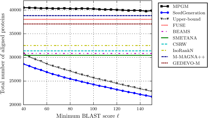
Figure 2: Total number of aligned proteins. For MPGM, we set $r=1$. We observe that MPGM aligns the most number of proteins.

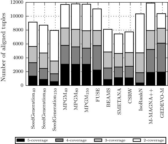
Figure 3: The coverage of alignments.

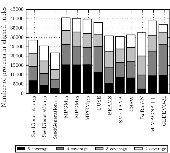
Figure 4: Number of proteins in tuples with different $d$-coverages. The results are for tuples with nodes from five, four, three and two networks. For MPGM, we set $r=1$ and $\ell\in\{40,80,150\}$.

An algorithm with a good $d$-coverage does not necessarily generate high-quality tuples (in terms of functional similarity of proteins). For this reason, we look at the number of consistent tuples. For example, although IsoRankN generates the maximum number of tuples with proteins from two species (see Figure 3), only a small fraction of these tuples are consistent (see Figure 5). Also, in Figure 5, we observe that MPGM returns the largest number of consistent tuples with proteins from five different species. In addition, Figure 6 shows the number of proteins from consistent tuples with different $d$-coverages. In order to further evaluate the functional similarities of aligned proteins, we also used a stronger notion for a consistent tuple: an annotated tuple is strongly consistent if all of the annotated proteins in that tuple share at least two GO terms. In Figure 7 we compare algorithms based on the number of strongly consistent tuples. We observe that SeedGeneration returns the most number of strongly consistent tuples. Also, MPGM performs better than all the other state-of-the-art algorithms.

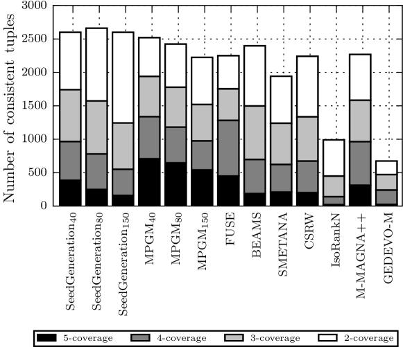
Figure 5: Number of consistent tuples.

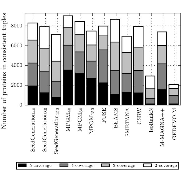
Figure 6: Number of proteins in consistent tuples with different $d$-coverages. The results are for tuples with nodes from five, four, three and two networks. For MPGM, we set $r=1$ and $\ell\in\{40,80,150\}$. We observe that MPGM finds the most number of proteins in consistent tuples and consistent tuple with nodes from all the five networks.

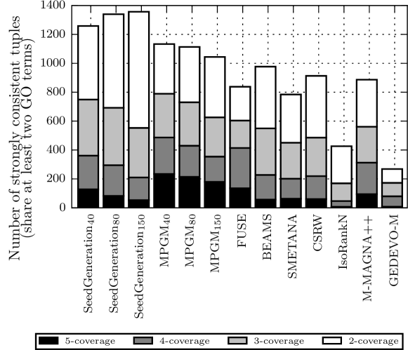
Figure 7: Number of strongly consistent tuples.

In table 3, we compare specificity of algorithms. Note that (i) chance of having better specificity for tuples of smaller sizes is higher, and (ii) different algorithms tend to output alignments with varying distribution of tuple sizes. For this reason, we report specificities of tuples of size $5,4,3$ and $2$ separately. We observe that SeedGeneration provides the alignments with the best specificity. The main reason for this good performance is that it only used the sequence similarity information. Also, the performance of MPGM (in comparison to the other algorithms) is better for larger tuples.

Table 3: Comparison results for specificity of tuples of different sizes. For MPGM we set $r=1$.

	SeedGeneration ($\ell$)			MPGM ($\ell$)			F	B	S	C	I	M	G
	40	80	150	40	80	150
$Spec_{5}$	0.291	0.286	0.284	0.244	0.222	0.184	0.21	0.22	0.187	0.185	0.063	0.194	0.013
$Spec_{4}$	0.339	0.366	0.369	0.277	0.256	0.224	0.299	0.329	0.291	0.306	0.092	0.297	0.075
$Spec_{3}$	0.462	0.486	0.500	0.384	0.382	0.349	0.35	0.437	0.417	0.436	0.153	0.397	0.134
$Spec_{2}$	0.611	0.619	0.646	0.527	0.519	0.529	0.462	0.557	0.558	0.618	0.231	0.495	0.229

Tables 6, 7, 8 and 9 (See Appendix B) provide detailed comparisons for tuples with different coverages. More precisely, Table 6 (Appendix B) compares algorithms over tuples with nodes from five networks. The second step of MPGM (i.e., MultiplePercolation) uses PPI networks to generate 3076 tuples out of initial seed-tuples. We observe that MPGM (for $\ell=40$) finds an alignment with the maximum $d$-coverage, $\#CC_{5}$, $\#CP_{5}$ and $SS_{p}(\pi)$. In addition, the first step of MPGM (i.e., SeedGeneration) has the best performance on $Spec_{5}$, $\overline{SS_{p}}(\pi)$ and MNE. This was expected, because MultiplePercolation uses only network structure, a less reliable source of information for functional similarity in comparison to sequence similarities, to align new nodes. From this table, it is clear that MPGM outperforms the other algorithms with respect to all the measures.

Figure 8 compares algorithms based on the EC measure. We observe that MPGM (for values of $\ell$ larger than 150) finds alignments with the highest EC score. In Figure 9, to calculate EC, we consider only the edges between consistent tuples. We observe that MPGM has the best performance among all the algorithms. This shows that MPGM finds alignments where (i) many of the aligned tuples are consistent and (ii) there are many conserved interactions among these consistent tuples. CIQ is another measure, based on the structural similarity of aligned networks, for further evaluating the performance of algorithms. In Figure 10, we observe that MPGM and SMETANA find alignments with the best CIQ score.

To sum-up, we observe that MPGM generally provides a nice trade-off between functional and structural similarity measures which is the Pareto frontier. That is, one cannot choose an algorithm that does better on both measures. Finally, our recommend setting for MPGM is $r=1$ and $\ell=80$.

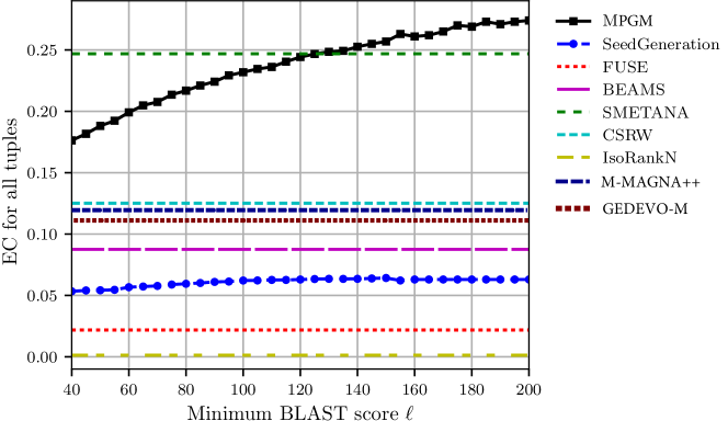
Figure 8: Comparison based on EC for all tuples. The results for MPGM are presented for $r=1$ and different values of $\ell$.

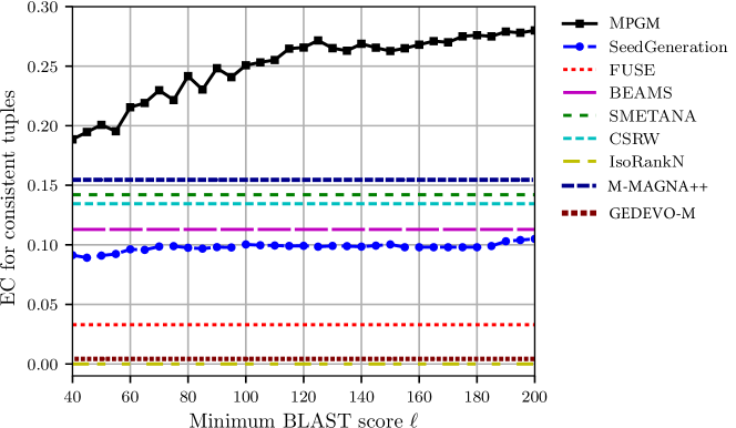
Figure 9: Comparison based on the EC measure for consistent tuples. The results for MPGM are presented for $r=1$ and different values of $\ell$. We observe that MPGM has the best performance among all the algorithms.

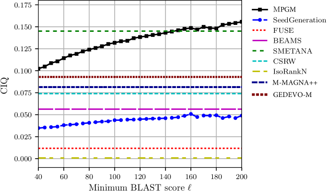
Figure 10: Comparison based on the CIQ measure. The results for MPGM are presented for $r=1$ and different values of $\ell$. We observe that MPGM and SMETANA find alignments with the highest CIQ score.

4.2 Computational Complexity

The computational complexity of the SeedGeneration algorithm is $O\left(|\mathcal{S}_{\geq\ell}|\log{|\mathcal{S}_{\geq\ell}|}\right)$; it includes (i) sorting all the sequence similarities from the highest to the lowest, and (ii) processing them. The computational complexity of the MultiplePercolation algorithm is $O\left(k^{2}\left(|E_{1}|+|E_{2}|\right)\min\left(D_{1},D_{2}\right)\right)$, where $D_{1,2}$ are the maximum degrees in the two networks.

One of the key features of our algorithm is its computational simplicity. MultiplePercolation is easily parallelizable in a distributed manner. To have a scalable algorithm, for very large networks (graphs with millions of nodes), we use a MapReduce Dean and Ghemawat (2008) implementation of MultiplePercolation. The MapReduce programming model consists of two important steps Dean and Ghemawat (2008): First, the Map step processes a subset of data (based on the task) and returns another set of data. Second, the Reduce step, from the result of the Map step, returns a smaller set of data. More specifically, for MultiplePercolation, in the Map step, we spread out marks from the aligned proteins. In the Reduce step, we add all the couples with at least $r$ marks to the set of already aligned proteins $\pi$. The MultiplePercolation algorithm by iteratively performing these two steps aligns the proteins from all the $k$ networks.

In table 4, we compare the time complexity of different algorithms in order to align all the five species form table 2. We observe that MPGM and SMETANA are the fastest algorithms. Also, while FUSE shows the closest performance to MPGM in terms of biological and topological measures, it is much slower. We also evaluated the performance of our MapReduce implementation in scenarios where the original implementation cannot perform the alignment process. For example, by using a Hadoop cluster of 25 nodes, it takes almost 27 minutes to align 5 synthetic networks with 5 million nodes.

Table 4: The time complexity (in seconds) of algorithms for aligning the five species from table 2.

Algorithm	Time (s)
MPGM	131
FUSE	5911
BEAMS	364
SMETANA	146
CSRW	626
IsoRankN	9094
multiMAGNA++	423
GEDEVO-M	4746

5 Interpretation and Discussion

One simple solution to the global MNA problem is to first compute individual alignments between all pairs of networks and then derive the final multiple alignment by merging all these pairwise alignments. The main drawback of this approach is that the collection of these pairwise alignments might be inconsistent. For example, for nodes $u_{1,2,3}\in V_{1,2,3}$, if $u_{1}$ is matched to $u_{2}$ and $u_{2}$ to $u_{3}$, but $u_{1}$ is matched to another node from $G_{3}$, then it is not possible to generate a consistent one-to-one global MNA from these pairwise alignments. In contrast to the idea of merging different pairwise alignments, our approach has three main advantages: (i) It aligns all the $k$ networks at the same time. Therefore, it will always end up with a consistent one-to-one global MNA. (ii) It uses structural information from all networks simultaneously. (iii) The SeedGeneration algorithm gives more weight to the pairs of species that are evolutionarily closer to each other. For example, as H. sapiens and M. musculus are very close, (a) many couples from these two species are matched first, and (b) there are more couples of proteins with high sequence similarities from these two species. Hence there are more tuples that contain proteins from both H. sapiens and M. musculus. In the rest of this section, we provide experimental evidence and theoretical results that explain the good performance of the MPGM algorithm.

5.1 Why Does SeedGeneration Work?

The first step of MPGM (SeedGeneration) is a heuristic algorithm that generates seed-tuples. The SeedGeneration algorithm is designed based on the following observations. First, it is well known that proteins with high BLAST bit-score similarities share GO terms with a high probability. Second, we look at the transitivity of BLAST bit-score similarities for real proteins. Note that the BLAST similarity, in general, is not a transitive measure, i.e., for proteins $p_{1},p_{2}$ and $p_{3}$ given that couples $[p_{1},p_{2}]$ and $[p_{2},p_{3}]$ are similar, we can not always conclude that the two proteins $p_{1}$ and $p_{3}$ are similar (see Example 4).

Example 4.

Consider the three toy proteins $p_{1},p_{2}$ and $p_{3}$ with amino-acid sequences $[MMMMMM]$, $[MMMMMMVVVVVV]$ and $[VVVVVV]$, respectively. In this example, $p_{2}$ is similar to both $p_{1}$ and $p_{3}$, where $p_{1}$ is not similar to $p_{3}$. Indeed, we have $BlastBit(p_{1},p_{2})=11.2,BlastBit(p_{2},p_{3})=10.0$ and $BlastBit(p_{1},p_{3})=0$.

In real-world, proteins cover a small portion of the space of possible amino-acid sequences, and it might be safe to assume a (pseudo) transitivity property for them. To empirically evaluate the transitivity of BLAST bit-scores, we define a new measure for an estimation of the BLAST bit-score similarity of two proteins $p_{1}$ and $p_{3}$, when we know that there is a protein $p_{2}$, such that BLAST bit-score similarities between $p_{2}$ and both $p_{1},p_{3}$ are at least $\ell$. Formally, we define $\alpha_{\ell,\beta}$ as

$$\alpha_{\ell,\beta}=\operatorname*{\arg\!\max}_{\alpha}[\mathbb{P}[BLAST (i,k)\geq\alpha\times\ell\ |\ BLAST(i,j)$$

$$\geq\ell,BLAST(j,k)\geq\ell]\geq\beta]$$

An empirical value of $\alpha_{\ell,\beta}$ close to one is an indicator of a high level of transitivity (with a probability of $\beta$) between the sequence similarities of protein couples. In Figure 11, we study the transitivity of BLAST bit-scores for different levels of confidence $\beta$. For example, in this figure, we observe that for two couples $[p_{1},p_{2}]$ and $[p_{2},p_{3}]$ with BLAST bit-score similarities of at least $100$, the similarity of the couple $[p_{1},p_{3}]$ is at least 91 with a probability of $0.80$. In general, based on this experimental evidence, it seems reasonable to assume that there is a pseudo-transitive relationship between the sequence similarities of real proteins.

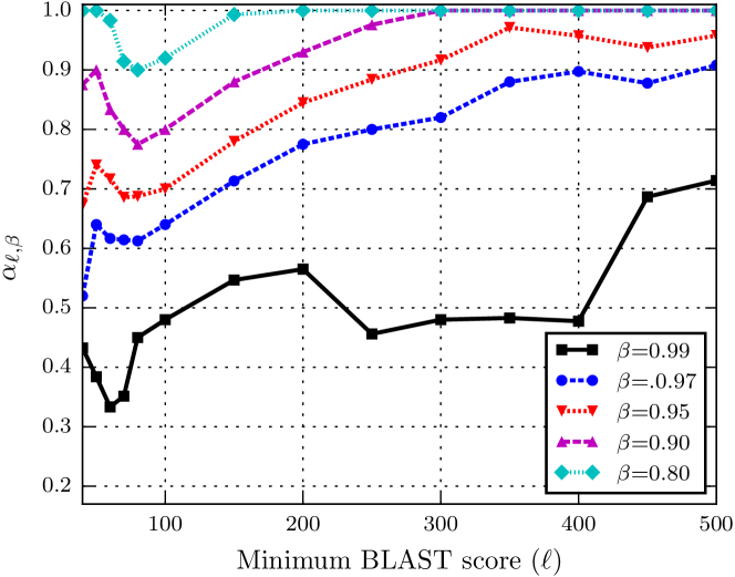
Figure 11: The transitivity of BLAST bit-score similarities for real proteins. The $\alpha_{\ell,\beta}$ measure is calculated for different values of $\ell$ and $\beta$.

The two main observations about (i) the relationship between sequence similarity and biological functions of protein couples, and (ii) the transitivity of BLAST bit-scores help us to design a heuristic algorithm for generating high-quality tuples (i.e., $\ell^{*}$-consistent tuples with value of $\ell^{*}$ very close to $\ell$) from sequence similarities.

5.2 Why Does MultiplePercolation Work?

The general class of PGM algorithms has been shown to be very powerful for global pairwise-network alignment problems. For example, PROPER is a state-of-the-art algorithm that uses PGM-based methods to align two networks Kazemi et al. (2016). There are several works on the theoretical and practical aspects of PGM algorithms Narayanan and Shmatikov (2009); Yartseva and Grossglauser (2013); Korula and Lattanzi (2014); Chiasserini et al. (2015a); Kazemi et al. (2015b); Kazemi (2016); Cullina and Kiyavash (2016); Cullina et al. (2016); Shirani et al. (2017, 2018); Dai et al. (2018); Mossel and Xu (2019). In this paper, we introduced a global MNA algorithm, as a new member of the PGM class. In this section, by using a parsimonious $k$-graph sampling model (as a generalization of the model from Kazemi et al. (2015b)), we prove that MultiplePercolation aligns all the nodes correctly if initially enough number of seed-tuples are provided. We first explain the model. Then we state the main theorem. Finally, we present experimental evaluations of MultiplePercolation over random graphs that are generated based on our $k$-graph sampling model.

5.2.1 A Multi-graph Sampling Model

Assume that all the $k$ networks $G_{i}(V_{i},E_{i})$ are evolved from an ancestor network $G(V,E)$ through node sampling (to model gene or protein deletion) and edge sampling (to model loss of protein-protein interactions) processes.

Definition 5 (The $Multi(G,\bm{t},\bm{s},k)$ sampling model).

Assume we have $\bm{t}=[t_{1},t_{2},\cdots,t_{k}]$ and $\bm{s}=[s_{1},s_{2},\cdots,s_{k}]$, $0<t_{i},s_{i}\leq 1$. The network $G_{i}(V_{i},E_{i})$ is sampled from $G(V,E)$ in the following way: First the nodes $V_{i}$ are sampled from $V$ independently with probability $t_{i}$; then the edges $E_{i}$ are sampled from those edges of graph $G$, whose both endpoints are sampled in $V_{i}$, by independent edge sampling processes with probability $s_{i}$. We define $t_{i,j}=\sqrt{t_{i}t_{j}}$ and $s_{i,j}=\sqrt{s_{i}s_{j}}$.

Definition 6 (A correctly matched tuple).

A tuple $T$ is a correctly matched tuple, if and only if all the nodes in $T$ are the same (say a node $u$), i.e., they are samples of a same node from the ancestor network $G$.

Definition 7 (A completely correctly matched tuple).

A correctly matched tuple $T$, which contains a different sample of a node $u$, is complete if and only if for all the vertex sets $V_{i},1\leq i\leq k$, if $u\in V_{i}$ then $V_{i}(T)=u$

Assume the $k$ networks $G_{i}(V_{i},E_{i})$ are sampled from a $G(n,p)$ random graph with $n$ nodes and average degrees of $np$. Now we state two main theorems that guarantee the performance of MultiplePercolation over the $Multi(G(n.p),\bm{t},\bm{s},k)$ sampling model. We first define two parameters $b_{t,s,r}$ and $a_{t,s,r}$:

$$b_{t,s,r}=\left[\dfrac{(r-1)!}{nt^{2}(ps^{2})^{r}}\right]^{\frac{1}{r-1}}\mbox{ and }a_{t,s,r}=(1-\dfrac{1}{r})b_{t,s,r}.$$ (2)

Theorem 8.

For $r\geq 2$ and an arbitrarily small but fixed $\tfrac{1}{6}>\epsilon>0$, assume that $n^{-1}\ll p\leq n^{-\frac{5}{6}-\epsilon}$. For an initial set of seed tuple $\mathcal{A}$, if $|\mathcal{A}_{i,j}|>(1+\epsilon)a_{t_{i,j},s_{i,j},r}$ for every $1\leq i,j\leq k,i\neq j$, then with high probability the MultiplePercolation algorithm percolates and for the final alignment $\pi$, we have $|\pi_{i,j}|=nt_{i,j}^{2}\pm o(n)$, where almost all the tuples are completely correctly matched tuples.

Theorem 9.

For $r\geq 2$ and an arbitrarily small but fixed $\tfrac{1}{6}>\epsilon>0$, assume that $n^{-1}\ll p\leq n^{-\frac{5}{6}-\epsilon}$. For an initial set of seed tuple $\mathcal{A}$, if for every $1\leq i\leq k$ there at least $c$ set of $\mathcal{A}_{i,j}$, $1\leq j\leq k$ and $i\neq j$, such that $|\mathcal{A}_{i,j}|>(1+\epsilon)a_{t_{i,j},s_{i,j},r}$, then with high probability the MultiplePercolation algorithm percolates and for the final alignment $\pi$, we have:

• Almost all the tuples $T\in\pi$ are correctly matched tuples.

• For a correctly matched tuple $T$, which contains the node $u$, if there are at least $k-c+1$ networks $G_{i}(V_{i},E_{1})$ such that $u\in V_{i}$, then $T$ is a completely correctly matched tuple

Note that Theorem 8 is the special case of Theorem 9 for $c=k-1$. The proofs of Theorems 8 and 9 follow from the generalization of the ideas that are used to prove (Kazemi et al., 2015a, Theorem 1 (Robustness of NoisySeeds)).

5.2.2 Experimental Results: Synthetic Networks

To evaluate the performance of our algorithm by using synthetic networks, we consider $k\in\{3,4,5\}$ randomly generated networks from the $Multi(G,\bm{t},\bm{s},k)$ model. In these experiments, we assume that a priori a set of seed-tuples $\mathcal{A}$ $(|\mathcal{A}|=a)$, with nodes from all the $k$ networks, are given and the MultiplePercolation algorithm starts the alignment process from these tuples.

In the first set of experiments, we assume $G$ is an Erdős-Rényi graph with $10^{5}$ nodes and an average degree of $20$. We assume $k$ networks $G_{i}$ are sampled from $G$ with node and edge sampling probabilities of $t=0.9$ and $s=0.9$, respectively. Figures 12, 13 and 14 show the simulation results for these experiments. We use $r=2$ for the MultiplePercolation algorithm. For each $k\in\{3,4,5\}$, the total number of correctly aligned tuples is provided. We observe that when there is enough number of tuples in the seed set, MultiplePercolation aligns correctly most of the nodes. We also see the sharp phase-transitions predicted in Theorems 8 and 9. According to Equation (2), we need $a_{t,s,r}=236$ correct seed-tuples to find the complete alignments for the model parameters of $n=10^{5},p=20/n,t=0.9$ and $s=0.9$. We observe that the phase transitions take place very close to $a_{t,s,r}=236$. For example, if $k=5$, in expectation there are $nt^{5}=59049$ nodes that are present in all the five networks. From Figures 12 (the black curve), it is clear that MultiplePercolation aligns correctly almost all these nodes. Also, in expectation, there are $\binom{5}{3}nt^{3}(1-t)^{2}=7290$ nodes that are present in exactly three networks. Again, from Figures 12 (the red curve), we observe that MultiplePercolation correctly aligns them.

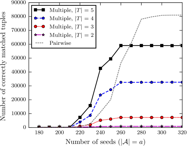
Figure 12: Multiple network alignment for graphs sampled from $Multi(G,\bm{t},\bm{s},k)$ with parameters $k=5,n=10^{5},p=20/n,t=0.9$ and $s=0.9$. We set $r=2$ for MultiplePercolation.

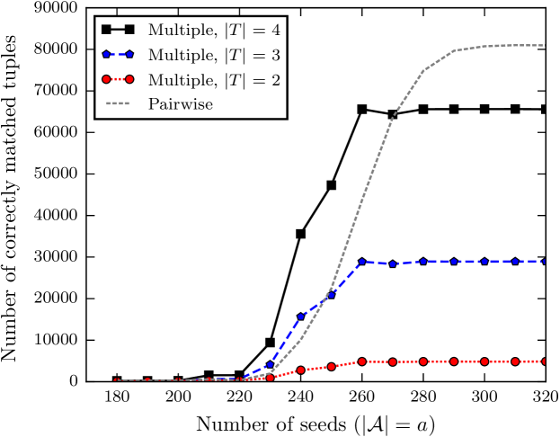
Figure 13: Multiple network alignment for graphs sampled from $Multi(G,\bm{t},\bm{s},k)$ with parameters $k=4,n=10^{5},p=20/n,t=0.9$ and $s=0.9$. We set $r=2$ for MultiplePercolation.

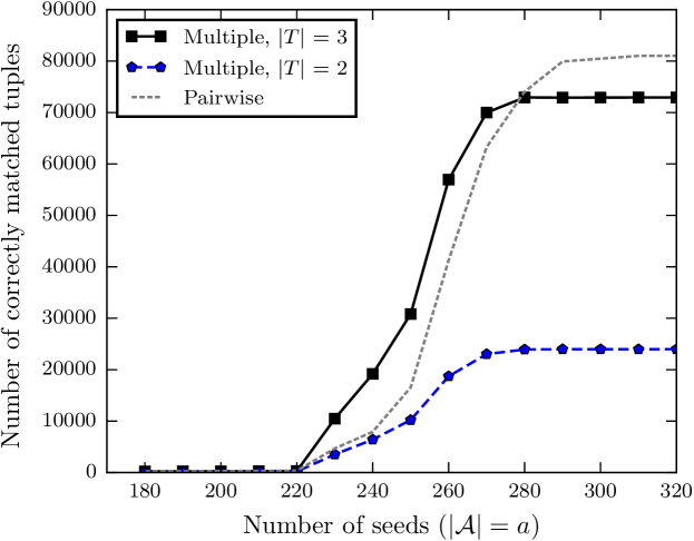
Figure 14: Multiple network alignment for graphs sampled from $Multi(G,\bm{t},\bm{s},k)$ with parameters $k=3,n=10^{5},p=20/n,t=0.9$ and $s=0.9$. We set $r=2$ for MultiplePercolation.

While we are only able to guarantee the performance of the MultiplePercolation algorithm for Erdős-Rényi graphs, we study the performance of our algorithms on two other network models with heavy-tailed degree distributions. For this reason, first, we apply the MultiplePercolation algorithm to a variant of power-law random graphs called the Chung-Lu model (CL) Chung and Lu (2002). In this model, the degree distribution of nodes follows a power law. Secondly, we apply MultiplePercolation to the Barabási Albert model (BA) Barabási and Albert (1999). This model generates random scale-free networks in a preferential attachment setting. In Figure 15, we observe that MultiplePercolation successfully aligns all the nodes from the $k=5$ networks correctly. We also observe that while for both models we need fewer number of seed than for Erdős-Rényi graphs, the required number of initial seeds for BA models is even less.

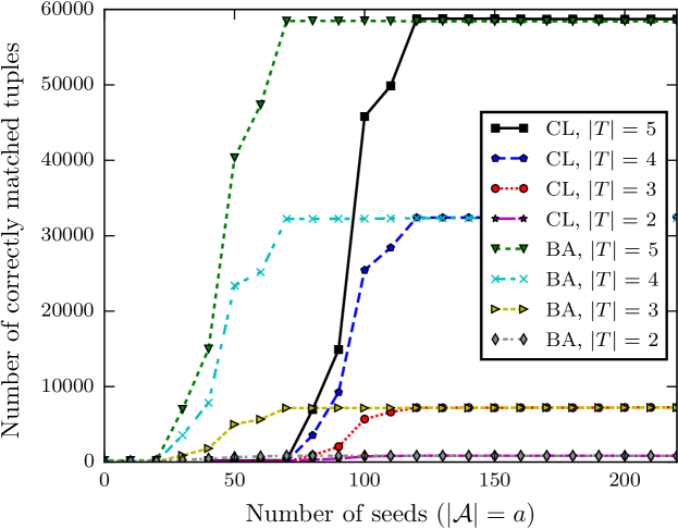
Figure 15: Multiple network alignment for graphs sampled from Chung-Lu (CL) and Barabási Albert (BA) models with $n=10^{5}$ nodes. The average degree of both graphs are 10. The node ($t$) and edge ($s$) sampling probabilities are both 0.9. We set $r=2$ for MultiplePercolation.

6 Conclusion

In this paper, we introduced a new one-to-one global multiple-network alignment algorithm, called MPGM. Our algorithm has two main steps. In the first step (SeedGeneration), it uses protein sequence-similarities to generate an initial seed-set of tuples. In the second step, MPGM applies a percolation-based graph-matching algorithm (called MultiplePercolation) to align the remaining unmatched proteins, by using only the structure of networks and the seed tuples from the first step. We have compared MPGM with several state-of-the-art methods. We observe that MPGM outperforms the other algorithms with respect to several measures. More specifically, MPGM finds many consistent tuples with high $d$-coverage (mainly for $d=k$). Also, it outputs alignments with a high structural similarity between networks, i.e., many interactions are conserved among aligned tuples. We have studied the transitivity of sequence similarities for real proteins and have found that it is reasonable to assume a pseudo-transitive relationship among them. We argue, based on this pseudo-transitivity property, that theSeedGeneration heuristic is able to find seed tuples with high functional similarities. In addition, we present a random-sampling model to generate $k$ correlated networks. By using this model, we prove conditions under which MultiplePercolation aligns (almost) all the nodes correctly if initially enough seed tuples are provided.

Acknowledgements.

The work of Ehsan Kazemi was supported by Swiss National Science Foundation (Early Postdoc.Mobility) under grant number 168574.

Appendix A Table of Notations

Table 5:

$G_{i}(V_{i},E_{i})$	A network with vertex set $V_{i}$ and edge set $E_{i}$.
$(u,v)$	An edge between nodes $u$ and $v$.
$N_{i}(u)$	The set of neighbors of node $u$ in $G_{i}$.
$BlastBit(u,v)$	BLAST bit-score similarity of two proteins $u$ and $v$
$[u,v]$	A couple of proteins $u$ and $v$.
$T$	A tuple.
$\mathcal{A}$	Initial seed-tuples.
$\pi$	The final alignment.
$|T|$	Number of nodes in tuple $T$.
$V(T)$	The set of networks such that have a node in the tuple $T$.
$V(u)$	The network $V_{i}$ such that $u\in V_{i}$.
$\mathcal{S}_{\geq\ell}$	The set of all couples with BLAST bit-score similarities at least $\ell$.
$\mathcal{A}(u)$	Returns the tuple $T\in\mathcal{A}$ such that $u\in T$. If there is no such tuple, we define $\mathcal{A}(u)=\emptyset$.
$E_{T_{i},T_{j}}$	The set of all the interactions between nodes from the two tuples $T_{i}$ and $T_{j}$, i.e., $E_{T_{i},T_{j}}=\{e=(u,v)|u\in T_{i},v\in T_{j}\}$.
$V(E_{T_{i},T_{j}})$	The set of networks such that have an edge in $E_{T_{i},T_{j}}$.
$C(\pi)$	The set of consistent tuples in an alignment $\pi$.

Appendix B Detailed Comparisons

Tables 6, 7, 8 and 9 provide detailed comparisons for tuples with different coverages. Table 6 compares algorithms over tuples with nodes from five networks. The second step of MPGM (i.e., MultiplePercolation) uses PPI networks to generate 3076 tuples out of initial seed-tuples. We observe that MPGM (for $\ell=40$) finds an alignment with the maximum $d$-coverage, $\#CC_{5}$, $\#CP_{5}$ and $SS_{p}(\pi)$. In addition, the first step of MPGM (i.e., SeedGeneration) has the best performance on $Spec_{5}$, $\overline{SS_{p}}(\pi)$ and MNE. This was expected, because MultiplePercolation uses only network structure, a less reliable source of information for functional similarity in comparison to sequence similarities, to align new nodes. From this table, it is clear that MPGM outperforms the other algorithms with respect to all the measures.

Table 6: Comparison results for tuples of size five. For MPGM we set $r=1$.

	SeedGeneration ($\ell$)			MPGM ($\ell$)			F	B	S	C	I	M	G
	40	80	150	40	80	150
$d$-coverage	1366	880	568	3076	3062	3068	2233	867	1132	1104	379	1896	1942
$\#CC_{5}$	386	248	159	707	647	541	449	187	209	200	23	312	25
$\#CP_{5}$	1930	1240	795	3535	3235	2705	2245	1082	1279	1234	126	1560	125
$Spec_{5}$	0.291	0.286	0.284	0.244	0.222	0.184	0.21	0.22	0.187	0.185	0.063	0.194	0.013
$SS_{p}(\pi)$	5294	3519	2251	10659	10002	9285	7078	2788	3315	3097	554	5279	2614
$\overline{SS_{p}}(\pi)$	3.928	4.018	3.993	3.55	3.326	3.074	3.22	3.239	2.944	2.818	1.482	3.071	1.37
MNE	2.927	2.943	3.049	3.008	3.071	3.144	3.014	3.162	3.312	3.071	3.469	3.185	3.889

Table 7: Comparison results for tuples of size four. For MPGM we set $r=1$.

	SeedGeneration ($\ell$)			MPGM ($\ell$)			F	B	S	C	I	M	G
	40	80	150	40	80	150
$d$-coverage	1933	1591	1133	2719	2520	2321	3527	1663	1547	1670	1475	3305	4168
$\#CC_{4}$	580	532	392	631	534	435	834	510	414	474	118	652	215
$\#CP_{4}$	2320	2128	1568	2524	2136	1740	3336	2398	1903	2272	560	2608	860
$Spec_{4}$	0.339	0.366	0.369	0.277	0.256	0.224	0.299	0.329	0.291	0.306	0.092	0.297	0.075
$SS_{p}(\pi)$	8309	7335	5465	10449	9087	7902	12829	7043	5863	6522	2953	12840	7988
$\overline{SS_{p}}(\pi)$	4.591	4.814	4.982	4.213	3.984	3.726	4.095	4.34	3.922	4.044	2.156	3.951	1.947
MNE	2.565	2.648	2.717	2.571	2.621	2.668	2.597	2.733	2.664	2.73	3.168	2.720	3.525

Table 8: Comparison results for tuples of size three. For MPGM we set $r=1$.

	SeedGeneration ($\ell$)			MPGM ($\ell$)			F	B	S	C	I	M	G
	40	80	150	40	80	150
$d$-coverage	2342	2227	1842	2502	2522	2523	2180	2320	1951	1981	2869	2736	2157
$\#CC_{3}$	775	794	692	603	598	545	472	801	617	662	308	620	232
$\#CP_{3}$	2325	2382	2076	1809	1794	1635	1416	2886	2132	2352	1027	1860	696
$Spec_{3}$	0.462	0.486	0.500	0.384	0.382	0.349	0.35	0.437	0.417	0.436	0.153	0.397	0.134
$SS_{p}(\pi)$	11509	11672	9988	10040	10070	9430	8197	11509	9064	9526	7463	14530	6092
$\overline{SS_{p}}(\pi)$	6.007	6.319	6.394	5.263	5.348	4.995	4.956	5.706	5.441	5.587	3.224	5.389	2.884
MNE	2.239	2.290	2.372	2.312	2.336	2.35	2.348	2.276	2.31	2.264	2.83	2.431	3.022

Table 9: Comparison results for tuples of size two. For MPGM we set $r=1$.

	SeedGeneration ($\ell$)			MPGM ($\ell$)			F	B	S	C	I	M	G
	40	80	150	40	80	150
$d$-coverage	3510	4013	4411	3402	3675	3825	3118	3265	2820	2988	5620	3958	2110
$\#CC_{2}$	859	1088	1357	579	645	703	495	900	702	905	541	685	202
$\#CP_{2}$	1718	2176	2714	1158	1290	1406	990	2309	1644	2073	1224	1370	404
$Spec_{2}$	0.611	0.619	0.646	0.527	0.519	0.529	0.462	0.557	0.558	0.618	0.231	0.495	0.229
$SS_{p}(\pi)$	15049	18777	22849	10664	12032	12918	9035	14749	12003	14898	12853	22048	7897
$\overline{SS_{p}}(\pi)$	8.157	8.286	8.551	7.025	7.153	7.161	6.118	7.375	7.378	8.124	4.21	5.729	3.826
MNE	1.946	1.944	1.968	2.01	2.03	2.002	2.163	1.987	1.951	1.987	2.464	2.152	2.797

Appendix C BLAST Bit-score Similarities and GO terms

To provide experimental evidence for our hypothesis, we look at the biological similarity of protein couples versus their BLAST bit-score similarities. For this reason, we define a gene-ontology consistency (GOC) measure (based on the measure introduced in Mistry and Pavlidis [2008]) to evaluate the relationship between BLAST bit-scores and the experimentally verified GO terms. This measure represents the percentage of pairs of proteins with BLAST bit-score similarity of at least $\ell$, such that they share at least one GO term. Formally, we define

$$goc_{\geq\ell}=$$

$$\dfrac{|\{[p_{i},p_{j}]|BLAST(p_{i},p_{j})\geq\ell\text{ and }go(p_{i})\cap go(p_{j})\neq\emptyset\}|}{|\{[p_{i},p_{j}]|BLAST(p_{i},p_{j})\geq\ell,go(p_{i})\neq\emptyset\text{ and }go(p_{j})\neq\emptyset\}|}.$$ (3)

In this section, we consider only experimentally verified GO terms. Figure 16 shows the $goc_{\geq\ell}$ measure for couples of proteins among five eukaryotic species, namely C. elegans (ce), D. melanogaster (dm), H. sapiens (hs), M. musculus (mm) and S. cerevisiae (sc). In this figure, the results are provided for cases, where we consider (i) all the experimental GO terms, (ii) cellular component (CC) annotations, (iii) molecular function (MF) annotations, and (iv) biological process (BP) annotations. For further experiments, we look at the average of semantic similarity $SS_{p}$ (section 3) between couples of proteins with BLAST bit-score similarity of at least $\ell$. Figure 17 shows the $SS_{p}$ for couples of proteins with BLAST bit-score similarities of at least $\ell$. We observe that, for couples of proteins with higher BLAST bit-score similarities, the average of $SS_{p}$ measure increases.

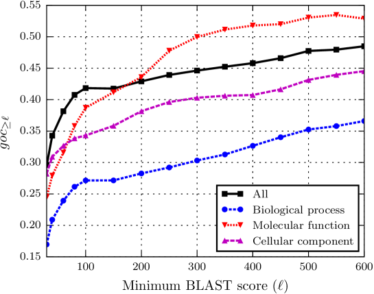
Figure 16: The $goc_{\geq\ell}$ measure for couples of proteins with BLAST bit-score similarities of at least $\ell$.

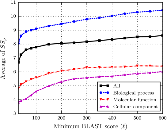
Figure 17: Average of $SS_{p}$ for couples of proteins with BLAST bit-score similarities of at least $\ell$. We observe that, for couples of proteins with higher BLAST bit-score similarities, the average of $SS_{p}$ measure increases.

Appendix D GO Annotation: Statistics

In this appendix, we look at a few statistics regarding GO annotations. GO annotations comprises three orthogonal taxonomies for a gene product: molecular-function, biological-process and cellular-component. This information is captured in three different directed acyclic graphs (DAGs). The roots (the most general annotations for each category) of these DAGs are:

• GO:0003674 for molecular function annotations

• GO:0008150 for biological process annotations

• GO:0005575 for cellular component annotations

For information content of each GO term, we use the SWISS-PROT-Human proteins, and counted the number of times each concept occurs. Information content is calculated based on the following information:

• Number of GO terms in the dataset is 26831.

• Number of annotated proteins in the dataset is 38264085.

• Number of experimental GO terms in the dataset is 24017.

• Number of experimentally annotated proteins in the dataset is 102499.

Table 10 provides information related to different categories of GO annotations for the five networks we used in our experiments.

Table 10: Statistics for experimental GO annotations.

GO type	$\#$GO	$\#$proteins	Avg. $\#$GO
All	20738	28896	49.47
Biological process	14876	20723	48.21
Molecular function	3938	21670	7.84
Cellular component	1924	21099	12.35

Next we report the number of experimentally annotated proteins (at the cut-off level 5 of DAGs) in each network:

• C. elegans: 1544 out of 4950 proteins (31.2 %).

• D. melanogaster: 4653 out of 8532 proteins (54.5 %).

• H. sapiens: 10929 out of 19141 proteins (57.1 %).

• M. musculus: 7150 out of 10765 proteins (66.4 %).

• S. cerevisiae: 4819 out of 6283 proteins (76.7 %).

The probabilities of sharing at least one GO term (at the cut-off level 5) for tuples of size two to five, when all the proteins of a tuple are annotated, are as follows:

• tuples of size 2: 0.215

• tuples of size 3: 0.042

• tuples of size 4: 0.009

• tuples of size 5: 0.002

Also, the probabilities of sharing at least one GO term (at the cut-off level 5) for tuples of size two to five, when at least two proteins from each tuple are annotated, are as follows:

• tuples of size 2: 0.215

• tuples of size 3: 0.167

• tuples of size 4: 0.120

• tuples of size 5: 0.081

In Figure 18, the total number of annotated proteins, at different cut-off levels, are shown. Also, the number of GO terms and the average number of GO terms for each annotated protein, at different cut-off levels, are shown in Figures 19 and 20, receptively.

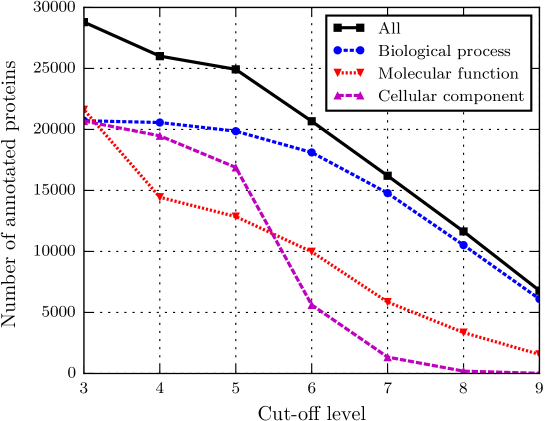
Figure 18: Number of annotated proteins for different cut-off levels

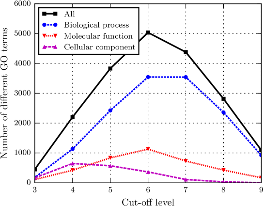
Figure 19: Number of different GO terms for different cut-off levels

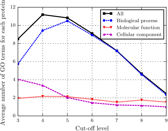
Figure 20: Average number of GO terms for each annotated protein for different cut-off levels

References

- Ahmet Emre Aladag and Cesim Erten [2013] Ahmet Emre Aladag and Cesim Erten. Spinal: scalable protein interaction network alignment. Bioinformatics, 29(7):917–924, 2013.
- Alkan and Erten [2014] Ferhat Alkan and Cesim Erten. Beams: backbone extraction and merge strategy for the global many-to-many alignment of multiple ppi networks. Bioinformatics, 30(4):531–539, 2014.
- Altschul et al. [1990] Stephen F Altschul, Warren Gish, Webb Miller, Eugene W Myers, and David J Lipman. Basic local alignment search tool. Journal of Molecular Biology, 215(3):403–410, 1990.
- Apweiler et al. [2004] Rolf Apweiler, Amos Bairoch, Cathy H Wu, Brigitte Barker, Winona Cand Boeckmann, Serenella Ferro, Elisabeth Gasteiger, Hongzhan Huang, Rodrigo Lopez, Michele Magrane, et al. UniProt: the universal protein knowledgebase. Nucleic Acids Research, 32(suppl 1):D115–D119, 2004.
- Barabási and Albert [1999] Albert-László Barabási and Réka Albert. Emergence of scaling in random networks. science, 286(5439):509–512, 1999.
- Chiasserini et al. [2015a] Carla F. Chiasserini, Michele Garetto, and Emilio Leonardi. De-anonymizing scale-free social networks by percolation graph matching. In Proc. of IEEE INFOCOM 2015, Hong Kong, April 2015a.
- Chiasserini et al. [2015b] Carla F. Chiasserini, Michele Garetto, and Emilio Leonardi. Impact of Clustering on the Performance of Network De-anonymization. In Proc. of ACM COSN 2015, Palo Alto, CA, USA, November 2015b.
- Chung and Lu [2002] Fan Chung and Linyuan Lu. Connected components in random graphs with given expected degree sequences. Annals of combinatorics, 6(2):125–145, 2002.
- Cullina and Kiyavash [2016] Daniel Cullina and Negar Kiyavash. Improved Achievability and Converse Bounds for Erdős–Rényi Graph Matching. In Proceedings of the 2016 ACM SIGMETRICS International Conference on Measurement and Modeling of Computer Science, New York, NY, USA, 2016. ACM.
- Cullina et al. [2016] Daniel Cullina, Kushagra Singhal, Negar Kiyavash, and Prateek Mittal. On the Simultaneous Preservation of Privacy and Community Structure in Anonymized Networks. arXiv e-prints, art. arXiv:1603.08028, Mar 2016.
- Dai et al. [2018] Osman Emre Dai, Daniel Cullina, Negar Kiyavash, and Matthias Grossglauser. On the Performance of a Canonical Labeling for Matching Correlated Erdos-Renyi Graphs. arXiv e-prints, art. arXiv:1804.09758, Apr 2018.
- Dean and Ghemawat [2008] Jeffrey Dean and Sanjay Ghemawat. Mapreduce: simplified data processing on large clusters. Communications of the ACM, 51(1):107–113, 2008.
- Flannick et al. [2006] Jason Flannick, Antal Novak, Balaji S Srinivasan, Harley H McAdams, and Serafim Batzoglou. Graemlin: general and robust alignment of multiple large interaction networks. Genome research, 16(9):1169–1181, 2006.
- Gligorijević et al. [2015] Vladimir Gligorijević, Noël Malod-Dognin, and Nataša Pržulj. Fuse: multiple network alignment via data fusion. Bioinformatics, 2015.
- Hashemifar and Xu [2014] Somaye Hashemifar and Jinbo Xu. HubAlign: an accurate and efficient method for global alignment of protein–protein interaction networks. Bioinformatics, 30(17):i438–i444, 2014.
- Hermjakob et al. [2004] Henning Hermjakob, Luisa Montecchi-Palazzi, Chris Lewington, Sugath Mudali, Samuel Kerrien, Sandra Orchard, Martin Vingron, Bernd Roechert, Peter Roepstorff, Alfonso Valencia, et al. IntAct: an open source molecular interaction database. Nucleic Acids Research, 32(suppl 1):D452–D455, 2004.
- Hu et al. [2014] Jialu Hu, Birte Kehr, and Knut Reinert. NetCoffee: a fast and accurate global alignment approach to identify functionally conserved proteins in multiple networks. Bioinformatics, 30(4):540–548, 2014.
- Ibragimov et al. [2014] Rashid Ibragimov, Maximilian Malek, Jan Baumbach, and Jiong Guo. Multiple graph edit distance: simultaneous topological alignment of multiple protein-protein interaction networks with an evolutionary algorithm. In Proceedings of the 2014 Annual Conference on Genetic and Evolutionary Computation. ACM, 2014.
- Jeong and Yoon [2015] Hyundoo Jeong and Byung-Jun Yoon. Accurate multiple network alignment through context-sensitive random walk. BMC systems biology, 9(Suppl 1):S7, 2015.
- Kalaev et al. [2008] Maxim Kalaev, Mike Smoot, Trey Ideker, and Roded Sharan. Networkblast: comparative analysis of protein networks. Bioinformatics, 24(4), 2008.
- Kazemi [2016] Ehsan Kazemi. Network alignment: Theory, algorithms, and applications. PhD dissertation, EPFL, 2016.
- Kazemi and Grossglauser [2016] Ehsan Kazemi and Matthias Grossglauser. On the Structure and Efficient Computation of IsoRank Node Similarities. arXiv e-prints, art. arXiv:1602.00668, Feb 2016.
- Kazemi et al. [2015a] Ehsan Kazemi, S. Hamed Hassani, and Matthias Grossglauser. Growing a Graph Matching from a Handful of Seeds. Proc. of the VLDB Endowment, 8(10):1010–1021, 2015a.
- Kazemi et al. [2015b] Ehsan Kazemi, Lyudmila Yartseva, and Matthias Grossglauser. When Can Two Unlabeled Networks Be Aligned Under Partial Overlap? In Allerton, Monticello, IL, USA, October 2015b.
- Kazemi et al. [2016] Ehsan Kazemi, Hamed Hassani, Matthias Grossglauser, and Hassan Pezeshgi Modarres. PROPER: global protein interaction network alignment through percolation matching. BMC Bioinformatics, 17(1):527, 2016.
- Korula and Lattanzi [2014] Nitish Korula and Silvio Lattanzi. An efficient reconciliation algorithm for social networks. Proc. of the VLDB Endowment, 7(5):377–388, 2014.
- Kuchaiev et al. [2010] Oleksii Kuchaiev, Tijana Milenković, Vesna Memišević, Wayne Hayes, and Nataša Pržulj. Topological network alignment uncovers biological function and phylogeny. Journal of the Royal Society Interface, pages 1341–1354, 2010.
- Liao et al. [2009] Chung-Shou Liao, Kanghao Lu, Michael Baym, Rohit Singh, and Bonnie Berger. IsoRankN: spectral methods for global alignment of multiple protein networks. Bioinformatics, 25(12):i253–i258, 2009.
- Lord et al. [2003] Phillip W. Lord, Robert D. Stevens, Andy Brass, and Carole A. Goble. Investigating semantic similarity measures across the gene ontology: the relationship between sequence and annotation. Bioinformatics, 19(10):1275–1283, 2003.
- Malod-Dognin and Pržulj [2015] Noël Malod-Dognin and Nataša Pržulj. L-GRAAL: Lagrangian graphlet-based network aligner. Bioinformatics, 31(13):2182–2189, 2015.
- Meng et al. [2016] Lei Meng, Aaron Striegel, and Tijana Milenković. Local versus global biological network alignment. Bioinformatics, 2016.
- Mistry and Pavlidis [2008] Meeta Mistry and Paul Pavlidis. Gene ontology term overlap as a measure of gene functional similarity. BMC bioinformatics, 9(1):327, 2008.
- Mossel and Xu [2019] Elchanan Mossel and Jiaming Xu. Seeded Graph Matching via Large Neighborhood Statistics. In Proceedings of the Thirtieth Annual ACM-SIAM Symposium on Discrete Algorithms, SODA, pages 1005–1014, 2019.
- Narayanan and Shmatikov [2009] Arvind Narayanan and Vitaly Shmatikov. De-anonymizing social networks. In Proc. of IEEE Symposium on Security and Privacy 2009, Oakland, CA, USA, May 2009.
- Neyshabur et al. [2013] Behnam Neyshabur, Ahmadreza Khadem, Somaye Hashemifar, and Seyed Shahriar Arab. NETAL: a new graph-based method for global alignment of protein–protein interaction networks. Bioinformatics, 29(13):1654–1662, 2013.
- Notredame et al. [2000] Cédric Notredame, Desmond G Higgins, and Jaap Heringa. T-coffee: A novel method for fast and accurate multiple sequence alignment. Journal of molecular biology, 302(1):205–217, 2000.
- Patro and Kingsford [2012] Rob Patro and Carl Kingsford. Global network alignment using multiscale spectral signatures. Bioinformatics, 28(23):3105–3114, 2012.
- Radu and Charleston [2015] Alex Radu and Michael Charleston. Node handprinting: a scalable and accurate algorithm for aligning multiple biological networks. Journal of Computational Biology, 22(7):687–697, 2015.
- Resnik [1999] Philip Resnik. Semantic similarity in a taxonomy: An information-based measure and its application to problems of ambiguity in natural language. Journal of artificial intelligence research, 11:95–130, 1999.
- Sahraeian and Yoon [2013] Sayed Mohammad Ebrahim Sahraeian and Byung-Jun Yoon. SMETANA: accurate and scalable algorithm for probabilistic alignment of large-scale biological networks. PLoS One, 8(7):e67995, 2013.
- Saraph and Milenković [2014] Vikram Saraph and Tijana Milenković. Magna: Maximizing accuracy in global network alignment. Bioinformatics, 30(20):2931–2940, 2014.
- Schlicker and Albrecht [2008] Andreas Schlicker and Mario Albrecht. Funsimmat: a comprehensive functional similarity database. Nucleic acids research, 36(suppl 1):D434–D439, 2008.
- Sharan et al. [2005] Roded Sharan, Silpa Suthram, Ryan M. Kelley, Tanja Kuhn, Scott McCuine, Peter Uetz, Taylor Sittler, Richard M. Karp, and Trey Ideker. Conserved patterns of protein interaction in multiple species. Proceedings of the National Academy of Sciences of the United States of America, 102(6):1974–1979, 2005.
- Shirani et al. [2017] Farhad Shirani, Siddharth Garg, and Elza Erkip. Seeded graph matching: Efficient algorithms and theoretical guarantees. In Asilomar Conference on Signals, Systems, and Computers, ACSSC, pages 253–257, 2017.
- Shirani et al. [2018] Farhad Shirani, Siddharth Garg, and Elza Erkip. Typicality Matching for Pairs of Correlated Graphs. In 2018 IEEE International Symposium on Information Theory, ISIT, pages 221–225, 2018.
- Singh et al. [2007] Rohit Singh, Jinbo Xu, and Bonnie Berger. Pairwise Global Alignment of Protein Interaction Networks by Matching Neighborhood Topology. In Proc. of Research in Computational Molecular Biology 2007, San Francisco, CA, USA, April 2007.
- Vijayan and Milenkovic [2018] Vipin Vijayan and Tijana Milenkovic. Multiple network alignment via multimagna++. IEEE/ACM Trans. Comput. Biology Bioinform., 15(5):1669–1682, 2018.
- Vijayan et al. [2015] Vipin Vijayan, Vikram Saraph, and Tijana Milenković. MAGNA++: Maximizing Accuracy in Global Network Alignment via both node and edge conservation. Bioinformatics, 31(14):2409–2411, 2015.
- Yartseva and Grossglauser [2013] Lyudmila Yartseva and Matthias Grossglauser. On the performance of percolation graph matching. In Proc. of ACM COSN 2013, Boston, MA, USA, October 2013.