Extended Vertical Lists for Temporal Pattern Mining
from Multivariate Time Series

Abstract

Temporal Pattern Mining (TPM) is the problem of mining predictive complex temporal patterns from multivariate time series in a supervised setting. We develop a new method called the Fast Temporal Pattern Mining with Extended Vertical Lists. This method utilizes an extension of the Apriori property which requires a more complex pattern to appear within records only at places where all of its subpatterns are detected as well. The approach is based on a novel data structure called the Extended Vertical List that tracks positions of the first state of the pattern inside records. Extensive computational results indicate that the new method performs significantly faster than the previous version of the algorithm for TMP. However, the speed-up comes at the expense of memory usage.

1 Introduction

Continuously expanding resources for computing, data storage, and transmission have been enabling analyses of complex data sets emerging from various domains such as medical event detection and prediction [1, 2, 3, 4], fraud detection [5], etc. We consider the problem of extracting temporal patterns from multivariate time series records in a supervised setting. Our main contribution is a faster algorithm for mining class-specific patterns having temporal relations between their states. Our motivation is to develop an algorithm that can be built into a workflow for real-time analytic engines. The framework for frequent pattern mining was developed in [6, 7]. Several extensions have been introduced [1, 2, 3, 4] which were successfully utilized in medical decision-making [8, 9, 10, 11]. Data is collected in the form of a set of records where each record is characterized by numerical (e.g., heart rate or blood pressure) and categorical (e.g., an indicator of whether a patient is on medication or not) time series combined with categorical and numerical attributes like gender, age, etc.

In this paper, the work of Batal et al. [10] is extended by introducing a new algorithm called the Fast Temporal Pattern Mining with Extended Vertical Lists. The idea is to utilize the Apriori [12] property on the level of pattern positions inside records. Informally, we require the Apriori property to state that a Temporal Pattern (TP) may appear only in the records where all of its subpatterns appear as well. For example, if TP “Heart Rate is Very High before Blood Pressure is Low” is found in record $i$, then both its subpatterns “Heart Rate is Very high” and “Blood Pressure is Low” must appear in record $i$. In this form, the Apriory property was used to reduce the search space for mining TPs [10] and similar notions as itemsets [13] and sequential patterns [2, 14] via the vertical data format [13]. We suggest a new data structure called the Extended Vertical List that keeps track of positions of the first state of the TP inside the records and links them to the positions of the pattern parent (a subpattern without the first state) inside the records. This idea allows us to reduce the computational time by a factor of several hundreds on a number of datasets (see Section 4 for details). The speed-up comes at the cost of increased memory consumption, which is a typical trade-off in such a kind of algorithms.

2 Concepts and Definitions

Assume dataset $D$ of $n$ records $d_{i},\leavevmode\nobreak\ i=1,\dots,n$, where each record is composed of $m$ time series $x_{j}^{i}\in X_{j}$ and an outcome, or class label, $y_{i}\in Y$ associated with it: $d_{i}=\left(x_{1}^{i},x_{2}^{i},\dots,x_{m}^{i},y_{i}\right).$ The overall goal is to train classifier $f:X_{1}\times\dots\times X_{m}\rightarrow Y$, i.e., we consider the Supervised Multiple Time Series Classification Problem. In such problems, time series are typically mapped first into a feature domain with feature extraction techniques: $g:X_{1}\times\dots\times X_{m}\rightarrow F_{1}\times\dots\times F_{k}$. In this paper, we focus on improving computational aspects of function $g$. In this section, we follow the definitions given in [10] with slight modifications for the presentation to be self-contained.

We start with reducing dimensionality through converting each time series into a set of temporal abstractions in the form

$$\left<(V_{1},s_{1},e_{1}),\dots,(V_{k},s_{k},e_{k})\right>,$$

where $V_{i}\in\Sigma$ is a temporal abstraction that is in effect from start time $s_{i}$ till end time $e_{i}$, e.g., temporal abstraction (“Low”,5,12) means that the time series was low from time 5 till time 12; $\Sigma$ is the alphabet, or set of possible abstractions (e.g., $\Sigma=\{\text{``Low'', ``Normal'', ``High''}\}$). For a given set of temporal abstractions, we also require $s_{1}\leq e_{1}\leq s_{2}\dots\leq s_{k}\leq e_{k}$, meaning that no abstraction can start earlier than any previous one finishes.

The alphabet $\Sigma$ can be defined in several ways. In this paper, we focus on value and trend abstractions; particular examples include:

1. Value Abstractions: $\Sigma=\{\downarrow\downarrow,\downarrow,\textendash,\uparrow,\uparrow\uparrow\}$ where $\downarrow\downarrow$, $\downarrow$, $\textendash$, $\uparrow$, and $\uparrow\uparrow$ stand for “Very Low”, “Low”, “Normal”, “High” and “Very High”, respectfully. Exact ranges for transformation may be set up by a field expert. In our computations, we used time-series-specific percentiles $\{0.1,0.25,0.75,0.9\}$.

2. Trend Abstractions. $\Sigma=\{\rightarrow,\nearrow,\searrow\}$ where $\rightarrow$, $\nearrow$, and $\searrow$ stand for “Steady”, “Increasing”, and “Decreasing”, respectfully. For this transformation, we used the approach by [15].

Now we are ready to define the Multivariate State Sequence which is a representation of the corresponding multivariate time series in alphabet $\Sigma$.

Definition 1

• $S=(F,V)$ is a state where is $F$ is a variable label and $V\in\Sigma$ is an abstraction value.

• $E=(F,V,s,e)$ is a state interval where $(F,V)$ is a state and $s$ and $e$ are the start and end times of the state interval.

• $Z=\langle E_{1},\dots,E_{l}\rangle$ is a Multivariate State Sequence (MSS) with the states sorted according to the non-decreasing order of their start times: $E_{i}.s\leq E_{i+1}.s,1\leq i\leq l-1$.

Example 1

$S=(\text{HR},\downarrow)$ is a state indicating that temporal variable Heart Rate is on a low level, while state interval $E=(\text{HR},\downarrow,12,15)$ extends the state by including information on its start and end time moments. Finally, an MSS combines several state intervals coming from different time series as in MSS $Z=\langle E_{1}=(\text{HR},\textendash,0,3)$, $E_{2}=(\text{BP},\downarrow,1,9)$, $E_{3}=(\text{HR},\downarrow,4,7)$, $E_{4}=(\text{HR},\textendash,8,11)$, $E_{5}=(\text{BP},\textendash,10,17)$, $E_{6}=(\text{HR},\downarrow,12,14)$, $E_{7}=(\text{HR},\downarrow\downarrow,15,19)$, $E_{8}=(\text{BP},\downarrow,18,22)$, $E_{9}=(\text{HR},\downarrow,20,29)$, $E_{10}=(\text{BP},\uparrow\uparrow,23,26)$, $E_{11}=(\text{BP},\downarrow,27,31)$, $E_{12}=(\text{HR},\textendash,30,38)$, $E_{13}=(\text{BP},\textendash,32,36)\rangle$ (see Figure1).

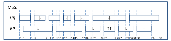
Figure 1: An example of an MSS with time variables Heart Rate (HR) and Blood Pressure (BP).

Temporal Pattern is the next level of abstraction, which allows to remove exact values of start and end times and focus on temporal relationships of the state intervals. For this purpose, Allen’s logic is often used [16], where only two time relations out of 13 possible are chosen (see [10] for a relevant discussion).

For two state intervals $E_{i}$ and $E_{j}$ with $E_{i}.s\leq E_{j}.s$, we say that $E_{i}$ finishes before $E_{j}$ if $E_{i}.e<E_{j}.s$ and denote it as $R(E_{i},E_{j})=b$. Otherwise, we say that $E_{i}$ co-occurs with $E_{j}$ and denote it as $R(E_{i},E_{j})=c$.

Definition 2

• $P=\left(\langle S_{1},\dots,S_{k}\rangle,R\right)$ is a Temporal Pattern (TP) of size $k$ $(|P|=k)$ with states $S_{1},\dots,S_{k}$, where $R$ is a (upper-triangular) matrix describing pair-wise temporal relationships between the states: $R_{i,j}\in\{b,c\},\leavevmode\nobreak\ 1\leq i<j\leq k$.

• Given MSS $Z=\left<E_{1},E_{2},\dots,E_{l}\right>$ and temporal pattern $P=(\left<S_{1},\dots,S_{k}\right>,R)$ $(k\leq l)$, we say that $Z$ contains $P$, denoted as $P\in Z$, if there is a mapping $\pi:\{1,\dots,k\}\to\{1,\dots,l\}$ that matches every state $S_{i}$ in $P$ to a state interval $E_{\pi(i)}$ in $Z$ such that:

  1. $S_{i}.F=E_{\pi(i)}.F\leavevmode\nobreak\ \text{and}\leavevmode\nobreak\ S_{i}.V=E_{\pi(i)}.V,\leavevmode\nobreak\ 1\leq i\leq k$,

  2. $\pi(i)<\pi(j),\leavevmode\nobreak\ i<j$,

  3. $R(E_{\pi(i)},E_{\pi(j)})=R_{i,j},\leavevmode\nobreak\ i<j$.

The first requirement guarantees that each state of $P$ matches an appropriate state interval in $Z$, while the rest of the constrains enforce that the temporal relations in $P$ correspond to a correct overlapping of the state intervals in $Z$.

Example 2

$P=\left(\langle S_{1},S_{2},S_{3}\rangle,R\right)$ is a TP of size $3$ (see Figure 2(b)) with states $S_{1}=(\text{HR},\textendash)$, $S_{2}=(\text{BP},\textendash)$, $S_{3}=(\text{HR},\downarrow)$ and relationships matrix $R=\left(R_{1,2},R_{1,3},R_{2,3}\right)$, where $R_{1,2}=c$, $R_{1,3}=b$, and $R_{2,3}=c$. The MSS from Figure 1 contains this TP since MSS’s state intervals $E_{4}=(\text{HR},\textendash,8,11)$, $E_{5}=(\text{BP},\textendash,10,17)$, and $E_{6}=(\text{HR},\downarrow,12,14)$ match the states of $P$ and the time relationships are satisfied: for example, $E_{4}.e=11>10=E_{5}.s$ and, therefore, state intervals 4 and 5 co-occur, or $R(E_{4},E_{5})=c$, and equals the specified time relationship $R_{1,2}$ between states 1 and 2 of $P$.

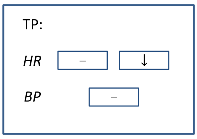
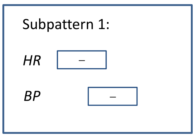
(a)

(b)

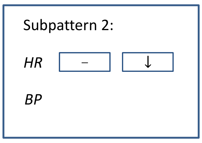
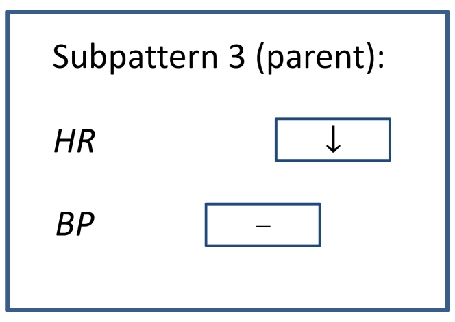
(c)

(d)

Figure 2: TP and its subpatterns: (a) an example of a TP; (b) the subpattern without the last state; (c) the subpattern without the middle state; (d) the parent, the subpattern without the first state.

Definition 3

$\widetilde{P}$, $|\widetilde{P}|=\widetilde{k}$, is a subpattern of $P$, $|P|=k$ ($\widetilde{k}\leq k$), denoted as $\widetilde{P}\subset P$, if there is a mapping $\pi:\{1,\dots,\widetilde{k}\}\to\{1,\dots,k\}$ such that:

1. $\widetilde{S}_{i}=S_{\pi(i)},1\leq i\leq\widetilde{k}$, where $\widetilde{S}_{i}$ and $S_{\pi(i)}$ are states in $\widetilde{P}$ and $P$, respectfully,

2. $\pi(i)<\pi(j),i<j$,

3. $\widetilde{R}_{i,j}=R_{\pi(i),\pi(j)},1\leq i<j\leq\widetilde{k}$.

Example 3

Temporal pattern $P$ from Figure 2(b) has three subpatterns: the subpattern without the last state (Figure 2(b)), the subpattern without the middle state (Figure 2(d)), and its parent, denoted as $parent(P)$, the subpattern without the first state (Figure 2(d)).

It is straightforward to show:

Corollary 1

If $\widetilde{P}\subset P$ and $P\in Z$, then $\widetilde{P}\in Z$.

This corollary, also known as the Apriori property, brings the main computational improvement to the framework.

The overall goal is to mine class-specific temporal patterns which appear in a number of MSSs belonging to a certain class. For this purpose, we use the threshold $\theta\in[0,1]$ and define the minimum support. Assume that $D=\{Z_{1},\dots,Z_{n}\}$ is a data set of $n$ MSSs and $Y=\{y_{1},\dots,y_{c}\}$ is a set of possible classes, or outcomes. Let $D_{i}$ denote a set of records from $D$ which belong to class $y_{i}$ (each record belongs to exactly one class). $Z_{j}\in D_{i}$ denotes that record $j$ is in class $y_{i}$.

Definition 4

• For a given temporal pattern $P$ and class $y$, we define support of $P$ in class $y$, denoted as $\operatorname{support}(P,D_{y})$, as a number of MSSs from $D_{y}$ that contain $P$:

  $$\operatorname{support}(P,D_{y})=|\{Z\in D_{y}:\leavevmode\nobreak\ P\in Z\}|.$$

• $P$ is a Frequent Temporal Pattern (FTP) in $D$, if for some class $y$

  $$\operatorname{support}(P,D_{y})\geq\theta\times|D_{y}|.$$

In other words, $P$ is an FTP in $D$ if the proportion of MSSs containing $P$ is not smaller than threshold $\theta$ for at least one class.

Corollary 2

If $\widetilde{P}\subset P$ and $\widetilde{P}\text{ is {not} FTP in D}$, then $P$ is not FTP in D.

Corollary 2 is a straightforward consequence of Corollary 1 and Definition • ‣ 4.

The Frequent Temporal Pattern Mining algorithm (FTPM), as it was given in [10, 17, 18, 19], is a breadth-search procedure for finding all FTPs. First, all FTPs of size 1 are found. Then a list of candidate TPs of size 2 is generated. After that, each candidate TP is validated for being an FTP and a list of FTPs of size 2 is formed. The procedure is repeated until all FTPs are found or some stopping criteria are met, e.g., size is no more than a predefined value $k_{max}$ (see Algorithm 1). Other schemes like depth-first search are possible, but the breadth-search paradigm is important for eliminating incoherent candidate TPs as it can be be seen later.

Input: D, FTPs of size 1

Output: FTPs

FTPs $\leftarrow$ FTPs of size 1

new-FTPs $\leftarrow\textit{FTPs of size 1}$

while $|\text{new-FTPs}|>0$ and no other criteria are met do

       candidates $\leftarrow$ CreateCandidates$($new-FTPs, FTPs of size 1$)$

       new-FTPs $\leftarrow\emptyset$

       forall $P\in$ candidates do

             if $P$ is FTP in D then

                   new-FTPs $\leftarrow$ new-FTPs $\cup\{P\}$

                  

             end if

            

       end forall

      FTPs $\leftarrow$ FTPs $\cup$ new-FTPs

      

end while

Algorithm 1 FTPM algorithm: the general framework.

The most computationally expensive part of this framework is validating if a candidate TP is frequent. Thus, further careful elimination of infrequent TPs at the step of creating candidates is very important. Based on Corollary 2, a TP is frequent only if all of its sub-patterns are frequent. for a pattern of size $k$, we need to verify only if subpatterns of size $k-1$ are frequent due to transitivity.

An idea of assigning to each FTP a list of record identifiers which contain it: $P.ids=\{i:P\in Z_{i}\}$, reduces the search space drastically [10]. It is based on the vertical data format [14, 13]. Due to Corollary 1, a candidate TP of size $k+1$ will appear only in records where all its subpatterns appear as well. Therefore, we need to check only its $k$-subpatterns because record id lists of the subpatterns of smaller sizes includes the list for at least one $k$-subpattern (for which it is its subpattern). Such a list is called the list of potential records:

$$P.p\_ids=\mathop{\cap}_{\widetilde{P}\in\operatorname{sub}(P)}{\widetilde{P}.ids}=\mathop{\cap}_{\widetilde{P}\in\operatorname{sub}_{k}(P)}{\widetilde{P}.ids},$$

where $\operatorname{sub}(P)=\{\widetilde{P}:\widetilde{P}\subset P\}$ and $\operatorname{sub}_{k}(P)=\{\widetilde{P}:\widetilde{P}\subset P\leavevmode\nobreak\ \text{and}\leavevmode\nobreak\ |\widetilde{P}|=k\}$.

If for all classes number of the potential records is smaller than the corresponding minimal support values, then this pattern is not frequent, and it can be discarded.

3 Frequent Temporal Pattern Mining with Extended Vertical Lists

In this section, we present our approach for Frequent Temporal Pattern Mining. The main idea is that, for given MSS and FTP, we keep track of positions (indices of the state intervals in the MSS) where the first state of the pattern appears inside the record. We say that the pattern starts at those positions.

Assume that FTPs of all sizes $1,\dots,k$ have been found. A coherent candidate temporal pattern $P$ ($|P|=k+1$) constructed from FTP $P_{0}$ ($|P_{0}|=k$) and state $S$ (see [10] for relevant discussion), has exactly $k+1$ subpatterns of size $k$ ($|\operatorname{sub}_{k}(P)|=k+1$). Some subpatterns may be identical: for example, all subpatterns of size 2 are the same for the pattern with 3 identical sates $(\text{HR},\textendash)$,$(\text{HR},\textendash)$, and $(\text{HR},\textendash)$. From $\operatorname{sub}_{k}(P)$, no more than $k$ patterns (some may be identical) start with state $S$ and all of them are in

$$\operatorname{sub}_{k}(P)\setminus\operatorname{parent}(P).$$

It is straightforward to see that $P$ cannot start at a position $i$ inside $z$ if at least one of the subpatterns from $\operatorname{sub}_{k}(P)\setminus\operatorname{parent}(P)$ does not start at the same position.

Example 4

Assume that we want to find if MSS $z$ (Figure 1) contains temporal pattern $P$ (Figure 2(b)):

$$P=(\left<(\text{HR},\textendash),(\text{BP},\textendash),(\text{HR},\downarrow)\right>,R)$$

with $R_{1,2}=c,R_{1,3}=b,R_{2,3}=c$. Pattern $P$ has two subpatterns $P_{1}$ (Figure 2(b)) and $P_{2}$ (Figure 2(d)) which have the same first state $(\text{HR},\textendash)$:

$$P_{1}=(\left<(\text{HR},\textendash),(\text{BP},\textendash)\right>,R_{1,2}=c),$$

$$P_{2}=(\left<(\text{HR},\textendash),(\text{HR},\downarrow)\right>,R_{1,2}=b).$$

$P_{1}$ starts at positions 4 and 12 in $z$, while $P_{2}$ starts at positions 1 and 4. Thus, $P$ may potentially start only at position 4 where both the subpatterns start. Those positions are potential because there are also time relationships between the states which were not checked yet.

Remark 1

$P_{2}$ appears 5 times in MSS $z$ because states $(\text{HR},\textendash)$ and $(\text{HR},\downarrow)$ of $P_{2}$ match the following pairs of the state intervals of $Z$: $(E_{1},E_{3})$,$(E_{1},E_{6})$,$(E_{1},E_{9})$, $(E_{4},E_{6})$, and $(E_{4},E_{9})$ (in all the cases, time relationship $R_{1,2}=b$ is satisfied). But we make the positions of the first state be relevant only, therefore, positions 1 and 4 are used.

One may want to store all possible appearances of $P$ in MSS $z$, but the number of such appearances may grow rapidly: see, for example, Remark 1. This requires significant memory storage. In turn, storing only starting positions of $P$ in the MSS requires significantly less memory since the starting positions are always inside the intersection of the starting positions of the subpatterns form $\operatorname{sub}_{k}(P)\setminus\operatorname{parent}(P)$. Therefore, the number of starting positions is a non-increasing function of pattern size. Such a trade-off gives a desired speed-up under a reasonable memory consumption increase: see Section 4.

In general, for each TP we assign an Extended Vertical List (EVL), a structure containing information on which MSSs contain the TP, starting positions of the TP inside the MSSs, and the indices of (or links to) the starting positions of the parent of the TP inside the MSSs.

Definition 5

• Let $P.EVL$ denote Extended Vertical List associated with $P$.

• Let $P.EVL[z].pos$ denote starting positions of $P$ (positions of the first state of $P$) inside MSS $z$.

• Let $P.EVL[z].ind$ denote indices of specific starting positions of $parent(P)$ (positions of the first state of $parent(P)$) inside MSS $z$. For position $i\in P.EVL[z].pos$, a corresponding specific index of the parent position is the index of the smallest parent position in $z$ which is larger than $i$:

  $$P.EVL[z].ind[i]=\min{\{j:\widetilde{P}.EVL[z].pos[j]>p\}},$$

  where $\widetilde{P}=parent(P)$ and $p=P.EVL[z].pos[i]$.

Example 5

TP $P=\left(\langle S_{1},S_{2},S_{3}\rangle,R\right)$ (see Figure 2(b)) has states $S_{1}=(\text{HR},\textendash)$, $S_{2}=(\text{BP},\textendash)$, $S_{3}=(\text{HR},\downarrow)$ and relationships matrix $R=\left(R_{1,2},R_{1,3},R_{2,3}\right)$, where $R_{1,2}=c$, $R_{1,3}=b$, and $R_{2,3}=c$. Its parent is $P_{0}=parent(P)=\left(\langle(\text{BP},\textendash),(\text{HR},\downarrow)\rangle,(R_{1,2}=c)\right)$ (see Figure 2(d)). In turn, the parent of $P_{0}$ consists of a single state: $P_{00}=parent(P_{0})=parent(parent(P))=\left(\langle(\text{HR},\downarrow)\rangle,\emptyset\right)$.

Now, for MSS $z$ from Figure 1, $P_{00}.EVL[z].pos=\{3,6,9\}$ because state $(\text{HR},\downarrow)$ corresponds to the state intervals $E_{3},E_{6}$, and $E_{9}$ of $z$. $P_{00}.EVL[z].ind=\emptyset$ since $P_{00}$ does not have a parent. $P_{0}.EVL[z].pos=\{5\}$ because state $(\text{BP},\textendash)$ corresponds to the state interval $E_{5}$ of $z$ (see Remark 1). $P_{0}.EVL[z].ind=\{2\}$. Finally, $P.EVL[z].pos=\{4\}$ and $P.EVL[z].ind=\{1\}$.

Now we are ready to present the pseudo-code of the Fast Temporal Pattern Mining with Extended Vertical Lists (FTPMwEVL) algorithm: see Algorithm 2.

Input: D, FTPs of size 1

Output: FTPs

FTPs $\leftarrow$ FTPs of size 1

new-FTPs $\leftarrow\textit{FTPs of size 1}$

while $|\text{new-FTPs}|>0$ and no other criteria are met do

       candidates $\leftarrow$ CreateCandidates$($new-FTPs, FTPs of size 1$)$

       new-FTPs $\leftarrow\emptyset$

       forall $P\in$ candidates do

             $exposure\leftarrow exposure(P)$

             if not FindPotentialPositionsAndIndices(D,P) then  continue;

            

            forall id $\in P.p\_ids$ do

                   $new\_positions\leftarrow\emptyset$

                   $new\_indices\leftarrow\emptyset$

                   $i\leftarrow 1$

                   while $i\leq|P.EVL[id].pos|$ do

                         $pos\leftarrow P.EVL[id].pos[i]$

                         $ind\leftarrow P.EVL[id].ind[i]$

                        

                        $index\leftarrow Search(parent(P),D,id,ind,\{pos\},exposure)$

                        

                        if $index>-1$ then

                               $new\_positions\leftarrow new\_positions\cup\{pos\}$

                               $new\_indices\leftarrow new\_indices\cup\{index\}$

                         end if

                        $i\leftarrow i+1$

                        

                   end while

                  $P.EVL[id].pos\leftarrow new\_positions$

                   $P.EVL[id].ind\leftarrow new\_indices$

                   if $P.EVL[id].pos=\emptyset$ then $P.p\_ids\leftarrow P.p\_ids\setminus id$;

                  

             end forall

            if P is FTP in D then

                   new-FTPs $\leftarrow$ new-FTPs $\cup\{P\}$

             end if

            

       end forall

      FTPs $\leftarrow$ FTPs $\cup$ new-FTPs

end while

Algorithm 2 The Fast Temporal Pattern Mining with Extended Vertical Lists algorithm.

The EVL data structure allows to achieve three main results. First, it reduces the number of potential starting positions of a candidate TP $P$ by intersecting the starting positions of its subpatterns from $\operatorname{sub}_{k}(P)\setminus\operatorname{parent}(P)$ as in Example 4 and later linking the potential positions to the smallest starting positions of $parent(P)$. Therefore, EVL reduces the number of candidate TPs to check in general (see Algorithm 3 for the pseudo-code). For some MSSs from the dataset, the set of potential starting positions may be empty after the intersection meaning that these MSSs will never contain $P$ and they can be skipped.

Input: D, P

Output: Boolean

subpatterns $\leftarrow\operatorname{sub}_{k}(P)\setminus\operatorname{parent}(P)$ ;

if subpatterns $=\emptyset$ then  return False;

$P.p\_ids=\mathop{\cap}_{\widetilde{P}\in\operatorname{sub}_{k}(P)}{\widetilde{P}.ids}$;

if not PotentiallyFrequent$(P)$ then  return False;

forall id $\in P.p\_ids$ do

       $P.EVL[id].pos\leftarrow\mathop{\cap}_{\widetilde{P}\in\textit{subpatterns}}{\widetilde{P}.EVL[id].pos}$ ;

       $i=1$;

       while $i\leq|P.EVL[id].pos|$ do

             $pos=P.EVL[id].pos[i]$ ;

            

            if $\{j:parent(P).EVL[id].pos[j]>pos\}=\emptyset$ then

                   $P.EVL[id].pos\leftarrow P.EVL[id].pos\setminus pos$;

                  

            else

                   $P.EVL[id].ind[i]=\min{\{j:parent(P).EVL[id].pos[j]>pos\}}$ ;

                   $i\leftarrow i+1$ ;

                  

             end if

            

       end while

      if $P.EVL[id].pos=\emptyset$ then $P.p\_ids\leftarrow P.p\_ids\setminus id$;

      

end forall

if not PotentiallyFrequent$(P)$ then

       return False;

else

      return True;

end if

Algorithm 3 Function $FindPotentialPositionsAndIndices(D,P)$.

Second, to verify that a candidate TP $P$ is indeed inside FTP $z$, we need to check that the the states of $P$ match the state intervals of $z$ and the temporal relationships are satisfied according to Definition 2. However, instead of looking through all possible combinations of appropriate state intervals, EVL allows to check a significantly smaller amount of state intervals combinations: we need to check only the possible starting locations of $P$, from which we can navigate directly to the appropriate state intervals matching the first state of $parent(P)$. But these are the already found starting positions of $parent(P)$, therefore, we may skip some state intervals matching the first state of $parent(P)$. Then we navigate directly to $parent(parent(P))$, and so on (see Algorithm 4).

Third, EVL allows to check only a portion of the states of $P$. For this purpose, the find the smallest starting chain of $P$. By the smallest starting chain we mean a non-empty subpattern $P_{chain}$ at the beginning of $P$, such that all states of $P_{chain}$ are strictly before the remaining states of $P$ (see Figure 3 for an example). For many long patterns the corresponding smallest starting chain may be relatively small. Let us denote a subpattern of $P$ formed by the remaining states of $P$ as $P_{end}$.

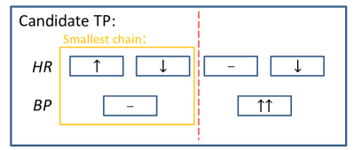
Figure 3: An example of an TP and its smallest starting chain.

When we check if $P$ is inside an MSS, we need to traverse only the states of $P_{chain}$ and the first state of $P_{end}$ if any is present because $P_{chain}$ may be pattern $P$ itself. It is easy to see since after we have arrived at $P_{chain}$ (we know it is there at this starting position) by recursive search function (Algorithm 4) and checked that all time relationship between the states of $P_{chain}$ are satisfied, we need to verify only that all the states of $P_{chain}$ are before the first state of $P_{end}$ since all the states of $P_{chain}$ will be before all the other states of $P_{end}$ by transitivity. Thus, we need to check $|P_{chain}|+1$ first states of $P$, if $P\neq P_{chain}$, and $|P_{chain}|$ first states of $P$, otherwise. We call this number exposure of $P$ and denote it as $exposure(P)$.

Input: P, D, id, i, positions, exposure

Output: Integer

while $i\leq|P.EVL[id].pos|$ do

       if Check accumulated time relationships in D[id] then

             if $exposure=0$ then return $\leavevmode\nobreak\ i$;

             $pos\leftarrow P.EVL[id].pos[i]$

             $ind\leftarrow P.EVL[id].ind[i]$

            

            return $Search(parent(P),D,id,ind,positions\cap\{pos\},exposure-1)$

            

       end if

      $i\leftarrow i+1$

      

end while

return $\leavevmode\nobreak\ -1$

Algorithm 4 Function $Search(P,D,id,ind,positions,exposure)$.

4 Computational Results

To evaluate the performance of the Fast Temporal Pattern Mining with Extended Vertical Lists (FTPMwEVL) algorithm, we tested it against the approach by Batal et al., from now on referred to as FTPM, on real-life datasets. The temporal pattern was defined as in Definition 2 for both algorithms.

All computations were carried out on a virtual server machine with 100 GB of memory and 20 virtual cores with processor speed equivalent to 2.5 GHz each. Only one core was utilized for single-thread computations. C++11 was used as a programming language. All computation times show actual pattern mining time taken by the algorithms after any preprocessing steps such as loading data and converting it into the abstraction domain.

It is important to state that the returned temporal patterns were entirely identical for both algorithms. It leaves computational time and memory usage as the only criteria for algorithm comparison.

4.1 Acute Kidney Injury dataset

The AKI dataset consists of $n=5202$ medical records composed of time series taken during surgical procedures [20, 21]. Each record has an outcome associated with it: 1, if Acute Kidney Injury (AKI) was diagnosed after the surgery (2769 records), and 0, otherwise (2433 records).

Using the University of Florida Integrated Data Repository, we have previously assembled a single center cohort of perioperative patients by integrating multiple existing clinical and administrative databases at UF Health [20, 21]. We included all patients admitted to the hospital for longer than 24 hours following any operative procedure between January 1, 2000, and November 30, 2010. This dataset was integrated with the laboratory, the pharmacy and the blood bank databases and intraoperative database (Centricity Perioperative Management and Anesthesia, General Electric Healthcare, Inc.) to create a comprehensive intraoperative database for this cohort. The study was designed and approved by the Institutional Review Board of the University of Florida and the University of Florida Privacy Office.

Two time variables were chosen for examination: Mean Arterial Blood Pressure (BP) and Heart Rate (HR). The value abstractions were used to convert time series from time domain to abstraction domain with percentile values $[0.1,0.25,0.75,0.9]$ and support threshold $\theta$ (see Definition • ‣ 4) ranging from $0.5$ to $0.9$. The comparative data (see Table 1) indicates the superior performance of FTPMwEVL from the computational time point of view. For $\theta=0.7$, FTPMwEVL found all FTPs (there were no FTPs of size more than 18) in $39.58$ seconds using $3134.2$ megabytes of memory, while FTPM spent $34280.4$ seconds and $402.31$ megabytes to achieve the same result. Therefore, the speed-up was of magnitude $\mathbf{866}$ while the new algorithm used only 7.79 times more memory. We set a computational time limit to 24 hours (86,400 seconds). In this time frame, FTPM was able to mine all FTPs only for $\theta\geq 0.7$. For $\theta=0.6$, FTPMwEVL found all FTPs (no FTPS of size more than 22), yet FTPM managed to mine FTPs of size 10 or lower and some of size 11. In this case, FTPMwEVL took $50.25$ seconds (not shown in the table) to mine all FTPs of size 11 or lower, and the speed-up column reflects ratio $86400\leavevmode\nobreak\ \text{sec}/50.25\leavevmode\nobreak\ \text{sec}=1719.3$. For $\theta=0.5$, we limited the maximum FTP size to 12 due to FTPMwEVL memory consumption considerations. Still, FTPM mined only FTPs of size 7 or lower and some of size 8 in 86400 seconds.

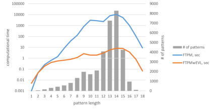
Figure 4: Computational time in seconds for FTPMwEVL and FTPM on AKI dataset for mining FTPs of sizes from 1 to 18 (there were no FTPs of a size larger than 19), given that all FTPs of smaller sizes were already found. Threshold $\theta$ was set at $0.7$. Total computational time was $34280.4$ and $39.58$ seconds for FTPM and FTPMwEVL, respectfully. Memory usage was $402.31$ and $3134.2$ megabytes. Thus, FTPMwEVL achieved a significant speed-up of magnitude $\mathbf{866}$ while consuming $7.79$ times more memory.

As can be seen from Figure 4, the Extended Vertical Lists start working significantly better than the regular vertical lists with increasing FTP size, which happens due to the better indexing strategy that allows eliminating more candidate TPs and validating that a TP is not an FTP faster. Table 1 demonstrates a phenomenon of exponential growth of computational time and memory usage with decreasing threshold level which is the main limitation of this pattern mining paradigm.

Table 1: Computational time comparison of FTPMwEVL and FTPM on AKI datasets.

$\theta$	max $k$	FTPM			FTPMwEVL			speed-up	mem. ratio
		k	sec	MB	k	sec	MB
0.9	Inf	7	0.16	1.86	7	0.1	15.8	1.06	8.49
0.8	Inf	12	465.5	24.92	12	2.3	198.5	$\mathbf{204.27}$	7.96
0.7	Inf	18	34280.4	402.31	18	39.6	3134.2	$\mathbf{866}$	7.79
0.6	Inf	10	$\mathbf{>86400}$	NA	22	621.1	35566.1	$\mathbf{>1719.3}$	NA
0.5	12	7	$\mathbf{>86400}$	NA	12	467.8	28950.4	$\mathbf{>998.93}$	NA

4.2 UCR Time Series Classification Archive

The remaining datasets were taken from UCR Time Series Classification Archive [22]. Out of 85 datasets available, only those that have two classes were picked what resulted in 31 datasets. In this archive, each record has only one time series which was converted into two series of time-interval states using both trend and value abstractions. Percentiles $[0.1,0.25,0.75,0.9]$ for value abstractions were used to mine patterns in the UCR datasets, where, e.g., all values falling between percentiles 0.1 and 0.25 were considered as low. For trend abstractions, a segment was considered increasing if the slope was positive, and non-increasing, otherwise. The support threshold $\theta$ and maximum size $k$ varied in ranges $[0.2,0.8]$ and $[5,\infty]$, respectfully, depending on the dataset complexity: we pushed the memory consumption of FTPMwEVL to the limit. Therefore, Table 2 reflects the most difficult cases from FTPMwEVL memory usage point of view.

FTPMwEVL was slower only on three datasets. The most significant speed-up of magnitude 3685.85 was achieved on dataset “Computers”. For this case, FTPMwEVL found all FTPs up to the predefined maximum size $k=14$ (it was set on this level due to memory considerations) in 446.08 seconds having used 26100.1 megabytes of memory. FTPM mined all FTPs of size 8 or lower and some of size 9 in the time frame of 86400 seconds. Similar to the AKI dataset, the speed-up column reflects ratio $86400\leavevmode\nobreak\ \text{sec}/\leavevmode\nobreak\ 23.44\leavevmode\nobreak\ \text{sec}=3685.85$, where 23.44 seconds is the running time of FTPMwEVL to find all FTPs of size 9 or lower. Speed-up of 30 times or more was achieved on four other datasets: the values in bold font. However, after removing these outliers, the speed-up was on the level of $2.34$ on average for the remaining datasets. The memory consumption was 4.15 time higher for FTPMwEVL on average. In the worst case, $35566.5$ megabytes of memory was allocated to store all FTPs which is not a concern for modern computational clusters.

Table 2: Computational time comparison of FTPMwEVL and FTPM on UCR datasets.

dataset	$\theta$	max $k$	FTPM			FTPMwEVL			speed-up	mem. ratio
			k	sec	MB	k	sec	MB
BeetleFly	0.8	8	8	702.0	5577.2	8	275.5	18367.7	2.55	3.29
BirdChicken	0.7	Inf	18	742.9	1564.4	18	269.9	4873.5	2.75	3.12
Coffee	0.8	10	10	560.1	4108.8	10	283.5	13107.4	1.98	3.19
Computers	0.8	14	8	$\mathbf{>86400}$	NA	14	446.1	26100.1	$\mathbf{>3685.8}$	NA
DistalPhalanx OutlineCorrect	0.7	Inf	16	160.3	1435.1	16	113.3	5382.6	1.41	3.75
Earthquakes	0.8	7	7	905.4	923.7	7	220.1	14340.2	4.11	15.52
ECG200	0.6	Inf	18	2349.7	3225.3	18	300.5	11863.1	7.82	3.68
ECGFiveDays	0.5	Inf	19	336.3	1181.4	19	226.1	3509.4	1.49	2.97
FordA	0.8	5	5	214.9	1462.2	5	113.4	11068.7	1.90	7.57
FordB	0.8	5	5	125.9	891.0	5	59.9	6461.7	2.10	7.25
Gun_Point	0.2	Inf	18	35.3	129.6	18	27.0	377.7	1.31	2.91
Ham	0.8	7	7	783.8	5894.6	7	310.5	26318.9	2.52	4.46
HandOutlines	0.8	12	12	87.3	2847.4	12	134.9	9917.5	0.65	3.48
Herring	0.8	10	10	470.7	3186.7	10	177.9	10216.7	2.65	3.21
ItalyPowerDemand	0.2	Inf	13	1.2	16.8	13	1.4	46.4	0.86	2.75
Lighting2	0.8	8	8	50929.9	6080.6	8	495.1	35555.4	$\mathbf{102.87}$	5.85
MiddlePhalanx OutlineCorrect	0.7	Inf	17	301.6	2689.2	17	184.3	9633.6	1.64	3.58
MoteStrain	0.2	Inf	20	402.5	1109.5	20	380.6	2316.5	1.06	2.09
PhalangesOutlines Correct	0.5	Inf	14	96.6	1115.3	14	71.9	4035.1	1.34	3.62
ProximalPhalanx OutlineCorrect	0.4	Inf	19	588.0	4271.8	19	307.5	15383.3	1.91	3.60
ShapeletSim	0.8	7	6	$\mathbf{>86400}$	NA	7	378.1	25489.8	$\mathbf{>228.52}$	NA
SonyAIBORobot Surface	0.8	10	10	1387.0	5255.8	10	474.6	14650.9	2.92	2.79
SonyAIBORobot SurfaceII	0.8	10	10	2222.3	6619.7	10	701.0	21730.3	3.17	3.28
Strawberry	0.7	Inf	18	200.4	1701.7	18	105.9	6042.2	1.89	3.55
ToeSegmenta-tion1	0.8	8	8	754.7	2904.8	8	181.5	11128.0	4.16	3.83
ToeSegmenta-tion2	0.8	8	8	845.9	3076.6	8	188.2	10987.0	4.49	3.57
TwoLeadECG	0.2	Inf	17	15.1	93.5	17	15.2	243.1	0.99	2.60
wafer	0.7	Inf	11	$\mathbf{>86400}$	NA	29	275.6	10952.4	$\mathbf{>660.73}$	NA
Wine	0.7	Inf	22	481.8	4288.6	22	354.8	14043.6	1.36	3.27
WormsTwoClass	0.8	7	7	5459.6	2183.7	7	148.7	11036.3	$\mathbf{36.75}$	5.05
yoga	0.4	Inf	16	410.3	3593.7	16	215.6	8825.3	1.90	2.46

5 Concluding Remarks

In this paper, a new algorithm for Mining Frequent Temporal Patterns was presented where the concept of Extended Vertical List was utilized. It outperformed the existing approach on many real-life datasets in terms of computational time with minor exceptions. EVL requires more memory to be stored, which is a typical trade-off in such type of algorithms. The proof of concept is that server clusters and personal computers have enough memory nowadays. Moreover, memory is becoming cheaper significantly faster than CPU, as well as the memory size becomes five times of its previous size every two years (see http://www.jcmit.com/) while CPU resources only double during the same time frame [23]. Thus, the problem of using large amounts of memory is becoming less and less critical.

The speed-up was achieved due to EVL which works in two main directions: elimination of more candidate TPs, and faster verification of whether a candidate TP is an FTP or not. The candidate elimination by EVL works under the assumption that if a pattern is an FTP than all its subpatterns are FTPs as well. For other concepts of TP like Recent Temporal Pattern (RTP) in [10], this assumption does not hold. Thus, the candidate elimination phase will not work here, and only less efficient techniques like the Vertical Data Format should be utilized instead. Still, the concept of positions and indices will work for RTPs since the parent of an RTP is an RTP itself. Therefore, Extended Vertical Lists can give a partial speed-up for Frequent RTP Mining too. The approach can be generalized and applied to other domains where the notion of pattern is defined in other ways.

References

- [1] Jiawei Han, Jian Pei, Behzad Mortazavi-Asl, Helen Pinto, Qiming Chen, Umeshwar Dayal, and MC Hsu. Prefixspan: Mining sequential patterns efficiently by prefix-projected pattern growth. In proceedings of the 17th international conference on data engineering, pages 215–224, 2001.
- [2] Jay Ayres, Jason Flannick, Johannes Gehrke, and Tomi Yiu. Sequential pattern mining using a bitmap representation. In Proceedings of the eighth ACM SIGKDD international conference on Knowledge discovery and data mining, pages 429–435. ACM, 2002.
- [3] Jianyong Wang and Jiawei Han. Bide: Efficient mining of frequent closed sequences. In Data Engineering, 2004. Proceedings. 20th International Conference on, pages 79–90. IEEE, 2004.
- [4] Ding-Ying Chiu, Yi-Hung Wu, and Arbee LP Chen. An efficient algorithm for mining frequent sequences by a new strategy without support counting. In Data Engineering, 2004. Proceedings. 20th International Conference on, pages 375–386. IEEE, 2004.
- [5] Divya Iyer, Arti Mohanpurkar, Sneha Janardhan, Dhanashree Rathod, and Amruta Sardeshmukh. Credit card fraud detection using hidden markov model. In Information and Communication Technologies (WICT), 2011 World Congress on, pages 1062–1066. IEEE, 2011.
- [6] R. Agrawal and R. Srikant. Mining sequential patterns. In Data Engineering, 1995. Proceedings of the Eleventh International Conference on, pages 3–14, 1995.
- [7] Ramakrishnan Srikant and Rakesh Agrawal. Mining sequential patterns: Generalizations and performance improvements. Advances in Database Technology—EDBT’96, pages 1–17, 1996.
- [8] Lucia Sacchi, Cristiana Larizza, Carlo Combi, and Riccardo Bellazzi. Data mining with temporal abstractions: learning rules from time series. Data Mining and Knowledge Discovery, 15(2):217–247, 2007.
- [9] Milos Hauskrecht, Shyam Visweswaran, Gregory F Cooper, and Gilles Clermont. Data-driven identification of unusual clinical actions in the icu. In AMIA, 2013.
- [10] Iyad Batal, Gregory F Cooper, Dmitriy Fradkin, James Harrison Jr, Fabian Moerchen, and Milos Hauskrecht. An efficient pattern mining approach for event detection in multivariate temporal data. Knowledge and information systems, 46(1):115–150, 2016.
- [11] Robert Moskovitch and Yuval Shahar. Classification-driven temporal discretization of multivariate time series. Data Mining and Knowledge Discovery, 29(4):871–913, 2015.
- [12] Rakesh Agrawal, Ramakrishnan Srikant, et al. Fast algorithms for mining association rules. In Proc. 20th int. conf. very large data bases, VLDB, volume 1215, pages 487–499, 1994.
- [13] Mohammed Javeed Zaki. Scalable algorithms for association mining. IEEE Transactions on Knowledge and Data Engineering, 12(3):372–390, 2000.
- [14] Mohammed J Zaki. Spade: An efficient algorithm for mining frequent sequences. Machine learning, 42(1):31–60, 2001.
- [15] Eamonn Keogh, Selina Chu, David Hart, and Michael Pazzani. Segmenting time series: A survey and novel approach. Data mining in time series databases, 57:1–22, 2004.
- [16] James F Allen. Towards a general theory of action and time. Artificial intelligence, 23(2):123–154, 1984.
- [17] Iyad Batal, Lucia Sacchi, Riccardo Bellazzi, and Milos Hauskrecht. Multivariate time series classification with temporal abstractions. 2009.
- [18] Iyad Batal, Hamed Valizadegan, Gregory F Cooper, and Milos Hauskrecht. A pattern mining approach for classifying multivariate temporal data. In Bioinformatics and Biomedicine (BIBM), 2011 IEEE International Conference on, pages 358–365, 2011.
- [19] Iyad Batal, Dmitriy Fradkin, James Harrison, Fabian Moerchen, and Milos Hauskrecht. Mining recent temporal patterns for event detection in multivariate time series data. In Proceedings of the 18th ACM SIGKDD international conference on Knowledge discovery and data mining, pages 280–288, 2012.
- [20] Dmytro Korenkevych, Tezcan Ozrazgat-Baslanti, Paul Thottakkara, Charles E Hobson, Panos Pardalos, Petar Momcilovic, and Azra Bihorac. The pattern of longitudinal change in serum creatinine and 90-day mortality after major surgery. Annals of surgery, 263(6):1219–1227, 2016.
- [21] Paul Thottakkara, Tezcan Ozrazgat-Baslanti, Bradley B Hupf, Parisa Rashidi, Panos Pardalos, Petar Momcilovic, and Azra Bihorac. Application of machine learning techniques to high-dimensional clinical data to forecast postoperative complications. PloS one, 11(5):e0155705, 2016.
- [22] Yanping Chen, Eamonn Keogh, Bing Hu, Nurjahan Begum, Anthony Bagnall, Abdullah Mueen, and Gustavo Batista. The ucr time series classification archive. www.cs.ucr.edu/~eamonn/time_series_data/, July 2015.
- [23] Gordon E Moore et al. Progress in digital integrated electronics. In Electron Devices Meeting, volume 21, pages 11–13, 1975.