A Functional Mapping for Passively Mode-Locked Semiconductor Lasers

Abstract

We present a novel approach for the analysis of passively mode-locked semiconductor lasers that allows for efficient parameter sweeps and time jitter analysis. It permits accessing the ultra-low repetition rate regime where pulses become localized states. The analysis including slow (e.g. thermal) processes or transverse dynamics becomes feasible. Our method bridges the divide between the phenomenological, yet highly efficient, pulse iterative model that is the Haus master equation, and the more involved first principle descriptions relying on time delayed equations. Our iterative functional mapping exploits the fundamental division of the mode-locking regime between fast and slow stages and allows computing the dynamics only in the pulse vicinity. Reductions of the simulation times and of the memory footprint up to two orders of magnitudes are demonstrated. Finally, the mapping also provides a general framework for deducing the Haus master equation from first principle models based upon delayed differential equations.

Generation of low repetition rate picosecond pulses is of paramount importance for a number of applications KT-PR-06 ; lidar . Passive Mode-locking (PML) of semiconductor lasers is a most promising method, although it still represents an experimental and a theoretical challenge, see AJ-BOOK-17 for a recent review. The Haus master equation haus00rev is an efficient and widely used approach to study PML. It consists in restricting the analysis of the field to a small temporal interval around the pulse. Yet this method, when applied to a particular design, provides only qualitative predictions due to the many simplifying hypothesis involved. How to derive the Haus equation, for a specific laser design, is also an open question. On the other hand, first principle modeling allows representing the full dynamics of both unidirectional and bidirectional cavities as either Delay Differential Equations (DDEs) VT-PRA-05 or Delay Algebraic Equations (DAEs) MB-JQE-05 , respectively. Such models have been applied successfully to the study of PML with saturable absorber (SA), and extended to describe photonic crystals HBM-OE-10 , external optical feedback JNS-PRE-16 , optical injection RHR-PRE-11 ; AHP-JOSAB-16 , frequency swept sources SKO-OE-13 , quantum dot lasers RBM-JQE-11 , nonlocal imaging conditions MJB-JSTQE-15 and localized structures (LSs) MJB-PRL-14 .

The understanding of PML is limited by its strongly multiscale nature, in which the field and the gain temporal features differ by several orders of magnitudes. Even semiconductor mode-locked lasers, that have fast gain recovery $\tau_{g}\sim 1\,$ns, generate pulses of a duration $\tau_{p}\sim 1\,$ps, hence $\tau_{p}/\tau_{g}\ll 1$. Finding the optimal operating regimes and studying the pulse train’s amplitude and temporal jitter require simulations over hundreds of thousands of round-trips. If, in addition to the longitudinal dynamics, transverse diffraction of the beam or slow (e.g. thermal) processes are taken into account, the problem becomes quickly intractable. External cavity devices are of particular interest for low frequency PML. These configurations rely on vertical external-cavity surface-emitting semiconductor lasers (VECSELs) coupled to distant saturable absorber mirrors SESAMs hoogland00 ; haring01 ; haring02 ; tropper04 . Recently, a regime of temporal localization allowing arbitrary low repetition rates was demonstrated in such systems MJB-PRL-14 ; CJM-PRA-16 ; JCM-PRL-16 . In this regime in which the cavity round-trip $\tau$ is much larger than $\tau_{g}$, the PML pulses become individually addressable temporal LSs, that could also evolve into three-dimensional light bullets J-PRL-16 ; GJ-PRA-17 if broad-area VECSELs are considered. However, the analysis in the regime $\tau\gg\tau_{g}\gg\tau_{p}$ is particularly tedious. All these arguments call for the development of more efficient methods.

In this manuscript, we present an approach that combines the accuracy of first principle time-delayed models with the computational efficiency of the Haus master equation. Our method is based upon computing only the so-called fast stage in the vicinity of the pulse where stimulated emission is dominant, while using the analytical solution of the dynamics during the slow stage in-between pulses. In the latter, pumping and carrier recombination are the dominant processes, and the dynamics essentially consists in the exponential recovery of the gain and of the absorption. Further, one reconnects this analytically found slow-stage solution to the next round-trip’s fast stage as a connecting boundary condition. This idea is general and it is applicable to any model described by DDEs or DAEs, and generally to all PML lasers in which fast and slow stages can be identified.

We illustrate the idea of the functional mapping (FM) using the DDE model of VT-PRA-05 that considers unidirectional propagation in a ring laser. The equations for the field amplitude $A$, the gain $G$ and the absorption $Q$ read

$$\frac{\dot{A}}{\gamma} = -A+Y\left(t-\tau\right),$$ (1)

$$\dot{G} = \Gamma\left(G_{0}-G\right)-e^{-Q}\left(e^{G}-1\right)\left|A\right|^{2},$$ (2)

$$\dot{Q} = Q_{0}-Q-s\left(1-e^{-Q}\right)\left|A\right|^{2},$$ (3)

with

$$Y\left(t\right) = \sqrt{\kappa}\exp\left[\frac{1-i\alpha}{2}G\left(t\right)-\frac{1-i\beta}{2}Q\left(t\right)\right]A\left(t\right),$$ (4)

and $G_{0}$ the pumping strength, $\Gamma=\tau_{g}^{-1}$ the gain recovery rate, $Q_{0}$ the value of the unsaturated losses which determines the modulation depth of the SA and $s$ the ratio of the saturation energy of the gain and of the SA sections. We define $\kappa$ as the intensity transmission of the output mirror, i.e., the fraction of the power remaining in the cavity after each round-trip. In Eqs. (1-3) time has been normalized to the SA recovery time that we assume to be $\tau_{q}=20\,$ps. The linewidth enhancement factor of the gain and absorber sections are noted $\alpha$ and $\beta$, respectively. In addition, $\gamma$ is the bandwidth of the spectral filter whose central optical frequency has been taken as the carrier frequency for the field. This spectral filter may (coarsely) represent, e.g., the resonance of a VCSEL MJB-JSTQE-15 . If not otherwise stated $\left(\kappa,\alpha,\beta,s\right)=\left(0.8,2,0.5,30\right)$, and $Q_{0}=0.3$ which corresponds to modulation of the losses of $\sim 26\,\%$. We also set $\gamma=10$ and $\Gamma=0.04$, leading to a gain bandwidth full width at half maximum of $160\,$GHz and $\tau_{g}=500\,$ps.

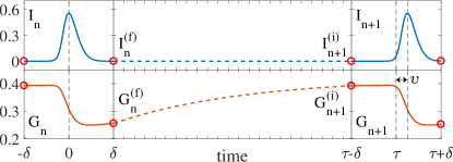
Figure 1: Temporal profile of the intensity $I_{n}=\left|A_{n}\right|^{2}$ and of the gain $G_{n}$ at the $n$-th and $n+1$-th round-trips. After the emission of the pulse $I_{n}$ and the ensuing gain depletion, the so-called fast stage (solid lines), the gain recovers until the next round-trip while the field is vanishing (dashed lines). Knowing the final value of $G_{n}^{\left(f\right)}$ in the interval $z\in\left[-\delta,\delta\right]$, one can deduce the initial gain value at the next round-trip $G_{n+1}^{\left(i\right)}$. The central panel (not up to scale) can be several orders of magnitude larger than the outer panels.

We wrote Eq. (1) in a form that makes apparent that the forcing field $Y\left(t-\tau\right)$ defined in Eq. (4) is a nonlinear function that is known over a whole interval of duration $\tau$. Since $G$ and $Q$ are functions of $A$, $Y$ involves only the past values of the field, i.e., $Y\left(t-\tau\right)=g\left[A\left(t-\tau\right)\right]$. Knowing the forcing term $Y$, Eq. (1) can be solved for $A$ over an interval of duration $\tau$. Integrating Eqs. (1-4), not over the whole round-trips, but only in a selected time interval in the pulse vicinity, is at the core of our method. We define the field and carrier profiles at the $n$-th round-trip as $A_{n}\left(z\right)$ and $\left(G_{n},Q_{n}\right)\left(z\right)$. For clarity, we set in Fig. 1 the pulse at the origin of time at the $n$-th round-trip. Next, we define a small interval of duration $2\delta$ and a local time $z\in\left[-\delta,\delta\right]$. Finally, we impose a condition on the waveform $A_{n}$: it is a pulse of duration $\tau_{p}$ asymptotic to $A=0$ if $\delta\gg\tau_{p}$. Under these approximations, one can solve Eq. (1) using standard integration techniques, e.g., Runge-Kutta method, at the next round-trip, using the following sequence $\left(A_{n},G_{n},Q_{n}\right)\rightarrow Y_{n}\rightarrow\left(A_{n+1},G_{n+1},Q_{n+1}\right)$. Doing so corresponds to writing a functional mapping $A_{n+1}=F\left(A_{n}\right)$. The remainder of the dynamics during the round-trip of duration $r=t-2\delta$, see central panel in Fig. 1, in which the field is vanishing can be found by solving Eqs. (2,3) analytically in the absence of stimulated emission, the so-called slow stage of PML. As such, $G_{n+1}^{(i)}=G_{n}^{(f)}\chi+G_{0}\left(1-\chi\right)$ with $\chi=\exp\left(-\Gamma r\right)$ and similarly for $Q_{n+1}^{(i)}$. Solving analytically the slow stage allows to fully cancel the stiffness inherent to the multiscale nature of PML which is exceptionally useful in the long delay limit $\tau\gg\tau_{g}$. The speedup of our method is equal to the ratio of the actual integration domain $2\delta$ and of the full round-trip $\tau$, i.e., $m=\tau/\left(2\delta\right)$. Taking a domain of duration $2\delta=5\tau_{p}$, a pulse-with of $\tau_{p}=1\,$ps at a repetition rate of $\tau^{-1}=1\>$GHz, yields a speedup $m=200$, i.e., a 24 hour simulation with, e.g., slow thermal effects or transverse diffraction could potentially be achieved in a few ($\sim 7$) minutes. We stress that our method can potentially be extended to the case of a non zero background field. Such a situation could occur, e.g., in presence of monochromatic optical injection and in this case the PML pulses would exist on a non zero background field as in the Lugatio-Lefever model LL-PRL-87 . However, this background homogeneous state upon which the pulses connect asymptotically would need to be unconditionally stable.

Time-delayed systems are essentially convective GP-PRL-96 . As such, the period of the solution is always slightly different from the value of the time delay and the pulse $A_{n+1}$ at the next round-trip will be shifted, see Fig. 1 right panels. In the case of PML, this drift admits an intuitive interpretation: If the pulse at the $n$-th round-trip $A_{n}$ is centered, the next iterate of the pulse $A_{n+1}$ will slightly by shifted to the right, of an amount $\upsilon=\gamma^{-1}$, as a consequence of the inertia of the resonant filter. An effect modeled by the parameter $\gamma$ that represents for the case of a VCSEL, the time the photons remain trapped in the cavity. The pulse can also deviate from the center of the interval due to stochastic fluctuations. Hence, one needs to recenter the pulse at each round-trip leading directly to the value of the pulse jitter.

Our method is, in addition, a rigorously way to deduce the Haus master equation in a general setting. For the case of Eqs. (1-4), one can use the Fourier transform $\mathcal{F}$ yielding an explicit, expression of the mapping operator

$$A_{n+1} = \mathcal{F}^{-1}\left[\mathcal{L}\left(\omega\right)\mathcal{F}\left[g\left(A_{n}\right)\right]\right],$$ (5)

where we defined the Lorentzian kernel $\mathcal{L}\left(\omega\right)=\left(1+i\omega/\gamma\right)^{-1}$ . The fact that equations of the type as Eq. (1) could be solved by a Fourier method was already pointed out in GP-PRL-96 for the case of a single variable. The nominal drift can easily be accounted for setting $\mathcal{L}\left(\omega\right)\rightarrow\mathcal{L}\left(\omega\right)\exp\left(i\omega\upsilon\right)$ with $\upsilon=\gamma^{-1}$. Introducing a slow time scale for the evolution of the field after each round-trip as $\partial A/\partial\xi=A_{n+1}-A_{n}$, we find

$$\frac{\partial A}{\partial\xi} \equiv \mathcal{F}^{-1}\left[\mathcal{L}\left(\omega\right)\mathcal{F}\left[g\left(A_{n}\right)\right]\right]-A_{n}.$$ (6)

By inspecting Eq. (6), one can notice how obtaining the Haus equation necessitates a wealth of approximations. One needs to assume the uniform field limit (UFL), i.e. small gain, absorption, and losses, and phase change. In addition, we expand in Taylor series $\mathcal{L}\left(\omega\right)$ and truncate to second order in $\omega$. Finally, we find setting $i\omega\rightarrow\partial/\partial z$

$$\frac{\partial A}{\partial\xi} = \left\{\sqrt{\kappa}\left(1+\frac{1-i\alpha}{2}G-\frac{1-i\beta}{2}Q\right)-1+\frac{1}{2\gamma^{2}}\frac{\partial^{2}}{\partial z^{2}}\right\}A.$$ (7)

It was under these approximations that the Haus equation was derived from Eqs. (1-3) using the multiple time scales formalism in KNE-PD-06 ; CJM-PRA-16 . We also note that even in the UFL, the Haus equation remains an approximation. A continuous dynamical system can not emulate correctly a discrete mapping. In addition, writing a parabolic partial differential equation remains an approximation of the time delayed operator $\mathcal{L}\left(\omega\right)$ described by a Lorentzian, only valid for narrow bandwidth fields.

The FM can be used to study the dynamics of the pulse, like the leading and trailing edge instabilities, and in general the unstable regimes where the pulse breathes in height and width. At variance with the Haus equation, we will show in Fig. 3 that the gain induced instabilities, such as self-pulsation, are also conserved due to the proper consideration of the gain recovery dynamics. However, we note that the FM suffers from the same limitation than all pulse iterative models, i.e., the modal structure of the laser is lost and so are the transitions toward harmonic PML, so that in the FM, it is essential to assume the background stability criterion. However, we note that this potential weakness can be mitigated since the Harmonic transition is relatively easy to predict by monitoring the maximal value of the net gain during its recovery. As long as it remains negative, the spontaneous transitions toward Harmonic PML is inhibited.

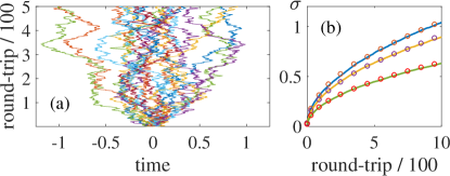
Figure 2: Temporal jitter of the pulse in the fundamental PML regime. (a) Twenty different realizations leading to uncorrelated random walks. (b) Variance of the random walk for different parameters that correspond from top to bottom to the short i), medium ii) and long iii) cavity regimes, see text for details. The lines and the circles correspond to the DDE model (1-4) and the FM (5), respectively.

While the stiffness of PML could, in principle, be alleviated by the use of adaptive time-step method, these algorithms do not allow for stochastic analysis and to include transverse effects such as diffraction, which can easily be studied with the FM. We show in Fig. 2 the results of a time jitter analysis, either integrating Eqs. (1-4) or the FM given by Eq. (5). For the sake of simplicity, we added white delta correlated noise of variance $\sigma_{e}=10^{-2}$ in the field equation only, but similar fluctuations could be introduced in the carrier equations to model current fluctuations. We performed statistics in different regimes, the short i) $\left(G_{0},\tau\right)=\left(0.6,5\right)$, average ii) $\left(G_{0},\tau\right)=\left(0.5,10\right)$, and long iii) $\left(G_{0},\tau\right)=\left(0.4,100\right)$ cavities. The domain length hosting the pulse in the FM is $2\delta=3.$ Statistics were performed averaging the pulse jitter over $N_{r}=10^{4}\,$realizations of $10^{3}\,$round-trips. A few trajectories are depicted in Fig. 2 (a) to exemplifies the random walk that the pulse performs from one round-trip toward the next while Fig. 2 (b) depicts the statistical variance $\sigma$ of the pulse distribution, that grows as $\sigma=\sqrt{2Dt}$ as predicted by the theory of Brownian motion. We notice that the FM yields identical results for the diffusion coefficient than the DDE model (1-4). However, such jitter results can be obtained in a few minutes using the FM, and the time necessary does not increase with the value of $\tau$. The agreement between the two approaches stem from the fact that the neutral mode that corresponds to the translation of the pulse in time is correctly preserved by the FM. We note that the value of $\sigma_{e}$ used leads to very large jitter, demonstrating that both methods are in agreement, even for large pulse to pulse deviations ($\sim 10\,\%$ in peak intensity). Large $\sigma_{e}$ allows to mitigate the finite size fluctuations proportional to $1/\sqrt{N_{r}}$ upon averaging over realizations. Performing a similar comparison for lower values of $\sigma_{e}$ would require prohibitively longer integration of Eqs. (1-4). Here, the semi-analytical method of JPR-PRA-15 should be used instead to compare with the FM.

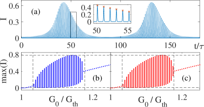
Figure 3: (a) Temporal trace of the self-pulsing regime found close to the lasing threshold $G_{th}$ , obtained for $\tau=2$ and $Q_{0}=0.6$ . The bifurcation diagrams recording the pulses intensity maxima are represented in (b) for the DDE model (1-4) and (c) for the FM (5). Residual differences can be found.

In the long cavity limit that allows for temporal pulses to become temporal LSs MJB-PRL-14 ; JCM-PRL-16 , all the bifurcation diagrams we performed as a function of all possible parameters led to a perfect superposition between the DDE model and the FM, the later leading to greatly reduced integration time. While in the short cavity regimes, i.e., $10\,$GHz and beyond, the use of the FM leads to less marked improvements, we demonstrate in Fig. 3 that even the self-pulsation region found in the vicinity of the threshold is preserved. The self-pulsation (SP) regime is found in high frequency semiconductor mode-locked lasers and it consists in relaxation oscillations between the pulse energy and the population inversion. A proper consideration of the carrier dynamics from one round-trip toward the next is essential to reproduce the dynamics of SP, that is not found in the Haus equation. We show in Fig. 3 (a) a temporal trace of the SP regime found close to the lasing threshold $G_{th}=Q_{0}-\log\kappa$, whereas the bifurcation diagrams showing the pulses intensity maxima are represented in panels (b) and (c) for the DDE (Eqs. 1-4) and the FM (Eq. 5), respectively. One can clearly see that the onset and disappearance of SP is well preserved by the FM, since the correlations between the gain and the field intensity from one round-trip to the next are properly accounted for. Here, $\tau=2$ and $Q_{0}=0.6$ which corresponds to a $25\,$GHz repetition rate and a $45\,\%$ modulation of the losses. The domain size in the FM is $2\delta=1.5.$ We note that for high frequency PML other modeling approaches such as Traveling Wave Models JB-JQE-10 ; JB-PRA-10 ; Freetwm are better indicated.

We conclude our analysis by showing how the FM can be used for the simulation of broad area MIXSEL system described by the DAE model of MB-JQE-05 ; MJB-JSTQE-15 . The model for the intra-cavity field $E$, gain $N_{1}$ and absorption $N_{2}$ reads

$$\dot{E} = \left[\left(1-i\alpha_{1}\right)N_{1}+\left(1-i\alpha_{2}\right)N_{2}-1+i\Delta_{\perp}\right]E+hY,$$ (8)

$$\dot{N}_{1} = \gamma_{1}\left(J_{1}-N_{1}\right)-N_{1}\left|E\right|^{2}\,,$$ (9)

$$\dot{N}_{2} = \gamma_{2}\left(J_{2}-N_{2}\right)-sN_{2}\left|E\right|^{2}\,.$$ (10)

while the relation linking the intra-cavity and the external cavity $Y$ fields is, after proper normalization that considers the cavity enhancement factor, $Y=\eta\left[E\left(t-\tau\right)-Y\left(t-\tau\right)\right]$ with $\eta$ the external mirror reflectivity. The coupling of $Y$ into the MIXSEL cavity is given by the parameter $h$, see MJB-JSTQE-15 for more details. We operate in the long cavity limit, such that $\chi=0$ and the value of $\tau$ is irrelevant. For the sake of simplicity, we only consider diffraction in a single transverse dimension, making the problem two-dimensional and allowing for easier multi-parameter bifurcation analysis. We concentrate on the spatio-temporal localization regime. Here, the PML pulses become temporal dissipative solitons that can be addressed individually, but at the same time, they also acquire a well defined transverse size. This regime where the field coalesces into a spatio-temporal soliton is called a Light Bullet (LB) J-PRL-16 ; GJ-PRA-17 .

Figure 4 (a) shows a two-dimensional bifurcation diagram for the case $\alpha_{j}=0$ as a function of the bias in the gain and absorber sections $J_{1}$ and $J_{2}$. Finding the region of stability in Fig. 4 (a) required 24 hours on a standard PC using the FM, instead of several months integrating the full DAE system. Figure 4 (b) depicts the spatio-temporal LB profile obtained with the FM method. Figure 4 (b) corresponds to a snapshot of the intracavity field with $t$ the temporal (cavity) axis and $x$ the transverse dimension.

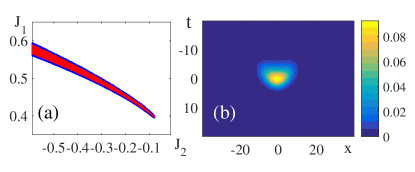
Figure 4: (a) Two-dimensional bifurcation diagram showing the region of stable existence of the LBs of the DAE model (8-10) as a function of the reverse bias in the gain and absorber sections $J_{1}$ and $J_{2}$. (b) Spatio-temporal profile of the field found with the FM with $\left(J_{1},J_{2}\right)=\left(0.498,-0.336\right)$. Other parameters are $\left(\alpha_{1},\alpha_{2},h,\gamma_{1},\gamma_{2},s,\eta\right)=\left(0,0,2,0.003,0.1,30,0.5\right)$.

In conclusion, we presented a modern approach for the analysis of PML in semiconductor lasers based upon a functional mapping and demonstrated its usefulness for parameter sweeps, time jitter analysis and spatio-temporal dynamics. In particular, the ultra-low repetition rate regime where the pulses become temporal LSs can be accessed easily, even in the presence of transverse effects. Our method also provides a general framework for deducing the Haus master equation from all models based upon delayed differential equations. While the Haus equation can be recovered in the uniform field limit, the FM possesses a stronger regime of applicability, in particular in the regime of strong gain and absorption, and we anticipate that significant deviations between DDE or DAE models and the Haus equations can be obtained, which will be the subject of further studies. Finally, we showed that the strong reduction in the degrees of freedom is also useful for studying transverse beam dynamics and more generally transverse patterns in PML. While the dynamics in presence of transverse and/or slow effects such as diffraction or thermal lensing is a topic of further studies, we gave an example how a multi-dimensional bifurcation diagram for Light Bullets can be obtained by means of the functional mapping method.

Funding information

MINECO Project COMBINA (TEC2015-65212-C3-3-P).

References

- (1) U. Keller and A. C. Tropper, “Passively modelocked surface-emitting semiconductor lasers,” Physics Reports 429, 67 – 120 (2006).
- (2) N. Takeuchi, N. Sugimoto, H. Baba, and K. Sakurai, “Random modulation cw lidar,” Appl. Opt. 22, 1382–1386 (1983).
- (3) E. Avrutin and J. Javaloyes, Mode-Locked Semiconductor Lasers, Book Chapter In: Handbook of Optoelectronic Device Modeling and Simulation (CRC press, Taylor and Francis, United Kingdom, 2017).
- (4) H. A. Haus, “Mode-locking of lasers,” IEEE J. Selected Topics Quantum Electron. 6, 1173–1185 (2000).
- (5) A. G. Vladimirov and D. Turaev, “Model for passive mode locking in semiconductor lasers,” Phys. Rev. A 72, 033808 (2005).
- (6) J. Mulet and S. Balle, “Mode locking dynamics in electrically-driven vertical-external-cavity surface-emitting lasers,” Quantum Electronics, IEEE Journal of 41, 1148–1156 (2005).
- (7) M. Heuck, S. Blaaberg, and J. Mørk, “Theory of passively mode-locked photonic crystal semiconductor lasers,” Opt. Express 18, 18003–18014 (2010).
- (8) L. Jaurigue, O. Nikiforov, E. Schöll, S. Breuer, and K. Lüdge, “Dynamics of a passively mode-locked semiconductor laser subject to dual-cavity optical feedback,” Phys. Rev. E 93, 022205 (2016).
- (9) R. M. Arkhipov, T. Habruseva, A. Pimenov, M. Radziunas, S. P. Hegarty, G. Huyet, and A. G. Vladimirov, “Semiconductor mode-locked lasers with coherent dual-mode optical injection: simulations, analysis, and experiment,” J. Opt. Soc. Am. B 33, 351–359 (2016).
- (10) N. Rebrova, G. Huyet, D. Rachinskii, and A. G. Vladimirov, “Optically injected mode-locked laser,” Phys. Rev. E 83, 066202 (2011).
- (11) S. Slepneva, B. Kelleher, B. O’Shaughnessy, S. Hegarty, A. Vladimirov, and G. Huyet, “Dynamics of fourier domain mode-locked lasers,” Opt. Express 21, 19240–19251 (2013).
- (12) M. Rossetti, P. Bardella, and I. Montrosset, “Modeling passive mode-locking in quantum dot lasers: A comparison between a finite-difference traveling-wave model and a delayed differential equation approach,” Quantum Electronics, IEEE Journal of 47, 569 –576 (2011).
- (13) M. Marconi, J. Javaloyes, S. Balle, and M. Giudici, “Passive mode-locking and tilted waves in broad-area vertical-cavity surface-emitting lasers,” Selected Topics in Quantum Electronics, IEEE Journal of 21, 85–93 (2015).
- (14) M. Marconi, J. Javaloyes, S. Balle, and M. Giudici, “How lasing localized structures evolve out of passive mode locking,” Phys. Rev. Lett. 112, 223901 (2014).
- (15) S. Hoogland, S. Dhanjal, A. C. Tropper, J. S. Roberts, R. Häring, R. Paschotta, F. Morier-Genoud, and U. Keller, “Passively mode-locked diode-pumped surface-emitting semiconductor lasers,” IEEE Photonics Technology Letters 12, 1135–1137 (2000).
- (16) R. Häring, R. Paschotta, E. Gini, F. Morier-Genoud, D. Martin, H. Melchior, and U. Keller, “Picosecond surface-emitting semiconductor laser with 200 mW average output power,” Electronics Letters 37, 766–768 (2001).
- (17) R. Häring, R. Paschotta, A. Aschwanden, E. Gini, F. Morier-Genoud, and U. Keller, “High-power passively mode-locked semiconductor lasers,” Quantum Electronics, IEEE Journal of 38, 1268–1275 (2002).
- (18) A. C. Tropper, H. D. Foreman, A. Garnache, K. G. Wilcox, and S. H. Hoogland, “Vertical-external-cavity semiconductor lasers,” J. Phys. D: Appl. Phys. 37, R75–R85 (2004).
- (19) P. Camelin, J. Javaloyes, M. Marconi, and M. Giudici, “Electrical addressing and temporal tweezing of localized pulses in passively-mode-locked semiconductor lasers,” Phys. Rev. A 94, 063854 (2016).
- (20) J. Javaloyes, P. Camelin, M. Marconi, and M. Giudici, “Dynamics of localized structures in systems with broken parity symmetry,” Phys. Rev. Lett. 116, 133901 (2016).
- (21) J. Javaloyes, “Cavity light bullets in passively mode-locked semiconductor lasers,” Phys. Rev. Lett. 116, 043901 (2016).
- (22) S. V. Gurevich and J. Javaloyes, “Spatial instabilities of light bullets in passively-mode-locked lasers,” Phys. Rev. A 96, 023821 (2017).
- (23) L. A. Lugiato and R. Lefever, “Spatial dissipative structures in passive optical systems,” Phys. Rev. Lett. 58, 2209–2211 (1987).
- (24) G. Giacomelli and A. Politi, “Relationship between delayed and spatially extended dynamical systems,” Phys. Rev. Lett. 76, 2686–2689 (1996).
- (25) T. Kolokolnikov, M. Nizette, T. Erneux, N. Joly, and S. Bielawski, “The q-switching instability in passively mode-locked lasers,” Physica D: Nonlinear Phenomena 219, 13 – 21 (2006).
- (26) L. Jaurigue, A. Pimenov, D. Rachinskii, E. Schöll, K. Lüdge, and A. G. Vladimirov, “Timing jitter of passively-mode-locked semiconductor lasers subject to optical feedback: A semi-analytic approach,” Phys. Rev. A 92, 053807 (2015).
- (27) J. Javaloyes and S. Balle, “Mode-locking in semiconductor Fabry-Pérot lasers,” Quantum Electronics, IEEE Journal of 46, 1023 –1030 (2010).
- (28) J. Javaloyes and S. Balle, “Quasiequilibrium time-domain susceptibility of semiconductor quantum wells,” Phys. Rev. A 81, 062505 (2010).
- (29) J. Javaloyes and S. Balle, “Freetwm: a simulation tool for multisection semiconductor lasers,” http://onl.uib.es/softwares (2012).