Rotational magnetocaloric effect of anisotropic giant spin systems

Abstract

The magnetocaloric effect, that consists of adiabatic temperature changes in a varying external magnetic field, appears not only when the amplitude is changed, but in cases of anisotropic magnetic materials also when the direction is varied. In this article we investigate the magnetocaloric effect theoretically for the archetypical single molecule magnets Fe₈ and Mn₁₂ that are rotated with respect to a magnetic field. We complement our calculations for equilibrium situations with investigations of the influence of non-equilibrium thermodynamic cycles.

1 Introduction

Magnetocalorics is an important thermodynamic concept with many applications for instance in room-temperature or sub-kelvin cooling [1, 2, 3, 4, 5, 6, 7]. It rests to a large extend on the magnetocaloric effect (MCE) [8] which states that in adiabatic processes, i.e. processes with constant entropy, the temperature changes upon the variation of the external magnetic field. Nowadays’s research efforts focus e.g. on new materials [9, 10, 11] or theoretical optimization of (molecular) magnetic materials [12, 13, 14, 15].

While the typical magnetocaloric process employs variations of the magnitude of the external field, some ideas focus on the effect of a rotation of the field or equivalently of the sample [16, 17, 18, 19]. A practical reason for this approach is given by the fact that mechanical rotations of the sample can be performed much more quickly than field sweeps. However, the rotational magnetocaloric effect (rMCE) requires anisotropic magnetic materials [20, 21]. In this article we therefore discuss how single-molecule magnets (SMM) perform as cooling agents in the kelvin temperature region. These materials are usually known for two other effects: slow relaxation and quantum tunneling of the magnetization [22, 23, 24, 25] and not considered for magnetic cooling in the ordinary sense. Nevertheless, their large anisotropy makes them prospective candidates for the rMCE [18].

In this article we investigate two aspects of the rMCE. We first discuss the isentropes and isothermal entropy changes that can be achieved in SMMs such as Fe₈ and Mn₁₂. In a second part we set up a simple relaxation dynamics in order to estimate how more realistic time-dependent Carnot processes would perform for these molecular coolers.

The article is organized as follows. In section 2 we introduce the model. Section 3 deals with the equilibrium rotational magnetocaloric effect whereas section 4 discusses dynamical aspects. Our results are summarized in section 5.

2 Model and numerical procedures

2.1 Model Hamiltonians

The low-temperature properties of single-molecule magnets with a large spectral gap between the ground state multiplet and higher-lying states can be rationalized using the giant spin approximation. To this end the zero-field split ground state multiplet is generated by an effective one-spin Hamiltonian. For Fe₈ the following giant spin Hamiltonian was developed [25]

$$\!\hbox{}\mathop{\vphantom{H}\smash{H}}\limits_{\sim}\!{}_{\text{Fe${}_{8}$}} = D_{\text{Fe${}_{8}$}}\;\!\hbox{}\mathop{\vphantom{S}\smash{S}}\limits_{\sim}\!{}_{z}^{2}+E_{\text{Fe${}_{8}$}}\;\left(\!\hbox{}\mathop{\vphantom{S}\smash{S}}\limits_{\sim}\!{}_{x}^{2}-\!\hbox{}\mathop{\vphantom{S}\smash{S}}\limits_{\sim}\!{}_{y}^{2}\right)+g_{\text{Fe${}_{8}$}}\,\mu_{B}\,\vec{B}(t)\cdot\!\hbox{}\mathop{\vphantom{\vec{S}}\smash{\vec{S}}}\limits_{\sim}\hbox{}\!$$

$$+B_{4,\text{Fe${}_{8}$}}^{0}\;\!\hbox{}\mathop{\vphantom{O}\smash{O}}\limits_{\sim}\!{}_{4}^{0}+B_{4,\text{Fe${}_{8}$}}^{2}\;\!\hbox{}\mathop{\vphantom{O}\smash{O}}\limits_{\sim}\!{}_{4}^{2}+B_{4,\text{Fe${}_{8}$}}^{4}\;\!\hbox{}\mathop{\vphantom{O}\smash{O}}\limits_{\sim}\!{}_{4}^{4}\ ,$$

with specific values of $S=10$, $D_{\text{Fe${}_{8}$}}=-0.295$ K, $E_{\text{Fe${}_{8}$}}=0.05605$ K, $|E_{\text{Fe${}_{8}$}}/D_{\text{Fe${}_{8}$}}|=0.19$, $B_{4,\text{Fe${}_{8}$}}^{0}=2.3\cdot 10^{-6}$ K, $B_{4,\text{Fe${}_{8}$}}^{2}=-7.2\cdot 10^{-6}$ K, $B_{4,\text{Fe${}_{8}$}}^{4}=-1.2\cdot 10^{-5}$ K, and $g_{\text{Fe${}_{8}$}}=2.0$ [26].

In the case of Mn₁₂, Hamiltonian (2.1) proved to be appropriate

$$\!\hbox{}\mathop{\vphantom{H}\smash{H}}\limits_{\sim}\!{}_{\text{Mn${}_{12}$}} = D_{\text{Mn${}_{12}$}}\;\!\hbox{}\mathop{\vphantom{S}\smash{S}}\limits_{\sim}\!{}_{z}^{2}+g_{\text{Mn${}_{12}$}}\,\mu_{B}\,\vec{B}(t)\cdot\!\hbox{}\mathop{\vphantom{\vec{S}}\smash{\vec{S}}}\limits_{\sim}\hbox{}\!$$

$$+B_{4,\text{Mn${}_{12}$}}^{0}\;\!\hbox{}\mathop{\vphantom{O}\smash{O}}\limits_{\sim}\!{}_{4}^{0}+B_{4,\text{Mn${}_{12}$}}^{4}\;\!\hbox{}\mathop{\vphantom{O}\smash{O}}\limits_{\sim}\!{}_{4}^{4}\ ,$$

with specific values of $S=10$, $D_{\text{Mn${}_{12}$}}=-0.65$ K, $B_{4,\text{Mn${}_{12}$}}^{0}=-3.0\cdot 10^{-5}$ K, $B_{4,\text{Mn${}_{12}$}}^{4}=\pm 4.6\cdot 10^{-5}$ K, and $g_{\text{Mn${}_{12}$}}=2.0$ [27]. Higher order spin operators are expressed by means of Stevens operators

$$\!\hbox{}\mathop{\vphantom{O}\smash{O}}\limits_{\sim}\!{}_{4}^{0} = 35\!\hbox{}\mathop{\vphantom{S}\smash{S}}\limits_{\sim}\!{}_{z}^{4}-\left[30S\left(S+1\right)-25\right]\!\hbox{}\mathop{\vphantom{S}\smash{S}}\limits_{\sim}\!{}_{z}^{2}+3S^{2}\left(S+1\right)^{2}-6S\left(S+1\right)$$ (3)

$$\!\hbox{}\mathop{\vphantom{O}\smash{O}}\limits_{\sim}\!{}_{4}^{2} = \frac{1}{4}\left[7\!\hbox{}\mathop{\vphantom{S}\smash{S}}\limits_{\sim}\!{}_{z}^{2}-S\left(S+1\right)-5\right]\left((\!\hbox{}\mathop{\vphantom{S}\smash{S}}\limits_{\sim}\!{}^{+})^{2}+(\!\hbox{}\mathop{\vphantom{S}\smash{S}}\limits_{\sim}\!{}^{-})^{2}\right)$$

$$+\frac{1}{4}\left((\!\hbox{}\mathop{\vphantom{S}\smash{S}}\limits_{\sim}\!{}^{+})^{2}+(\!\hbox{}\mathop{\vphantom{S}\smash{S}}\limits_{\sim}\!{}^{-})^{2}\right)\left[7\!\hbox{}\mathop{\vphantom{S}\smash{S}}\limits_{\sim}\!{}_{z}^{2}-S\left(S+1\right)-5\right]$$

$$\!\hbox{}\mathop{\vphantom{O}\smash{O}}\limits_{\sim}\!{}_{4}^{4} = \frac{1}{2}\left((\!\hbox{}\mathop{\vphantom{S}\smash{S}}\limits_{\sim}\!{}^{+})^{4}+(\!\hbox{}\mathop{\vphantom{S}\smash{S}}\limits_{\sim}\!{}^{-})^{4}\right)\ .$$ (5)

It turns out that for the magnetocaloric investigations of this article only the terms given in the respective first lines of eqs. (2.1) and (2.1) are relevant. The other terms, which determine the tunnel splitting, have a stark effect on the magnetization tunneling, but not on the thermal properties for the temperature and field ranges as well as orientations studied here. We therefore use only the first lines of (2.1) and (2.1) in the following calculations.

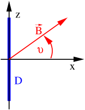
Figure 1: Coordinate system used in the simulations.

Since we are going to investigate the influence on the relative orientation of the magnetic field with respect to the easy axis of the SMM, we define the coordinate system as shown in Fig. 1. The magnetic easy axis is parallel to the $z$-axis, whereas the field vector lies in the $xz$-plane with an inclination of $\vartheta$ with the positive $x$-axis.

2.2 Equilibrium thermodynamics

Here and throughout the article we tacitly assume that the applied magnetic fields and the investigated temperatures do not violate the ranges of applicability of the giant spin models (2.1) and (2.1).

Equilibrium thermodynamic observables can be obtained from the Gibbs potential $G(T,\vec{B})$

$$G(T,\vec{B}) = -k_{B}T\ \text{log}\left[Z(T,\vec{B})\right]\ ,$$ (6)

where $Z(T,\vec{B})$ denotes the partition function. Entropy as well as magnetization are first derivatives of $G(T,\vec{B})$, i.e.

$${\mathcal{S}}(T,\vec{B}) = -\frac{\partial\,{}}{\partial\,{T}}\;\,G(T,\vec{B})\ ,$$ (7)

$$\vec{{\mathcal{M}}}(T,\vec{B}) = -\frac{\partial\,{}}{\partial\,{\vec{B}}}\;\,G(T,\vec{B})\ .$$ (8)

2.3 Non-equilibrium thermodynamics

The infinitesimal work $\delta W$ is defined by the variation of the magnetization

$$\delta W = \vec{B}\cdot\text{d}\vec{\mathcal{M}}\ .$$ (9)

Since this term is complicated to evaluate we use the following relation:

$$\oint\text{d}\left(\vec{\mathcal{M}}\cdot\vec{B}\right)=0 = \oint\vec{B}\cdot\text{d}\vec{\mathcal{M}}+\oint\vec{\mathcal{M}}\cdot\text{d}\vec{B}$$ (10)

$$\Rightarrow\;\Delta W = -\oint\vec{\mathcal{M}}\cdot\text{d}\vec{B}\>.$$ (11)

The magnetization $\vec{\mathcal{M}}$ can be obtained from the time-dependent density matrix. For the time evolution of the density matrix we employ

$$\frac{d}{dt}\;\!\hbox{}\mathop{\vphantom{\rho}\smash{\rho}}\limits_{\sim}\hbox{}\!\left(t\right) = -i\left[\!\hbox{}\mathop{\vphantom{H}\smash{H}}\limits_{\sim}\hbox{}\!,\!\hbox{}\mathop{\vphantom{\rho}\smash{\rho}}\limits_{\sim}\hbox{}\!\left(t\right)\right]+c\cdot\lambda\left(\!\hbox{}\mathop{\vphantom{\rho}\smash{\rho}}\limits_{\sim}\!{}^{(\text{eq})}(T,\vec{B})-\!\hbox{}\mathop{\vphantom{\rho}\smash{\rho}}\limits_{\sim}\hbox{}\!(t)\right)\ ,$$ (12)

with

$$\!\hbox{}\mathop{\vphantom{\rho}\smash{\rho}}\limits_{\sim}\!{}^{(\text{eq})}(T,\vec{B}) = \frac{1}{Z(T,\vec{B})}\sum_{n}\left|n\right\rangle e^{-\beta E_{n}}\left\langle n\right|\ ,$$ (13)

where $\beta=(k_{B}T)^{-1}$. $E_{n}$ and $\left|n\right\rangle$ denote the eigenvalues and the corresponding eigenvectors of the Hamiltonian. The factor $c$ depends on the nature of the current stroke in the process. For an isothermal process $c=1$, for an adiabatic (or isolated) process $c=0$. The factor $\lambda$ denotes the coupling strength of the system to one of the heat reservoirs and can in principle be different for each heat bath.

The mean magnetization can easily be calculated from the density matrix:

$$\vec{\mathcal{M}}\left(t\right) = -g\,\mu_{B}\,\text{Tr}\left\{\!\hbox{}\mathop{\vphantom{\vec{S}}\smash{\vec{S}}}\limits_{\sim}\hbox{}\!\!\hbox{}\mathop{\vphantom{\rho}\smash{\rho}}\limits_{\sim}\hbox{}\!\left(t\right)\right\}\;.$$ (14)

For the mean work $\Delta W$ done on or by the system during one stroke in the time interval $\left[t_{0}\>,\>t_{1}\right]$ one finds with (11)

$$\Delta W =- \int_{t_{0}}^{t_{1}}\vec{\mathcal{M}}\left(t\right)\cdot\dot{\vec{B}}\left(t\right)\text{d}t\ .$$ (15)

The during this process absorbed or emitted amount of heat $\Delta Q$ can be obtained from the change of the mean energy $\left\langle\!\hbox{}\mathop{\vphantom{H}\smash{H}}\limits_{\sim}\hbox{}\!\right\rangle$ of the system via the rules of thermodynamics:

$$\left\langle\!\hbox{}\mathop{\vphantom{H}\smash{H}}\limits_{\sim}\hbox{}\!\right\rangle\left(t\right) = \text{Tr}\left\{\!\hbox{}\mathop{\vphantom{H}\smash{H}}\limits_{\sim}\hbox{}\!\left(t\right)\!\hbox{}\mathop{\vphantom{\rho}\smash{\rho}}\limits_{\sim}\hbox{}\!\left(t\right)\right\}\ ,$$ (16)

$$\Delta\left\langle\!\hbox{}\mathop{\vphantom{H}\smash{H}}\limits_{\sim}\hbox{}\!\right\rangle = \left\langle\!\hbox{}\mathop{\vphantom{H}\smash{H}}\limits_{\sim}\hbox{}\!\right\rangle\left(t_{1}\right)-\left\langle\!\hbox{}\mathop{\vphantom{H}\smash{H}}\limits_{\sim}\hbox{}\!\right\rangle\left(t_{0}\right)\ =\;\Delta Q+\Delta W\;.$$ (17)

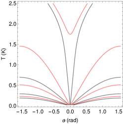
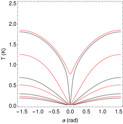
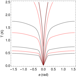
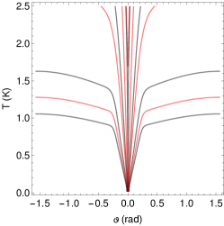
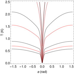
Figure 2: Isentropes of Mn₁₂ (left column) and Fe₈ (right column) for $B=0.1$ T, $B=1$ T, and $B=2$ T from top to bottom. Contours are drawn at entropy values $\mathcal{S}/k_{B}$ of $10^{-5}$, $10^{-4}$, $10^{-3}$, $0.032$, $0.1$, $0.4$, $0.68$, and $0.7$.

3 Quasi-static MCE

Quasi-static (equilibrium) MCE investigates the thermodynamic functions (7) & (8) as given by (e.g.) the canonical ensemble. Of special interest are the isentropes, i.e. curves of constant entropy, whose slopes are the so-called cooling rates as well as the isothermal entropy changes – both figures of merit for MCE materials. Figure 2 shows the isentropes of Mn₁₂ (left column) and Fe₈ (right column) for $B=0.1$ T, $B=1$ T, and $B=2$ T from top to bottom. Since both systems are modeled with rather similar Hamiltonians, the graphs for these two SMMs do look very similar. The behavior can be rationalized as follows. For a given and not too large magnitude of the external magnetic field the energy spectrum resembles a tilted parabola for $\vartheta=\pi/2$ (l.h.s. of Fig. 3). In particular, the ground state is not degenerate. This situation changes towards $\vartheta=0$ (r.h.s. of Fig. 3), where the two ground state levels are virtually degenerate. This means that all isentropes with $\mathcal{S}/k_{B}\leq\log 2$ head towards absolute zero at $\vartheta=0$. In addition, the top panels of Fig. 2 display isentropes with $\mathcal{S}/k_{B}=0.7>\log 2$ that only exhibit local minima at $\vartheta=0$. All plots are symmetric about $\vartheta=0$.

The cooling rate (slope of isentropes) assumes very large values close to $\vartheta=0$. This trend increases with increasing magnitude of the applied field. Therefore, large temperature variations should be achievable with only mild rotations in particular for stronger fields.

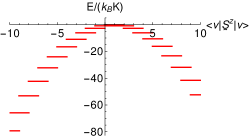
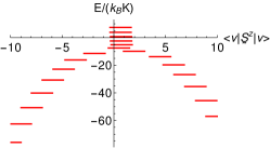
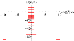
Figure 3: Energy eigenvalues vs. magnetization along $z$-direction for Mn₁₂ at $B=1$ T and $\vartheta=\pi/2$ (left), $\vartheta=\pi/4$ (middle), and $\vartheta=0$ (right).

The isothermal entropy change on the other hand is rather bounded since more than a twofold degeneracy of levels is not achievable in the physically permitted temperature and field ranges of the model. This leads to the characteristic curves displayed in Fig. 4. Shown is the negative entropy difference between final and initial orientation, i.e.

$$-\Delta{\mathcal{S}} = -\big{(}{\mathcal{S}}(T,B,\vartheta_{f})-{\mathcal{S}}(T,B,\vartheta_{i})\big{)}\ .$$ (18)

The initial angle is always taken as $\vartheta_{i}=0$. The colors of the three curves in each panel correspond to the three chosen final angles $\vartheta_{f}$ displayed above the panels.

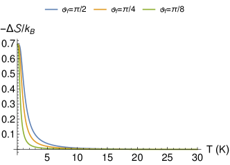
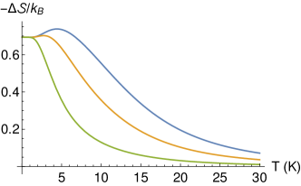
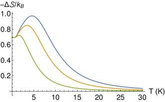
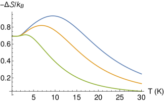
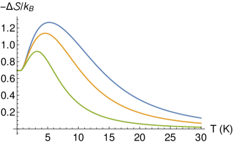
Figure 4: Isothermal entropy changes of Mn₁₂ (left column) and Fe₈ (right column) for $B=0.1$ T, $B=1$ T, and $B=2$ T from top to bottom. The rotation is performed from the initial angle $\vartheta_{i}=0$ to the final angles $\vartheta_{f}$ provided at the top.

As one notices in all panels of Fig. 4 the isothermal entropy changes head for $\mathcal{S}/k_{B}=\log 2\approx 0.68$ at low temperatures. This is a result of the twofold degeneracy at $\vartheta_{i}=0$ and the vanishingly small entropy at all other angles $\vartheta_{f}\neq 0$. For elevated temperatures the entropy change rises a bit since then also higher lying levels are thermally populated. But due to the restricted number of levels, which are separated by gaps of the order of the anisotropy, this effect is small, albeit more pronounced for stronger external fields. The biggest entropy changes can be achieved by a rotation of $\Delta\vartheta=\pi/2$ from the direction perpendicular to the easy axis into the direction of the easy axis.

4 Realistic Carnot processes

A discussion of the magnetocaloric properties as in section 3 or many publications of the field rests on the assumption of thermal equilibrium, i.e. on idealized quasi-static processes. However, a realistic cooling experiment or Carnot process is executed on short time scales of e.g. minutes [6] or shorter. Whether the system stays close to equilibrium depends on its typical relaxation times. In addition, especially for small quantum systems, it is not granted that the isolated parts of the processes, where no thermal contact is established, are indeed adiabatic. They may as well be unitary which is not the same. We do not want to get into this very complicated discussion and therefore assume that the isolated steps of our processes are described by a unitary time evolution. This assumption appears further justified since we investigate only fast processes in the following. Investigations of slower processes and processes other than Carnot are postponed to future investigations.

The Carnot process consists of two isothermal (strokes II and IV) and two isolated processes (strokes I and III). The time evolution of the medium, in our case a single Mn₁₂ SMM, is modeled via the time evolution of its density matrix according to (12). Although the cycle time $\tau_{\text{c}}$ is in reality only limited by the relaxation during the isothermal strokes, we choose for the sake of simplicity for all four strokes the same time duration. We choose $T_{\text{h}}=0.65~{}\text{K}$ as the temperature of the hot reservoir and $T_{\text{c}}=0.5~{}\text{K}$ as the temperature of the cold reservoir, respectively. For the coupling constant $\lambda$ we choose $\lambda_{\text{h}}=\lambda_{\text{c}}=10^{-1}~{}\text{ps}^{-1}$. Smaller values of $\lambda$ simply lead to a shift to lower operating frequencies $f=\tau_{\text{c}}^{-1}$ and a rescaling of the observed power. Since we investigate the Carnot process in the realization as a refrigerator important quantities of interest are the cooling power $P$ and the efficiency $\epsilon$:

$$P = \frac{Q_{\text{c}}}{\tau_{\text{c}}}\;,$$ (19)

$$\epsilon = \frac{Q_{\text{c}}}{W}\;,$$ (20)

where $Q_{\text{c}}$ is the amount of heat taken from the cold reservoir and $W$ is the amount of work absorbed by the system during one complete cycle.

The time dependent angle $\vartheta(t)$ and the behavior of the coupling constant $c\cdot\lambda$ is exemplarily shown in Fig. 5 for a cycle time of $\tau_{\text{c}}=20~{}\text{ns}$. Figure Fig. 5 also shows the process in the corresponding $T$-$\vartheta$-diagram.

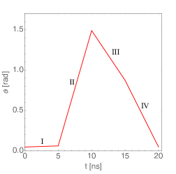
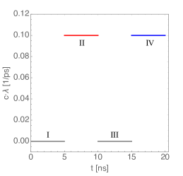
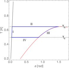
Figure 5: Exemplaric time dependence of the angle $\vartheta(t)$ (left hand side) and of the coupling constant $c\cdot\lambda$ (middle). The coupling to the hot reservoir $\lambda_{\text{h}}$ is shown in red, the coupling to the cold reservoir $\lambda_{\text{c}}$ is shown in blue. The right hand side shows an equilibrium, i.e. fully relaxed Carnot process in the $T$-$\vartheta$-diagram.

During the beginning of stroke I the system is in thermal equilibrium with the cold heat reservoir at temperature $T_{\text{c}}$. The system is then decoupled from the heat reservoir and the angle $\vartheta$ is changed with constant angular velocity from $\vartheta_{0}$ to $\vartheta_{1}$ (compare stroke I in Fig. 5). Since the system evolves isolated during this stroke there is no heat exchanged with the reservoirs. The work can therefore be calculated via (17).

During stroke II the coupling to the hot heat reservoir is switched on while the angle $\vartheta$ is further increased to $\vartheta_{2}$ with a constant (but different to the previous step) velocity (compare stroke II in Fig. 5). The system relaxes during this stroke towards thermal equilibrium with the hot heat reservoir, but depending on the time of contact with the bath, equilibrium is not necessarily reached. Since this stroke is isothermal the work must be calculated via (15). The amount of heat $Q_{\text{h}}$ exchanged with the hot heat reservoir can then be calculated via (17).

For stroke III the system is again decoupled from the heat reservoir and the angle $\vartheta$ is decreased with another constant velocity from $\vartheta_{2}$ to $\vartheta_{3}$ (compare stroke III in Fig. 5). Because this stroke is again isolated and there is again no heat exchange with any of the heat reservoirs the work can be calculated directly from (17).

During the last stroke IV the system is coupled to the cold heat reservoir at temperature $T_{\text{c}}$ while the angle $\vartheta$ is decreased with another constant velocity until the initial angle $\vartheta_{0}$ is reached and the cycle is complete (compare stroke IV in Fig. 5). The system evolves towards thermal equilibrium with the cold heat reservoir as much as possible during contact time. Since this stroke is again isothermal the work must be calculated via (15). The amount of heat $Q_{\text{c}}$ exchanged with the cold heat reservoir can then be calculated from (17).

The observables presented in the following parts are evaluated after the system has been driven through sufficiently many cycles in order to reach a steady state.

4.1 Dependence of power and operating frequencies on the amplitude of $\vec{B}(t)$

At first we investigate the influence of the amplitude $B_{0}$ of the magnetic field $\vec{B}(t)$ on the maximum cooling power $P$, the optimal operating frequency $f_{\text{opt}}$, the efficiency $\epsilon_{\text{opt}}$ as well as on the maximum operating frequency $f_{\text{max}}$. Here the optimal operating frequency $f_{\text{opt}}$ denotes the operating frequency and $\epsilon_{\text{opt}}$ the efficiency at maximum cooling power. The maximum operating frequency $f_{\text{max}}$ is the maximal frequency for which the Carnot cycle works as a refrigerator delivering heat from the cold heat reservoir to the hot one by consuming work. The results of our simulations are shown in Fig. 6. The angles $\vartheta_{0}$ to $\vartheta_{3}$ are chosen such that the process always operates between the two isentropes $\mathcal{S}_{\text{max}}/k_{B}=0.68$ and $\mathcal{S}_{\text{min}}/k_{B}=0.032$ and therefore with a fixed $\Delta\mathcal{S}/k_{B}=0.648$.

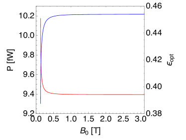
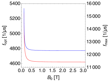
Figure 6: Dependence of the maximum cooling power $P$ and corresponding efficiency $\epsilon_{\text{opt}}$ (left hand side) and the optimal and maximal operating frequency $f$ (right hand side) on the amplitude of the magnetic field $B_{0}$. The curves belonging to the left axis are shown in red, the curves belonging to the right axis are shown in blue. Different scales are used.

The minimal possible amplitude $B_{0}$ that can satisfy $\mathcal{S}_{\text{min}}$ and $\mathcal{S}_{\text{max}}$ at the given temperatures of the heat reservoirs is $B_{0}=0.128~{}\text{T}$. As one can deduce from Fig. 6, $P$, $f_{\text{opt}}$ and $f_{\text{max}}$ are maximal for this amplitude. Only the efficiency at maximum power $\epsilon_{\text{opt}}$ is minimal. When one increases the amplitude $B_{0}$, $P$ decreases by $7.66\%$ until the amplitude $B_{0}$ reaches a threshold value of about $0.5~{}\text{T}$. The optimal operating frequency $f_{\text{opt}}$ decreases in the same time by $12.45\%$ and $f_{\text{max}}$ decreases by even $21.17\%$. The efficiency on the other hand increases by $17.15\%$. For larger values of $B_{0}$ all observed quantities become independent of $B_{0}$.

For the hot and cold temperatures $T_{\text{c}}$ and $T_{\text{h}}$, respectively, chosen in our example, one also deduces from Fig. 2 that with increasing field strength $B_{0}$ the maximum rotation angle decreases. Therefore, for large amplitudes $B_{0}$ only very small rotations are necessary.

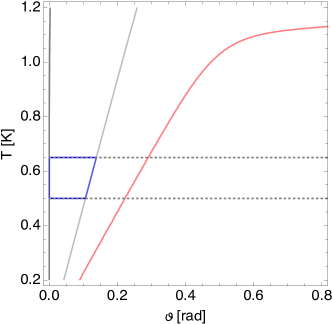
Figure 7: Exemplaric depiction of the Carnot cycle in the $T$-$\vartheta$-diagram. The isentrope $\mathcal{S}_{\text{max}}$ (black line) is fixed at $\mathcal{S}/k_{B}=0.6931$ while the isentrope $\mathcal{S}_{\text{min}}$ (gray line) is varied between black line and red curve to achieve different $\Delta\mathcal{S}$. The temperatures of the two heat reservoirs are marked by dotted gray lines. A Carnot cycle is depicted in blue.

4.2 Dependence of power and operating frequencies on $\Delta\mathcal{S}$

The quasi-static solution of the Carnot process yields a linear dependence between the heat extracted from the cold heat reservoir $\Delta Q_{\text{c}}$ and the entropy difference $\Delta\mathcal{S}$ between the two isentropes $\mathcal{S}_{\text{min}}$ and $\mathcal{S}_{\text{max}}$ of the process:

$$\Delta Q_{\text{c}} = T_{\text{c}}\cdot\Delta\mathcal{S}\;.$$ (21)

Thus a large value of $\Delta\mathcal{S}$ is intended to maximize the cooling per cycle. To investigate if this still holds for the dynamic process we investigate again the maximum cooling power $P$ and the corresponding efficiency at maximum cooling power $\epsilon_{\text{opt}}$ as well as the operating frequencies $f_{\text{opt}}$ and $f_{\text{max}}$. The amplitude $B_{0}$ of the applied magnetic field is fixed at $B_{0}=1~{}\text{T}$. We also fix the isentrope $\mathcal{S}_{\text{max}}$ to a value that is very close to the maximal possible value. We use $\mathcal{S}_{\text{max}}=0.6931~{}k_{B}$. The other isentrope $\mathcal{S}_{\text{min}}$ is varied to achieve different $\Delta\mathcal{S}$. This is exemplarily shown in Fig. 7.

The results of our simulations are shown in Fig. 8. As one can see from the left hand side of Fig. 8 the maximum cooling power $P$ grows almost linearly with $\Delta\mathcal{S}$ (red curve). But there is a significant loss of $P$ when $\Delta\mathcal{S}$ gets larger than $\Delta\mathcal{S}_{\text{opt}}=0.668~{}k_{B}$ (that is $96.44\%$ of the maximum value of $\Delta\mathcal{S}$). This loss is about almost $25\%$ when the cycle is operated at maximum $\Delta\mathcal{S}$ instead of $\Delta\mathcal{S}_{\text{opt}}$. In contrast to the quasi-static case the largest $\Delta\mathcal{S}$ does not yield the maximum performance.

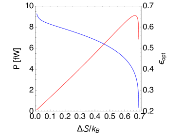
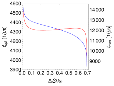
Figure 8: Dependence of the maximum cooling power $P$ and corresponding efficiency $\epsilon$ (left hand side) and the optimal and maximal operating frequency $f$ (right hand side) on the value of $\Delta\mathcal{S}$. The curves belonging to the left axis are shown in red, the curves belonging to the right axis are shown in blue. Different scales are used.

The efficiency $\epsilon_{\text{opt}}$ at maximum power decreases monotonically with growing $\Delta\mathcal{S}$ (blue curve in Fig. 8 l.h.s.), and the slope is larger for small as well as large values of $\Delta\mathcal{S}$. The same is true for the maximum operating frequency $f_{\text{max}}$ (compare blue curve in Fig. 8 r.h.s.). The optimal operating frequency $f_{\text{opt}}$, red curve in Fig. 8 r.h.s., behaves differently, since it has a local minimum at $\Delta\mathcal{S}=0.222~{}k_{B}$ ($32.1\%$ of the maximum $\Delta\mathcal{S}$) and a local maximum at $\Delta\mathcal{S}=0.570~{}k_{B}$ ($82.36\%$ of the maximum $\Delta\mathcal{S}$).

5 Summary and outlook

In this article we report investigations of the rotational magnetocaloric effect using single molecule magnets. We can conclude that the effect is present and may be used in cases where quick field changes, that are possible using mechanical rotations, are necessary. The isothermal entropy change, on the other hand, is limited since degeneracies larger than two do not arise and thus the entropy does not grow much above $\mathcal{S}/k_{B}\approx\log 2$.

A description of the Carnot process as a realistic time-dependent non-equilibrium process – using a simplified dynamics – reveals that for SMMs a threshold field amplitude exists above which the characteristic figures do not change any more. In addition and in contrast to the quasi-static case the largest $\Delta\mathcal{S}$ does not yield the maximum performance. Instead the maximum cooling power is achieved with an optimal value for $\Delta\mathcal{S}$ of only about 96 % of the maximum possible value.

In future investigations slow processes shall be studied, where the interaction with the heat bath includes the relevant phonon degrees of freedom in order to take the phonon bottleneck into account [28, 29, 30, 31, 32].

References

- Giauque and MacDougall [1933] W. F. Giauque, D. MacDougall, Attainment of Temperatures below Absolute by Demagnetization of Gd2(SO4)8H2O, Phys. Rev. 43 (1933) 768, URL https://link.aps.org/doi/10.1103/PhysRev.43.768.
- Pecharsky and Gschneidner [1999] V. K. Pecharsky, K. A. Gschneidner, Magnetocaloric effect and magnetic refrigeration, J. Magn. Magn. Mater. 200 (1999) 44–56, URL http://www.sciencedirect.com/science/article/pii/S0304885399003972.
- Waldmann et al. [2002] O. Waldmann, R. Koch, S. Schromm, P. Müller, I. Bernt, R. W. Saalfrank, Butterfly hysteresis loop at nonzero bias field in antiferromagnetic molecular rings: Cooling by adiabatic magnetization, Phys. Rev. Lett. 89 (2002) 246401.
- Evangelisti et al. [2006] M. Evangelisti, F. Luis, L. J. de Jongh, M. Affronte, Magnetothermal properties of molecule-based materials, J. Mater. Chem. 16 (2006) 2534–2549, URL http://dx.doi.org/10.1039/B603738K.
- Gomez et al. [2013] J. R. Gomez, R. F. Garcia, A. D. M. Catoira, M. R. Gomez, Magnetocaloric effect: A review of the thermodynamic cycles in magnetic refrigeration, Renewable and Sustainable Energy Reviews 17 (2013) 74 – 82, URL http://www.sciencedirect.com/science/article/pii/S136403211200528X.
- Sharples et al. [2014] J. W. Sharples, D. Collison, E. J. L. McInnes, J. Schnack, E. Palacios, M. Evangelisti, Quantum signatures of a molecular nanomagnet in direct magnetocaloric measurements, Nat. Commun. 5 (2014) 5321, URL http://dx.doi.org/10.1038/ncomms6321.
- Boeije et al. [2016] M. F. J. Boeije, P. Roy, F. Guillou, H. Yibole, X. F. Miao, L. Caron, D. Banerjee, N. H. van Dijk, R. A. de Groot, E. Brück, Efficient Room-Temperature Cooling with Magnets, Chem. Mater. 28 (14) (2016) 4901–4905, URL https://doi.org/10.1021/acs.chemmater.6b00518.
- Smith [2013] A. Smith, Who discovered the magnetocaloric effect?, Eur. Phys. J. H 38 (2013) 507–517, URL http://dx.doi.org/10.1140/epjh/e2013-40001-9.
- Trung et al. [2010] N. T. Trung, L. Zhang, L. Caron, K. H. J. Buschow, E. Brück, Giant magnetocaloric effects by tailoring the phase transitions, Appl. Phys. Lett. 96 (17) (2010) 172504, URL https://doi.org/10.1063/1.3399773.
- Sandeman [2012] K. G. Sandeman, Magnetocaloric materials: The search for new systems, Scripta Materialia 67 (2012) 566 – 571, URL http://www.sciencedirect.com/science/article/pii/S1359646212001595.
- Baniodeh et al. [2018] A. Baniodeh, N. Magnani, Y. Lan, G. Buth, C. E. Anson, J. Richter, M. Affronte, J. Schnack, A. K. Powell, High spin cycles: topping the spin record for a single molecule verging on quantum criticality, npj Quantum Materials 3 (2018) 10, URL https://doi.org/10.1038/s41535-018-0082-7.
- Evangelisti and Brechin [2010] M. Evangelisti, E. K. Brechin, Recipes for enhanced molecular cooling, Dalton Trans. 39 (2010) 4672–4676, URL http://dx.doi.org/10.1039/B926030G.
- Garlatti et al. [2013] E. Garlatti, S. Carretta, J. Schnack, G. Amoretti, P. Santini, Theoretical design of molecular nanomagnets for magnetic refrigeration, Appl. Phys. Lett. 103 (20) 202410, URL http://scitation.aip.org/content/aip/journal/apl/103/20/10.1063/1.4830002.
- Evangelisti et al. [2014] M. Evangelisti, G. Lorusso, E. Palacios, Comment on “Theoretical design of molecular nanomagnets for magnetic refrigeration” [Appl. Phys. Lett. 103, 202410 (2013)], Applied Physics Letters 105 (4) 046101, URL http://scitation.aip.org/content/aip/journal/apl/105/4/10.1063/1.4891336.
- Garlatti et al. [2014] E. Garlatti, S. Carretta, J. Schnack, G. Amoretti, P. Santini, Response to Comment on Theoretical design of molecular nanomagnets for magnetic refrigeration [Appl. Phys. Lett. 105, 046101 (2014)], Applied Physics Letters 105 (4) 046102, URL http://scitation.aip.org/content/aip/journal/apl/105/4/10.1063/1.4891337.
- Lorusso et al. [2016] G. Lorusso, O. Roubeau, M. Evangelisti, Rotating Magnetocaloric Effect in an Anisotropic Molecular Dimer, Angew. Chem. Int. Ed. 55 (2016) 3360–3363, URL http://dx.doi.org/10.1002/anie.201510468.
- Konieczny et al. [2017] P. Konieczny, R. Pełka, D. Czernia, R. Podgajny, Rotating Magnetocaloric Effect in an Anisotropic Two-Dimensional CuII[WV(CN)8]3 - Molecular Magnet with Topological Phase Transition: Experiment and Theory, Inorganic Chemistry 56 (19) (2017) 11971–11980, URL http://dx.doi.org/10.1021/acs.inorgchem.7b01930, pMID: 28915020.
- Torres et al. [2000] F. Torres, J. M. Hernandez, X. Bohigas, J. Tejada, Giant and time-dependent magnetocaloric effect in high-spin molecular magnets, Appl. Phys. Lett. 77 (2000) 3248–3250, URL http://dx.doi.org/10.1063/1.1325393.
- Zhang et al. [2001] X. X. Zhang, H. L. Wei, Z. Q. Zhang, L. Zhang, Anisotropic Magnetocaloric Effect in Nanostructured Magnetic Clusters, Phys. Rev. Lett. 87 (2001) 157203, URL https://link.aps.org/doi/10.1103/PhysRevLett.87.157203.
- Tkáč et al. [2017] V. Tkáč, R. Tarasenko, A. Orendáčová, M. Orendáč, V. Sechovský, A. Feher, Magnetocaloric effect and slow magnetic relaxation in CsGd(MoO4)2 induced by crystal-field anisotropy, Physica B: Condensed Matter (2017) in press,URL http://www.sciencedirect.com/science/article/pii/S0921452617304982.
- Tarasenko et al. [2018] R. Tarasenko, V. Tkáč, A. Orendáčová, M. Orendáč, A. Feher, Experimental study of the rotational magnetocaloric effect in KTm(MoO4)2, Physica B: Condensed Matter 538 (2018) 116 – 119, URL http://www.sciencedirect.com/science/article/pii/S0921452618302199.
- Sessoli et al. [1993] R. Sessoli, D. Gatteschi, A. Caneschi, M. A. Novak, Magnetic bistability in a metal-ion cluster, Nature 365 (1993) 141–143, URL http://dx.doi.org/10.1038/365141a0.
- Friedman et al. [1996] J. R. Friedman, M. P. Sarachik, J. Tejada, R. Ziolo, Macroscopic Measurement of Resonant Magnetization Tunneling in High-Spin Molecules, Phys. Rev. Lett. 76 (1996) 3830–3833, URL https://link.aps.org/doi/10.1103/PhysRevLett.76.3830.
- Thomas et al. [1996] L. Thomas, F. Lionti, R. Ballou, D. Gatteschi, R. Sessoli, B. Barbara, Macroscopic quantum tunnelling of magnetization in a single crystal of nanomagnets, Nature 383 (1996) 145, URL http://dx.doi.org/10.1038/383145a0.
- Wernsdorfer and Sessoli [1999] W. Wernsdorfer, R. Sessoli, Quantum Phase Interference and Parity Effects in Magnetic Molecular Clusters, Science 284 (1999) 133–135, URL http://www.sciencemag.org/content/284/5411/133.abstract.
- Barra et al. [2000] A. L. Barra, D. Gatteschi, R. Sessoli, High-Frequency EPR Spectra of [Fe8O2(OH)12(tacn)6]Br8: A Critical Appraisal of the Barrier for the Reorientation of the Magnetization in Single-Molecule Magnets, Chem. Eur. J 6 (2000) 1608–1614, URL http://dx.doi.org/10.1002/(SICI)1521-3765(20000502)6:9<1608::AID-CHEM1608>3.0.CO;2-8.
- Barco et al. [2005] E. d. Barco, A. D. Kent, S. Hill, J. M. North, N. S. Dalal, E. M. Rumberger, D. N. Hendrickson, N. Chakov, G. Christou, Magnetic Quantum Tunneling in the Single-Molecule Magnet Mn12-Acetate, J. Low Temp. Phys. 140 (2005) 119–174, URL https://doi.org/10.1007/s10909-005-6016-3.
- Chiorescu et al. [2000] I. Chiorescu, W. Wernsdorfer, A. Müller, H. Bögge, B. Barbara, Butterfly hysteresis loop and dissipative spin reversal in the , V15 molecular complex, Phys. Rev. Lett. 84 (2000) 3454–3457, URL http://link.aps.org/doi/10.1103/PhysRevLett.84.3454.
- Santini et al. [2005] P. Santini, S. Carretta, E. Liviotti, G. Amoretti, P. Carretta, M. Filibian, A. Lascialfari, E. Micotti, NMR as a probe of the relaxation of the magnetization in magnetic molecules, Phys. Rev. Lett. 94 (2005) 077203, URL http://link.aps.org/doi/10.1103/PhysRevLett.94.077203.
- Garanin [2007] D. A. Garanin, Towards a microscopic understanding of the phonon bottleneck, Phys. Rev. B 75, URL http://link.aps.org/abstract/PRB/v75/e094409.
- Carretta et al. [2008] S. Carretta, T. Guidi, P. Santini, G. Amoretti, O. Pieper, B. Lake, J. van Slageren, F. E. Hallak, W. Wernsdorfer, H. Mutka, M. Russina, C. J. Milios, E. K. Brechin, Breakdown of the Giant Spin Model in the Magnetic Relaxation of the Mn6 Nanomagnets, Phys. Rev. Lett. 100 (2008) 157203, URL http://link.aps.org/abstract/PRL/v100/e157203.
- Beckmann and Schnack [2017] C. Beckmann, J. Schnack, Investigation of thermalization in giant-spin models by different Lindblad schemes, J. Magn. Magn. Mater. 437 (2017) 7 – 11, URL http://www.sciencedirect.com/science/article/pii/S0304885316332139.