Adaptive MPC for Iterative Tasks

Abstract

This paper proposes an Adaptive Learning Model Predictive Control strategy for uncertain constrained linear systems performing iterative tasks. The additive uncertainty is modeled as the sum of a bounded process noise and an unknown constant offset. As new data becomes available, the proposed algorithm iteratively adapts the believed domain of the unknown offset after each iteration. An MPC strategy robust to all feasible offsets is employed in order to guarantee recursive feasibility. We show that the adaptation of the feasible offset domain reduces conservatism of the proposed strategy, compared to classical robust MPC strategies. As a result, the controller performance improves. Performance is measured in terms of following trajectories with lower associated costs at each iteration. Numerical simulations highlight the main advantages of the proposed approach.

I Introduction

Model Predictive Control (MPC) has established itself as a promising tool for dealing with constrained, and possibly uncertain, systems [1, 2, 3]. Challenges in MPC design include presence of disturbances and/or unknown model parameters. Disturbances can be handled by means of robust or chance constraints, and such methods are generally well understood [4, 5, 6, 7, 8]. In this paper, we are looking into methods for addressing the second challenge posed by model uncertainties.

If the actual model of a system is unknown, adaptive control strategies have been applied for meeting control objectives and ensuring system stability. Literature on unconstrained adaptive control is vast and not the subject of the current paper. Adaptive control for constrained systems has mainly focused on improving performance with the adapted models, while the constraints are satisfied robustly for all possible model realizations and for the worst disturbance bounds [9, 10]. In [11, 12] a Finite Impulse Response system model is considered for real time adaptation, but this can be restrictive as it is applicable only for asymptotically stable systems. In [13], a state space based Linear Parameter Varying model has been proposed for adaptive MPC with robust constraints. The method modifies the feasible set of states using set translations and scaling [14]. However, this assumes the existence of a unique stabilizing feedback gain matrix for all possible parametric uncertainties, which is potentially a harsh assumption. In [15, 16, 17], data driven approaches for learning and adapting system uncertainties are presented with predictive control algorithms, but they do not provide any guarantees of recursive feasibility or stability.

In this paper, we tackle the simple, yet insightful problem of regulating a constrained system in presence of additive model uncertainties. We use a model uncertainty adaptation algorithm inspired by [12], and extend it for systems performing an iterative task. Although control design for systems performing repetitive tasks has been studied [18, 19, 20], real-time model adaptation, while guaranteeing satisfaction of state-input constraints, have not yet been addressed thoroughly in literature.

We consider linear time invariant systems represented by a state-space model with known matrices. The system is subject to bounded additive uncertainty, which consists of: $(i)$ a zero mean process noise, that belongs to a known convex set, and $(ii)$ an unknown, but constant offset. Given an initial estimate of the offset domain, we iteratively refine it, using a set membership based method [12], as new data becomes available. In order to design an MPC controller with the unknown offset, we make sure the constraints on states and inputs are robustly satisfied for all feasible offsets at a time instant. Here a “feasible offset” is an offset belonging to the current estimation of the offset domain. As the feasible offset domain is updated with data iteratively, we obtain an iterative adaptation in the MPC algorithm. Moreover, to further improve control performance from one iteration to the next iteration, we use the Learning MPC (LMPC) framework [20] to construct the MPC terminal constraints and terminal cost.

The main contributions of this paper are summarized as:

• We introduce adaptation of additive uncertainty in a robust MPC algorithm, for Linear Time Invariant systems performing iterative tasks. We ensure recursive feasibility and robust stability of the resulting controller.

• We show that model adaptation iteratively relaxes the bounds of the imposed state/input constraints, as more data is collected over time. Due to this relaxation, the optimal control problem in a new iteration can lower the incurred cost further, thus iteratively reducing the conservatism in the algorithm.

• We demonstrate performance improvement with our adaptive algorithm, by comparing numerical simulation results to the results of [21].

This paper is organized as follows: Section II introduces the problem setup. Section III formulates the Adaptive Learning Model Predictive Control (ALMPC) algorithm basics, outlining the control policy and the solved finite horizon robust optimal control problem, which iteratively improves using LMPC strategy. We also elaborate the main idea of recursive uncertainty adaptation in this section. Properties of the proposed ALMPC algorithm are explained in Section IV, where we also prove recursive feasibility and robust stability of the control algorithm. Section V presents numerical simulations and comparisons, and Section VI concludes the paper and outlines possible future extensions.

II Problem Statement

Given an initial state $x_{S}$, we consider uncertain linear time-invariant systems of the form

$$x_{t+1}=Ax_{t}+Bu_{t}+E\theta_{a}+w_{t},\quad x_{0}=x_{S},$$ (1)

where $x_{t}\in\mathbb{R}^{n_{x}}$ is the state at time $t$, $u_{t}\in\mathbb{R}^{n_{u}}$ is the input, and $A$ and $B$ are known system matrices. At each time step $t$, the system is affected by a random process noise $w_{t}\in\mathbb{W}\subset\mathbb{R}^{n_{w}}$, which is considered to have a zero mean. In this paper, $\mathbb{W}$ is assumed to be a compact convex polytope. We also consider the presence of a constant offset $\theta_{a}\in\mathbb{R}^{p}$, which affects the state dynamics through the known matrix $E\in\mathbb{R}^{n_{x}\times p}$. We consider constraints of the form

$$Fx_{t}+Gu_{t}\leq f,$$ (2)

which must be satisfied for all uncertainty realizations $w_{t}\in\mathbb{W}$. The matrices $F\in\mathbb{R}^{n_{f}\times n_{x}}$, $G\in\mathbb{R}^{n_{f}\times n_{u}}$ and $f\in\mathbb{R}^{n_{f}}$ are assumed known. Throughout the paper, we assume that system (1) performs the same task repeatedly. Each task execution is referred to as iteration. At each $j^{\textnormal{th}}$ iteration, the performance of the $j^{\textnormal{th}}$ realized closed loop trajectory is quantified with the iteration cost

$$V^{(j)}=\sum_{t=0}^{\infty}\ell(x_{t}^{(j)},u_{t}^{(j)})$$ (3)

where $x_{t}^{(j)}$ and $u_{t}^{(j)}$ denote the realized system state and the control input at time $t$, respectively, and $\ell:\mathbb{R}^{n_{x}}\times\mathbb{R}^{n_{u}}\to\mathbb{R}_{+}$ is a positive definite stage cost.

Our goal is to design a controller that, at each iteration $j$, solves the infinite horizon robust optimal control problem:

$$\begin{array}[]{clll}V^{(j),\star}(x_{S})=\\[4.30554pt] \displaystyle\min_{u_{0}^{(j)},u_{1}^{(j)}(\cdot),\ldots}&\displaystyle\sum\limits_{t\geq 0}\ell\left(\bar{x}_{t}^{(j)},u_{t}^{(j)}\left(\bar{x}_{t}^{(j)}\right)\right)\\[4.30554pt] \text{s.t.}&x_{t+1}^{(j)}=Ax_{t}^{(j)}+Bu_{t}^{(j)}(x_{t}^{(j)})+E\theta_{a}+w_{t}^{(j)},\\[4.30554pt] &Fx_{t}^{(j)}+Gu_{t}^{(j)}\leq f,\ \forall w_{t}^{(j)}\in\mathbb{W},\\[4.30554pt] &x_{0}^{(j)}=x_{S},\ t=0,1,\ldots,\end{array}$$ (4)

where $\theta_{a}$ is the constant offset present in the system and $\bar{x}_{t}^{(j)}$ denotes the disturbance-free nominal state. Notice that (4) minimizes the nominal cost. We point out that, as system (1) is uncertain, the optimal control problem (4) consists of finding $[u_{0}^{(j)},u_{1}^{(j)}(\cdot),u_{2}^{(j)}(\cdot),\ldots]$, where $u_{t}^{(j)}:\mathbb{R}^{n_{x}}\ni x_{t}^{(j)}\mapsto u_{t}^{(j)}=u_{t}^{(j)}(x_{t}^{(j)})\in\mathbb{R}^{n_{u}}$ are state feedback policies. It is important to note that in practical applications, each iteration has a finite time duration. However, it is common in literature to adopt an infinite time formulation at each iteration, for the sake of simplicity [20], as done in this paper.

In this paper, we try to compute a solution to the infinite time optimal control problem (4), by solving a finite time constrained optimal control problem. Moreover, we assume that offset $\theta_{a}$ in (4) is not known exactly. Therefore, we propose a parameter estimation framework to refine our knowledge of $\theta_{a}$ and thus, improve controller performance. We also guarantee recursive constraint satisfaction for all possible offsets.

III Adaptive Learning MPC

We design a finite horizon MPC controller in an attempt to solve (4) for regulating (1) to the origin. The key idea is to use data to learn the unknown offset $\theta_{a}$, while exploiting the iterative nature of the problem to improve the performance at the next iteration. In particular:

1. The knowledge of the potential domain of offset $\theta_{a}$ is refined in every iteration, using a set membership based approach [12, 11], giving rise to an Adaptive MPC algorithm. Due to this uncertainty adaptation, and resulting constraint relaxation, the optimal control problem in a new iteration can lower the incurred cost further, thus iteratively reducing conservatism.

2. We combine the above uncertainty adaptation with a technique called Learning Model Predictive Control (LMPC) [20], to design an Adaptive Learning MPC (ALMPC) controller, whose performance improves iteratively by learning the terminal cost and terminal constraint in the MPC algorithm.

In the following sections, we present the detailed mathematical formulations to achieve steps $(1)$ and $(2)$.

III-A Estimating $\theta_{a}$

We characterize the knowledge of the offset $\theta_{a}$ by its domain $\Theta$, called the Feasible Parameter Set, which we estimate from previous system data. This is initially chosen as a polytope $\Theta^{(0)}$, and it is assumed that $\theta_{a}\in\Theta^{(0)}$ for all times. The set is then updated at the end of each iteration after gathering input-output data for all time steps. For the $j^{\textnormal{th}}$ iteration, the updated Feasible Parameter Set, denoted by $\Theta^{(j)}$, is given by

$$\Theta^{(j)}=\{\theta\in\mathbb{R}^{p}:x^{(i)}_{t}-Ax^{(i)}_{t-1}-Bu^{(i)}_{t-1}-E\theta\in\mathbb{W}\\ \forall i\in[0,\ldots,j-1],\forall t\geq 0\}.$$ (5)

It is clear from (5) that as iterations go on, new data is progressively added to improve the knowledge of $\Theta$, without discarding previous information. Knowledge from all previous iterations is included in $\Theta^{(j)}$. Thus, updated Feasible Parameter Sets are obtained with intersection operations on polytopes, and so $\Theta^{(j+1)}\subseteq\Theta^{(j)}$.

III-B MPC Problem

In this section, we present the proposed ALMPC algorithm.

Control Policy Approximation

We consider affine state feedback policies of the form [22, 23]

$$u^{(j)}_{t}(x_{t})=K\left(x^{(j)}_{t}-\bar{x}^{(j)}_{t}\right)+v^{(j)}_{t},$$ (6)

where $K\in\mathbb{R}^{n_{u}\times n_{x}}$ is a fixed feedback gain same for all iterations $j$. $\bar{x}^{(j)}_{t}$ is the nominal state and $v^{(j)}_{t}$ is an auxiliary control input. The parametrization (6) allows us to decouple the state dynamics (1) into a nominal state $s^{(j)}_{t}\equiv\bar{x}^{(j)}_{t}$ and an error state $e^{(j)}_{t}=x^{(j)}_{t}-s^{(j)}_{t}$, whose respective dynamics are given by

$$s^{(j)}_{t+1} =As^{(j)}_{t}+Bv_{t}^{(j)},\quad s^{(j)}_{0}=x_{S},\quad j=0,1,\ldots$$ (7a)

$$e^{(j)}_{t+1} =\Psi e^{(j)}_{t}+E\theta_{a}+w_{t},~{}e^{(j)}_{0}=0,\quad j=0,1,\ldots,$$ (7b)

where $\Psi:=(A+BK)$. Above, the state $s_{t}^{(j)}$ is uncertainty-free, while the error state contains both the process noise as well as the (unknown) offset $\theta_{a}$.

Reformulation of Constraints

The constraints (2) on states and inputs, defined in (4), can be reformulated in terms of nominal and error states using (7). Hence, substituting (7) in (4), we can derive the corresponding constraints on the nominal states as

$$Fs_{t}^{(j)}+Gv_{t}^{(j)}+(F+GK)e_{t}^{(j)}\leq f,$$ (8)

where error state $e_{t}^{(j)}$ follows the dynamics (7b). Now, we need to ensure that constraints (8) are satisfied $\forall w_{t}^{(j)}\in\mathbb{W}$, in presence of the unknown offset $\theta_{a}$. Therefore, (8) are imposed for all models in the Feasible Parameter Set, i.e. $\forall\theta\in{\Theta}^{(j)}$ and for all $t\geq 0$, in the $j^{\textnormal{th}}$ iteration. Thus, we modify considered error state dynamics (7b) as

$$e_{t+1}^{(j)}=\Psi e_{t}^{(j)}+d_{t}^{(j)},\quad e^{(j)}_{0}=0,~{}\quad j=0,1,\ldots,$$ (9)

where $d_{t}^{(j)}=\{d:d=w+E\theta,\ \forall w\in\mathbb{W},\ \forall\theta\in\Theta^{(j)}$, and ensure

$$Fs_{t}^{(j)}+Gv_{t}^{(j)}+(F+GK)e_{t}^{(j)}\leq f,\ \ \forall d_{t}^{(j)}\in\mathbb{W}\oplus E\Theta^{(j)}.$$

Tractable Reformulation

We now solve the following finite horizon robust optimal control problem at each time step $t$ of iteration $j$

$$\begin{array}[]{clll}V_{t\to t+N}^{\text{ALMPC},j}(s_{t}^{(j)})=\\[4.30554pt] \displaystyle\min_{v_{t|t}^{(j)},\ldots,v_{t+N-1|t}^{(j)}}&\displaystyle\sum\limits_{k=t}^{t+N-1}\ell\left(s_{k|t}^{(j)},v_{k|t}^{(j)}\right)+P^{(j-1)}(s_{t+N|t}^{(j)})\\[4.30554pt] \text{s.t.}&s_{k+1|t}^{(j)}=As_{k|t}^{(j)}+Bv_{k|t}^{(j)},\\[4.30554pt] &Fs_{k|t}^{(j)}+Gv_{k|t}^{(j)}\leq f-h_{s}^{(j)},\\[4.30554pt] &s_{t|t}^{(j)}=s_{t}^{(j)},\ s_{t+N|t}^{(j)}\in\mathcal{CS}^{(j-1)},\\[4.30554pt] &k=t,\ldots,t+N-1,\end{array}$$ (10)

where $h^{(j)}_{s}=\max\limits_{e_{t}\in\mathcal{E}^{(j)}}\Phi e_{t}$, $\Phi=(F+GK)$, and the set $\mathcal{E}^{(j)}$ is assumed to be the minimal robust positive invariant set for the error in (9), for iteration $j$ [23, Definition 3.4]. Terminal constraint $\mathcal{CS}^{(j-1)}$, and the terminal cost $P^{(j-1)}(\cdot)$ are discussed in details next. As $\Theta^{(j)}$ is updated using (5), the set $\mathcal{E}^{(j)}$ alters after every iteration. Therefore, the solved MPC problem (10) is adaptive in nature. Upon solving (10), the controller applies

$$u_{t}^{(j)}(x_{t}^{(j)})=K(x_{t}^{(j)}-s_{t}^{(j)})+v_{t|t}^{(j),\star}$$ (11)

to the system (1), where $v_{t|t}^{(j),\star}$ is the first input from the optimal input sequence of (10).

Now we discuss the component of Learning in this adaptive MPC algorithm, which corresponds to an iterative performance improvement, i.e. decrease of closed loop cost from iteration to iteration.

Construction of Terminal Conditions

In (10) the nominal terminal state is constrained into the control invariant safe set $\mathcal{CS}^{(j-1)}$, and the terminal cost is denoted by $P^{(j-1)}(\cdot)$. These are borrowed from Learning MPC for deterministic systems [20], whose main idea we revisit next. At iteration $j$, let the vectors

$${\bf{v}}^{(j)}~{}=~{}[v_{0}^{(j)},~{}v_{1}^{(j)},~{}...,~{}v_{t}^{(j)},~{}...],$$ (12a)

$${\bf{s}}^{(j)}~{}=~{}[s_{0}^{(j)},~{}s_{1}^{(j)},~{}...,~{}s_{t}^{(j)},~{}...],$$ (12b)

denote the nominal input and state of system (7a). To exploit the iterative nature of the control design, we define the sampled Safe Set $\mathcal{SS}^{(j)}$ at iteration $j$ as

$$\mathcal{SS}^{(j)}=\textrm{}\left\{\bigcup_{i\in M^{(j)}}\bigcup_{t=0}^{\infty}s_{t}^{(i)}\right\},$$ (13)

where $M^{(j)}\subseteq\{0,\ldots,j\}$ is the set of indices associated with successful iterations, i.e.,

$$M^{(j)}=\textrm{}\Big{\{}k\in[0,j]:\lim_{t\to\infty}s_{t}^{(k)}=0\Big{\}}.$$

In other words, $\mathcal{SS}^{(j)}$ is the collection of all nominal state trajectories up to iteration $j$ that have converged to the origin. We define the convex Safe Set as

$$\mathcal{CS}^{(j)}=\text{conv}(\mathcal{SS}^{(j)}).$$ (14)

Now, at time $t$ of the $j^{\textnormal{th}}$ iteration, the cost-to-go associated with the closed loop trajectory (12b) and input sequence (12a) is defined as

$$V_{t\rightarrow\infty}^{(j)}(s_{t}^{(j)})=~{}\sum\limits_{k=0}^{\infty}\ell(s_{t+k}^{(j)},v_{t+k}^{(j)}),$$

where $\ell(\cdot,\cdot)$ is the stage cost of problem (10). We define the barycentric function

$$P^{(j)}(s)=\begin{cases}p^{(j),*}(s)&\mbox{if }s\in\mathcal{CS}^{(j)}\\ +\infty&\mbox{else}\\ \end{cases},$$ (15)

where

$$p^{(j),*}(s)=\min_{\lambda_{t}\geq 0,\forall t\in[0,\infty)}\sum_{k=0}^{j}\sum_{t=0}^{\infty}\lambda_{t}^{(k)}V_{t\rightarrow\infty}^{(k)}(s_{t}^{(k)})$$

$$\text{s.t.}\qquad\ \sum_{k=0}^{j}\sum_{t=0}^{\infty}\lambda_{t}^{(k)}=1,\ \sum_{k=0}^{j}\sum_{t=0}^{\infty}\lambda_{t}^{(k)}s_{t}^{(k)}=s,$$

where $s_{t}^{(k)}$ is the nominal state at time $t$ of the $k^{\textnormal{th}}$ iteration, as defined in (12b). The function $P^{(j)}(\cdot)$ assigns to every point in $\mathcal{CS}^{(j)}$ the minimum cost-to-go along the trajectories in $\mathcal{CS}^{(j)}$. Therefore this choice of terminal cost in (10) guarantees that at each iteration, the iteration cost is non-increasing [20, Theorem 2].

Intuitively, the function $P^{(j)}(.)$ quantifies the performance of the closed loop trajectories in the previous iterations. This information from the previous iteration data is exploited to guarantee iterative performance improvement and therefore, the algorithm has a “learning property”.

Algorithm 1 Adaptive Learning MPC

1:Start with iteration $j$. Set $t=0$; initialize Feasible Parameter Set $\Theta^{(j)}$ and compute initial minimal robust positive invariant set $\mathcal{E}^{(j)}$ using algorithm in [23, Chapter 3].

2:Compute $v_{t|t}^{(j),\star}$ from (10) and apply $v^{(j)}_{t}=v_{t|t}^{(j),\star}$ to the system.

3:Set $t=t+1$, and return to step 2 until the end of $j^{\textnormal{th}}$ iteration.

4:At the end of $j^{\textnormal{th}}$ iteration, set the convex hull of the nominal states’ as the convex safe set, $\mathcal{CS}^{(j)}$ for next iteration [20].

5:Update $\Theta^{(j)}$ using (5). Set $j=j+1$. Return to step 1.

We formulate an optimal control problem to find a feasible trajectory which can be used to initialize the ALMPC. We make the following assumption for our system:

Assumption 1

We assume we are given an initial state and input sequence $(\mathbf{s}^{(0)},\mathbf{v}^{(0)})$ that satisfies the constraints (7a) and $Fs_{t}^{(0)}+Gv_{t}^{(0)}\leq f-\max_{e\in\mathcal{E}^{(0)}}\{\Phi e\}$ for all $t\geq 0$, where $\mathcal{E}^{(0)}$ is the minimal robust positive invariant set for (9) in the first iteration.

Remark 1

Since the system (7a) is linear and the constraints are convex, every convex combination of the trajectories in the sampled safe set $\mathcal{SS}^{(j)}$ is a feasible trajectory, which steers the system to the origin. Therefore $\mathcal{CS}^{(j)}$ is a control invariant set for (7a) [24]. This is required for proving recursive feasibility of MPC problem (10) in closed loop with controller (11) [24, Theorem 1].

Remark 2

The decoupling of the state dynamics in (7) is a linear change of coordinates, and is not necessary to implement the proposed strategy. Indeed, it is possible to reformulate the controller in the coordinate frame of system (1). In particular, using standard set theory tools [3, Chaper 10], one could tighten the constraints (2) and the terminal set $\mathcal{CS}$ (14) to guarantee robustness against all disturbance realizations.

IV Properties of Adaptation

In this section we discuss the properties and associated advantages of model uncertainty adaptation (5), namely: $(i)$ decreasing constraint tightening, and $(ii)$ convergence guarantees.

IV-A Decreased Constraint Tightening

It is evident that in (10), the constraints on the nominal state $s$ are tightened based on the size of the set $\mathcal{E}^{(j)}$. The set $\mathcal{E}^{(j)}\subset\mathbb{R}^{n_{x}}$ the minimal robust positive invariant set for the error dynamics (9) in iteration $j$, which is defined as [23, Eq. 3.23]

$$\mathcal{E}^{(j)}=\bigoplus\limits_{i=0}^{\infty}\Psi^{i}(\mathbb{W}\oplus E\Theta^{(j)}),$$ (17)

which satisfies the condition that, for all $e_{0}^{(j)}\in\mathcal{E}^{(j)}$, we have $e^{(j)}_{t}(\mathbf{w}_{t-1},{\color[rgb]{0,0,0}\theta})\in\mathcal{E}^{(j)}$ for all $\mathbf{w}_{t-1}=[w_{0},\ldots,w_{t-1}]\in\mathbb{W}$, for all $\theta\in\Theta^{(j)}$ and all $t\geq 1$.

Lemma 1

The minimal robust positive invariant set $\mathcal{E}^{(j)}$, is monotonically decreasing with respect to iterations. That is, for successive iterations of the system, it follows the property $\mathcal{E}^{(j+1)}\subseteq\mathcal{E}^{(j)}$.

Proof:

New cuts are added to the Feasible Parameter Set polytope $\Theta^{(j)}$ according to (5) to obtain $\Theta^{(j+1)}$ at the next iteration. Namely, from (5), we have that

$$\Theta^{(j+1)}=\Theta^{(j)}\cap\{\theta\in\mathbb{R}^{p}:x^{(j+1)}_{t}-Ax^{(j+1)}_{t-1}-Bu^{(j+1)}_{t-1}\\ -E\theta\in\mathbb{W},\forall t\geq 0\}.$$

Therefore, $\Theta^{(j+1)}\subseteq\Theta^{(j)}$. So from (17) we get

$$\mathcal{E}^{(j+1)}=\bigoplus\limits_{i=0}^{\infty}\Psi^{i}(\mathbb{W}\oplus E\Theta^{(j+1)})\subseteq\bigoplus\limits_{i=0}^{\infty}\Psi^{i}(\mathbb{W}\oplus E\Theta^{(j)}).$$ (18)

This shows that $\mathcal{E}^{(j+1)}\subseteq\mathcal{E}^{(j)}$, and concludes the proof. ∎

The decreasing size of the minimal robust positive invariant set $\mathcal{E}^{(j)}$, clearly reduces constraint tightening in (10) for nominal states. That indicates a less conservative algorithm as more data becomes available. Now we prove recursive feasibility of the resulting ALMPC algorithm, for which Lemma 1 is a sufficient condition along with terminal constraints given by convex safe set $\mathcal{CS}$.

Theorem 1

Now consider system (1) in closed loop with the ALMPC (10) and (11). Let Assumption 1 and (18) hold. Then ALMPC (10), (11) is feasible for all times $t\geq 0$ and all iterations $j\geq 1$.

Proof:

As shown in Lemma 1, $\mathcal{E}^{(j+1)}\subseteq\mathcal{E}^{(j)}$, this implies that

$$\max_{e\in\mathcal{E}^{(j+1)}}\Phi e\leq\max_{e\in\mathcal{E}^{(j)}}\Phi e.$$ (19)

Consequently, if a realized trajectory at iteration $j$ robustly satisfies input and state constraints,

$$Fs_{k|t}^{(j)}+Gv_{k|t}^{(j)}\leq f-h^{(j)}_{s},\ h^{(j)}_{s}=\max\limits_{\forall e_{t}\in\mathcal{E}^{(j)}}\Phi e_{t},$$ (20)

then this trajectory would also robustly satisfy state and input constraints at the next iteration

$$Fs_{k|t}^{(j+1)}+Gv_{k|t}^{(j+1)}\leq f-h^{(j+1)}_{s},\ h^{(j+1)}_{s}=\max\limits_{\forall e_{t}\in\mathcal{E}^{(j+1)}}\Phi e_{t}.$$ (21)

This implies that at each $j^{\textnormal{th}}$, iteration the first $j-1$ iterations robustly satisfy state and input constraints for system (1) and the disturbance $(\mathbb{W}\oplus E{\Theta}^{(j)})$. Therefore, using the fact from Remark 1 and [24, Theorem 1], the ALMPC is recursively feasible at each $j^{\textnormal{th}}$ iteration. ∎

IV-B Convergence Guarantees

In this section we first show that system (1) in closed loop with the controller (11), guarantees convergence to a neighborhood of the origin. Then, we show that the adaptive strategy allows at each iteration to shrink the guaranteed region of convergence around the origin.

Theorem 2

Consider system (1) in closed loop with the ALMPC (10) and (11). Let Assumption 1 hold. Then the closed-loop system (1), (11) converges asymptotically to the set $\mathcal{E}^{j}$ for every iteration $j\geq 1$ and all $w\in\mathbb{W}$, i.e $x_{t}^{(j)}\rightarrow\mathcal{E}^{(j)}$ as $t\rightarrow\infty$.

Proof:

The proof is based on [24, Theorem 1]: We have that $\lim_{t\rightarrow\infty}s_{t}^{(j)}=0,~{}\forall j\geq 1$ [24]. Finally, from the definition of $e_{t}=x_{t}^{(j)}-s_{t}^{(j)}$ we have $\lim_{t\rightarrow\infty}x_{t}^{(j)}=\lim_{t\rightarrow\infty}(s_{t}^{(j)}+e_{t}^{(j)})=\lim_{t\rightarrow\infty}e_{t}^{(j)}\in\mathcal{E}^{(j)},~{}\forall j\geq 1$, which concludes the proof. ∎

Now, from (18), we know $\mathcal{E}^{(j+1)}\subseteq\mathcal{E}^{(j)}$. Hence, the ALMPC delivers improved guarantees of the region of convergence iteratively, as a consequence of update (5).

V Simulation Results

In this section we compare the results of our ALMPC algorithm in Algorithm 1 with the Robust Learning MPC (RLMPC) presented in [21]. For numerical simulations, we apply both ALMPC and RLMPC algorithms to compute feasible solutions to the following iterative infinite horizon optimal control problem

$$\begin{array}[]{llll}&V^{(j),\star}(x_{S})=\displaystyle\min_{u_{0}^{(j)},u_{1}^{(j)}(\cdot),\ldots}\displaystyle\sum\limits_{t\geq 0}\left\|\bar{x}_{t}^{(j)}\right\|_{1}+10\left\|u_{t}^{(j)}\right\|_{1}\\[4.30554pt] &\text{s.t.}\\ &x_{t+1}^{(j)}=\begin{bmatrix}1.2&1.5\\ 0&1.3\end{bmatrix}x_{t}^{(j)}+\begin{bmatrix}0\\ 1\end{bmatrix}u_{t}^{(j)}(x_{t}^{(j)})\\ &~{}~{}~{}~{}~{}~{}~{}~{}~{}~{}~{}~{}~{}~{}~{}~{}~{}~{}~{}~{}~{}~{}~{}~{}~{}~{}~{}~{}~{}~{}~{}+\begin{bmatrix}1&0\\ 0&1\end{bmatrix}\begin{bmatrix}0.01\\ 0.05\end{bmatrix}+w_{t}^{(j)},\\[10.76385pt] &\begin{bmatrix}-10\\ -10\\ -1\end{bmatrix}\leq\begin{bmatrix}x_{t}^{(j)}\\ u_{t}^{(j)}\end{bmatrix}\leq\begin{bmatrix}10\\ 10\\ 1\end{bmatrix},\ \forall w_{t}^{(j)}\in\mathbb{W},\\[15.0694pt] &x_{0}^{(j)}=x_{S},\ t=0,1,\ldots,\end{array}$$ (22)

where $w_{t}\in\mathbb{W}=\{w\in\mathbb{R}^{2}:||w||_{\infty}\leq 0.8\}$. The initial Feasible Parameter Set is defined as

$$\Theta^{(0)}=\{\theta\in\mathbb{R}^{2}:\begin{bmatrix}-0.2\\ -0.1\\ \end{bmatrix}\leq\theta\leq\begin{bmatrix}0.2\\ 0.1\end{bmatrix}\}.$$ (23)

The true offset parameter is $\theta_{a}=[0.01,0.05]^{\top}$. The matrix $E\in\mathbb{R}^{2\times 2}$ is picked as the identity matrix. We solve the above optimization problem for arbitrarily chosen initial state $x_{S}=[-5.6,1.29]^{\top}$. The ALMPC in (10), (11), and the RLMPC [21] are implemented with a control horizon of $N=3$, and the feedback gain $K$ in (11) is chosen to be the optimal LQR gain for system (7a) with parameters $Q=I$ and $R=10$.

In the case of RLMPC, the domain set for the unknown offset is kept constant throughout as $\Theta^{(0)}$. Contrarily, the ALMPC algorithm proposed in this paper, shrinks the domain of the offset set with (5). This adaptation lowers the degree of constraint tightening over iterations due to (18).

V-A Uncertainty Adaptation in ALMPC

We illustrate the adaptation of additive uncertainty in this section. Feasible Parameter Set is adapted after every iteration according to (5) after being initialized as (23). This is seen from Fig. 1. It is clearly observed from Fig. 1 that the additive offset uncertainty is shrunk with every iteration. The true offset, which is picked solely for simulation purposes, is marked by $\star$ and is always inside the Feasible Parameter Set for all iterations. This underscores the fact that the robustification of the MPC problem (10) for all feasible offsets in the Feasible Parameter Set, also captures the dynamics with the true offset.

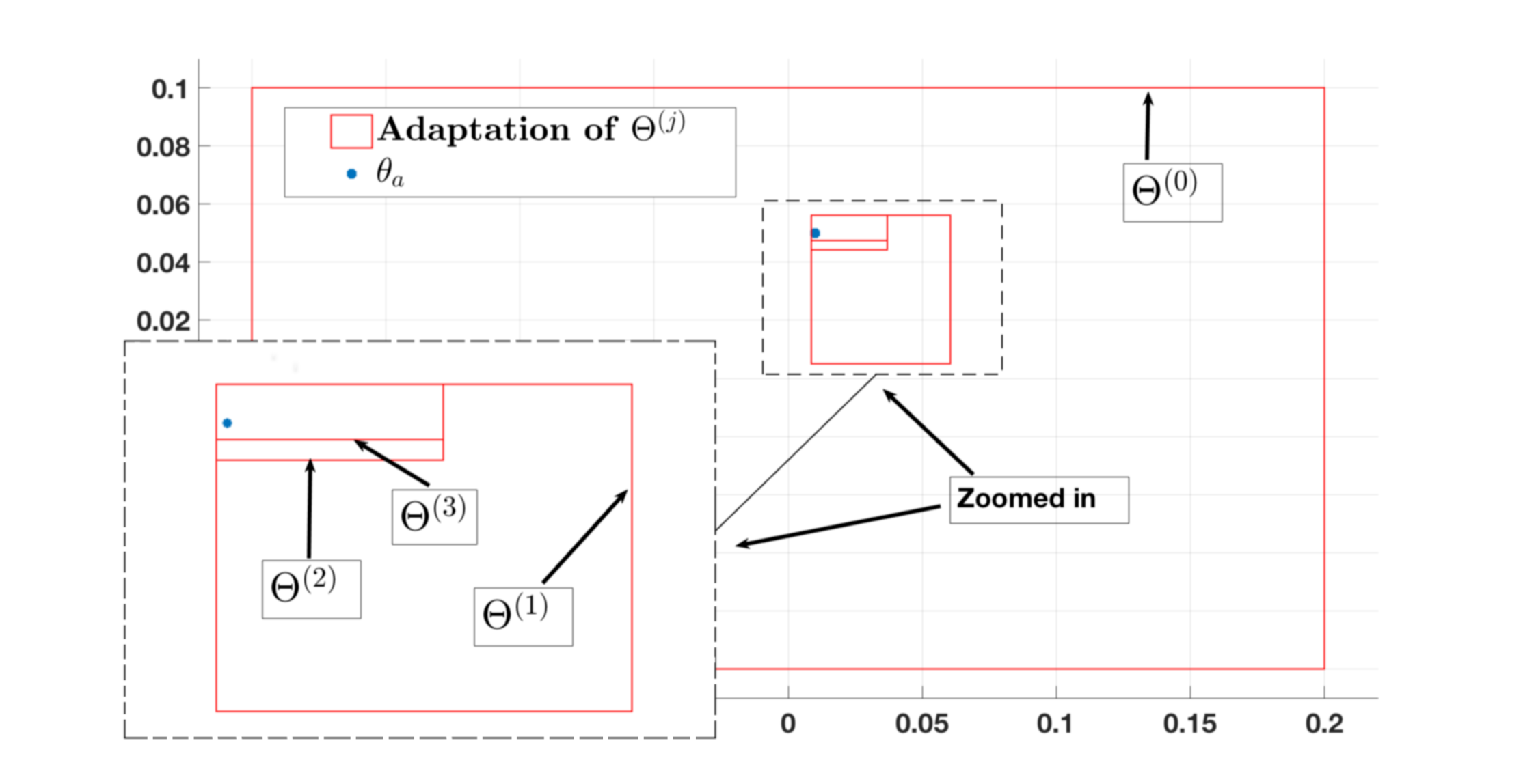
Figure 1: Adaptation of Feasible Parameter Set

As a consequence of the above uncertainty adaptation, the size of the minimal robust positive invariant set $\mathcal{E}^{(j)}$ shrinks as in (18). This is highlighted in Fig. 2. Whereas for RLMPC, the size of the minimal robust positive invariant set for dynamics (9) is constant. This keeps the same magnitude of constraint tightening throughout all iterations in (10).

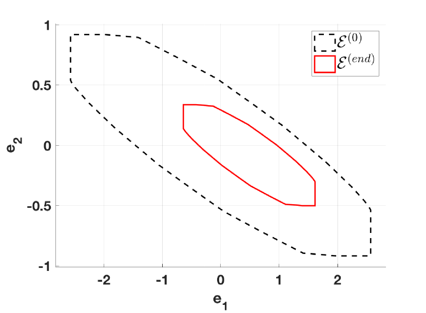
Figure 2: Adaptation of Minimal Robust Positive Invariant Set

V-B Performance Gain Over RLMPC

In this section we compare the results of the ALMPC algorithm with RLMPC [21] to illustrate the performance improvement as a result of uncertainty adaptation, and thus, minimal robust positive invariant set adaptations as shown in Fig. 1 and Fig. 2. We quantify this performance gain with two quantifiers:

• Trajectories with enhanced exploration of state space

• Lower iteration costs

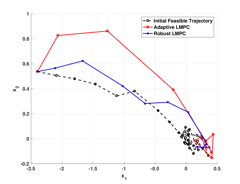
Figure 3: Trajectory Comparison after Fifth Iteration

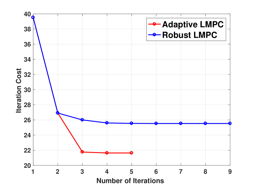
Figure 4: Iteration Cost Comparison

Fig. 3 shows the comparison of final system trajectories with both the algorithms. It is observed that the ALMPC algorithm generates a converged trajectory farther away from the initialized one, highlighting better exploration property. On the other hand, the RLMPC algorithm trajectory stays relatively closer to the initialized path, as it overestimates potential uncertainties by not adapting them.

To prove that this aforementioned exploration advantage does not come at the penalty of additional iteration costs, we compare the iteration costs of the two algorithms in Fig. 4. The ALMPC algorithm results in lower iteration costs, again proving the advantage of uncertainty adaptation.

VI Conclusion and future work

In this paper, we successfully merged an additive uncertainty adaptation methodology with the LMPC framework, to formulate the ALMPC algorithm. We proved that with every iteration, if the uncertainty is learned and thus shrunk, the amount of constraint tightening is lowered for nominal states. We have conclusively shown with numerical simulations, that the ALMPC framework, compared to RLMPC [21], explores better trajectories with lower iteration costs as uncertainty is recursively adapted. Thus, ALMPC is shown to have improved performance over RLMPC. We also proved recursive feasibility and robust stability of the ALMPC algorithm.

In future extensions of this work, we aim to solve an iterative stochastic MPC problem with model uncertainty adaptation. The inherent uncertainty adaptation algorithm in presence of constraints, can also be exploited in systems as [25, 26] for obtaining better performance. Finally, we also wish to deal with time varying uncertainties in state-space, building on the work of [27].

References

References

- [1] Manfred Morari and Jay H Lee “Model predictive control: past, present and future” In Computers & Chemical Engineering 23.4 Elsevier, 1999, pp. 667–682
- [2] David Q Mayne, James B Rawlings, Christopher V Rao and Pierre OM Scokaert “Constrained model predictive control: Stability and optimality” In Automatica 36.6 Elsevier, 2000, pp. 789–814
- [3] Francesco Borrelli, Alberto Bemporad and Manfred Morari “Predictive control for linear and hybrid systems” Cambridge University Press, 2017
- [4] D Limon, I Alvarado, T Alamo and EF Camacho “Robust tube-based MPC for tracking of constrained linear systems with additive disturbances” In Journal of Process Control 20.3 Elsevier, 2010, pp. 248–260
- [5] Mayuresh V Kothare, Venkataramanan Balakrishnan and Manfred Morari “Robust constrained model predictive control using linear matrix inequalities” In Automatica 32.10 Elsevier, 1996, pp. 1361–1379
- [6] Paul J Goulart, Eric C Kerrigan and Jan M Maciejowski “Optimization over state feedback policies for robust control with constraints” In Automatica 42.4 Elsevier, 2006, pp. 523–533
- [7] Alexander T Schwarm and Michael Nikolaou “Chance-constrained model predictive control” In AIChE Journal 45.8 Wiley Online Library, 1999, pp. 1743–1752
- [8] X. Zhang, K. Margellos, P. Goulart and J. Lygeros “Stochastic Model Predictive Control Using a Combination of Randomized and Robust Optimization” In IEEE Conference on Decision and Control (CDC), 2013
- [9] Anil Aswani, Humberto Gonzalez, S Shankar Sastry and Claire Tomlin “Provably safe and robust learning-based model predictive control” In Automatica 49.5 Elsevier, 2013, pp. 1216–1226
- [10] Anil Aswani, Patrick Bouffard and Claire Tomlin “Extensions of learning-based model predictive control for real-time application to a quadrotor helicopter” In American Control Conference (ACC), 2012, 2012, pp. 4661–4666 IEEE
- [11] M. Bujarbaruah, X. Zhang and F. Borrelli “Adaptive MPC with Chance Constraints for FIR Systems” In Accepted for IEEE-ACC, Milwaukee, WI, June 27-29, 2018
- [12] Marko Tanaskovic, Lorenzo Fagiano, Roy Smith and Manfred Morari “Adaptive receding horizon control for constrained MIMO systems” In Automatica 50.12 Elsevier, 2014, pp. 3019–3029
- [13] Matthias Lorenzen, Frank Allgöwer and Mark Cannon “Adaptive Model Predictive Control with Robust Constraint Satisfaction” In IFAC-PapersOnLine 50.1 Elsevier, 2017, pp. 3313–3318
- [14] Wilbur Langson, Ioannis Chryssochoos, SV Raković and David Q Mayne “Robust model predictive control using tubes” In Automatica 40.1 Elsevier, 2004, pp. 125–133
- [15] Lukas Hewing and Melanie N Zeilinger “Cautious model predictive control using Gaussian process regression” In arXiv preprint arXiv:1705.10702, 2017
- [16] Edgar D Klenske, Melanie N Zeilinger, Bernhard Schölkopf and Philipp Hennig “Gaussian process-based predictive control for periodic error correction” In IEEE Transactions on Control Systems Technology 24.1 IEEE, 2016, pp. 110–121
- [17] Chris J Ostafew, Angela P Schoellig and Timothy D Barfoot “Learning-based nonlinear model predictive control to improve vision-based mobile robot path-tracking in challenging outdoor environments” In Robotics and Automation (ICRA), 2014 IEEE International Conference on, 2014, pp. 4029–4036 IEEE
- [18] Douglas A Bristow, Marina Tharayil and Andrew G Alleyne “A survey of iterative learning control” In IEEE Control Systems 26.3 IEEE, 2006, pp. 96–114
- [19] Jesús Velasco Carrau, Alexander Liniger, Xiaojing Zhang and John Lygeros “Efficient implementation of Randomized MPC for miniature race cars” In Control Conference (ECC), 2016 European, 2016, pp. 957–962 IEEE
- [20] Ugo Rosolia and Francesco Borrelli “Learning Model Predictive Control for Iterative Tasks. A Data-Driven Control Framework.” In IEEE Transactions on Automatic Control IEEE, 2017
- [21] Ugo Rosolia, Xiaojing Zhang and Francesco Borrelli “Robust Learning Model Predictive Control for Uncertain Iterative Tasks: Learning From Experience” In Proceedings 56th Conference on Decision and Control, 2017
- [22] Alberto Bemporad, Francesco Borrelli and Manfred Morari “Min-max control of constrained uncertain discrete-time linear systems” In IEEE Transactions on automatic control 48.9 IEEE, 2003, pp. 1600–1606
- [23] Basil Kouvaritakis and Mark Cannon “Model predictive control” Springer, 2016
- [24] Ugo Rosolia and Francesco Borrelli “Learning Model Predictive Control for Iterative Tasks: A Computationally Efficient Approach for Linear System” In IFAC-PapersOnLine 50.1 Elsevier, 2017, pp. 3142–3147
- [25] Monimoy Bujarbaruah and Srikant Sukumar “Lyapunov Based Attitude Constrained Control of a Spacecraft” In Advances in the Astronautical Sciences Astrodynamics 2015 156, 2016, pp. 1399–1407 AAS-AIAA
- [26] Monimoy Bujarbaruah, Ziya Ercan, Vladimir Ivanovic, H Eric Tseng and Francesco Borrelli “Torque Based Lane Change Assistance with Active Front Steering” In IEEE 20th International Conference on Intelligent Transportation (ITSC’17), October 16-19, Yokohama, Japan, 2017
- [27] M. Tanaskovic, L. Fagiano and V. Gligorovski “Adaptive model predictive control for constrained, linear time varying systems” In ArXiv e-prints, 2017 arXiv:1712.07548